Article

A SLAM System with Direct Velocity Estimation for Mechanical and Solid-State LiDARs

School of Intelligent Systems Engineering, Sun Yat-sen University, Guangzhou 510006, China
*
Author to whom correspondence should be addressed.
Remote Sens. 2022, 14(7), 1741; https://doi.org/10.3390/rs14071741
Submission received: 18 February 2022 / Revised: 28 March 2022 / Accepted: 2 April 2022 / Published: 4 April 2022

Abstract

:
Simultaneous localization and mapping (SLAM) is essential for intelligent robots operating in unknown environments. However, existing algorithms are typically developed for specific types of solid-state LiDARs, leading to weak feature representation abilities for new sensors. Moreover, LiDAR-based SLAM methods are limited by distortions caused by LiDAR ego motion. To address the above issues, this paper presents a versatile and velocity-aware LiDAR-based odometry and mapping (VLOM) system. A spherical projection-based feature extraction module is utilized to process the raw point cloud generated by various LiDARs, hence avoiding the time-consuming adaptation of various irregular scan patterns. The extracted features are grouped into higher-level clusters to filter out smaller objects and reduce false matching during feature association. Furthermore, bundle adjustment is adopted to jointly estimate the poses and velocities for multiple scans, effectively improving the velocity estimation accuracy and compensating for point cloud distortions. Experiments on publicly available datasets demonstrate the superiority of VLOM over other state-of-the-art LiDAR-based SLAM systems in terms of accuracy and robustness. Additionally, the satisfactory performance of VLOM on RS-LiDAR-M1, a newly released solid-state LiDAR, shows its applicability to a wide range of LiDARs.

1. Introduction

Simultaneous localization and mapping (SLAM) is important for a wide range of robotic and industrial applications. SLAM is critical for various artificial intelligence applications, such as autonomous driving, AR/VR, and UAVs. SLAM technology is typically implemented by vision sensors [1,2], LiDAR [3], or both [4]. However, vision sensors have issues with scale ambiguity and illumination variations, and they require an environment with a rich texture, resulting in unstable performance in many cases. In contrast, LiDAR is not affected by the above issues and can provide consistently accurate measurements across a wide range of situations since it is an active sensor. Therefore, the LiDAR-based SLAM approach has become increasingly popular in recent years.
The core of a LiDAR-based SLAM system is scan matching. The goal of scan matching is to determine the relative transformation between two 3D point clouds. The iterative closest point (ICP) algorithm [5] is likely the most well-known scan matching method. The ICP algorithm determines the relative transformation by iteratively minimizing the point-to-point distance between the source and the target point clouds. However, the ICP approach works best when there is a unique one-to-one correspondence between the source and the target point clouds, which is rarely the case for real-world datasets. As a result, hundreds of variants have been studied [6]. In [7], the point-to-plane distance was used as an error metric instead of the point-to-point distance, which only assumes that the point clouds to be aligned are sampled from the same surface. This method generally provides a better result than the traditional point-to-point ICP approach. However, it is computationally intensive to determine the intersection point on the corresponding surface. Thus, a faster version of point-to-plane ICP was introduced [8], which used a point-to-projection technique to implement a faster point search. In [9], a generalized ICP (GICP) framework that considers both point-to-point and point-to-plane distances was proposed. In addition, in [10], a scan-to-model framework known as IMLS-SLAM was proposed, which includes an environment model with previously localized LiDAR sweeps and a developed implicit moving least squares (IMLS) surface representation. IMLS-SLAM achieved impressive results on the KITTI vision benchmark [11]. However, IMLS-SLAM cannot operate in real time due to the considerable overhead of the plane normal computations. Since real-time performance is crucial for most ICP approaches, many ICP-based works [12,13,14] have employed parallel computations to improve system efficiency. In these approaches, explicit correspondences need to be established several times during the iterative process, which takes a considerable amount of time. In [15], the normal distributions transform (NDT), which does not require that explicit correspondences be found, was introduced and used for scan matching.
However, ICP variants do not attempt to remove outliers and dynamic objects, which are common in practice, reducing the accuracy. Therefore, feature-based methods are often used. In [16], a feature-based SLAM algorithm with low deviation and computational complexity known as LOAM was developed. In this algorithm, edge and planar features are extracted from raw point clouds according to the smoothness of the points in different laser beams. During feature extraction, a large number of redundant points are removed, which greatly improves the computational efficiency. The optimization process of LOAM is divided into two modules. On the front end, a scan-to-scan optimization process provides a high-frequency odometry output. On the back end, a scan-to-map optimization process is used to improve global consistency. The LOAM framework is effective and accurate, and it has served as the foundation for various works. For example, ref. Shan and Englot [17] proposed a ground-optimized version of LOAM that treats the ground as a separate feature [18]. They also proposed a two-stage pose optimization method to accelerate the computational process and better use the ground segmentation results. Furthermore, in [19], a truncated least squares method was used to reduce the impact of noise and mismatches.
Traditional methods use only low-level geometric features. Recently, deep learning [20] methods have been introduced, allowing outliers to be rejected and dynamic objects to be filtered out. Deep learning is a powerful tool that can be used to extract more information from point clouds, resulting in more useful optimization features. In [21], the LOAM pipeline was extended by integrating semantic information into the original framework, effectively removing dynamic objects and greatly improving the accuracy of the system. In [22], the Surfel-based mapping (SuMa) [23] pipeline was extended by integrating semantic segmentation information using the FCN RangeNet++ [24]. Similar methods are presented in [25]. However, deep learning methods usually require a significant amount of computational resources, limiting their applicability.
Most LOAM variants use an incremental mapping method to compute the relative pose of the current scan, which inevitably leads to drift. Inspired by the vision-based SLAM method, π -LOAM [26] uses an indoor SLAM framework based on plane adjustment (PA) technology to jointly optimize planes and keyframe poses. In addition, BALM [27] integrates LiDAR bundle adjustment into the LOAM framework as a back-end for optimizing all scan poses simultaneously. Compared to π -LOAM, BALM adds edge features to the global optimization process, increasing the stability of the algorithm and allowing it to be used outdoors.
Motion distortion is a major issue in LiDAR-based SLAM approaches. LiDAR-based SLAM algorithms usually assume that all points in a scan are acquired at the same time, so they have the same position during the acquisition. However, in reality, each LiDAR point is acquired individually. Sampling is done while the LiDAR is moving, which results in each point being sampled from a different position. This problem can be addressed by utilizing point clouds undistorted by linear interpolation between the poses of adjacent scans [28]. Similar approaches have been used in LOAM and its variants [16,17,19]. However, since the poses are estimated based on the raw point clouds, which are distorted, the result may not be sufficiently accurate. The process can be repeated several times to address this issue, which drastically increases the computational cost [29]. Several recent studies have directly optimized the in-scan motion to address this problem. In [29], the computationally inefficient iterative method for distortion compensation was replaced by a noniterative two-step method for distortion compensation. In [30], a first-order Taylor expansion was used to approximate the linear interpolation process and iteratively solve the optimization problem. However, this approach compares the current scan to previous scans; thus, it is insufficient, since it is affected by the estimated motion and may lead to a suboptimal solution.
The development of hardware, which has introduced a new type of LiDAR, solid-state LiDARs, to the consumer market, has introduced another issue. Compared with conventional LiDARs based on mechanical rotors, solid-state LiDARs are less expensive and have significant advantages in terms of weight and performance [31]. Although solid-state LiDARs have several advantages, their novel properties result in challenges for existing LiDAR-based SLAM methods. (1) Solid-state LiDARs typically have a small field of view (FoV) and can capture only a portion of the scene’s structure, reducing the number of features that can be extracted. (2) Solid-state LiDARs often have irregular scan patterns, and the scan line itself can be highly curved. Furthermore, the scan patterns of various solid-state LiDARs differ; thus, it is difficult to develop an algorithm that is suitable for all cases. In feature extraction, the neighboring points of each point are needed to determine the type of feature point. However, searching 3D point clouds directly is very time consuming, so researchers usually find the nearest neighbors according to the scan line structure of a LiDAR. As shown in Figure 1a,b, mechanical LiDARs (Velodyne HDL-32E, Ouster OS1-64) have multiple laser–receiver pairs arranged in a vertical array, with all pairs rotating to form a collection of parallel rings. This design greatly simplifies the feature extraction process [32]. However, the scan patterns of solid-state LiDARs such as Livox Horizon and RS-LiDAR-M1 differ, as shown in Figure 1c,d. Therefore, it is not trivial to adapt algorithms developed for rotor-based mechanical LiDARs to solid-state LiDARs. Several new algorithms have been proposed to address these issues [32,33,34]. However, these methods can only be applied to specific types of LiDARs. Thus, this is still an issue for newly developed LiDARs with different scan patterns.
Thus, in this work, a new LiDAR-based SLAM framework based on a novel feature extraction method is proposed to solve these two problems. (1) To process various LiDAR inputs, we convert them into spherical images by spherical projection. Based on the natural neighborhood relationship between the points on the spherical image, we develop a new feature extraction module. The new module uses point-to-plane distance and point-to-line distance to accurately determine feature points. (2) For motion distortion, we model the motion distortion as a constant motion process and then compute the pose of each point based on the acquisition time of each point; thus, our model is more realistic, which should have a positive impact on performance. These poses are jointly optimized in the optimization phase. Our method can be applied with a novel sensor, RS-LiDAR-M1, and has the potential to be used with newer solid-state LiDARs in the future, allowing this technique to be rapidly applied to new products. The main contributions of this work are as follows:
  • The point cloud generated by the various LiDARs is represented as a spherical image by spherical projection for further processing. In contrast to most scan line-based feature extraction methods, our method classifies feature points based on a more precise point-to-plane or point-to-line distance. In addition, the features are grouped into higher-level clusters to prevent inaccurate data associations.
  • We estimate the velocities while estimating the poses during the odometry stage. With a small bundle adjustment, we can perform a 12-degree-of-freedom estimation for multiple scans simultaneously, allowing us to directly obtain accurate velocities.
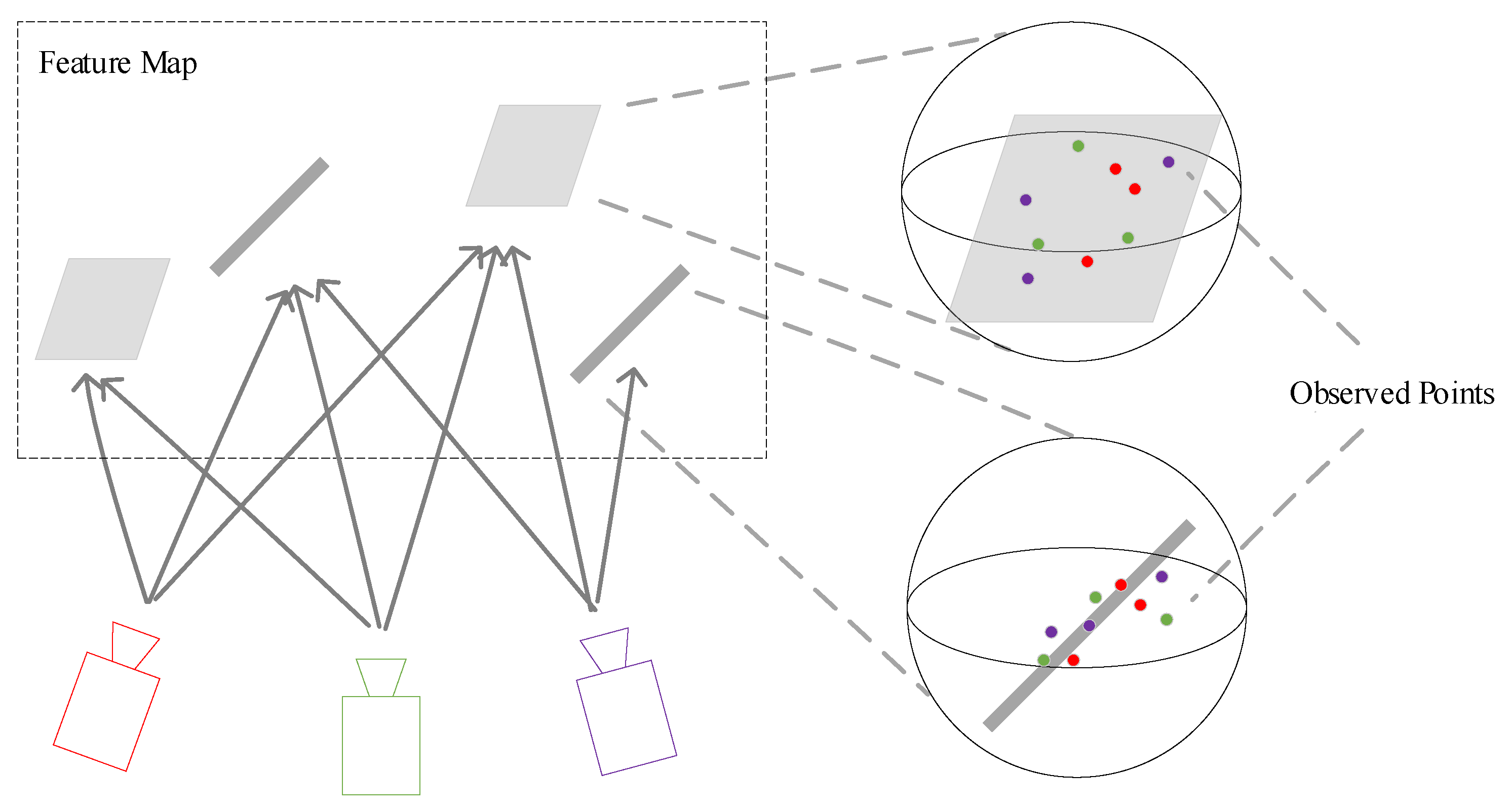
  • We present an efficient method for computing the covariance matrix of the feature points, which significantly reduces the computational complexity of bundle adjustment during the mapping stage.
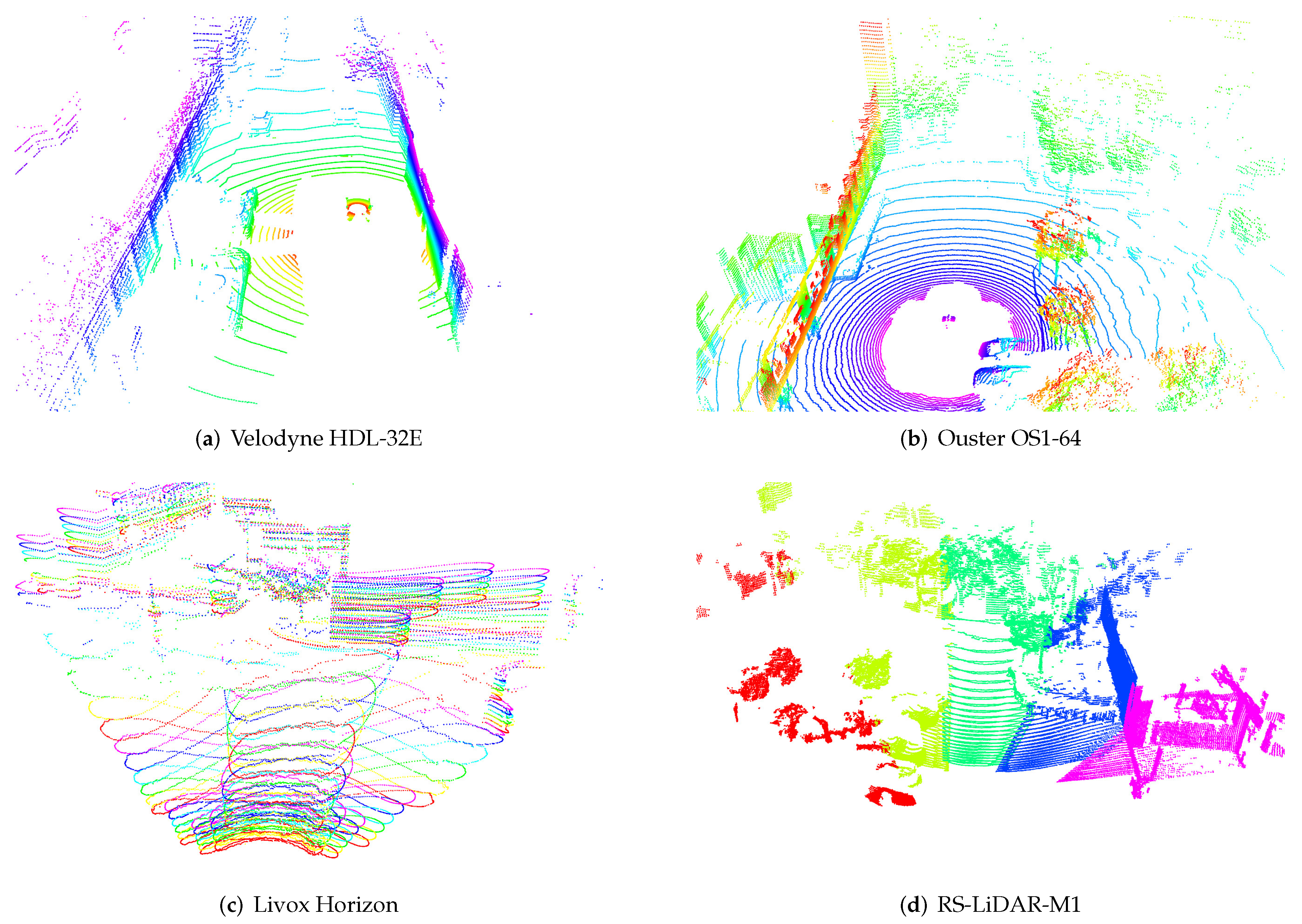
  • We test the performance of our algorithm on four types of LiDARs, including two rotor-based mechanical LiDARs and two solid-state LiDARs. The experimental results show that the proposed method can be applied successfully to these LiDARs and that it achieves higher precision than existing state-of-the-art SLAM methods.
The remainder of this paper is organized as follows. Section 2 describes the proposed method in detail, including the feature extraction, odometry, and mapping processes. Section 3 presents the experiments on the different datasets. Section 4 discusses the results. Finally, Section 5 presents the conclusions and directions for future work.

2. Method

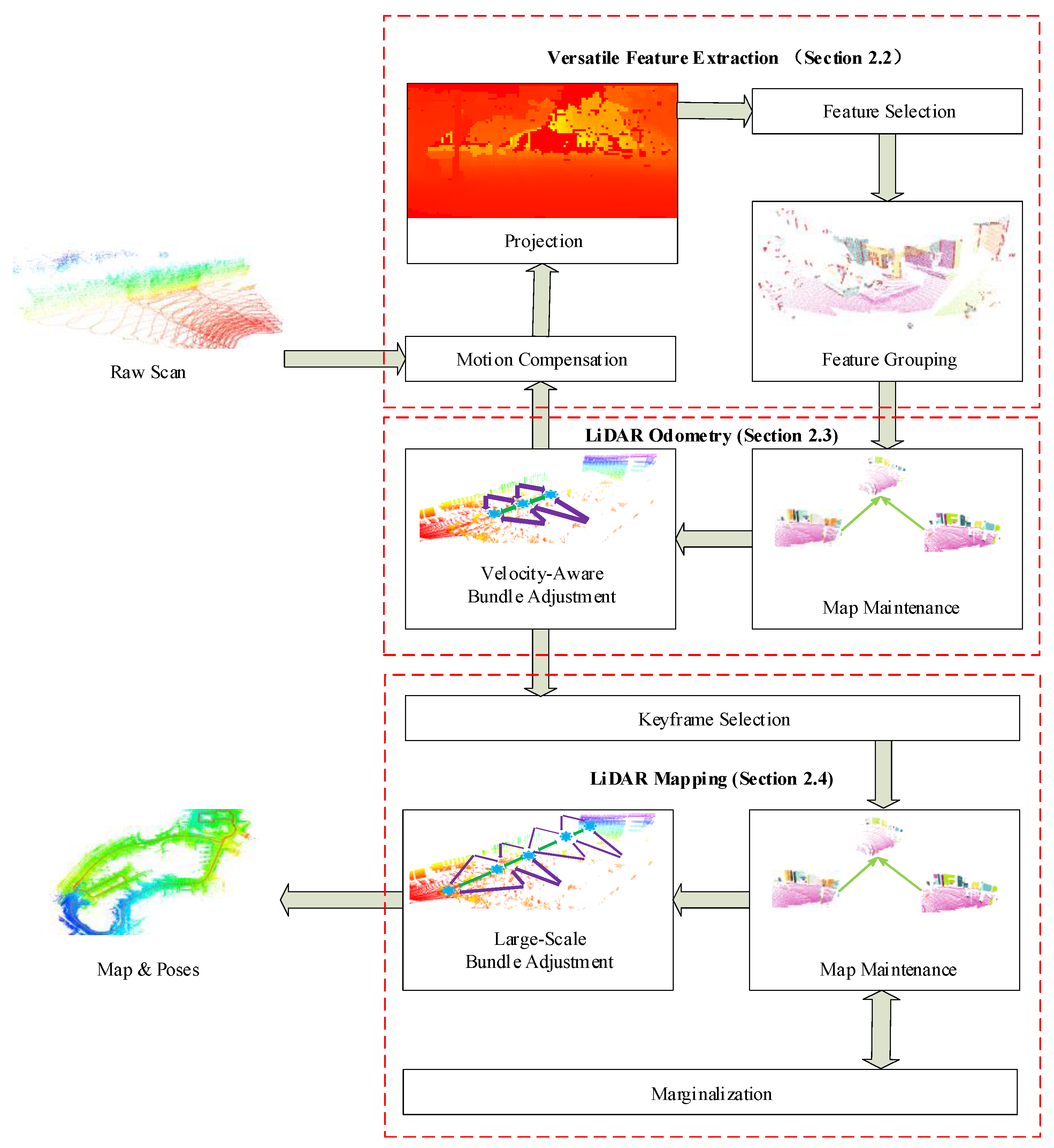
2.1. System Overview

Figure 2 depicts the workflow of the proposed SLAM system. The system processes raw point clouds from a 3D LiDAR and outputs scan poses and feature maps. The system includes three main components: a versatile feature extraction module, a LiDAR odometry module, and a LiDAR mapping module. The feature extraction module projects the point cloud onto a spherical image and extracts planar and edge features using a patch-based method. A graph-based approach [35] is used to group feature points into meaningful clusters to filter out smaller objects. Then, the remaining feature points are used in the LiDAR odometry module to build a feature map and estimate the pose and velocity. Finally, after the keyframe decision step, the feature point is undistorted based on the pose and velocity estimated during the odometry stage. These undistorted features and estimated poses are fed into the LiDAR mapping module, which uses bundle adjustment with a larger window to produce the final result. In addition, the odometry and mapping modules use the same logic for map maintenance, with only a few parameters differing. Moreover, we developed a novel design in which the feature extraction and odometry modules are implemented in the same thread and work iteratively; thus, we can use the odometry estimation results to improve the feature extraction accuracy. This is particularly useful for scenarios in which a car is traveling at a high speed. The details of each module are presented in the following sections.
In this work, the point cloud of the k-th scan is represented as P k . The world frame and local frame of P k are denoted as { W } and { L k } , respectively. For convenience, { W } coincides with { L 0 } . Since P k is acquired sequentially with the LiDAR motion, each point in P k is sampled at a different position, leading to ambiguity in the definition of { L k } . Therefore, it is important to note that we refer to the local frame { L k } as the frame defined by the first point in the k-th scan. Moreover, the transformation matrix from { L k } to { W } is denoted as T k Special Euclidean Group(3) ( S E ( 3 ) ):
T k = R k t k 0 T 1 ,
where R k Special Orthogonal Group(3) ( S O ( 3 ) ) is a rotation matrix and t k R 3 is a translation vector. The velocity, which has 6 degrees of freedom, is represented as V k = [ w k T , v k T ] T , where w k = [ w 1 , w 2 , w 3 ] T Lie algebra s o ( 3 ) and v k = [ v 1 , v 2 , v 3 ] T R 3 are the angular velocity and linear velocity, respectively. The angular and linear velocities are defined in the world frame { W } , which differs from most SLAM methods, as there is evidence that globally defined angular errors [36] have better properties. For simplicity, we assume that the angular and linear velocities are not coupled. Therefore, the transformation matrix T k j from any point j P k to { W } can be formulated as follows:
T k j = exp ( ( s k j s k ) w k ) R k ( s k j s k ) v k + t k 0 T 1 ,
where s k j is the timestamp of point j, s k is the start time of P k , which is equal to s k 0 , and exp ( w ) is the exponential mapping s o ( 3 ) S O ( 3 ) :
exp ( w ) = I + sin ( w ) w [ w ] × + 1 cos ( w ) w 2 [ w ] × 2 ,
where [ w ] × is the skew matrix of w . In addition, we define log ( · ) as the inverse map. For simplicity and clarity, we define a new function g that maps point j to its transformation matrix T k j shown in Equation (2):
g ( T k , ( s k j s k ) V k ) = T k j .

2.2. Versatile Feature Extraction

One of our most important contributions is the proposal of a versatile and efficient feature extraction algorithm based on spherical projection. Spherical projection is a widely used method in the community [21,23,37]. The spherical image is capable of representing point clouds from various LiDAR devices. As far as we know, this is the first attempt to extract planar and edge points based on spherical projection for LiDAR-based SLAM. A detailed analysis of each point based on the point-to-plane or point-to-line metric is performed on the spherical image to find more accurate feature points. Then, we use a customized connected component labeling [35] technique to group the point cloud and filter out more outliers. Finally, the selected planar and edge features are passed to the odometry and mapping module to obtain an estimate of the pose of the current scan.
Conventional methods distinguish feature points using a smoothness metric [16]. The metric simply compares the distance between a point and its surrounding points, which cannot describe a plane or edge well and easily leads to misclassification. To improve the quality of the extracted features, we develop a new method based on the spherical image, in which the feature point is selected based on accurate point-to-line and point-to-plane distances.

2.2.1. Motion Prediction and Point Cloud Compensation

Current methods typically use raw point clouds for feature extraction, which implicitly assumes that all points in a scan are acquired in the static state. However, the ego motion of LiDAR violates this assumption; thus, a reduced feature extraction performance is expected. In contrast, we use a coarsely undistorted point cloud for feature extraction, allowing us to better distinguish different features. After the odometry process is completed for the current scan, as discussed in Section 2.3, the accurate motion compensation procedure is repeated. Therefore, our algorithm performs the distortion compensation process twice.
Let s k be the start time of a new scan. The initial estimations of the transformation matrix T ^ k and velocity V ^ k can be predicted immediately from the previous scan with the constant motion model:
T ^ k = g ( T k 1 , ( s k s k 1 ) V k 1 ) V ^ k = V k 1 , k 2
where T k 1 and V k 1 are the transformation matrix and velocity obtained from the previous scan (see Section 2.3) and s k 1 is the timestamp of the previous scan. For the first scan, T ^ 1 is set to the identify matrix, and V ^ 1 is set to zero. For a point j in the current point cloud P k , let s k j be its timestamp; then, its transformation matrix T ^ k j can be obtained using Equation (2). Then, the transformation matrix that projects point j into the local frame of P k is T ^ P k j = T ^ k 1 T ^ k j . Assuming that p k j is the position of point j, the new position p ˜ k j after compensation can be calculated as follows:
p ˜ k j = R ^ P k j p k j + t ^ P k j ,
where R ^ P k j and t ^ P k j are the rotation and translation components of T ^ P k j , respectively.

2.2.2. Classification of Planar Features

The planar features are classified in three steps: spherical projection, planar point selection, and planar point grouping. In the spherical projection step, a spherical image is generated based on the coarse undistorted point cloud. In the planar point selection stage, a smoothness value is assigned to each point based on a fixed window and used to select planar points. In the planar point grouping stage, connected component labeling is employed to divide the point cloud into different planar groups. The use of an explicit point group allows us to filter out unreliable smaller objects, thus preventing false matches during feature tracking. Each step is explained in detail below.
Spherical Projection: For a point cloud P k after compensation, the corresponding spherical projection coordinate [ u , v ] T for a point p = [ x , y , z ] T P can be calculated as follows:
u v = M ( 1 arctan y x + f l e f t f r i g h t + f l e f t ) N ( 1 arcsin z r + f d o w n f u p + f d o w n ) ,
where r = x 2 + y 2 + z 2 is the distance of the point to the origin; [ f l e f t , f r i g h t ] , [ f d o w n , f u p ] are the vertical and horizontal fields of view of the LiDAR in terms of the radius, respectively; and M and N are the width and height of the projected image, respectively. M and N should be selected according to the LiDAR resolution.
Planar Point Selection: A patch-based method is used to select the planar points. Each patch is a 5 × 5 square region in the image. We approximate the local plane of a patch π using a fast method that requires only the four vertices { p 11 , p 15 , p 51 , p 55 } :
c π = 1 4 ( p 11 + p 15 + p 51 + p 55 ) n π = ( p 11 p 55 ) × ( p 51 p 15 ) ( p 11 p 55 ) × ( p 51 p 15 ) 2 ,
where c π is a planar point in π and n π is the plane normal of π . For a point p π , the point-to-plane distance can be calculated as d p = n π T ( p c π ) 2 . The points with values of d p less than the threshold α 1 are output as π S . Finally, the smoothness τ π of patch π is the mean value of π S .
Each point j in the image is included in several patches. Let π * be the patch with the smallest smoothness value; then, the smoothness and point normal of j are given by τ π * and n π * , respectively. Finally, the points with smoothness values less than the threshold α 2 are selected as planar points. By choosing the least smooth patch to determine the planar points, we can prevent misclassifying points at the plane intersection.
Planar Point Grouping: We group the planar points using an adapted connected component labeling algorithm. Connected component labeling is a technique that assigns the same label to all connected points in an image. We consider two adjacent points p 1 and p 2 to be connected if they satisfy the following conditions:
p 1 p 2 < 0.5 n 1 T n 2 > 0.9 ,
where n 1 and n 2 are normal vector of p 1 and p 2 , respectively. Each connected component represents a plane region with points that all belong to the same object. As a result, we can filter out objects with few points, since smaller objects are most likely noise. The label of each point serves as its feature ID. Finally, the planar features are downsampled for later use. The feature ID is used for tracking and to determine the map features to prevent inaccurate data associations.

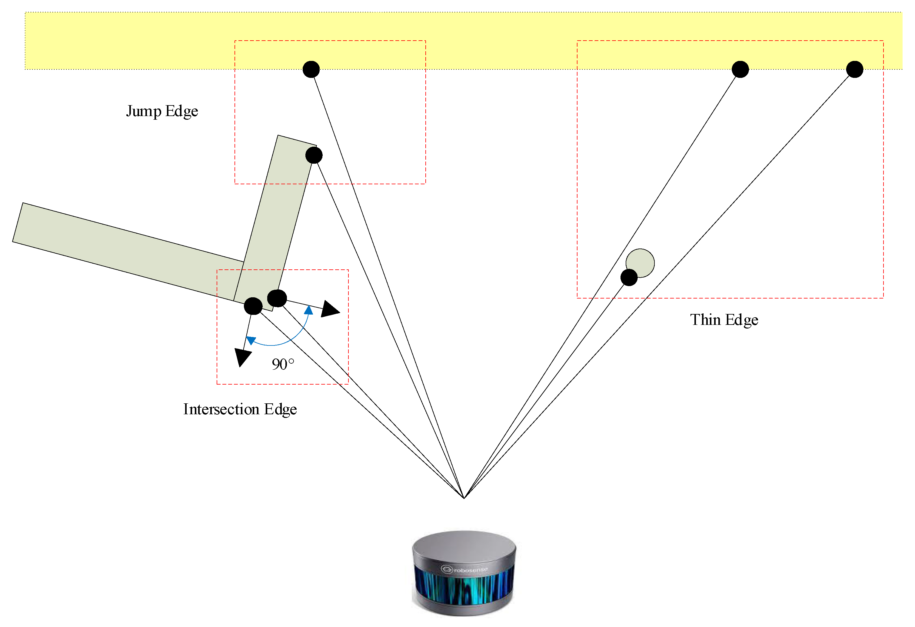
2.2.3. Classification of Edge Features

The edge features are detected based on the extracted planar features. We use the same selection-then-grouping scheme as in planar feature detection to extract the edge features.
Edge Point Selection: A two-step edge feature detection procedure is presented, in which the coarse edge features are first selected based on the extracted planar features and then used to identify more reliable edge features. Let p i and n i be the position and normal vector of a point i in an image. As shown in Figure 3, a point is selected as a coarse edge feature if any of the following three scenarios are applicable:
  • A point i is selected as an intersection edge feature if it and its neighboring point j are planar features with different planar feature IDs. Moreover, the position and normal of i and j must satisfy the conditions:
    p i 2 < p j 2 n i T n j < 0.5 .
  • A point i is selected as a jump edge feature if it is a planar feature with a significantly different depth than its neighboring point j:
    p j 2 p i 2 > 1 .
  • A point i is selected as a thin edge feature if its two adjacent points j and k in the same row or column satisfy the conditions:
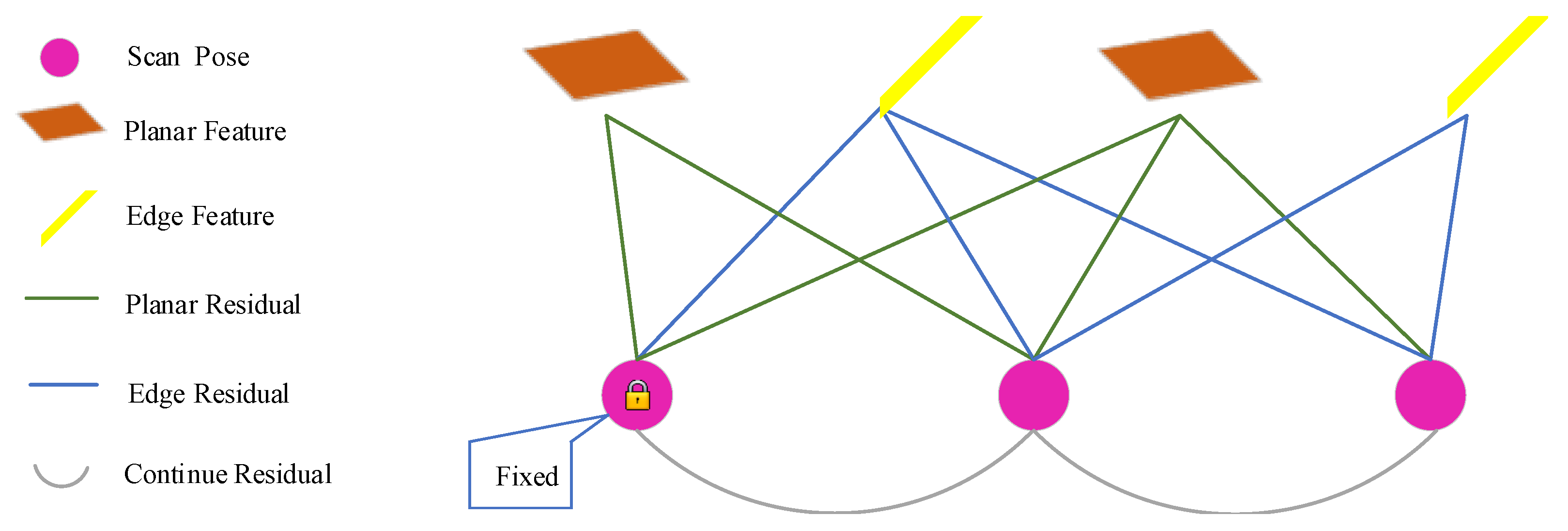
    p j 2 p i 2 > 1 p k 2 p i 2 > 1 .
Then, a new point cloud S is obtained by downsampling the coarse edge features. For each point p 1 S , we identify two neighboring points p 2 S and p 3 S using a KD tree. This tuple is represented as L. The direction vector n L and smoothness τ L of the tuple L are given as:
n L = p 3 p 2 p 3 p 2 2 , τ L = n L × ( p 1 p 2 ) 2 .
τ L also represents the distance from the center point p 1 to the line formed between its two neighboring points p 2 and p 3 .
Similar to the case in planar feature selection, a point in S can belong to several tuples. Let L * be the tuple with the smallest smoothness value. Then, the normal and smoothness of the point are given by n L * and τ L * . Finally, the points with smoothness values greater than the threshold β are filtered out. The remaining points in S are processed further and grouped.
Edge Grouping: Adapted connected component labeling is used to label the edge features. Two edge features are determined to be connected according to the above KD-tree search result and an additional metric, n 1 T n 2 > 0.8 , where n 1 and n 2 are the normals of the two edge points. Then, smaller clusters with less points are removed. The label of each point serves as its feature ID, which is used for tracking and identifying the map features.

2.3. LiDAR Odometry

The odometry module consists of two parts: Map Maintenance and Optimization. Map maintenance uses forward tracking as its core idea, which is inspired by π -LOAM [26]. We adapted this idea based on the proposed feature extraction method and developed a completely new feature tracking method. The developed method is more suitable for the pose optimization used in this work. The optimization is based on the bundle adjustment. The formulation for LiDAR bundle adjustment was first proposed by BALM [27]. However, BALM does not provide compensation for motion distortion, which may reduce the accuracy. Motion distortion is caused by the ego motion of the LiDAR, which results in each point in the point cloud being sampled at a different location. Based on the constant motion model, a unique pose can be assigned to each point to compensate for the distortion. Our main contribution is to jointly optimize the parameters of the constant motion model and the pose. The constant motion model ensures that our model better matches the real point cloud acquisition process, which can positively affect the accuracy of the estimation.

2.3.1. Map Maintenance

The map is a collection of map features, including planes and edges. A map feature is a spherical region fixed in 3D space that accumulates feature points from new scans that occur in its spherical region and satisfy certain conditions. Figure 4 shows an example of our map. We use a sliding window mechanism to ensure that the map size is bounded. After a new scan is inserted into the sliding window, the existing map features identify new feature points from the extracted features, and new map features are created from the remaining feature points. When the number of scans in the sliding window exceeds a certain size, three actions are performed to reduce the size of the map: (1) the oldest scan is removed, (2) the associated feature points are removed from the corresponding map feature, and (3) the map features with no feature points are removed. The detailed strategy for tracking and creating the global features is presented below:
Feature Tracking: The planar and edge features extracted from the current scan are denoted as H and E , respectively. We start by projecting map features that are neither edge nor planar features onto the current frame using the predicted transformation matrix from Section 2.2.1. Let c f be the center of a map feature f, and c ˜ f be the closest point to c f in the corresponding H or E . Then, we identify all feature points Q with the same feature ID as c ˜ f that belong to the spherical region of map feature f in the corresponding H or E . An eigenvalue decomposition of the covariance matrix of the 3D coordinates of Q is performed. Let λ 1 , λ 2 , λ 3 ( λ 1 λ 2 λ 3 ) be the eigenvalues of Q and n 1 , n 2 , n 3 be the corresponding eigenvectors. For a planar feature, we use the following conditions to determine whether Q should be added to f:
λ 1 λ 2 < 0.1 n 1 T n > 0.9 .
For an edge feature, we use the following conditions:
λ 2 λ 3 < 0.2 n 3 T n > 0.8 ,
where n is the normal vector or direction vector of the map feature f.
Feature Creation: New map features are created based on the remaining untracked features. For each untracked feature point j, we locate the K nearest neighbors in H or E , depending on the feature type. Then, we filter out points that have a feature ID different from j and denote the remaining points as D. We perform an eigenvalue decomposition on the covariance matrix of D. For the planar features, if the second largest eigenvalue is much larger than the smallest eigenvalue ( λ 1 λ 2 < 0.1 ), all points in D are extracted as new planar map features. For the edge features, if the largest eigenvalue is much larger than the second largest eigenvalue ( λ 2 λ 3 < 0.2 ), all points in D are extracted as new edge map features. Note that once a point is selected as a map feature, it is never selected again to ensure that there are no redundant map features. Finally, the center and radius of the map feature are calculated using D, and the normal vector or direction vector is saved.

2.3.2. Bundle Adjustment with Direct Velocity Estimation

The k-th scan in the current sliding window is denoted as F k . The full state vector X to be optimized in the sliding window can be expressed as follows:
X = { x 1 , x 2 , , x K } , x k = { R k , t k , w k , v k } ,
where K is the width of the current sliding window, and x k is the state of F k , where x k includes the rotation, position, angular velocity, and linear velocity of F k in the world frame.
Each map feature that is neither planar nor angular corresponds to a residual in the final optimization formula. Suppose f is a map feature, and p k j , j [ 1 , N k f ] are the tracked local points of f in F k , where N k f is the number of tracked points. N k f can be zero if there are no associated features in F k . To construct the residual of f, we must first project its observation points into the global coordinate system using the transformation matrix obtained with Equation (2). The projection can be performed using the following equation:
p ˜ k j = exp ( ( s k j s k ) w k ) R k p k j + ( s k j s k ) v k + t k ,
where p ˜ k j is the position of p k j in the world frame, s k is the start time of F k , and s k j is the timestamp of p k j . Equation (17) includes the velocity as a parameter, which is the main difference between our algorithm and BALM in the odometry stage. The velocity parameter, similar to the transformation matrix, is optimized during the final optimization process. The mean p ¯ and covariance A f of f can be calculated as follows:
p ¯ = 1 N f k = 1 K j = 1 N k f p ˜ k j A f = 1 N f k = 1 K j = 1 N k f ( p ˜ k j p ¯ ) ( p ˜ k j p ¯ ) T ,
where N f = k = 1 K N k f is the total number of feature points in f.
For a planar map feature f, the loss metric ε π f is the sum of the squared distances of all tracked points to the best-fitting plane, which can be calculated as:
ε π f = Λ 1 ( A f ) .
For the edge map feature, the loss metric ε L f is the sum of the squared distances of all tracked points to the best-fitting line, which can be calculated as:
ε L f = Λ 1 ( A f ) + Λ 2 ( A f ) .
Λ k ( · ) is a function that maps a matrix ( · ) to its k-th largest eigenvalue. The specific plane (or line) parameters are eliminated from ε π f (or ε L f ); the detailed procedure is the same as that of BALM [27]. Since the function Λ k ( · ) does not have a closed form, it is impossible to calculate the Jacobian matrix directly. Fortunately, BALM provides the first- and second-order Jacobians in closed form for the function Λ k ( · ) . Moreover, the results of ε π and ε L are quadratic, but we use the Ceres solver library [38] for optimization, which requires non-squared residuals. Therefore, we determine the final residual by directly computing the square root of ε π f and ε L f :
r π f ( X ) = ε π f = Λ 1 ( A f ) r L f ( X ) = ε L f = Λ 1 ( A f ) + Λ 2 ( A f ) .
Since we use a design with 12 degrees of freedom, it is difficult for the odometry module to guarantee perfect convergence, severely limiting the applications of the algorithm. This limitation can be addressed by introducing a continuous factor. This solution is very effective and allows our algorithm to produce valid results even in degenerate situations. The continuous factor is similar to the IMU pre-integration factor in VIO [39] and imposes a constraint on the motion of adjacent scans. The residual term of the continuous factor in the constant motion model can be defined as follows:
r s ( x k , x k + 1 ) = log ( exp ( ( s k + 1 s k ) w k ) R k R k + 1 1 ) ( s k + 1 s k ) v k + t k t k + 1 w k w k + 1 v k v k + 1 ,
We use M π and M L to represent the planar and edge map features in the current map, respectively. The final optimization problem can be expressed as a combination of Equations (21) and (22):
arg min X f M L ρ ( r L f ( X ) 2 ) + f M π ρ ( r π f ( X ) 2 ) + k = 1 K 1 r s ( x k , x k + 1 ) 2 .
where the Huber loss ρ is defined as follows:
ρ ( s ) = s s 1 2 s 1 s 1 .
We use the pose and velocity of the oldest scan in the current sliding window as a prior in the optimization process. The odometry factor graph is shown in Figure 5.

2.4. LiDAR Mapping

LiDAR mapping is based on odometry with some modifications to optimize the poses. Our process includes three enhancements: first, a keyframe selection step is added to reduce redundancy between scans. Second, the compensated point cloud is used as the mapping input; thus, the velocity does not need to be estimated. Third, a new formula for computing the covariance matrix is developed, which is faster than computing the covariance matrix directly from the raw points. The overall LiDAR mapping pipeline is similar to BALM [27] except for two improvements. One is the use of the feature map proposed in Section 2.3.1 and the other is the improved calculation method of the covariance matrix used in the optimization procedure.
The first step in the LiDAR mapping algorithm is to use a selection process to convert the new scans into keyframes, optimizing only the poses of the keyframes. To maximize sparsity while maintaining some degree of overlap between adjacent scans, the following criteria are used to determine if a new keyframe is needed:
  • The number of scans within the sliding window has not reached a preset value.
  • The ratio of the number of successfully tracked planar map features to the number of newly created features is less than 2.
  • The ratio of the number of successfully tracked edge map features to the number of newly created features is less than 1.5.
  • The time difference between the most recent frame and the last keyframe is greater than a specified value.
Each time a new keyframe is created, we use the odometry estimation result to remove distortions, as described in Section 2.2.1. Then, the undistorted features are added to the current map, and the pose of the new keyframe is optimized. The map maintenance and optimization processes are essentially identical to those in the odometry stage, and hence, we do not describe them here. Once the sliding window is full, a marginalization process based on the recursive form of the covariance matrix is performed [27,40], retaining the information of all points outside the sliding window using only a few parameters. Although the marginalization strategy is similar to those of most vision approaches, it is much simpler. The marginalization information is retained as a fixed component of the map feature and is added to the final covariance matrix. Moreover, the velocity can be eliminated from Equation (17), since we use an undistorted point cloud as the LiDAR mapping input. Therefore, Equation (17) can be simplified to:
p ˜ k j = R k p k j + t k .
The notations in the above formula are the same as those in Equation (17), except that p k j is the undistorted point. Then, we calculate the covariance of each map feature and form the residual using Equation (21). In addition, the removal of the velocity leads to the removal of the continuous factor from the optimization objective because the dimension of the optimization is reduced. Thus, the entire optimization objective can be reduced to:
arg min X f M L ρ ( r L f ( X ) 2 ) + f M π ρ ( r π f ( X ) 2 ) .
In the following section, we discuss a technique for accelerating the computation of the covariance matrix A f in residuals.

2.4.1. Fast Computing for A f

The computation of the LiDAR residuals r L f and r π f can be decomposed into two steps: the computation of the covariance matrix A f and the eigenvalue decomposition. The formal component must be computed from all feature points of a given map feature. We demonstrate a technique for computing A f by storing only a small matrix and vector for each scan and eliminating the dependencies of the raw feature points. Equation (18) can be rewritten as follows:
A f = 1 N f ( k = 1 K j = 1 N k f p ˜ k j p ˜ k j T C ˜ k 1 N f ( k = 1 K j = 1 N k f p ˜ k j S ˜ k ) ( k = 1 K j = 1 N k f p ^ k j S ˜ k ) T ) = 1 N f ( k = 1 K C ˜ k 1 N f ( k = 1 K S ˜ k ) ( k = 1 K S ˜ k ) T ) ,
where the notations are the same as those in Equation (18). Suppose C k = j = 1 N k p k j p k j T , S k = j = 1 N k p k j . Equation (25) can be substituted into C ˜ and S ˜ ; after the equation is simplified, we obtain:
C ˜ k = R k C k R k T + R k S k t k T + t k S k T R k T + N k f t k t k T S ˜ k = R k S k + N k f t k .
Since C k and S k are irrelevant to the pose of the current frame, C k and S k can be calculated in advance. With Equations (27) and (28), we can perform a fast computations of A f and reduce the large number of calculations required during the optimization process. Since the number of scans is often small, this method for computing A f can significantly reduce the memory requirements and computational complexity.

3. Experimental Results

We implemented the proposed algorithms in C++ and ran them using a robot operating system (ROS) [41] on a desktop with an Intel i7-9700 CPU and 16.0 GB of RAM. To the best of our knowledge, this is the first time that spherical projection has been used to unify inputs from different LiDARs. We achieved results comparable to other state-of-the-art approaches by simply adjusting some parameters for each type of LiDAR. Four types of LiDARs were used in our evaluation: Velodyne HDL-32E, Ouster OS1-64, Livox Horizon, and RS-LiDAR-M1. The detailed results are explained below.

3.1. Evaluation Metrics

Two metrics were used to evaluate the results of the different algorithms. The first was the relative pose error (RPE), and the second was the end-to-end position error. The RPE corresponds to the local drift in the trajectory. The EVO library [42] was used to compute the RPE. All estimated trajectories were aligned with the ground truth using S i m ( 3 ) Umeyama alignment over the EVO library. We assume that T k and T k + δ are the estimated poses of the ground truth G k and its successor G k + δ , respectively; then, the RPE at time k can be defined as:
R P E k = ( G k 1 G k + δ ) 1 ( T k 1 T k + δ ) ,
The RPE has two parts: the rotation component, which is known as the relative rotation error (RRE), and the translation component, which is known as the relative translation error (RTE). The mean and root mean square metrics were used to combine the results of the entire trajectory.
Moreover, the end-to-end position error was used for the Livox Horizon dataset, because no ground truth trajectory was available.

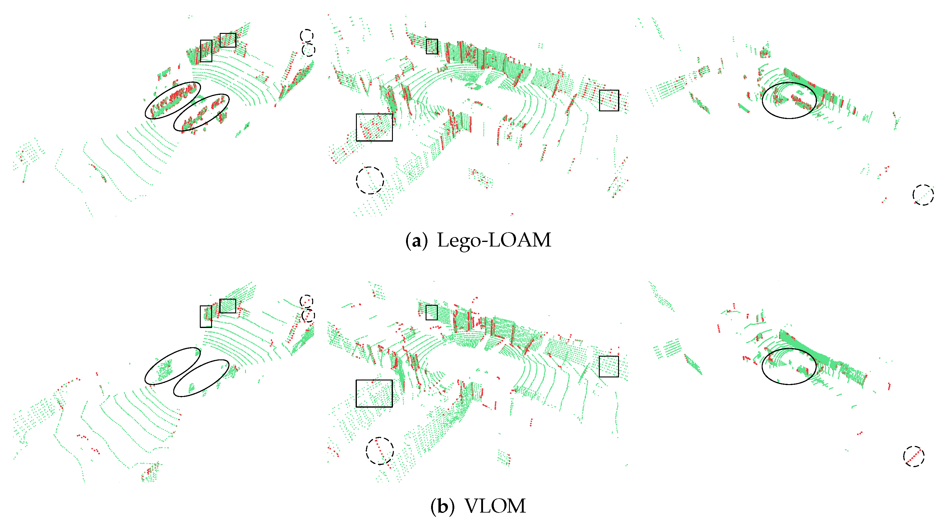
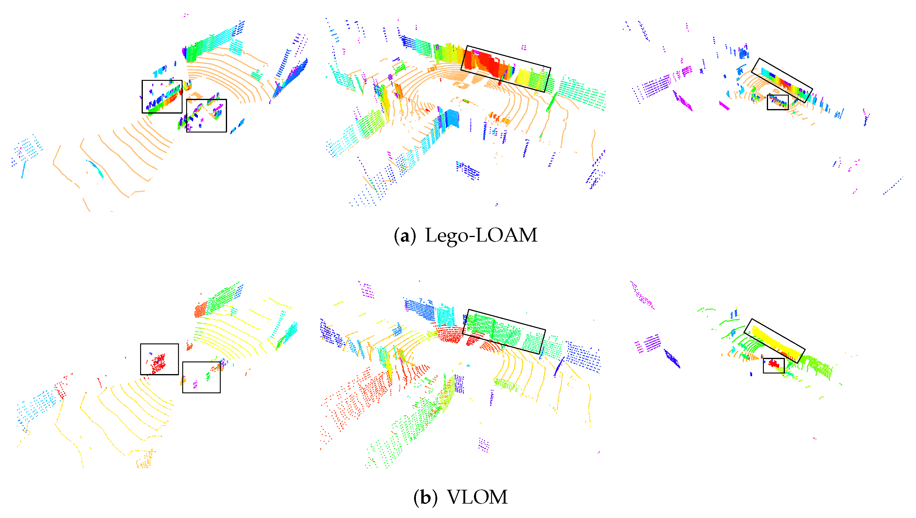
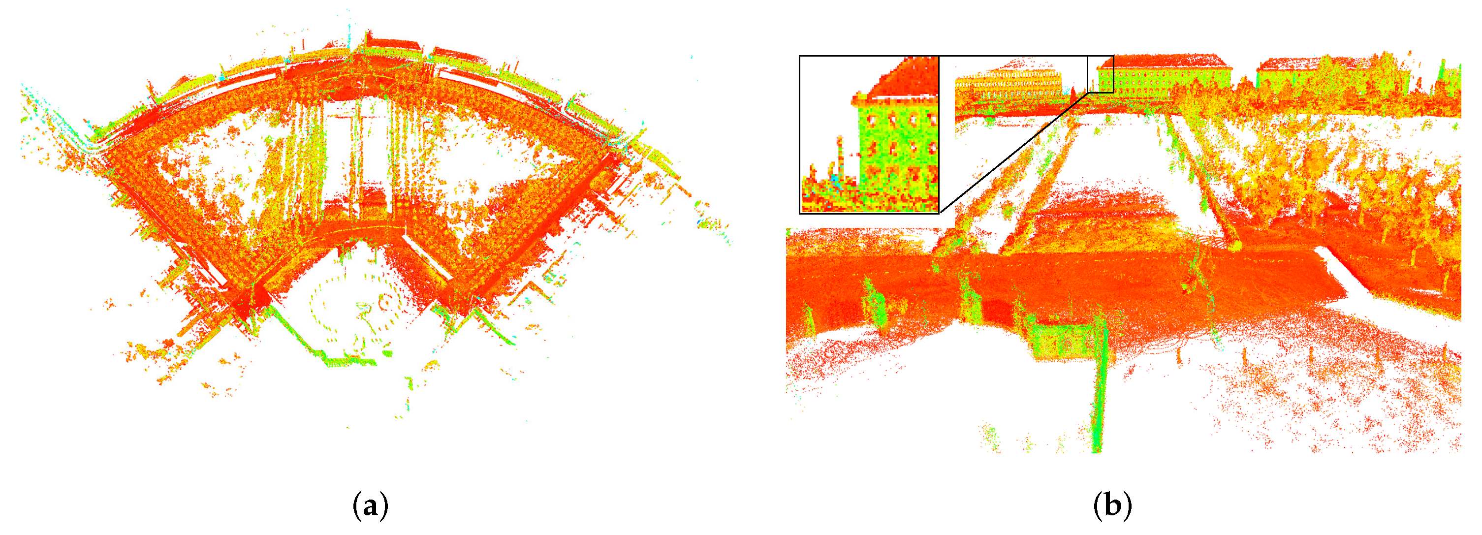
3.2. Feature Extraction Results

Feature extraction is an important component in the SLAM algorithm and has a considerable impact on subsequent pose estimation tasks. The Lego-LOAM method uses the segmentation information to extract features. We compare VLOM with Lego-LOAM using some representative scenes from the UrbanLoco dataset [43]. The results are shown in Figure 6. The planar and edge features are colored green and red, respectively.
VLOM detects more correct edge features than Lego-LOAM (the dashed circle in Figure 6). Lego-LOAM misclassifies these edge features as planar features. The feature selection module of Lego-LOAM depends on the smoothness of the scan line, which is not suitable for accurately classifying points. The correct identification of these edge features is crucial for stable tracking. Moreover, because VLOM uses accurate point-to-line and point-to-plane distances to determine the feature points, VLOM does not classify planar points as edge points (the rectangle with a solid line in Figure 6). In addition, Lego-LOAM classifies a large number of points from nearby dynamic cars as edge features (the ellipse with a solid line in Figure 6). However, such features are detrimental to the performance of the algorithm. In contrast, VLOM almost completely filters out these points.
Figure 7 shows the segmentation results for the same scenes. The various colors indicate different planes. Lego-LOAM does not segment planes; instead, it segments connected objects. Figure 7 shows that the ground and wall points are grouped correctly. Lego-LOAM is excellent at classifying ground points. Although VLOM divides the ground points into multiple clusters, this has no effect on our feature selection result because each cluster is large enough that it is not filtered out and can thus provide plane information. This good segmentation result is critical since it allows us to use points at the intersections of the planes as edge features. In addition, VLOM performs better near the wall than Lego-LOAM (the rectangle in Figure 7). The excellent feature classification performance of VLOM results in stable tracking. The segmentation results may also provide additional information for subsequent identification and obstacle avoidance tasks.

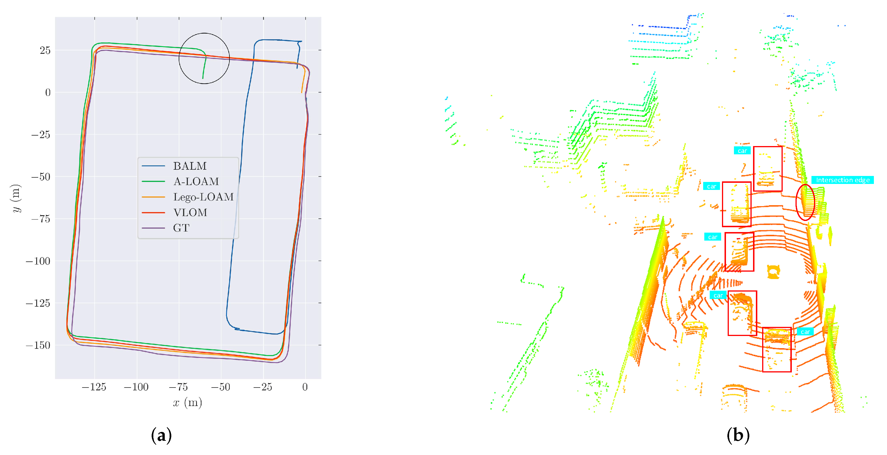
3.3. Evaluation on Velodyne HDL-32E

The sequence, namely HK-Data20190117, in this section was taken from the UrbanLoco dataset [43]. HK-Data20190117 were acquired with a Velodyne HDL-32E laser scanner at a rate of 10 Hz . The ground truth was acquired with Novatel SPAN-CPT, which is an integrated GNSS/INS navigation system with a position error of less than 2 cm . Since GNSS signals are easily affected by occultation and weather conditions, the selected sequence was acquired in a light urban area with good satellite visibility (as indicated by the author). HK-Data20190117 is a challenging dataset for LiDAR-based SLAM tasks because it includes a large number of dynamic objects, which can result in incorrect data associations and lower localization accuracy. In addition, the sequence provides a ground-truth linear velocity, which we used to evaluate our direct velocity estimation method.
For comparison, the most advanced pipelines were selected, including BALM, A-LOAM [44], and Lego-LOAM; the results are shown in Table 1. A-LOAM is an open-source implementation of the original LOAM algorithm. BALM replaces the mapping module of LOAM with a bundle adjustment approach. Based on Table 1, we can conclude that our method achieves higher accuracy than the other methods.
Figure 8a shows the estimated trajectories of each method versus the ground truth. As seen in Figure 8a, VLOM agrees with the ground truth across the entire trajectory and achieves a higher accuracy than the other methods. BALM and A-LOAM have significant tracking losses at various positions. Figure 8b shows a representative scene in which A-LOAM was unable to complete the tracking. This scene included many vehicles (indicated by the rectangle in Figure 8b) that were traveling parallel to the data collection vehicle. As a result, the A-LOAM algorithm could not detect any movement, and the trajectory was stationary for some time. Although Lego-LOAM performed better on this scene than A-LOAM, Lego-LOAM was also affected to some extent, with a significant error in the end position. BALM uses a voxel grid to capture feature associations; this method results in a lower accuracy and thus may not be flexible enough for complex real-world scenarios. As a result of our precise feature extraction method, VLOM is less affected by dynamic objects and can achieve a stable tracking performance.
To investigate the effectiveness of our feature selection scheme, we replace the feature extraction module of BALM and A-LOAM with our method. Since Lego-LOAM must clearly distinguish between ground features and non-ground features, it is not compatible with our method and therefore is excluded from this evaluation. The updated algorithms with our feature module are denoted as BALM-F and A-LOAM-F. Figure 9 shows a comparison of the new algorithms. The considerable tracking loss of the original methods disappeared, and consistent trajectories were obtained. Moreover, the RMSEs of the RTEs reached 0.286 and 0.267 for BALM-F and A-LOAM-F, respectively. This result proves that our feature extraction module is more accurate and robust than the other methods.

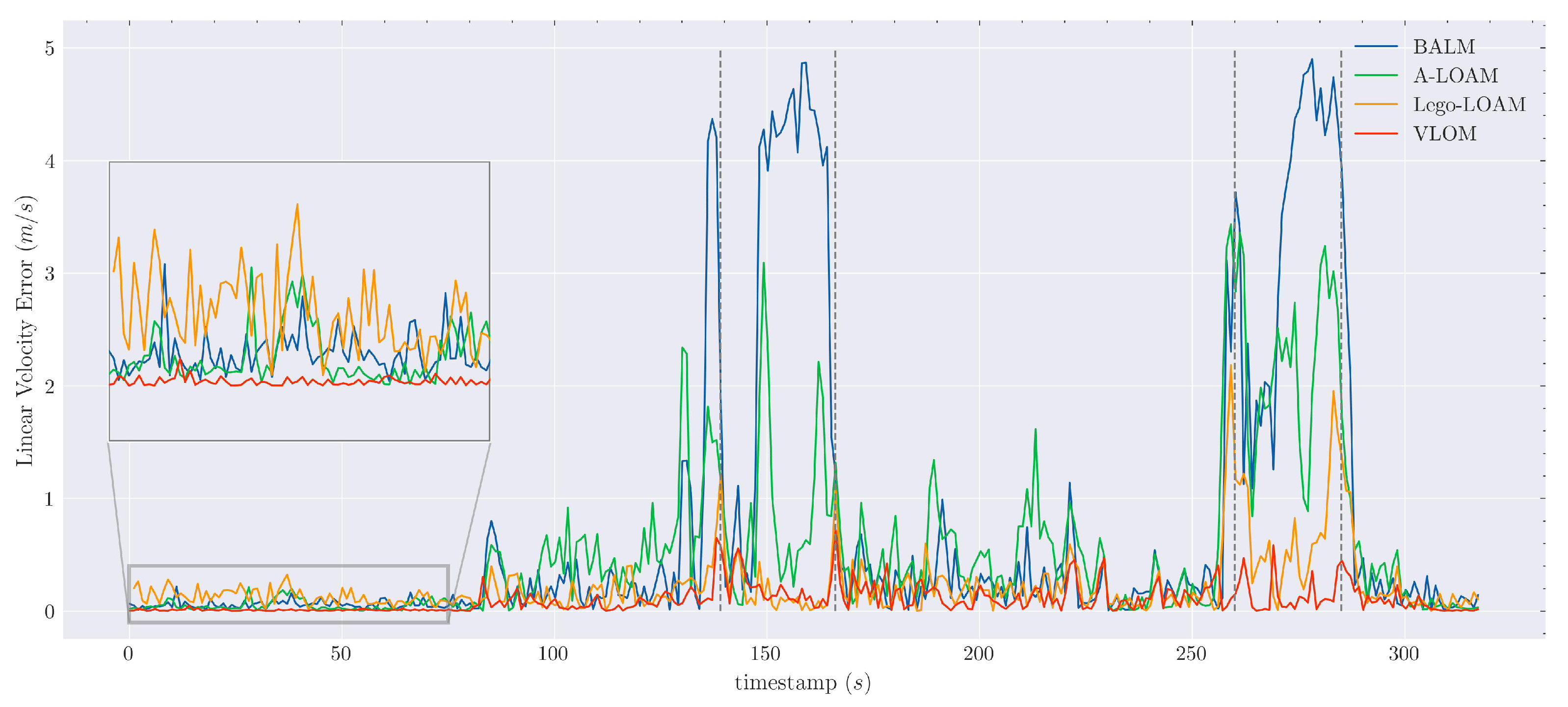
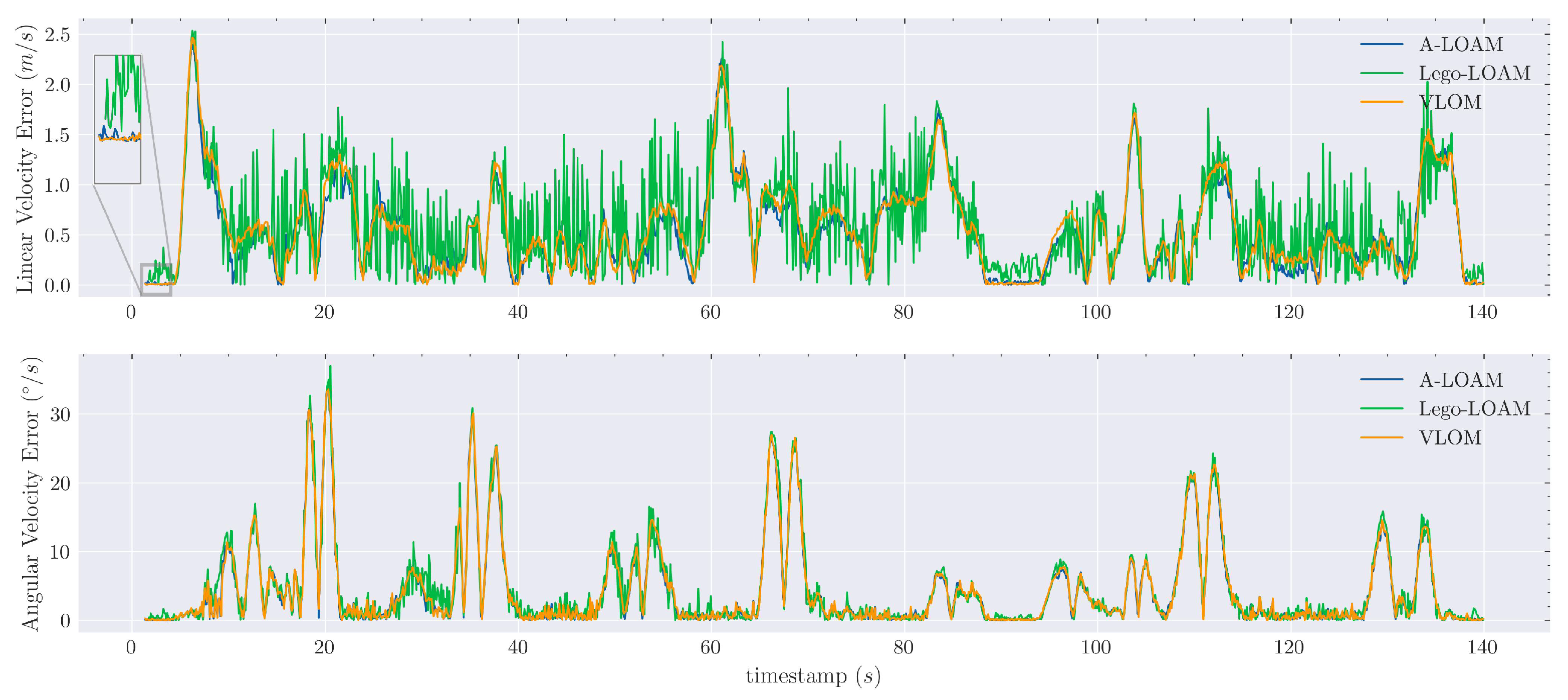
3.3.1. Evaluation of the Velocity Estimate

The most important function of the odometer is the velocity estimation [45]. An accurate velocity estimation is crucial for recovering a time-aligned point cloud that has been distorted by the ego motion of the LiDAR. Let T ˜ k and s k be the odometry output and timestamp of the k-th scan, and let the linear velocity v k G T and angular velocity w k G T be the corresponding ground truth. For the BALM, A-LOAM, and Lego-LOAM methods, the velocity can be determined according to the relative transformation of the neighboring scans. For these methods, we define the following error metrics:
e k v = 1 s k + 1 s k Trans ( T ˜ k 1 T ˜ k + 1 ) 2 v k G T 2 e k w = 1 s k + 1 s k log ( Rot ( T ˜ k 1 T ˜ k + 1 ) ) 2 w k G T 2 ,
where Trans ( · ) and Rot ( · ) are the translation and rotation components of ( · ) , respectively, and e k v and e k w are the errors of the linear and angular velocities of the k-th scan, respectively. Since the velocity is calculated explicitly in VLOM, the error can be expressed as follows:
e k v = v ˜ k 2 v k G T 2 e k w = w ˜ k 2 w k G T 2 ,
where v ˜ k and w ˜ k are the odometry velocity output of VLOM. The above definitions of e k w and e k v are based on the L2 norm, which eliminates the difficult task of aligning the estimated trajectory with the ground truth.
Since the UrbanLoco dataset does not include the angular velocity, we evaluated only the linear velocity. The results are shown in Figure 10. As seen from the magnified area in Figure 10, the car remained in the start position for an extended period of time. Lego-LOAM had a low stability and a large error at this stage. However, while driving, BALM and A-LOAM performed worse than Lego-LOAM. Although Lego-LOAM showed excellent accuracy, the region marked by the vertical dashed line in Figure 10 shows that Lego-LOAM had substantial errors. These regions correspond to the four corners of the overall sequence, indicating that the iterative velocity estimation algorithm cannot handle rotation distortions. In contrast, VLOM performed well on the entire sequence. Thus, the combination of bundle adjustment with direct velocity estimation allows for a tremendous improvement in terms of velocity accuracy.

3.4. Evaluation on Livox Horizon

Livox Horizon is a solid-state LiDAR with a circular FoV of 81.7 ° (horizontal) × 25.1 ° (vertical) and a non-repeating scan pattern. Since solid-state LiDAR is a new technology, there are few publicly available datasets. We selected the KA-URBAN-Schloss-2 sequence (abbreviated as Schloss-2), which was provided in the work on LiLi-OM [34]. Schloss-2 was recorded at a typical sampling rate of 10 Hz while traveling with a sensor suite in Karlsruhe, Germany. The total length of this sequence is approximately 1.10 km . The walking speed is approximately 1.49 m / s . The author does not provide the ground-truth trajectory. Therefore, the RPE is not available. For quantitative comparison, because the sequence ends at its starting position, the end-to-end position error can be used as an evaluation metric.
A-LOAM and Lego-LOAM were developed for conventional LiDAR and thus are incompatible with Livox Horizon. Therefore, Livox-Horizon-LOAM (abbreviated LiHo) [46] and BALM were used for comparison. LiHo is an LOAM variant that was adapted to Livox Horizon with a specially designed feature extraction module. In this study, we supported LiHo with IMU. The result is shown in Table 2, and the entry after “/” shows the result with IMU. In addition, we directly report the LiLi-OM result from their article. LiLi-OM is a state-of-the-art tightly coupled LiDAR inertial odometry. VLOM significantly outperforms the LiDAR-only systems. It is worth noting that after extensive testing, we found that this sequence has several frame losses (with a maximum time interval of 0.43 s ), which negatively impacts our system because relatively long time intervals violate the constant motion assumption. This shows that our system is highly robust. Moreover, the results show that VLOM outperforms LiLi-OM, which has a special configuration for Schloss-2. This indicates some similarity in the roles of the direct velocity estimation and IMU, prompting us to reconsider the value of in-scan motion for LiDARs.
Figure 11a shows a top view of the final map of Schloss-2 produced by our method, and Figure 11b shows a side view of a representative structure place. The color is based on the intensity value. The map preserves fine structural details of the environment due to our accurate estimation of the scan velocity.

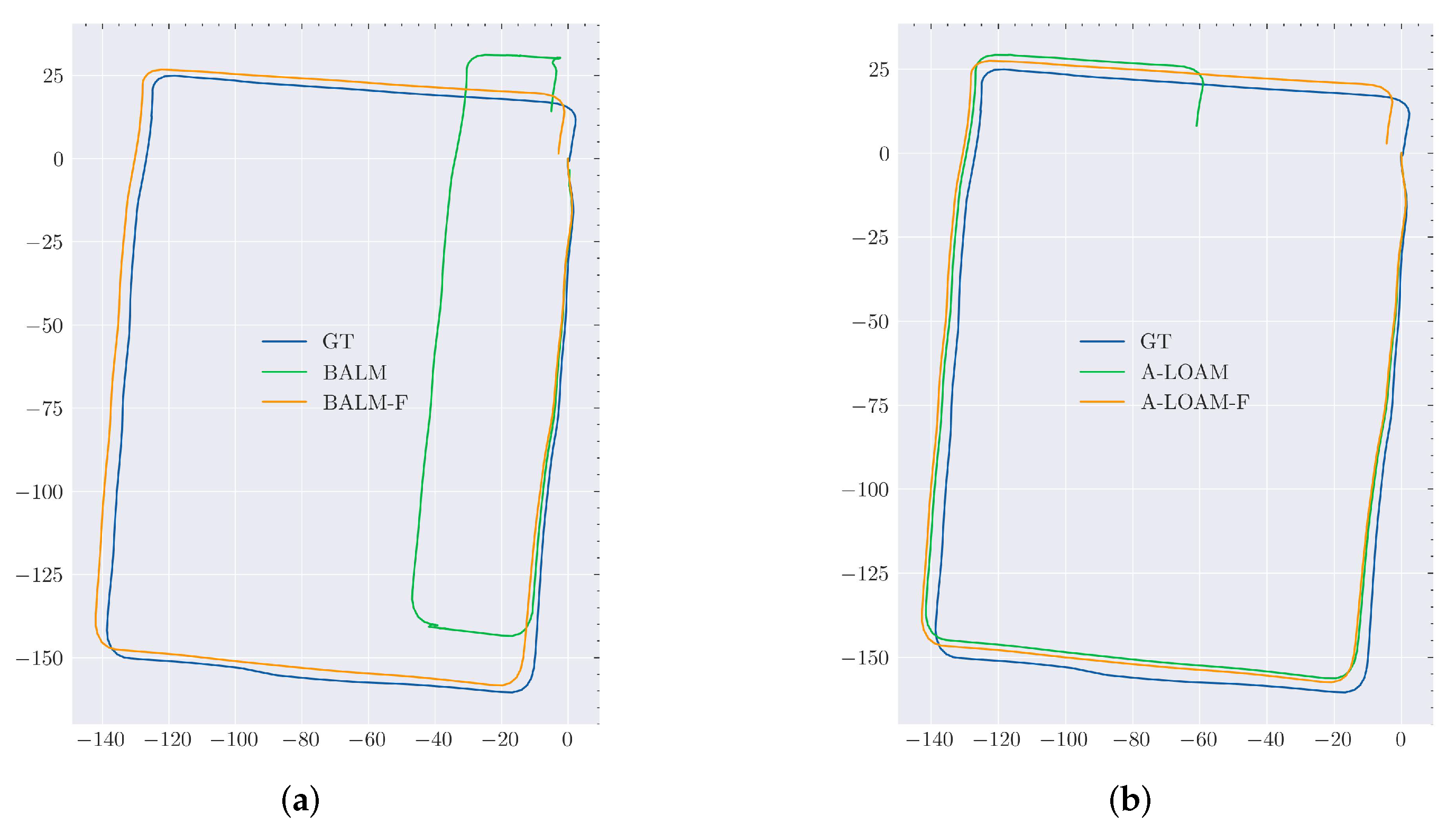
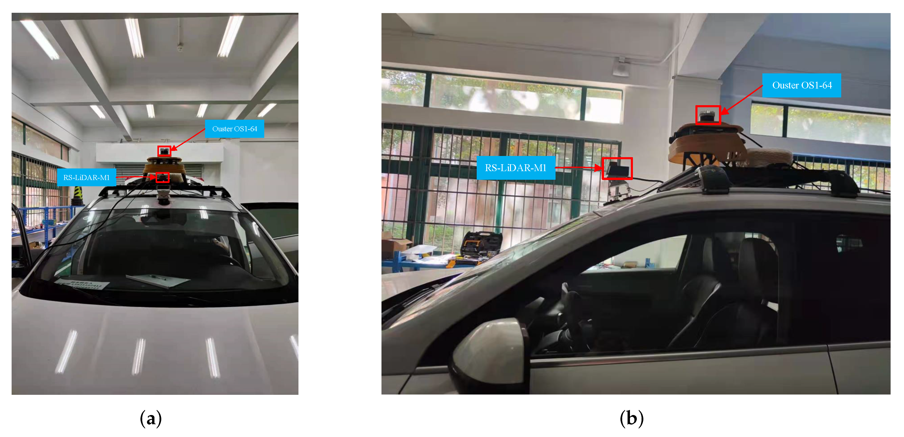
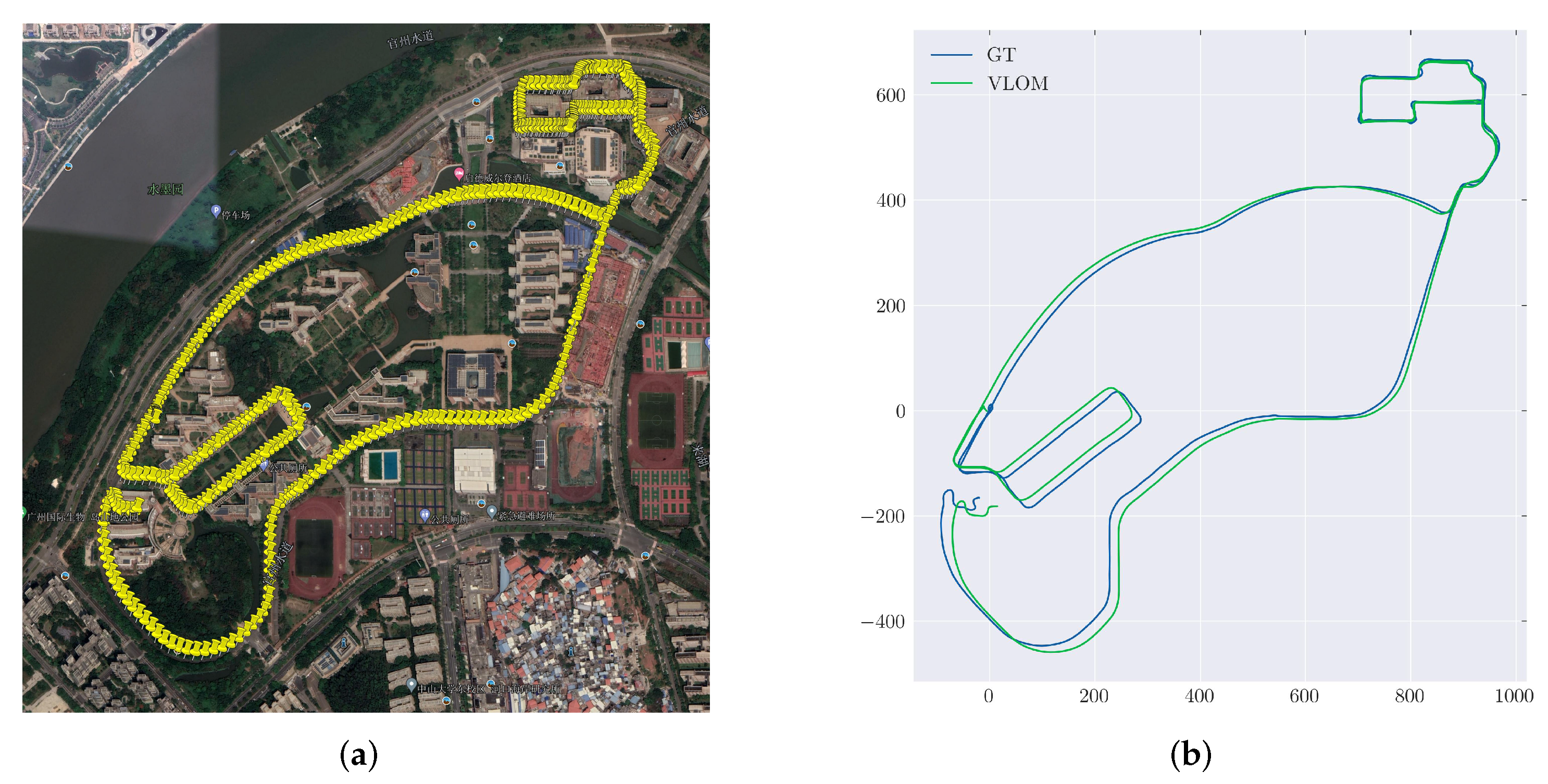
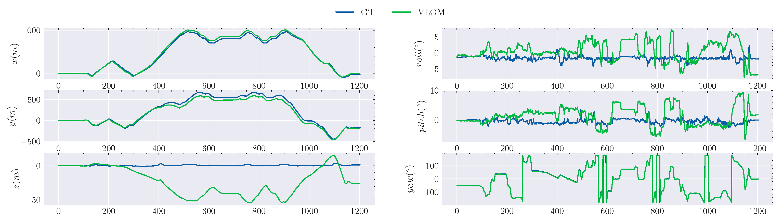
3.5. Evaluation on Our Campus Dataset

To test the performance of VLOM on real-world scenarios, we built a sensor suite using a conventional LiDAR, Ouster OS1-64, and a newly released solid-state LiDAR, RS-LiDAR-M1. RS-LiDAR-M1 has a resolution of 0.2 ° in the horizontal and vertical directions and an FoV of 120 ° (horizontal) × 25 ° (vertical). The datasets were acquired at a frequency of 10 Hz using an RS-LiDAR-M1 sensor installed horizontally on the front of a vehicle and an Ouster OS1-64 sensor installed horizontally on the roof. We used an integrated high-end Newton-M2 navigation device to obtain the ground truth. Newton-M2, when used in conjunction with a differential GNSS, can achieve a position accuracy of 2 cm and an attitude error of approximately 0.1 ° . The complete experimental platform is shown in Figure 12. Two sequences were collected by manually driving a car through the eastern campus of Sun Yat-sen University. The sequence corresponding to RS-LiDAR-M1 has a length of 5.94 km and is denoted as RS. The sequence corresponding to Ouster OS1-64 has a length of 1.37 km and is denoted as OS. The average velocity of both sequences is approximately 6 m / s .
The comparison results of BALM, A-LOAM, Lego-LOAM, and VLOM on OS are shown in Table 3. Since A-LOAM does not support Ouster OS1-64, we performed some minor changes. The results show that BALM has large translation errors and that our method performs better than the other methods. Since the OS dataset was collected on a narrow street surrounded by buildings, there are no large terrains in the dataset, resulting in a larger error with Lego-LOAM.
Since previous works have not included RS-LiDAR-M1, only VLOM was assessed on the RS dataset. The ground truth aligned to Google Earth is shown in Figure 13a, and the estimated trajectory of VLOM is shown in Figure 13b. Since there is no module that can close the loop, drift is inevitable, yet our results rarely overlap with the ground truth. Moreover, Figure 14 shows the deviations in the position and orientation. The error is mainly caused by [ z , r o l l , p i t c h ] , implying that the constraints in the vertical direction are insufficient. Since these constraints are mainly imposed by the ground features and the main direction of the LiDAR sensor is parallel to the ground, it is difficult to effectively extract features.

Evaluation of the Velocity Estimate

The velocities are compared in Figure 15. Since BALM has large errors on the OS dataset, the corresponding data are not shown here for clarity. A-LOAM and VLOM have overlapping curves and show similar performance; however, the magnified area at the top of Figure 15 shows that VLOM performs slightly better than these methods. Lego-LOAM appears to be unstable on the OS dataset and has more jitters.

3.6. Evaluation of Runtime

Furthermore, we calculate the average runtime of each module for all sequences used in the experiments; the results are shown in Table 4. Since the feature extraction and LiDAR odometry modules in VLOM operate in the same thread, we consider the total time spent by both and report it as Feature + Odometry. To evaluate the effect of the fast covariance calculation method proposed in Section 2.4.1, we carried out an experiment with the same conditions as Equations (27) and (28) and report the results as Old and New, respectively. VLOM demonstrates real-time performance capability (less than 100 ms at the LiDAR frame rate). By comparing the Old and New results, we can conclude that the new method effectively reduces the runtime.

4. Discussion

Feature extraction: Feature extraction is an important component of many LiDAR-based SLAM algorithms. The feature extraction module often determines whether the algorithm can be used with a particular LiDAR type. The experiments in Section 3 show that only VLOM can complete all sequences (the other methods are incompatible with RS). In addition, the BALM algorithm supports both conventional LiDARs and solid-state LiDARs (Livox Horizon). However, BALM uses different feature extraction modules for conventional LiDARs and solid-state LiDARs. Depending on the LiDAR used, different startup programs need to be executed. Without adaptation, there may be the new LiDAR type to which BALM cannot be applied (e.g., RS -LiDAR-M1). The adaptability of VLOM is improved by our spherical projection-based feature extraction module. In addition, the spherical projections allow us to perform more detailed analyses of the planes and edges, improving the quality of the extracted features. This improvement was confirmed by the experiments with A-LOAM-F and BALM-F shown in Figure 9. Both algorithms with good results were developed by replacing the feature extraction modules of the original A-LOAM and BALM algorithms.
Velocity estimation: As described in Section 3.3.1, the velocity can be estimated either directly or based on the poses of two frames, followed by interpolation. Most open-source algorithms are based on the latter scheme. However, this can lead to closed loops between the pose and velocity estimates: the pose estimate requires that the velocity estimate produces an accurate and undistorted point cloud, while the velocity estimate, in turn, relies on the pose estimate. This type of iterative process cannot be repeated infinitely. In fact, most algorithms perform very few iterations; thus, it is difficult to achieve an accurate result in complex scenarios. This trend can be observed in Figure 10 and Figure 15. Since the HK-Data20190117 sequences were collected on a street surrounded by a complex environment, the velocity accuracies achieved by A-LOAM, BALM, and Lego-LOAM were lower than that achieved by VLOM; however, because the OS dataset was collected on a campus surrounded by several buildings and few people, A-LOAM and VLOM had similar velocity accuracies.
We assume that the LiDAR is moving at a constant speed. However, since SLAM is a probability estimation problem, some error is acceptable, so this algorithm can work in most real scenarios with non-constant velocity. In the experiments of this paper, a walking sequence (Schloss-2), two driving sequences on campus (OS and RS), and a driving sequence on a city street (HK-Data20190117) were studied. In particular, the walking sequence, which has a high degree of randomness, is very challenging. The good performance on these sequences proves that the algorithm in this work can handle the real-world scenarios with non-constant motion well.
Bundle adjustment: We use the scheme proposed by BALM for bundle adjustment. Bundle adjustment is a strategy that was first used in vision-based SLAM. In bundle adjustment, the previous frames and current frame are optimized together, achieving consistency over a wider range. However, when used with LiDARs, two problems arose: first, a single point could not be used to represent a complete landmark (i.e., planes and edges); thus, multiple points were required to determine a landmark in each frame. However, it is not easy to determine the appropriate sets of points. Second, the distortion of the point cloud caused by LiDAR motion led to inaccurate landmark observations. To address the first problem, BALM uses an adaptive octree to determine the observed point set and considers all points belonging to the same voxel as observations of the same landmark. False associations are generated for voxels located at the intersection of two landmarks. To address the second problem, BALM uses a LOAM variant in its front end to estimate the velocity and compensate for the point cloud. However, in our tests, the LOAM variant used by BALM showed poor real-time performance, which significantly reduced the speed of the algorithm. Thus, these solutions are inadequate. The results on the HK-Data20190117, Schloss-2, and OS sequences show that the bundle adjustment module of BALM is not robust enough, resulting in large deviations in these sequences. We address the first problem by using the strategy described in Section 2.3.1 to adaptively capture the set of observations of a landmark. By incorporating the intraframe velocity estimate into the optimization process, we can evaluate the motion compensation of the point cloud during the bundle adjustment process, which addresses the second problem quite well. VLOM significantly outperformed BALM on all sequences except the RS sequence, which is not supported by BALM.

5. Conclusions

In this work, we developed a SLAM system with 12 degrees of freedom that allows for real-time state estimation. Since the feature extraction module is designed for versatility, VLOM is suitable for both spinning and solid-state LiDARs. In addition, by directly estimating the velocity, we can produce a more accurate point cloud, improving the accuracy of LiDAR mapping. We also improved the efficiency of computing the covariance matrix, increasing the speed of bundle adjustment during the LiDAR mapping. With extensive tests on various LiDARs, we show that our algorithm performs better performance than various state-of-the-art methods.
We use spherical projection to unify all inputs, primarily because the spherical image is small and provides a fast method for finding nearest neighbors, which is important for real-time performance. However, there are many other representation options, such as bird’s eye view. In the future, other suitable representations can be explored to improve the performance of the feature extraction module. In addition, the proposed algorithm does not include a loop closure module, which is useful for reducing drift and is already used in many SLAM algorithms. In the future, a loop closure module will be added to VLOM to ensure long-term global consistency. In addition, IMU, GPS, and other sensors could be combined to achieve a more stable performance. Since the linear and angular velocities are explicitly included in the state estimation, our system may perform better with the addition of IMU.

Author Contributions

Conceptualization, L.J. and X.T.; methodology, L.J.; software, L.J.; validation, L.J. and L.Z.; writing—original draft preparation, L.J.; writing—review and editing, J.W. and Z.J.; supervision, X.T. and Z.J. All authors have read and agreed to the published version of the manuscript.

Funding

This work was supported by the Key-Area Research and Development Program of Guangdong Province under Grant 2020B090921003, the National Natural Science Foundation of China under Grant 62071500 and the Shenzhen Science and Technology Program under Grant GXWD20201231165807008, 2021A26.

Institutional Review Board Statement

Not applicable.

Informed Consent Statement

Not applicable.

Data Availability Statement

Not applicable.

Conflicts of Interest

The authors declare no conflict of interest regarding the publication of this manuscript.

References

  1. Barsan, I.A.; Liu, P.; Pollefeys, M.; Geiger, A. Robust Dense Mapping for Large-Scale Dynamic Environments. In Proceedings of the 2018 IEEE International Conference on Robotics and Automation, ICRA 2018, Brisbane, Australia, 21–25 May 2018; IEEE: Piscataway, NJ, USA, 2018; pp. 7510–7517. [Google Scholar]
  2. Xu, C.; Liu, Z.; Li, Z. Robust Visual-Inertial Navigation System for Low Precision Sensors under Indoor and Outdoor Environments. Remote Sens. 2021, 13, 772. [Google Scholar] [CrossRef]
  3. Ji, K.; Chen, H.; Di, H.; Gong, J.; Xiong, G.; Qi, J.; Yi, T. CPFG-SLAM: A Robust Simultaneous Localization and Mapping based on LIDAR in Off-Road Environment. In Proceedings of the 2018 IEEE Intelligent Vehicles Symposium—IV 2018, Changshu, China, 26–30 June 2018; IEEE: Piscataway, NJ, USA, 2018; pp. 650–655. [Google Scholar]
  4. Wang, W.; Liu, J.; Wang, C.; Luo, B.; Zhang, C. DV-LOAM: Direct Visual LiDAR Odometry and Mapping. Remote Sens. 2021, 13, 3340. [Google Scholar] [CrossRef]
  5. Besl, P.; McKay, N.D. A method for registration of 3-D shapes. IEEE Trans. Pattern Anal. 1992, 14, 239–256. [Google Scholar] [CrossRef]
  6. Pomerleau, F.; Colas, F.; Siegwart, R.; Magnenat, S. Comparing ICP variants on real-world data sets. Auton. Robot. 2013, 34, 133–148. [Google Scholar] [CrossRef]
  7. Chen, Y.; Medioni, G. Object modelling by registration of multiple range images. Image Vis. Comput. 1992, 10, 145–155. [Google Scholar] [CrossRef]
  8. Park, S.Y.; Subbarao, M. An accurate and fast point-to-plane registration technique. Pattern Recogn. Lett. 2003, 24, 2967–2976. [Google Scholar] [CrossRef]
  9. Segal, A.; Hähnel, D.; Thrun, S. Generalized-ICP. In Proceedings of the Robotics: Science and Systems V, University of Washington, Seattle, WA, USA, 28 June–1 July 2009; The MIT Press: Cambridge, MA, USA, 2009. [Google Scholar]
  10. Deschaud, J.E. IMLS-SLAM: Scan-to-Model Matching Based on 3D Data. In Proceedings of the 2018 IEEE International Conference on Robotics and Automation—ICRA 2018, Brisbane, Australia, 21–25 May 2018; IEEE: Piscataway, NJ, USA, 2018; pp. 2480–2485. [Google Scholar]
  11. Geiger, A.; Lenz, P.; Urtasun, R. Are we ready for autonomous driving? The KITTI vision benchmark suite. In Proceedings of the 2012 IEEE Conference on Computer Vision and Pattern Recognition, Providence, RI, USA, 16–21 June 2012; IEEE Computer Society: Piscataway, NJ, USA, 2012; pp. 3354–3361. [Google Scholar]
  12. Newcombe, R.A.; Izadi, S.; Hilliges, O.; Molyneaux, D.; Kim, D.; Davison, A.J.; Kohli, P.; Shotton, J.; Hodges, S.; Fitzgibbon, A.W. KinectFusion: Real-time dense surface mapping and tracking. In Proceedings of the 10th IEEE International Symposium on Mixed and Augmented Reality—ISMAR 2011, Basel, Switzerland, 26–29 October 2011; IEEE Computer Society: Piscataway, NJ, USA, 2011; pp. 127–136. [Google Scholar]
  13. Qiu, D.; May, S.; Nüchter, A. GPU-Accelerated Nearest Neighbor Search for 3D Registration. In Proceedings of the Computer Vision Systems, 7th International Conference on Computer Vision Systems—ICVS 2009, Liège, Belgium, 13–15 October 2009; Springer: Berlin/Heidelberg, Germany, 2009; pp. 194–203. [Google Scholar]
  14. Neumann, D.; Lugauer, F.; Bauer, S.; Wasza, J.; Hornegger, J. Real-time RGB-D mapping and 3-D modeling on the GPU using the random ball cover data structure. In Proceedings of the IEEE International Conference on Computer Vision Workshops—ICCV 2011 Workshops, Barcelona, Spain, 6–13 November 2011; IEEE Computer Society: Piscataway, NJ, USA, 2011; pp. 1161–1167. [Google Scholar]
  15. Biber, P.; Strasser, W. The normal distributions transform: A new approach to laser scan matching. In Proceedings of the 2003 IEEE/RSJ International Conference on Intelligent Robots and Systems—IROS 2003, Las Vegas, NV, USA, 27 October–1 November 2003; IEEE: Piscataway, NJ, USA, 2003; pp. 2743–2748. [Google Scholar]
  16. Zhang, J.; Singh, S. LOAM: Lidar Odometry and Mapping in Real-time. In Proceedings of the Robotics: Science and Systems X, University of California, Berkeley, CA, USA, 12–16 July 2014. [Google Scholar]
  17. Shan, T.; Englot, B. LeGO-LOAM: Lightweight and Ground-Optimized Lidar Odometry and Mapping on Variable Terrain. In Proceedings of the 2018 IEEE/RSJ International Conference on Intelligent Robots and Systems—IROS 2018, Madrid, Spain, 1–5 October 2018; IEEE: Piscataway, NJ, USA, 2018; pp. 4758–4765. [Google Scholar]
  18. Bogoslavskyi, I.; Stachniss, C. Fast range image-based segmentation of sparse 3D laser scans for online operation. In Proceedings of the 2016 IEEE/RSJ International Conference on Intelligent Robots and Systems—IROS 2016, Daejeon, Korea, 9–14 October 2016; IEEE: Piscataway, NJ, USA, 2016; pp. 163–169. [Google Scholar]
  19. Zhou, P.; Guo, X.; Pei, X.; Chen, C. T-LOAM: Truncated Least Squares LiDAR-Only Odometry and Mapping in Real Time. IEEE Trans. Geosci. Remote Sens. 2022, 60, 5701013. [Google Scholar] [CrossRef]
  20. Wang, J.; Li, J.; Shi, Y.; Lai, J.; Tan, X. AM3Net: Adaptive Mutual-learning-based Multimodal Data Fusion Network. IEEE Trans. Circuits Syst. Video Technol. 2022; early access. [Google Scholar] [CrossRef]
  21. Du, S.; Li, Y.; Li, X.; Wu, M. LiDAR Odometry and Mapping Based on Semantic Information for Outdoor Environment. Remote Sens. 2021, 13, 2864. [Google Scholar] [CrossRef]
  22. Chen, X.; Milioto, A.; Palazzolo, E.; Giguère, P.; Behley, J.; Stachniss, C. SuMa++: Efficient LiDAR-based Semantic SLAM. In Proceedings of the 2019 IEEE/RSJ International Conference on Intelligent Robots and Systems—IROS 2019, Macau, China, 3–8 November 2019; IEEE: Piscataway, NJ, USA, 2019; pp. 4530–4537. [Google Scholar]
  23. Behley, J.; Stachniss, C. Efficient Surfel-Based SLAM using 3D Laser Range Data in Urban Environments. In Proceedings of the Robotics: Science and Systems XIV, Carnegie Mellon University, Pittsburgh, PA, USA, 26–30 June 2018. [Google Scholar]
  24. Milioto, A.; Vizzo, I.; Behley, J.; Stachniss, C. RangeNet++: Fast and Accurate LiDAR Semantic Segmentation. In Proceedings of the 2019 IEEE/RSJ International Conference on Intelligent Robots and Systems—IROS 2019, Macau, China, 3–8 November 2019; IEEE: Piscataway, NJ, USA, 2019; pp. 4213–4220. [Google Scholar]
  25. Wang, W.; You, X.; Zhang, X.; Chen, L.; Zhang, L.; Liu, X. LiDAR-Based SLAM under Semantic Constraints in Dynamic Environments. Remote Sens. 2021, 13, 3651. [Google Scholar] [CrossRef]
  26. Zhou, L.; Wang, S.; Kaess, M. π-LSAM: LiDAR Smoothing and Mapping With Planes. In Proceedings of the IEEE International Conference on Robotics and Automation—ICRA 2021, Xi’an, China, 30 May–5 June 2021; IEEE: Piscataway, NJ, USA, 2021; pp. 5751–5757. [Google Scholar]
  27. Liu, Z.; Zhang, F. BALM: Bundle Adjustment for Lidar Mapping. IEEE Robot. Autom. Lett. 2021, 6, 3184–3191. [Google Scholar] [CrossRef]
  28. Hong, S.; Ko, H.; Kim, J. VICP: Velocity updating iterative closest point algorithm. In Proceedings of the IEEE International Conference on Robotics and Automation—ICRA 2010, Anchorage, AK, USA, 3–7 May 2010; IEEE: Piscataway, NJ, USA, 2010; pp. 1893–1898. [Google Scholar]
  29. Wang, H.; Wang, C.; Chen, C.L.; Xie, L. F-LOAM: Fast LiDAR Odometry and Mapping. In Proceedings of the IEEE/RSJ International Conference on Intelligent Robots and Systems—IROS 2021, Prague, Czech Republic, 27 September–1 October 2021; IEEE: Piscataway, NJ, USA, 2021; pp. 4390–4396. [Google Scholar]
  30. Zhou, L.; Koppel, D.; Kaess, M. LiDAR SLAM With Plane Adjustment for Indoor Environment. IEEE Robot. Autom. Lett. 2021, 6, 7073–7080. [Google Scholar] [CrossRef]
  31. Roriz, R.; Cabral, J.; Gomes, T. Automotive LiDAR Technology: A Survey. IEEE Trans. Intell. Transp. Syst. 2021, 1–16. [Google Scholar] [CrossRef]
  32. Lin, J.; Zhang, F. Loam livox: A fast, robust, high-precision LiDAR odometry and mapping package for LiDARs of small FoV. In Proceedings of the 2020 IEEE International Conference on Robotics and Automation—ICRA 2020, Paris, France, 31 May–31 August 2020; IEEE: Piscataway, NJ, USA, 2020; pp. 3126–3131. [Google Scholar]
  33. Wang, H.; Wang, C.; Xie, L. Lightweight 3-D Localization and Mapping for Solid-State LiDAR. IEEE Robot. Autom. Lett. 2021, 6, 1801–1807. [Google Scholar] [CrossRef]
  34. Li, K.; Li, M.; Hanebeck, U.D. Towards High-Performance Solid-State-LiDAR-Inertial Odometry and Mapping. IEEE Robot. Autom. Lett. 2021, 6, 5167–5174. [Google Scholar] [CrossRef]
  35. He, L.; Chao, Y.; Suzuki, K.; Wu, K. Fast connected-component labeling. Pattern Recognit. 2009, 42, 1977–1987. [Google Scholar] [CrossRef]
  36. Li, M.; Mourikis, A.I. Improving the accuracy of EKF-based visual-inertial odometry. In Proceedings of the IEEE International Conference on Robotics and Automation—ICRA 2012, St. Paul, MN, USA, 14–18 May 2012; IEEE: Piscataway, NJ, USA, 2012; pp. 828–835. [Google Scholar]
  37. Liu, H.; Ye, Q.; Wang, H.; Chen, L.; Yang, J. A Precise and Robust Segmentation-Based Lidar Localization System for Automated Urban Driving. Remote Sens. 2019, 11, 1348. [Google Scholar] [CrossRef] [Green Version]
  38. Agarwal, S.; Mierle, K. Ceres Solver. Available online: http://ceres-solver.org (accessed on 16 February 2022).
  39. Forster, C.; Carlone, L.; Dellaert, F.; Scaramuzza, D. On-Manifold Preintegration for Real-Time Visual–Inertial Odometry. IEEE Trans. Robot. 2017, 33, 1–21. [Google Scholar] [CrossRef] [Green Version]
  40. Lin, J.; Zhang, F. A fast, complete, point cloud based loop closure for LiDAR odometry and mapping. arXiv 2019, arXiv:1909.11811. [Google Scholar]
  41. Quigley, M.; Conley, K.; Gerkey, B.P.; Faust, J.; Foote, T.; Leibs, J.; Wheeler, R.; Ng, A.Y. ROS: An open-source robot operating system. In Proceedings of the IEEE International Conference on Robotics and Automation—ICRA 2009 Workshop, Kobe, Japan, 12–17 May 2009. [Google Scholar]
  42. Grupp, M. Evo: Python Package for the Evaluation of Odometry and SLAM. 2017. Available online: https://github.com/MichaelGrupp/evo (accessed on 16 February 2022).
  43. Wen, W.; Zhou, Y.; Zhang, G.; Fahandezh-Saadi, S.; Bai, X.; Zhan, W.; Tomizuka, M.; Hsu, L.T. UrbanLoco: A Full Sensor Suite Dataset for Mapping and Localization in Urban Scenes. In Proceedings of the 2020 IEEE International Conference on Robotics and Automation—ICRA 2020, Paris, France, 31 May–31 August 2020; IEEE: Piscataway, NJ, USA, 2020; pp. 2310–2316. [Google Scholar]
  44. Qin, T.; Cao, S. Advanced Implementation of LOAM. Available online: https://github.com/HKUST-Aerial-Robotics/A-LOAM (accessed on 10 February 2022).
  45. Zhang, J.; Singh, S. Low-drift and Real-time Lidar Odometry and Mapping. Auton. Robot. 2017, 41, 401–416. [Google Scholar] [CrossRef]
  46. Livox. Advanced Implementation of LOAM. Available online: https://github.com/Livox-SDK/livox_horizon_loam (accessed on 11 February 2022).
Figure 1. In feature extraction, the scan line structure is used to determine the neighborhood relationship between points. In the above figure, different scan lines are represented by different colors. Different scan lines can be parallel to one another (a,b), stacked vertically for irregular motion (c), or responsible for different areas (d). Due to the variety of structures, it is difficult to uniformly identify neighbors across scan lines. For example, a point on one scan line in Velodyne HDL-32E may be a neighbor of a point with similar timestamps on another scan line; however, this is not the case in RS-LiDAR-M1.
Remotesensing 14 01741 g001
Figure 2. Overview of our SLAM system, which has three main parts: a versatile feature extraction module, a LiDAR odometry module, and a LiDAR mapping module.
Remotesensing 14 01741 g002
Figure 3. Our edge feature selection scheme. An intersection edge is a planar point with a smaller depth than its neighboring points and a larger angle, e.g., 90 ° , between the corresponding normal vectors. A jump edge is a plane point with a much smaller depth than its neighboring points. A thin edge is a point with two neighbors in the same row or column that have much larger depths. The depth is infinite if the yellow plane with the dashed boundary does not exist.
Remotesensing 14 01741 g003
Figure 4. A map in 3D space. The two spheres on the right show the details of the planar and edge features. The different colored points in the spheres correspond to the LiDAR scans of the same color.
Remotesensing 14 01741 g004
Figure 5. Illustration of our graph for odometry optimization. The first pose serves as a prior and is fixed during the optimization process. The planar and edge features impose constraints on all scans that observe them, while the constant motion model imposes constraints on neighboring scans.
Remotesensing 14 01741 g005
Figure 6. Comparison of the feature extraction results with Lego-LOAM and VLOM. (a) Features extracted with Lego-LOAM and (b) features extracted with VLOM. The green dots indicate planar feature points, while the red dots indicate the edge feature points. We marked some regions at the corresponding positions to compare the details of the two results.
Remotesensing 14 01741 g006
Figure 7. Segmentation results of Lego-LOAM (a) and VLOM (b). The various colors represent different planes. The rectangle in the image indicates some differences between Lego-LOAM and VLOM. The continuous color in Lego-LOAM indicates that each plane is divided into several parts.
Remotesensing 14 01741 g007
Figure 8. (a) compares the estimated trajectories with the ground-truth trajectories in the HK-Data20190117 dataset. Note that all trajectories were aligned to the ground truth according to the EVO library. (b) shows a point cloud acquired at the position where A-LOAM begins to fail, which is marked by the circle in (a).
Remotesensing 14 01741 g008
Figure 9. There are clearly large errors in the origins of BALM (a) and A-LOAM (b). By replacing the feature extraction module with our scheme, the new algorithms, BALM-F (a) and A-LOAM-F (b), achieve impressive performance improvements.
Remotesensing 14 01741 g009
Figure 10. Comparison of the linear velocity errors on HK-Data20190117. VLOM has a very low error throughout the sequence, especially during the initial phase shown in the magnified area. Lego-LOAM is more accurate than the other methods; however, it has a poor performance in the areas marked by the gray dotted line.
Remotesensing 14 01741 g010
Figure 11. Mapping results of our approach on Schloss-2, which are rendered based on the intensity value: (a) top view, (b) side view. Our method produces a map with fine details, especially in the magnified region of (b).
Remotesensing 14 01741 g011
Figure 12. Experimental platform. (a) Front view. (b) Side view. Ouster OS1-64 and RS-LiDAR-M1 were placed on the roof and front of the vehicle, respectively.
Remotesensing 14 01741 g012
Figure 13. Trajectory of the dataset acquired with RS-LiDAR-M1. (a) Ground truth aligned to Google Earth from a top view. (b) Comparison of the VLOM trajectory and the ground truth. The results are presented in meters.
Remotesensing 14 01741 g013
Figure 14. Changes in the position and orientation contrasted with the ground truth on the RS dataset.
Remotesensing 14 01741 g014
Figure 15. Comparison of velocity errors on the OS dataset, including the linear velocity error (top) and angular velocity error (bottom).
Remotesensing 14 01741 g015
Table 1. RPEs of BALM, A-LOAM, Lego-LOAM, and VLOM produced by EVO on HK-Data20190117. The values in bold indicate the best precision.
DatasetMethodRRE ( ° )RTE (m)
Mean ValueRMSEMean ValueRMSE
HK-Data20190117BALM0.8941.5860.8011.740
A-LOAM0.7081.4260.3460.714
Lego-LOAM0.8661.8400.4070.552
VLOM0.7011.3080.1480.214
Table 2. End-to-end position error (in meters) on Schloss-2. We also show the results of the IMU-aided LiHo and LiLi-OM (denoted by the second entry after “/”). The bold indicates the best result. Our method outperforms the IMU-aided LiHo and LiLi-OM (without loop closure), which is an exciting result.
DatasetBALMLiHoLiLi-OMVLOM
Schloss-2224.7/-14.43/8.1005.580/4.4103.012/-
Table 3. RPEs of BALM, A-LOAM, Lego-LOAM, and VLOM produced by EVO on OS. The values in bold indicate the best precision.
DatasetMethodRRE ( ° )RTE (m)
Mean ValueRMSEMean ValueRMSE
OSBALM1.2102.51516.85435.3
A-LOAM1.5232.5450.4320.629
Lego-LOAM2.1323.5180.6140.848
VLOM0.5820.9310.1570.217
Table 4. Average runtime of VLOM on HK-Data20190117, Schloss-2, OS, and RS. The results are presented in ms .
FeatureOdometryFeature + OdometryMapping
OldNew
HK-Data2019011722.7120.0042.7173.3853.07
Schloss-210.0715.1525.2250.7136.05
OS42.3928.5070.8948.2744.14
RS26.6616.1342.7969.9654.58
Publisher’s Note: MDPI stays neutral with regard to jurisdictional claims in published maps and institutional affiliations.

