Evaluating the Performance of Two Inter-Frequency Code Bias (IFCB) Models in Combined Precise Point Positioning (PPP)

Abstract

The main purpose of this article is to evaluate the comprehensive performance of two inter-frequency code bias (IFCB) models using undifferenced and uncombined observations. These two IFCB models estimate IFCB parameters for each GLONASS satellite (EG model) and IFCB parameters using a quadratic function of frequency channels K (K = −7…6) (QF model). The data sampled in 30 s from 140 stations of the IGS network on 1–7 September 2021, are used for this study. We analyze all the combinations, including the GLONASS data, from the perspective of positioning accuracy, convergence time, and data utilization. The results show that the positioning accuracy of these two IFCB models for the same combination is comparable in three directions in both static and kinematic modes under long-term observation; the positioning accuracies of each IFCB model for all the combinations are almost the same in three directions in static mode, and the positioning accuracy of the combinations including the GPS data in three directions is better than that of the combinations not including the GPS data for kinematic mode. For some combinations, such as GLONSS-only and GPS/GLONASS, the convergence time of the EG model is better than that of the QF model, but the improvement rate does not exceed 22%. However, for other combinations, such as GLONASS/BDS and GLONASS/BDS/GALILEO, the convergence time of the QF model is better than that of the EG model, and the improvement rate in some directions is more than 50%. For the combinations including GPS data, the data utilization of the EG and QF models are almost the same for both static and kinematic modes; however, for combinations without GPS data, the data utilization of the QF model is better than that of the EG model. For these two IFCB models (EG and QF models), all combinations can achieve the set accuracy thresholds in three directions, but the EG model has more parameters to estimate than the QF model. From the perspectives of positioning accuracy, solution convergence time, data utilization, and the number of estimated parameters for each IFCB model, we suggest that the IFCB should be estimated using the QF model when performing combined PPP for different combinations.

1. Introduction

Precise point positioning (PPP) is a prevalent technology first proposed in 1997 [1]. Its good stability and high accuracy have been widely used for various applications [2,3]. Although the performance of PPP has been greatly improved in recent years, the long convergence time of PPP still limits its application in time-critical fields. Multisystem integration increases the number of available satellites and is an effective way to improve PPP performance. The global positioning system (GPS), which is the first component of the global navigation satellite system (GNSS), has achieved great success in geodesy, geophysics, atmospheric sciences, navigation, positioning, and timing [3]. In addition, error correction models for GPS are increasingly precise and accurate. Next, the global navigation satellite system of Russia (GLONASS) was revitalized in October 2011 and currently has 24 satellites in orbit. Since then, GNSS has included two satellite systems, GPS and GLONASS.

With the development of GPS and GLONASS, other global and regional satellite systems, such as the BeiDou navigation satellite system (BDS) and the Galileo positioning system of the EU (GALILEO), are gradually being constructed [4,5,6,7]. The development of BDS follows a three-step strategy: the installation of a demonstration system (BeiDou-1), a regional satellite system (BeiDou-2), and a global satellite system (BeiDou-3) [8,9]. BeiDou-2 consists of five geostationary-orbit (GEO) satellites, five inclined-geostationary-orbit (IGSO) satellites, and four medium-Earth-orbit (MEO) satellites. Since the end of 2012, the BeiDou-2 constellation has provided continuous positioning, navigation, and timing services for the entire Asia-Pacific region [4,9,10,11,12]. The BeiDou-3 system was completed in July 2020 and began to provide services. The number of available BDS satellites is 49 for the basic navigation services, including 15 BDS-2, 4 experimental BDS-3S, and 30 BDS-3 satellites. For GALILEO, four in-orbit validation (IOV) satellites and four full operational capability (FOC) satellites were launched before September 2015 [11,12,13]. The GALILEO constellation has had four IOV satellites and 14 FOC satellites since 17 November 2016, after several years of progress. Currently, there are 26 GALILEO satellites available worldwide, including 22 full operational capability (FOC) satellites and four in-orbit validation (IOV) satellites [14,15,16,17,18]. Now, GALILEO and BDS are operational and continuously modernized, similar to GPS and GLONASS. With GPS, GLONASS, BDS, and GALILEO currently operating up to approximately 132 satellites, the combined use of these satellites will greatly enhance the PPP solution in terms of accuracy, reliability, and availability, especially in visibility-limited environments such as canyons and mountainous areas. In addition, the international GNSS service (IGS) has conducted a multi-GNSS experiment (MGEX) since 2012 to provide data, models, and analysis support for GNSS PPP [6,12]. Currently, more than ten analysis center agencies are providing precise products, which enables the use of GNSS observations for multi-GNSS PPP [6,12,16,18]. With more global and regional constellations under construction, PPP with combined observations is being rapidly developed. Compared with the single satellite navigation system, combined PPP has dramatically improved in terms of shortening the convergence time, increasing the stability of the solution, and improving the positioning accuracy [18,19,20].

Unlike GPS, BDS, and GALILEO, which use code division multiple access (CDMA) technology to transmit signals, GLONASS uses frequency division multiple access (FDMA) technology to transmit signals at 14 frequencies (the frequency channels are from −7 to 6). In this vein, GLONASS code and carrier phase observations suffer from inter-frequency bias (IFB) [20,21]. The IFB associated with the code is called the inter-frequency code bias (IFCB), and the IFB associated with the carrier phase is called inter-frequency phase bias (IFPB) [21,22]. Generally, the IFPB can be observed in receivers of the same manufacturer, while IFPB rate differences between receivers of different manufacturers can be up to 5 cm at adjacent frequencies. Many studies [20,23,24,25] indicate that the IFPB can be estimated well by a linear function of the frequency channels, so it is not described in this article. It has been proven that the effect of IFCB could be as high as several meters in the study [26]. Many studies also have shown that IFCB correlates with receiver type, antenna, dome, and firmware version and remains relatively stable [27,28,29,30]. For the IFCB, the error is usually ignored or estimated as a linear function of the frequency channel [11,13]. If the IFCB is ignored, then the GLONASS pseudorange observations are usually assigned a small weight to reduce the effect of IFCB. This significantly reduces the contribution of pseudorange observations to the PPP solution, especially during the initialization phase, which can affect the positioning accuracy and convergence speed. In a previous study [30], it was demonstrated that some receivers satisfy a linear function of the frequency channel to estimate the IFCB, while some satisfy a quadratic function of the frequency channel to estimate the IFCB. Furthermore, most of these studies are built on combined observations. These combined observations have both advantages and disadvantages. The advantage is that the wavelength is generally longer and can be used to fix the ambiguity (such as wide-lane (WL) observations) and reduce the estimation of ionospheric parameters (such as ionosphere-free (IF) observations). The disadvantages are that the noise is too large, and it is impossible to estimate the abundant additional parameters for the physics and meteorology studies. In another study [31], four different existing IFCB methods were summarized, which estimated the IFCB for each GLONASS satellite (EG model), estimated the IFCB as a quadratic function of the frequency channel (QF model), modelled the IFCB as a linear function of the frequency channel (LF model), or neglected the IFCB (NF model), proposing that it was best to estimate the IFCB using the EG model. Nevertheless, their experiment only analyzed the performance of GLONASS-only and GPS/GLONASS, and the other combinations were not analyzed. We know that the numbers of parameters corresponding to each IFCB model are very different, and the number of satellites observed per epoch in each combined system also varies greatly. Thus, the performance of different combinations will vary greatly for different IFCB models during the numerical calculation, and one IFCB model should not be considered the best just because it performs best in one or two combination(s). Furthermore, the convergence accuracy they set was a very low threshold (0.1 m or 0.2 m) [31], which makes it difficult to meet the needs of various industries. The convergence threshold should be a period of values that can meet the needs of different applications, and it should be more intuitive to analyze the convergence time of each IFCB model considering the requirements of different accuracy thresholds. Lastly, only the accuracy and convergence time were analyzed in the study [31], and a very important aspect they are missing is the data utilization. Since the extended Kalman filter was used, one solution should be output per epoch, but the experimental results show that not every IFCB model will output a solution at every epoch. When the number of satellites is small, if the adopted IFCB model introduces too many unknowns, then it will prolong the convergence time of the solution or even lead to no output solutions for some epochs. This is very important for users who are not using long-term observations. What we want is a model that works for all combinations, not just for one or two combination(s). Perhaps the best model performs slightly worse in some combinations than others, but is optimal when considered as a whole, similar to the least squares (LS) method.

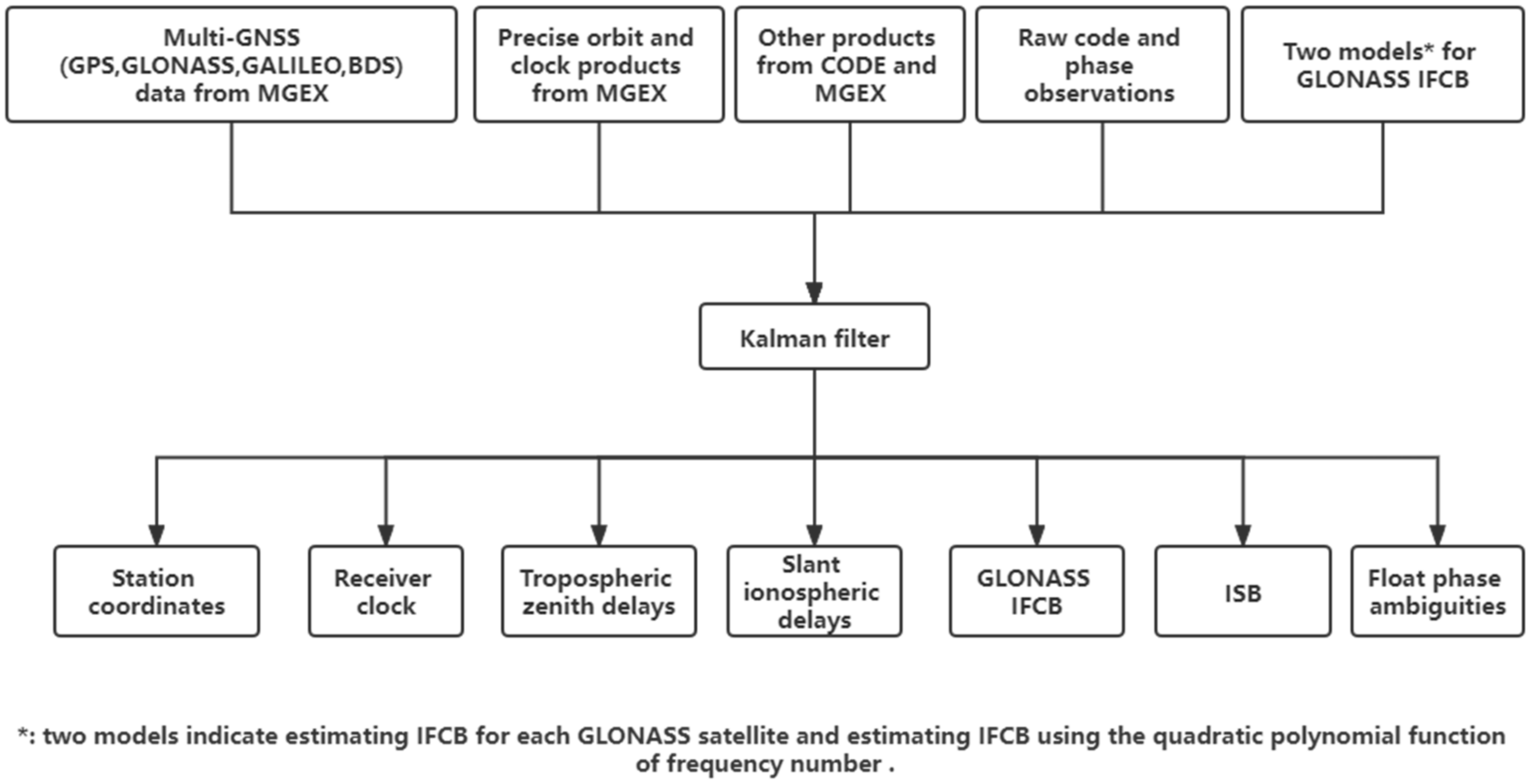
With this background, this study contributes a more comprehensive analysis that mainly focuses on the GLONASS IFCB models. First, we derive general PPP observation equations using undifferenced and uncombined observations. To obtain the full rank function model, we re-parameterize some unknown parameters. For the NF model, the GLONASS positioning model is essentially identical to the positioning models of GPS, BDS, or GALILEO. However, the IFCB is not fully absorbed by the receiver clock offset and ionospheric delay parameters. The remaining frequency-dependent IFCB is reflected in the pseudorange residuals, which causes many observations to be discarded as gross errors due to the large residuals. Consequently, the NF model that ignores the effects of IFCB is the worst. In addition to the NF model, there are only three commonly used IFCB models: the EG model, the QF model, and the LF model. Second, two relatively better models are identified from the remaining three models, and then, the two remaining IFCB models are introduced in detail. Third, detailed statistical analyses of the positioning accuracy, convergence speed, and data utilization are performed for the two remaining better IFCB models. Finally, the conclusions are provided.

2. Methods and Dataset

2.1. General Observation Models

The linearized raw observation equations of the pseudorange and carrier phase can be described as follows [32,33]:

$$p_{r,i}^{s,T}=u_r^{s,T}·x+c(d{t}_r-d{t}^{s,T})+{\gamma }_i^T·I_{r,1}^{s,T}+m·zw{d}_r+d_{r,i}^{s,T}-d_i^{s,T}+e_{r,i}^{s,T}$$

(1)

$$l_{r,i}^{s,T}=u_r^{s,T}·x+c(d{t}_r-d{t}^{s,T})-{\gamma }_i^T·I_{r,1}^{s,T}+m·zw{d}_r+{\lambda }_i^{s,T}·(N_{r,i}^{s,T}+D_{r,i}^{s,T}-D_i^{s,T})+{\xi }_{r,i}^{s,T}$$

(2)

where $s,T,r,i (i=1,2)$ denote the satellite number, satellite systems (GPS, BDS, GLONASS, and GALILEO), receiver, and carrier frequency band, respectively; $p_{r,i}^{s,T},l_{r,i}^{s,T}$ are the pseudorange and carrier phase observed values minus the computed values, respectively; $u_r^{s,T}$ denotes the unit vector from a satellite to the receiver; $x$ refers to the receiver position increment vector; $c$ is the speed of light in a vacuum; $d{t}^{s,T},d{t}_r$ are the satellite and receiver clock errors, respectively; $I_{r,1}^{s,T}$ is the slant ionospheric delay at frequency $f_1^{s,T}$; ${\gamma }_i^T={(f_1^{s,T})}^2/{(f_i^{s,T})}^2$ denotes the ionospheric factor at frequency band $i$; $m$ is the wet mapping function; $zw{d}_r$ is the zenith wet delay; ${\lambda }_i^{s,T}$ is the carrier phase wavelength; $N_{r,i}^{s,T}$ is the integer ambiguity at frequency band $i$; $d_{r,i}^{s,T},d_i^{s,T}$ are the receiver and satellite uncalibrated code delay (UCD) at frequency $f_i^{s,T}$, respectively; $D_{r,i}^{s,T},D_i^{s,T}$ are the receiver and satellite uncalibrated phase delay (UPD) at frequency $f_i^{s,T}$, respectively; $e_{r,i}^{s,T}$ refers to the sum of the observation noises for the pseudorange observations; ${\xi }_{r,i}^{s,T}$ is the sum of the observation noises for the carrier phase observations. To facilitate understanding, the following symbols are usually defined:

$$\left\{\begin{array}{c}{\alpha }_{m,n}^T=\frac{{(f_m^{s,T})}^2}{{(f_m^{s,T})}^2-{(f_n^{s,T})}^2}\\ {\beta }_{m,n}^T=\frac{-{(f_n^{s,T})}^2}{{(f_m^{s,T})}^2-{(f_n^{s,T})}^2}\\ DC{B}_{P_m{P}_n}^{s,T}=d_m^{s,T}-d_n^{s,T}\\ DC{B}_{r,P_m{P}_n}^{s,T}=d_{r,m}^{s,T}-d_{r,n}^{s,T}\\ d_{I{F}_{m,n}}^{s,T}={\alpha }_{m,n}^T·d_m^{s,T}+{\beta }_{m,n}^T·d_n^{s,T}\\ d_{r,I{F}_{m,n}}^{s,T}={\alpha }_{m,n}^T·d_{r,m}^{s,T}+{\beta }_{m,n}^T·d_{r,n}^{s,T}\end{array}\right.$$

(3)

Due to the use of precise satellite clock products in PPP, which is calculated from the IF model, the resulting satellite clock errors absorb the IF combination of the satellite UCD, as shown below [34]:

$$c·d{t}_{I{F}_{12}}^{s,T}=c·d{t}^{s,T}+({\alpha }_{12}^T·d_1^{s,T}+{\beta }_{12}^T·d_2^{s,T})=c·d{t}^{s,T}+d_{I{F}_{12}}^{s,T}$$

(4)

where $d{t}_{I{F}_{12}}^{s,T}$ is the precise clock correction provided by one of the analysis centers. Substituting Equations (3) and (4) into Equations (1) and (2) yields:

$$p_{r,1}^{s,T}=u_r^{s,T}·x+c·d{t}_r+d_{r,1}^{s,T}+m·zw{d}_r+I_{r,1}^{s,T}-{\beta }_{12}^T·DC{B}_{P_1{P}_2}^{s,T}+e_{r,1}^{s,T}$$

(5)

$$l_{r,1}^{s,T}=u_r^{s,T}·x+c·d{t}_r-I_{r,1}^{s,T}+m·zw{d}_r+d_{I{F}_{12}}^{s,T}+{\lambda }_1^{s,T}·(N_{r,1}^{s,T}+D_{r,1}^{s,T}-D_1^{s,T})+{\xi }_{r,1}^{s,T}$$

(6)

$$p_{r,2}^{s,T}=u_r^{s,T}·x+c·d{t}_r+d_{r,2}^{s,T}+m·zw{d}_r+{\gamma }_2^T·I_{r,1}^{s,T}+{\alpha }_{12}^T·DC{B}_{P_1{P}_2}^{s,T}+e_{r,2}^{s,T}$$

(7)

$$l_{r,2}^{s,T}=u_r^{s,T}·x+c·d{t}_r-{\gamma }_2^T·I_{r,1}^{s,T}+m·zw{d}_r+d_{I{F}_{12}}^{s,T}+{\lambda }_2^{s,T}·(N_{r,2}^{s,T}+D_{r,2}^{s,T}-D_2^{s,T})+{\xi }_{r,2}^{s,T}$$

(8)

2.2. Inter-System Bias (ISB)

When performing multi-GNSS PPP, it is necessary to consider the inter-system bias (ISB) among different satellite systems. ISB can be regarded as the difference in the receiver clock errors of different satellite systems [11]. This requires a satellite system to be selected as a reference. For example, based on GPS, the ISB parameters of GLONASS satellites are

$$IS{B}_r^R=c·(T^R-T^G)+(d_{r,IF}^R-d_{r,IF}^G)$$

(9)

where $IS{B}_r^R$ is the GLONASS ISB parameter; $T^R,T^G$ are the time references of the GLONASS and GPS systems, respectively; and $d_{r,IF}^R,d_{r,IF}^G$ are the IF combinations of the UCDs at the receiver ends. In this paper, only one ISB parameter is set to enhance the strength of the model, i.e., if one satellite system is selected as the reference, the ISB is introduced for all remaining satellite systems when they all use the receiver clock offset of the reference satellite system [35].

2.3. IFCB Models

This section compares the remaining three IFCB models (EG, QF, and LF models). The NF model, which ignores the effects of IFCB, has been eliminated in the Introduction chapter. We will choose two better models from these three remaining models and then compare the two selected models in all aspects to determine the best model.

Excluding the NF model that ignores the influence of IFCB, the remaining models include the LF model, which models IFCB as a linear function of the frequency channel, the QF model, which models IFCB as a quadratic polynomial function of the frequency channel, and the EG model, which estimates IFCB for each GLONASS satellite. To find the best IFCB model, we first compare the LF model with the QF model. The QF model is considered to be superior to the LF model in a previous study [31]. However, they only provided the analyses of GLONASS and GPS/GLONASS. We now draw conclusions from the principle.

2.3.1. LF Model

This model can be expressed as follows:

$$d_{r,i}^{s,R}=d_{r,i}^R+K^{s,R}·{\Delta }_{r,i}^R$$

(10)

where $d_{r,i}^R$ is the IFCB for the satellite whose frequency channel is 0, $K^{s,R}$ denotes the frequency channel (from −7 to 6) of satellite i, and ${\Delta }_{r,i}^R$ is the part of the IFCB that depends on the frequency channel.

2.3.2. QF Model

This model can be expressed as

$$d_{r,i}^{s,R}=d_{r,i}^R+K^{s,R}·{\Delta }_{r,i}^R+{(K^{s,R})}^2·{\Omega }_{r,i}^R$$

(11)

where $d_{r,i}^R,K^{s,R},{\Delta }_{r,i}^R$ have the same meaning as they do in Equation (10); ${\Omega }_{r,i}^R$ is part of the IFCB that quadratically depends on the frequency channel. It is clear that Equations (10) and (11) are special cases of the following polynomial function:

$${\displaystyle \sum _{i=0}^m{a}_i{x}^i}=a_0+a_{1}x+a_2{x}^2+\dots +a_m{x}^m$$

(12)

where $a_i$ is the polynomial coefficient, $x^i$ is the known observed value, and m is the order of the polynomial. If we consider $K$ in Equations (10) and (11) as $x$ in Equation (12), and similarly consider $d_{r,i}^R,{\Delta }_{r,i}^R,{\Omega }_{r,i}^R$ in Equations (10) and (11) as $a_i$ in Equation (12), then Equations (10) and (11) are special cases of Equation (12). The difference between Equation (10) and Equation (11) is that they have different degrees of order. Now, the problem translates into whether it is better to use a high-degree polynomial to estimate observations or a low-degree polynomial to estimate observations in mathematics.

From a mathematical point of view, we know that a quadratic function can be used to fit data conforming to a linear function, except that the coefficient of the quadratic term is very small during the fitting process. However, a linear function cannot fit data that conform to the quadratic function because the high-order coefficients that dominate the data trend do not exist and will cause a large error. Due to the influence of antennas and other factors, the IFCB of some stations meets the LF model, and some IFCB meets the QF model. For the IFCB that satisfies the LF model, if the QF model is used for estimation, the coefficient of the quadratic term tends to zero. The drawback of this approach is that the accuracy may not be as good as the IFCB estimated by the LF model, but it will not cause large errors. However, if the IFCB of some stations satisfies the QF model, but we use the LF model for fitting, then a large error will result because the high-order coefficients that dominate the data trend do not exist. Underfitting leads to errors, but overfitting leads to fitting curve oscillation and sensitivity to noise data. The method of increasing the dataset, which is easy for satellite positioning, can be used to solve the problem of fitting curve oscillation caused by overfitting [36]. The actual performance of these two IFCB models will be compared in the following Section 3.1 and Section 3.2 by considering actual data. Currently, only two models, the EG and QF models, are left to find the best method to estimate the IFCB.

2.3.3. EG Model

This model can be expressed as

$$d_{r,i}^{s,R}=d_{r,i}^R+{\varphi }_{r,i}^{s,R}$$

(13)

where $d_{r,i}^R$ has the same meaning as it does in Equation (10) and ${\varphi }_{r,i}^{s,R}$ denotes the part of the IFCB that depends on GLONASS satellite PRNs and their frequency. Moreover, in this model, the ISB and IFB parameters are highly correlated. To avoid this strong correlation, for each GLONASS satellite in PPP, the ISB and IFCB are combined into one parameter, ISFB, for estimation. Substituting Equations (9) and (13) into Equations (5)–(8) and re-parameterizing yield the equations below:

$$\{\begin{array}{c}c·d{\overline{t}}_r^T=c·d{t}_r+d_{r,I{F}_{12}}^T\\ ISF{B}_{r,12}^{s,R}={\varphi }_{r,2}^{s,R}-{\gamma }_2^R·{\varphi }_{r,1}^{s,R}+IS{B}_r^M\\ {\overline{I}}_{r,1}^{s,C}=I_{r,1}^{s,C}+{\beta }_{12}^C·DC{B}_{r,P_1{P}_2}^C\\ {\overline{I}}_{r,1}^{s,R}=I_{r,1}^{s,R}+{\beta }_{12}^R·DC{B}_{r,P_1{P}_2}^R+{\varphi }_{r,1}^{s,R}\\ {\overline{N}}_{r,1}^{s,C}={\lambda }_1^C·(N_{r,1}^{s,C}+D_{r,1}^C-D_1^{s,C})+d_{I{F}_{12}}^{s,C}-d_{r,I{F}_{12}}^C+{\beta }_{12}^C·DC{B}_{r,P_1{P}_2}^C\\ {\overline{N}}_{r,2}^{s,C}={\lambda }_2^C·(N_{r,2}^{s,C}+D_{r,2}^C-D_2^{s,C})+d_{I{F}_{12}}^{s,C}-d_{r,I{F}_{12}}^C+{\gamma }_2^C·{\beta }_{12}^C·DC{B}_{r,P_1{P}_2}^C\\ {\overline{N}}_{r,1}^{s,R}={\lambda }_1^{s,R}·(N_{r,1}^{s,R}+D_{r,1}^{s,R}-D_1^{s,R})+d_{I{F}_{12}}^{s,R}-d_{r,I{F}_{12}}^R+{\varphi }_{r,1}^{s,R}+{\beta }_{12}^R·DC{B}_{r,P_1{P}_2}^R\\ {\overline{N}}_{r,2}^{s,R}={\lambda }_2^{s,R}·(N_{r,2}^{s,R}+D_{r,2}^{s,R}-D_2^{s,R})+d_{I{F}_{12}}^{s,R}-d_{r,I{F}_{12}}^R+{\gamma }_2^R·{\varphi }_{r,1}^{s,R}+{\gamma }_2^R·{\beta }_{12}^R·DC{B}_{r,P_1{P}_2}^R\end{array}$$

(14)

where $M$ is the remaining satellite signals when one satellite signal is selected as the reference, $IS{B}_r^M$ is the ISB parameter for all remaining satellite systems, and capital $C$ is the satellite system using CDMA technology such as GPS, BDS, and GALILEO.

The QF model is described in Section 2.3.2. Substituting Equations (9) and (11) into Equations (5)–(8) and re-parameterizing yield the equations below:

$$\{\begin{array}{c}c·d{\overline{t}}_r^T=c·d{t}_r+d_{r,I{F}_{12}}^T\\ \begin{array}{l}{\Delta }_{r,12}^R={\Delta }_{r,2}^R-{\gamma }_2^R·{\Delta }_{r,1}^R\\ {\Omega }_{r,12}^R={\Omega }_{r,2}^R-{\gamma }_2^R·{\Omega }_{r,1}^R\end{array}\\ {\overline{I}}_{r,1}^{s,C}=I_{r,1}^{s,C}+{\beta }_{12}^C·DC{B}_{r,P_1{P}_2}^C\\ {\overline{I}}_{r,1}^{s,R}=I_{r,1}^{s,R}+{\beta }_{12}^R·DC{B}_{r,P_1{P}_2}^R+K^{s,R}·{\Delta }_{r,1}^R+{(K^{s,R})}^2·{\Omega }_{r,1}^R\\ {\overline{N}}_{r,1}^{s,C}={\lambda }_1^C·(N_{r,1}^{s,C}+D_{r,1}^C-D_1^{s,C})+d_{I{F}_{12}}^{s,C}-d_{r,I{F}_{12}}^C+{\beta }_{12}^C·DC{B}_{r,P_1{P}_2}^C\\ {\overline{N}}_{r,2}^{s,C}={\lambda }_2^C·(N_{r,2}^{s,C}+D_{r,2}^C-D_2^{s,C})+d_{I{F}_{12}}^{s,C}-d_{r,I{F}_{12}}^C+{\gamma }_2^C·{\beta }_{12}^C·DC{B}_{r,P_1{P}_2}^C\\ \begin{array}{c}{\overline{N}}_{r,1}^{s,R}={\lambda }_1^{s,R}·(N_{r,1}^{s,R}+D_{r,1}^{s,R}-D_1^{s,R})+d_{I{F}_{12}}^{s,R}-d_{r,I{F}_{12}}^R\\ +K^{s,R}·{\Delta }_{r,1}^R+{(K^{s,R})}^2·{\Omega }_{r,1}^R+{\beta }_{12}^R·DC{B}_{r,P_1{P}_2}^R\end{array}\\ \begin{array}{c}{\overline{N}}_{r,2}^{s,R}={\lambda }_2^{s,R}·(N_{r,2}^{s,R}+D_{r,2}^{s,R}-D_2^{s,R})+d_{I{F}_{12}}^{s,R}-d_{r,I{F}_{12}}^R+\\ {\gamma }_2^R·K^{s,R}·{\Delta }_{r,1}^R+{\gamma }_2^R·{(K^{s,R})}^2·{\Omega }_{r,1}^R+{\gamma }_2^R·{\beta }_{12}^R·DC{B}_{r,P_1{P}_2}^R\end{array}\end{array}$$

(15)

The symbols M, C have the same meaning as they do in Equation (14).

2.4. Parameter Estimation

For the EG and QF models, the estimated parameters for each station include the increment of receiver position vector $x$, receiver clock error $d{\overline{t}}_r^T$, the $ISF{B}_{r,12}^{s,R}$ for the ISB and IFCB estimated for each GLONASS satellite, as shown in Equation (16), the $IS{B}_r^M$ for the remaining three systems, and the ${\Delta }_{r,12}^R,{\Omega }_{r,12}^R$ for the GLONASS IFCB estimated as the QF model, as shown in Equation (17), the tropospheric delay $ZTD$, the slant ionospheric delay ${\overline{I}}_{r,1}^{s,T}$, and the float ambiguity ${\overline{N}}_{r,i}^{s,T}$. Equation (16) includes all of the estimated parameters for the EG model, and Equation (17) includes all of the estimated parameters for the QF model.

$$X={[x,d{\overline{t}}_r^T,ISF{B}_{r,12}^{s,R},ZTD,{\overline{I}}_{r,1}^{s,T},{\overline{N}}_{r,i}^{s,T}]}^T$$

(16)

$$X={[x,d{\overline{t}}_r^T,{\Delta }_{r,12}^R,{\Omega }_{r,12}^R,IS{B}_r^M,ZTD,{\overline{I}}_{r,1}^{s,T},{\overline{N}}_{r,i}^{s,T}]}^T$$

(17)

where $X$ refers to the estimated parameter vector.

2.5. Data and Processing Strategies

2.5.1. Experimental Data

To conduct an overall analysis of these IFCB models, we select observations sampled in 30 s from 140 stations of the IGS network on 1–7 September 2021. Figure 1 displays the geographic distribution of the 140 selected stations.

2.5.2. Processing Strategies

Data processing and analysis were carried out by using self-developed C++ language programming software. This software was developed based on other mature, open-source software, such as RTKLIB, goGPS, PRIDE-PPPAR, and GAMP [37,38,39,40]. Figure 2 shows the flow chart of the PPP processing strategy.

Table 1. Detailed processing models and strategies applied for combined PPP.

Item	Models/Strategy
Constellations	GPS, GLONASS, BDS, GALILEO
Observations	Raw code and phase observations
Estimator	Extended Kalman filter
Sampling rate	30 s
Elevation cut off angle	7°
Weighing strategy	A priori precision of 0.003 and 0.6 m for raw phase and code; Elevation-dependent weighing (1 for E > 30° otherwise 2 × sin(E)) is used
Receiver phase center	Corrected with the values from MGEX
Satellite phase center	Corrected with the values from MGEX
Phase windup	Corrected
Relativistic effect	Relativistic models
Sagnac effect	Corrected
Tidal effects	Consider solid tides, ocean loading, and polar tides
Satellite orbit and clock	precise products from MGEX
Differential code bias	using MGEX DCB products
Receiver clock offset	Set up for GPS and estimated as white noise
Receiver ISB	estimated as 1-day constants
Station coordinates	Estimated as constants/white noises in static/kinematic modes
Zenith tropospheric delay	ZTD estimation; Estimated as random-walk noise (1.0 × 10−4 m/sqrt(s)); GMF is used
Slant ionospheric delay	Estimated using two frequencies; Estimated as random walk (4 × 10−2 m/sqrt(s))
Phase ambiguities	Estimated as float constants for each arc
GLONASS IFCB	estimating IFCB for each GLONASS satellite and modelling IFCB as a quadratic function of frequency channels

lists the detailed processing models and strategies applied for combined PPP.

3. Results and Analyses

3.1. Positioning Accuracy

In this section, we analyze all the combinations, including the GLONASS data, from the perspective of positioning accuracy. The accuracy of each combination is the average accuracy of all selected stations. The positioning accuracy is assessed through a comparison with IGS weekly solutions.

Figure 3, Figure 4, Figure 5 and Figure 6 show the positioning accuracies of different combined solutions using the NF model, LF model, QF model, and EG model for all IGS selected stations in static mode. The abbreviations G, B, R, and E denote GPS, BDS, GLONASS, and GALILEO, respectively. G/R, R/B, R/E, G/R/B, G/R/E, R/B/E, and G/R/B/E denote the GPS/GLONASS, GLONASS/BDS, GLONASS/GALILEO, GPS/GLONASS/BDS, GPS/GLONASS/GALILEO, GLONASS/BDS/GALILEO, and GPS/GLONASS/BDS/GALILEO, respectively. In each figure, the positioning accuracies of different combined solutions are not very different in the three directions using the one-week observation data. Figure 3, Figure 4, Figure 5 and Figure 6 demonstrate that the positioning accuracies of the same combination for these four IFCB models in static mode are comparable in three directions for the one-week observation data. The highest accuracy in each figure is approximately 0.4 cm in the N direction, followed by approximately 0.5 cm in the E direction, and the lowest accuracy is approximately 1.2 cm in the U direction. Figure 7, Figure 8, Figure 9 and Figure 10 show the positioning accuracy of different combined solutions using the NF model, LF model, QF model, and EG model for all stations in kinematic mode. The positioning accuracies of different combined solutions are very different in the three directions for each figure. This is mainly because, in kinematic mode, the station coordinates are estimated as white noise, unlike those in static mode that are estimated as constants. The positioning accuracies of the same combination for these four IFCB models are almost the same in the E, N, and U directions using the one-week observation data. In kinematic mode, the average accuracies of all different combinations for these four IFCB models in the E, N, and U directions are 4.4, 2.5, and 6.7 cm, respectively. However, for GLONASS-only, the accuracy of the EG model in the N direction is the worst among all the IFCB models. There are two possible reasons for the anomalous accuracy of the EG model in the N direction, the first being that the station coordinates are estimated as random noise in the kinematic mode, and the second being that the number of observed equations using only GLONASS data is relatively small and that the EG model greatly increases the number of parameters being estimated, thus affecting the accuracy of the solution. Figure 3, Figure 4, Figure 5, Figure 6, Figure 7, Figure 8, Figure 9 and Figure 10 also reveal that the combined systems with GPS data have better positioning results than other combined systems for both static and kinematic modes. In static mode, the average accuracies in the E, N, and U directions are 0.4, 0.4, and 1.0 cm for the combinations that contain the GPS data, respectively, and 0.5, 0.4, and 1.1 cm for the combinations that do not contain the GPS data, respectively. In kinematic mode, the average accuracies in the E, N, and U directions are 2.3, 2.0, and 5.4 cm for the combinations that contain the GPS data, respectively, and 6.4, 3.1, and 8.6 cm for the combinations that do not contain the GPS data, respectively. The foremost reason is that the stations that can receive GPS signals are most widely distributed, and the GPS signal processing models are much more complete than the models for other systems. These results make the combined solutions meaningful because the combination of different systems can improve the positioning accuracy, especially in kinematic mode.

3.2. Convergence Time

To compare the effectiveness of these IFCB models for different combinations, we comprehensively measure their convergence time for different combinations. We define the PPP performance as the time taken for 68% and 95% of all stations to reach the specified accuracy and retain this accuracy for 20 sequence epochs. For static PPP, the specified accuracy is 2 cm for the E, N, and U components; for kinematic PPP, the specified accuracy is 10 cm for the E, N, and U components.

To purely compare the performances of the NF, LF, and QF models, we only analyze the convergence time of these three models in combination R to identify the best model.

Table 2. Convergence times of the NF model, LF model, and the QF model in combination R (unit: min).

		Static			Kinematic
		E	N	U	E	N	U
68%	NF	116	67	97	109	84	175
	LF	89	50	73	115	68	142
	QF	86	50	73	110	71	132
95%	NF	298	126	244	207	178	374
	LF	241	92	244	187	144	250
	QF	170	97	159	185	139	249
DAE2	LF	63	81	244	78	61	81
	QF	63	81	244	61	30	62
LPGS	LF	106	106	102	236	264	269
	QF	97	93	97	233	264	269

shows the convergence times of the NF model, LF model, and QF model in the three directions under static and kinematic conditions. In the table, 68% and 95% represent the time required for 68% and 95% of the total stations to reach the convergence accuracy in three directions, respectively. The receiver of station DAE2 is Trimble NetR9, and its IFCB satisfies the LF model according to Shi’s article; the receiver of station LPGS is JAVAD TRE_G3 DELTA, and its IFCB satisfies the QF model according to Shi’s article [30]. Table 2 shows that, overall, the convergence time of the LF model is better than that of the NF model. For 68% of the total stations, compared to those of the NF model, the convergence times of the LF model are improved by 23%, 25%, and 24% in the E, N, and U directions in the static case, respectively, and by −6%, 20%, and 19% in the kinematic case, respectively; for 95% of the total stations, the improvements are 19%, 27%, and 0% in the static case, and 10%, 19%, and 33% in the kinematic case. Overall, the convergence time of the QF model is better than that of the LF model. For 68% of the total stations, compared to those of the LF model, the convergence times of the QF model are improved by 3%, 0%, and 0% in the E, N, and U directions in the static case, respectively, and by 4%, −4%, and 7% in the kinematic case, respectively; for 95% of the total stations, the improvements are 29%, −5%, and 36% in the static case, and 1%, 3%, and 0.4% in the kinematic case. For station DAE2, even if its IFCB satisfies the LF model, the convergence times of the LF and QF models are comparable in the static case, and the convergence times of the QF model in the kinematic case are improved by 24%, 51%, and 23% in the E, N, and U directions, respectively, compared to those of the LF model. For station LPGS, even if its IFCB satisfies the QF model, the convergence times of the QF model in the static case are improved by 8%, 12%, and 5% in the E, N, and U directions, respectively, compared to those of the LF model, and the convergence time of the LF and QF models are comparable in the kinematic case. This indicates that the QF model can also be used to estimate the IFCB, satisfying the LF model well. The results in Table 2 also prove the contents of Section 2.3.2.

Now, the two remaining better IFCB models are the QF model and the EG model. To determine the best model for estimating IFCB, the following will compare these two IFCB models in various aspects.

Table 3. Convergence time of the EG method (unit: min) (R).

	Static PPP			Kinematic PPP
	E	N	U	E	N	U
68%	73	39	85	99	61	132
95%	153	83	163	158	125	232

,

Table 4. Convergence time of the QF method (unit: min) (R).

	Static PPP			Kinematic PPP
	E	N	U	E	N	U
68%	86	50	74	110	75	132
95%	170	102	159	185	139	249

,

Table 5. Convergence time of the EG method (unit: min) (G/R).

	Static PPP			Kinematic PPP
	E	N	U	E	N	U
68%	44	28	66	20	9	24
95%	99	51	163	47	20	39

,

Table 6. Convergence time of the QF method (unit: min) (G/R).

	Static PPP			Kinematic PPP
	E	N	U	E	N	U
68%	43	28	59	21	9	23
95%	148	67	165	47	20	40

,

Table 7. Convergence time of the EG method (unit: min) (R/B).

	Static PPP			Kinematic PPP
	E	N	U	E	N	U
68%	108	58	107	74	40	80
95%	216	202	250	170	105	279

,

Table 8. Convergence time of the QF method (unit: min) (R/B).

	Static PPP			Kinematic PPP
	E	N	U	E	N	U
68%	95	53	88	68	36	60
95%	149	141	229	130	72	147

,

Table 9. Convergence time of the EG method (unit: min) (R/E).

	Static PPP			Kinematic PPP
	E	N	U	E	N	U
68%	88	43	95	35	24	57
95%	196	115	329	163	146	347

,

Table 10. Convergence time of the QF method (unit: min) (R/E).

	Static PPP			Kinematic PPP
	E	N	U	E	N	U
68%	72	41	79	39	17	49
95%	210	88	233	127	32	110

,

Table 11. Convergence time of the EG method (unit: min) (G/R/B).

	Static PPP			Kinematic PPP
	E	N	U	E	N	U
68%	42	29	60	21	8	26
95%	99	69	157	36	16	39

,

Table 12. Convergence time of the QF method (unit: min) (G/R/B).

	Static PPP			Kinematic PPP
	E	N	U	E	N	U
68%	43	29	62	22	9	24
95%	149	69	156	41	17	41

,

Table 13. Convergence time of the EG method (unit: min) (G/R/E).

	Static PPP			Kinematic PPP
	E	N	U	E	N	U
68%	47	31	64	16	6	17
95%	127	56	164	34	14	49

,

Table 14. Convergence time of the QF method (unit: min) (G/R/E).

	Static PPP			Kinematic PPP
	E	N	U	E	N	U
68%	44	28	62	18	8	20
95%	145	50	164	35	14	49

,

Table 15. Convergence time of the EG method (unit: min) (R/B/E).

	Static PPP			Kinematic PPP
	E	N	U	E	N	U
68%	87	46	106	54	25	55
95%	154	122	269	163	94	161

,

Table 16. Convergence time of the QF method (unit: min) (R/B/E).

	Static PPP			Kinematic PPP
	E	N	U	E	N	U
68%	84	38	84	42	15	46
95%	154	105	172	93	38	90

,

Table 17. Convergence time of the EG method (unit: min) (G/R/B/E).

	Static PPP			Kinematic PPP
	E	N	U	E	N	U
68%	49	30	77	19	7	20
95%	125	67	171	37	14	45

and

Table 18. Convergence time of the QF method (unit: min) (G/R/B/E).

	Static PPP			Kinematic PPP
	E	N	U	E	N	U
68%	50	29	77	19	9	20
95%	145	56	171	41	13	45

present the convergence time for all combinations, including the GLONASS data. All tables show that the convergence times of the EG and QF models have no obvious law under the same convergence evaluation conditions. For the GLONASS-only combination, when 68% of the total stations reach the convergence accuracy, compared to those of the QF model, the improvements of the convergence time for the EG model in the three directions are 15%, 20%, and −15% in static mode, and 10%, 19%, and 0% in kinematic mode; when 95% of the total stations reach the convergence accuracy, the improvements are 10%, 18%, and −3% in static mode, and 14%, 19%, and 6% in kinematic mode. For the combinations including GPS data, when 68% of the total stations reach the convergence accuracy, the performance of the EG model and that of the FQ model are roughly the same; when 95% of the total stations reach the convergence accuracy, the convergence time of the EG model in the E direction is better than that of the QF model, with the improvement being approximately 22%, and the convergence times in the N and U directions are roughly the same. The reason may be that GPS satellites are widely distributed around the world, and the number of GPS satellites that can be observed in each epoch is large and does not change much over time. This is beneficial for the EG model with many unknown parameters. For the remaining combinations, the convergence speed of the EG model is much slower than that of the QF model. When 68% of the total stations reach the convergence accuracy, compared with those of the EG model, the convergence speeds of the QF model in the E, N, and U directions are increased by 11%, 9%, and 18% in the static case, respectively, and 6%, 16%, and 18% in the kinematic case; when 95% of the total stations reach the convergence accuracy, the improvements are 8%, 22%, and 24% under static conditions and 29%, 54%, and 52% under kinematic conditions. This is mainly because the EG model greatly increases the number of estimated parameters, and these satellites are affected by factors such as geography and time, leading to a large variation in the number of available satellites that can be observed per epoch. As a result, the numerical solution is unstable. The above results show that the EG model converges slightly better than the QF model in some directions for some combinations, and the improvement rate does not exceed 22%. However, the QF model converges much faster than the EG model in some directions for some combinations, and the improvement rate in some directions is more than 50%. The experimental results also show that the convergence time of the EG model is shorter than that of the QF model in three directions for combination R, but the convergence time of the QF model is shorter than that of the EG model in three directions for the combination R/B. This means that the convergence time is related not only to the IFCB models, but also to the addition of other constellations.

To better investigate the convergence speeds of the two IFCB models (the EG and QF models) in three directions for different combinations, we studied the convergence time when the convergence accuracies of these two IFCB models in the three directions reached 0.02, 0.04, 0.06, 0.08, and 0.1 m in static mode and 0.05, 0.1, 0.15, 0.2, and 0.25 m in kinematic mode. Figure 11 shows the time required for 68% of the total stations to reach the convergence accuracy. Figure 12 shows the time required for 95% of the total stations to reach the convergence accuracy. Each picture includes four parts (a), (b), (c), and (d), and each part includes four subplots. It means that each figure includes 16 subplots. The left column of each part shows the convergence times of the two IFCB models in static mode with different convergence accuracy requirements, while the right column of each part shows the convergence times of the two IFCB models in kinematic mode with different convergence accuracy requirements. These two figures show that the convergence speed in the N direction is faster than that in the E and U directions for all combinations. The figures also show that, regardless of static or kinematic mode, when the accuracy threshold value is set relatively low, the convergence speeds of the two IFCB models for the same combination in the three directions are roughly the same. The convergence speed of the EG model in some directions for the combinations including the GPS data is slightly better than that of the QF model when the accuracy threshold value is set relatively high, but the improvement is limited. In other combinations, such as combination R/B or R/B/E, the EG model generally has a worse convergence speed than the QF model, and in some directions, the convergence speed of the QF model is much better than that of the EG model. This means that, although the EG model has slightly better convergence time in some directions for some combinations than the QF model, the improvement is limited. In the G/R combination, for example, the convergence time of the EG model is better than that of the QF model, which is consistent with the conclusions reported in a previous study [31]. In other combinations, the EG model lags far behind the QF model in some directions, such as the B/E combination. The reasons for this result are that the EG model greatly increases the number of unknown parameters, and the number and quality of observation satellites in the combinations without the GPS data are related to the geographical location of the station, receiving antennas, etc. Both of these reasons will have a great impact on the convergence time and accuracy of the solution.

3.3. Data Utilization

Since the Kalman filter is used in the calculation process, one solution should be obtained for each epoch. However, the experimental results show that the EG model cannot output solutions in some epochs for some combinations, while the QF model can almost provide output solutions for each combination in each epoch. Therefore, it is necessary to study the difference in data utilization between these two models (EG and QF models). In this paper, the data utilization is defined as the ratio of the number of solutions output by each station for both methods, and the QF method is used as a reference. In other words, data utilization is the ratio of the number of solutions of the EG method to the number of solutions of the QF method at each station.

Table 19. Data utilization of the EG model (based on the QF model).

Combinations	Static	Kinematic
R	99.99%	99.97%
G/R	100.00%	100.00%
R/B	84.86%	84.12%
R/E	94.14%	94.10%
G/R/B	99.90%	100.00%
G/R/E	100.00%	100.00%
R/B/E	99.24%	99.18%
G/R/B/E	100.00%	100.00%

gives the data utilization for each satellite combination. These data are the average data utilization of all stations. From these data, R/B has the lowest data utilization, followed by R/E, R/B/E, and R. However, in the combinations that contain GPS data, the data utilization is almost 100%. This is because the stations that can receive GPS signals are widely distributed around the world, and more GPS satellites can be observed in each epoch, which increases the number of observation equations and is good for the EG method with more unknown parameters. Thus, the data utilization values of these two IFCB methods are approximately the same. However, in the combinations that do not contain GPS data, the number of satellites is affected by time, geography, and receiver antennas, and the EG model has more parameters to be estimated than the QF model. These reasons lead to the EG model not being able to output solutions in some epochs, so the data utilization rate decreases.

4. Discussion

This paper discussed four IFCB models, among which two poor models are eliminated through theoretical analysis at the very beginning. The remaining two methods are studied in detail in terms of positioning accuracy, convergence time, and data utilization. In some combinations, such as G/R and R, the convergence time of the EG model is comparable to that of the QF model and, in some directions, is even slightly better than that of the QF model. These results are consistent with previous research results [31]. However, for other combinations, such as R/B, the convergence time of the QF model is much better than that of the EG model. The main reason is that the EG model has too many unknown parameters, and the number of available satellites is sometimes too small for some combinations. Due to the geometric distribution of some satellite systems (BDS, GLONASS, and GALILEO) and the problems of IGS station receiver antennas, many stations cannot receive a sufficient number of satellites, which is the main factor leading to the different performances of the two IFCB models. From the above, we can infer that when the receiver can receive more satellites from any satellite system in the future and the error models of these satellites can be well corrected, the accuracy of the EG model may be as good as that of the QF model. In the next step, the main research direction is to fix the ambiguity of GLONASS with the addition of IFCB correction.

5. Conclusions

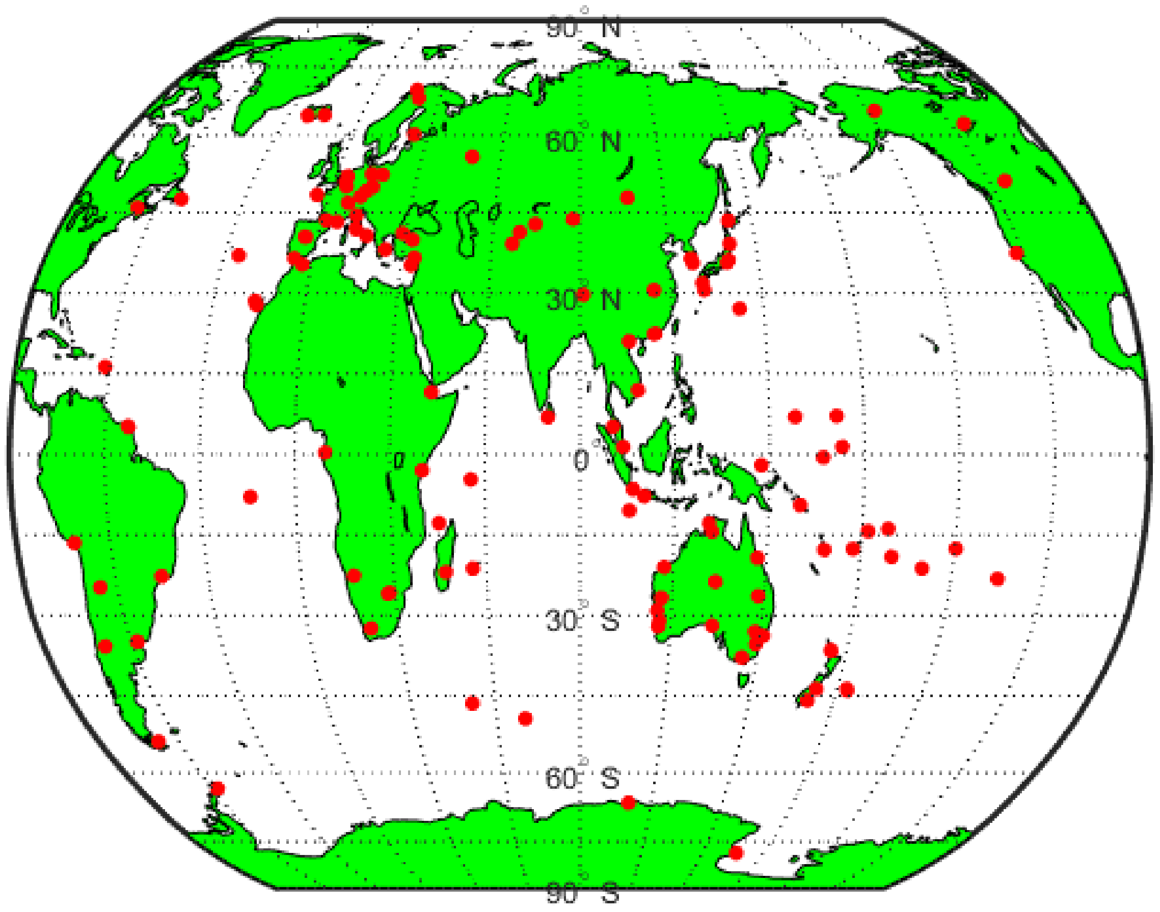
This paper provides a much more detailed analysis of the two IFCB models for combined PPP. We first propose a universal PPP model that uses raw pseudorange and carrier phase observations instead of other combined observations to amplify noise errors. In this model, two better IFCB handling schemes, the EG and QF schemes, from the four commonly used schemes are comprehensively compared and analyzed. To obtain the full-rank function model, we recombine the unknown parameters. The data from 140 IGS stations obtained between 1–7 September 2021 are used to validate the feasibility of these proposed IFCB models, and the results are presented.

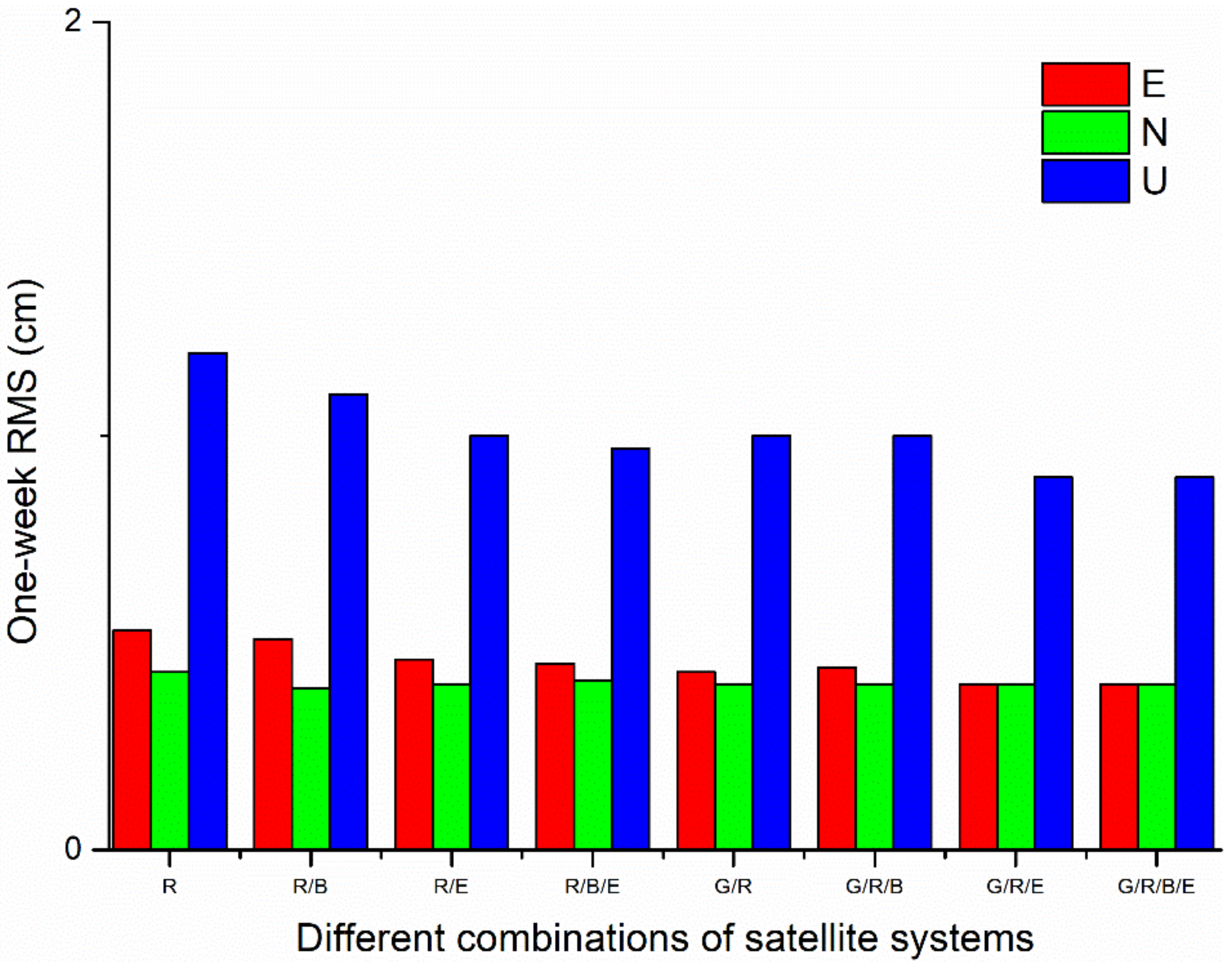
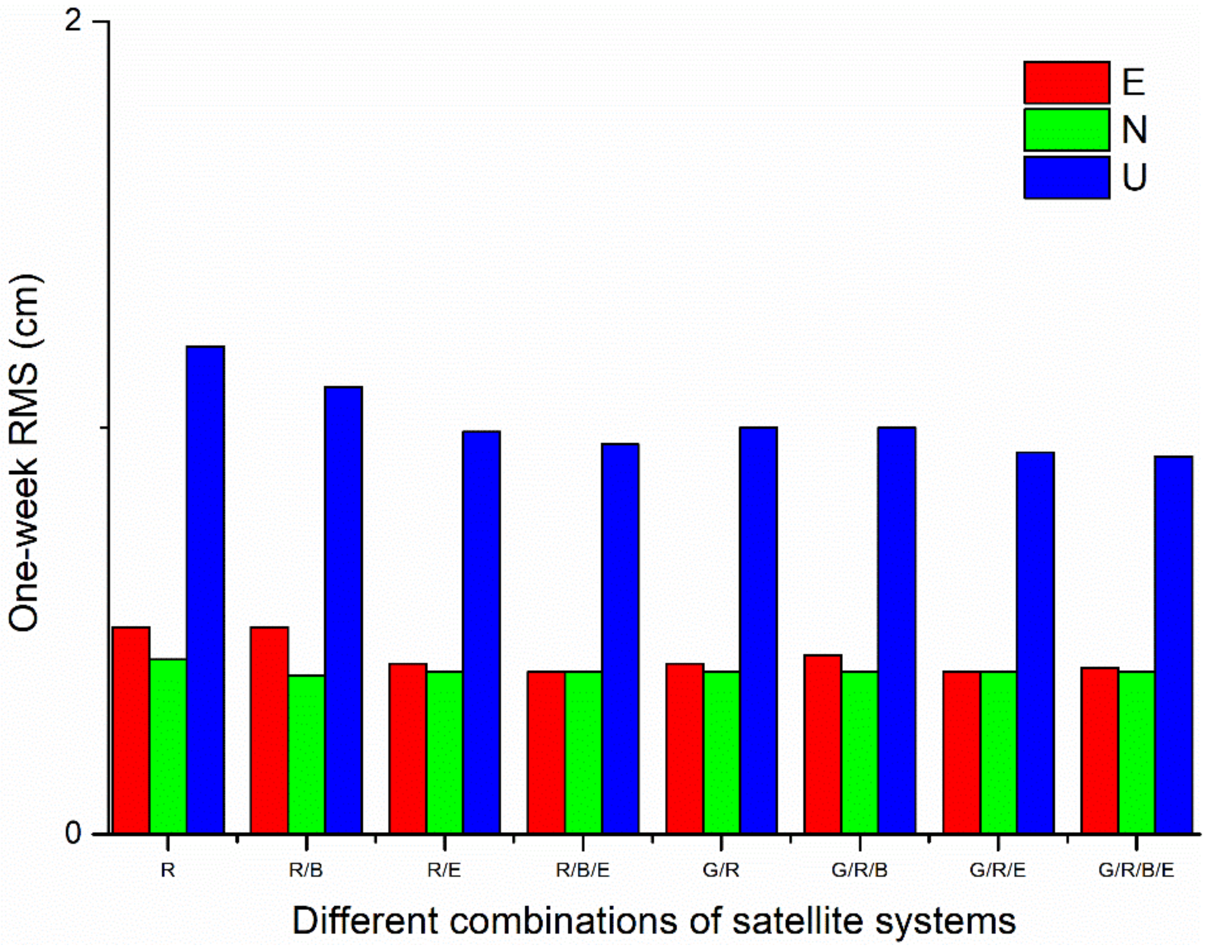
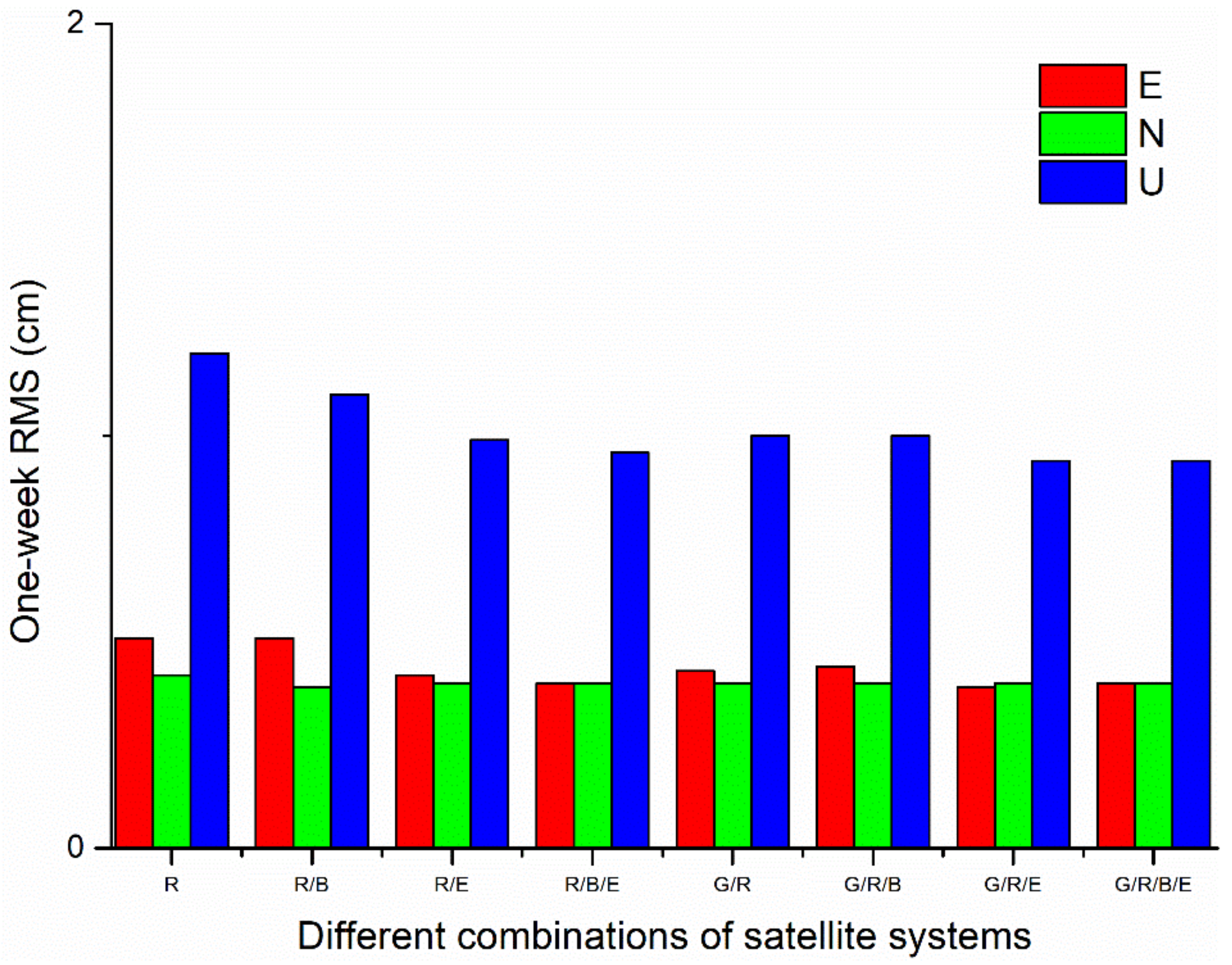
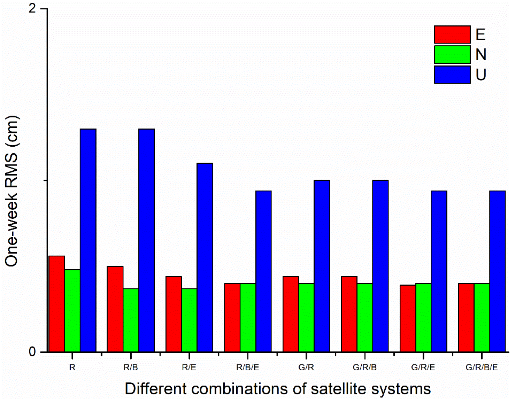
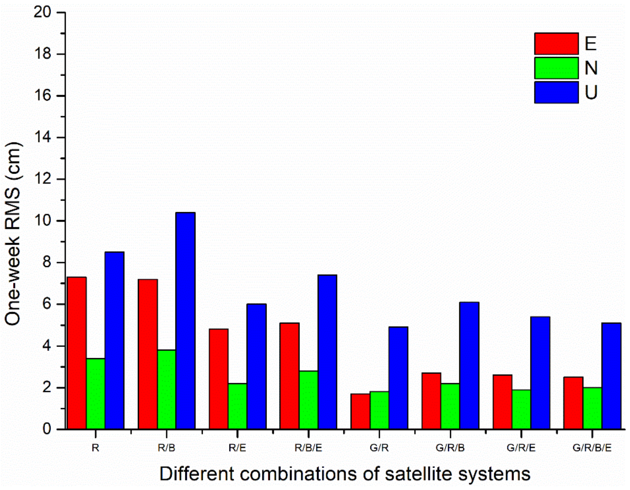
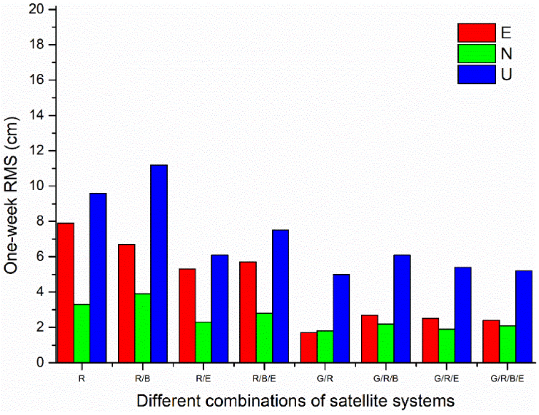
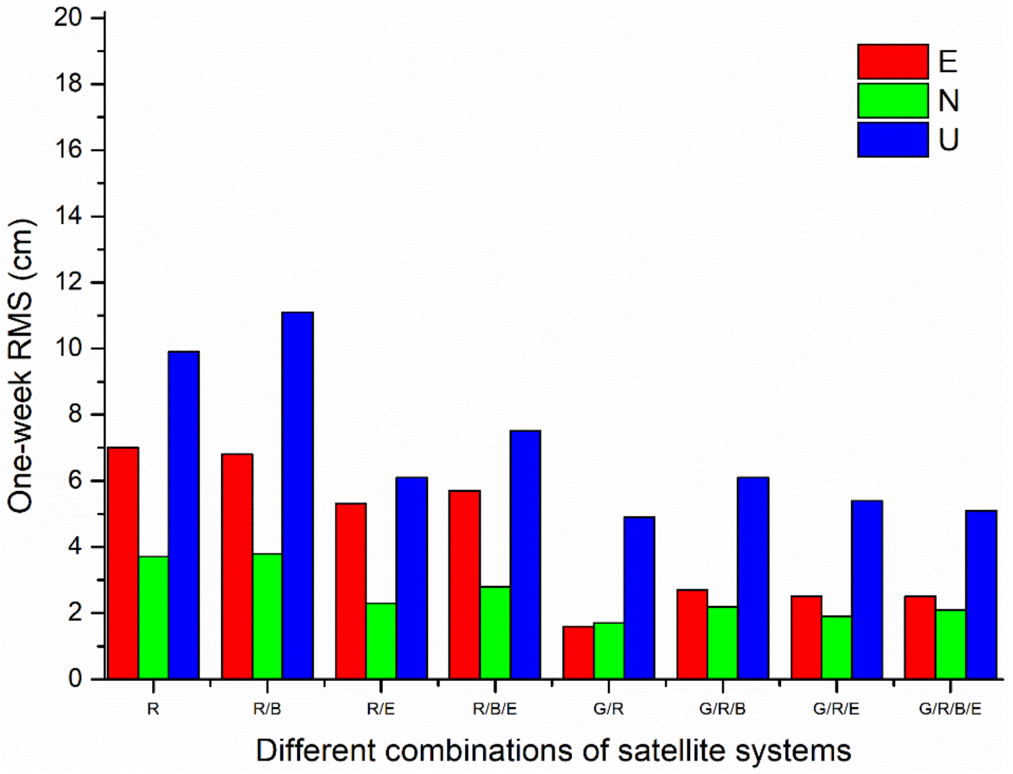
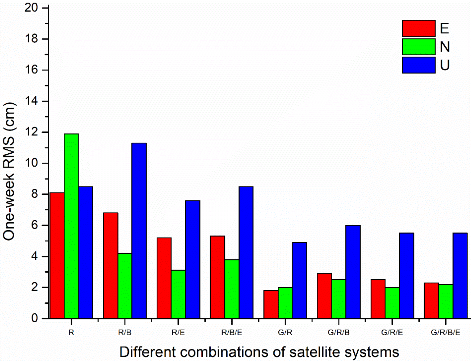
First, the positioning accuracy of four IFCB models for different combined solutions is analyzed in both static and kinematic modes with respect to the IGS weekly solutions. The positioning accuracies of different combined solutions for the same IFCB model are not very different in the three directions using the one-week observation data in static mode. The positioning accuracies of the same combination for these four IFCB models in static mode are also compatible in the three directions using the one-week observation data. In static mode, the average accuracies of the positioning results are 0.5, 0.4, and 1.2 cm in the E, N, and U directions, respectively. In kinematic mode, the positioning accuracies of different combined solutions are very different in the three directions for each IFCB model. However, the positioning accuracies of the same combination for these four IFCB models are almost the same in the E, N, and U directions using the one-week observation data. In kinematic mode, the average accuracies of the positioning results in the E, N, and U directions are 4.4, 2.5, and 6.7 cm, respectively. The results also reveal that the combinations with GPS data have better accuracy in three directions than other combinations in kinematic mode.

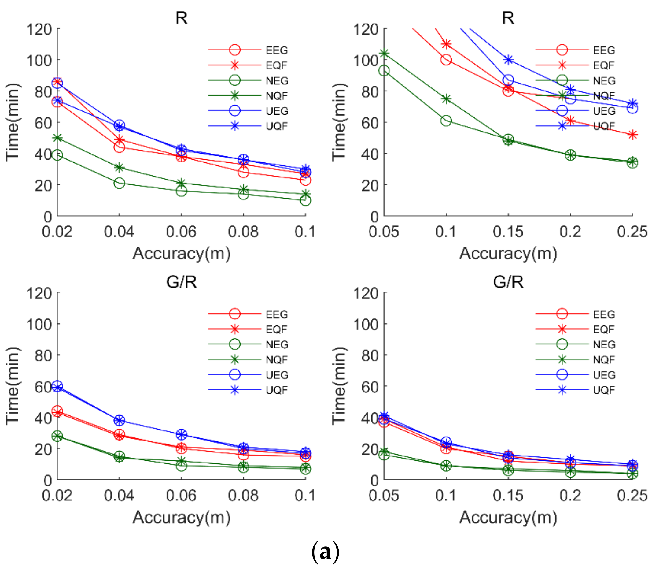
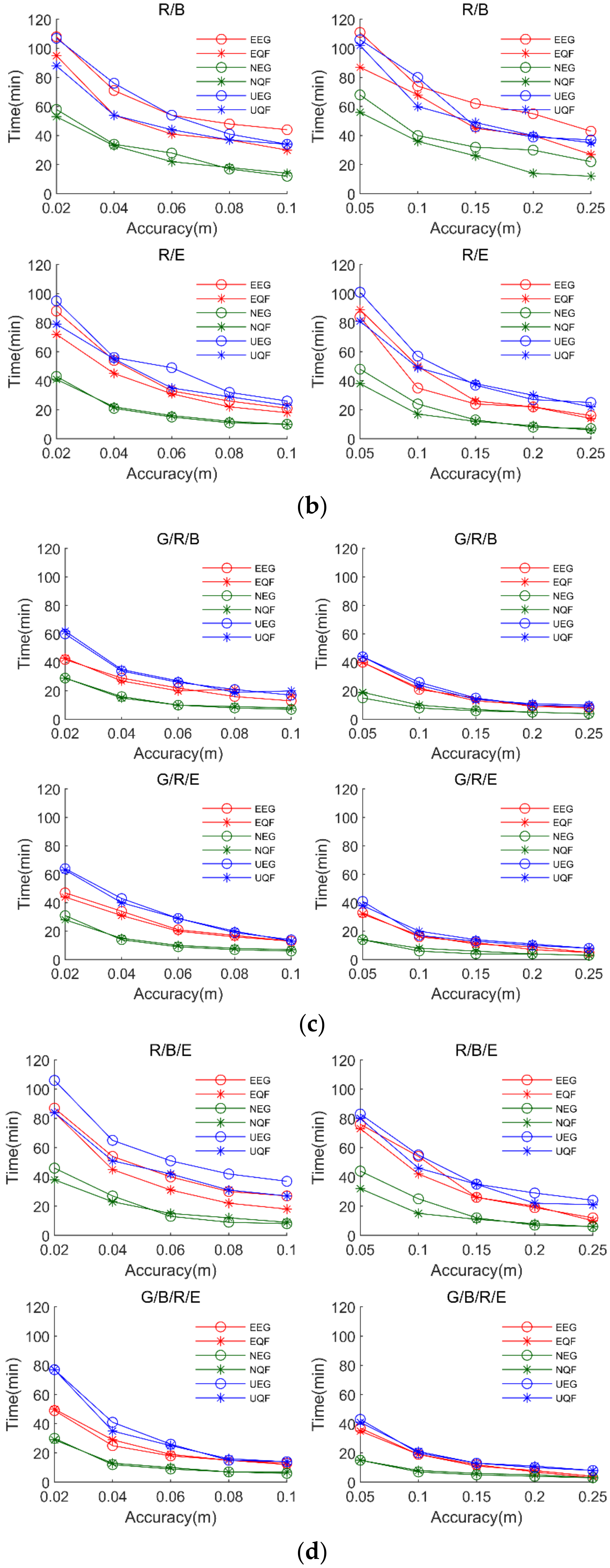
Second, the results show that the convergence time of the LF model overall is better than that of the NF model. For 68% of the total stations, compared to those of the NF model, the convergence times of the LF model in the E, N, and U directions are improved by 23%, 25%, and 24% in the static case, respectively, and by −6%, 20%, and 19% in the kinematic case, respectively; for 95% of the total stations, the improvements are 19%, 27%, and 0% in the static case, and 10%, 19%, and 33% in the kinematic case. For 68% of the total stations, compared to those of the LF model, the convergence times of the QF model in the E, N, and U directions are improved by 3%, 0%, and 0% in the static case, respectively, and by 4%, −4%, and 7% in the kinematic case, respectively; for 95% of the total stations, the improvements are 29%, −5%, and 36% in the static case, and 1%, 3%, and 0.4% in the kinematic case. The experimental results also show that the quadratic function can be used to estimate the IFCB regardless of whether the IFCB satisfies the primary function or the quadratic function.

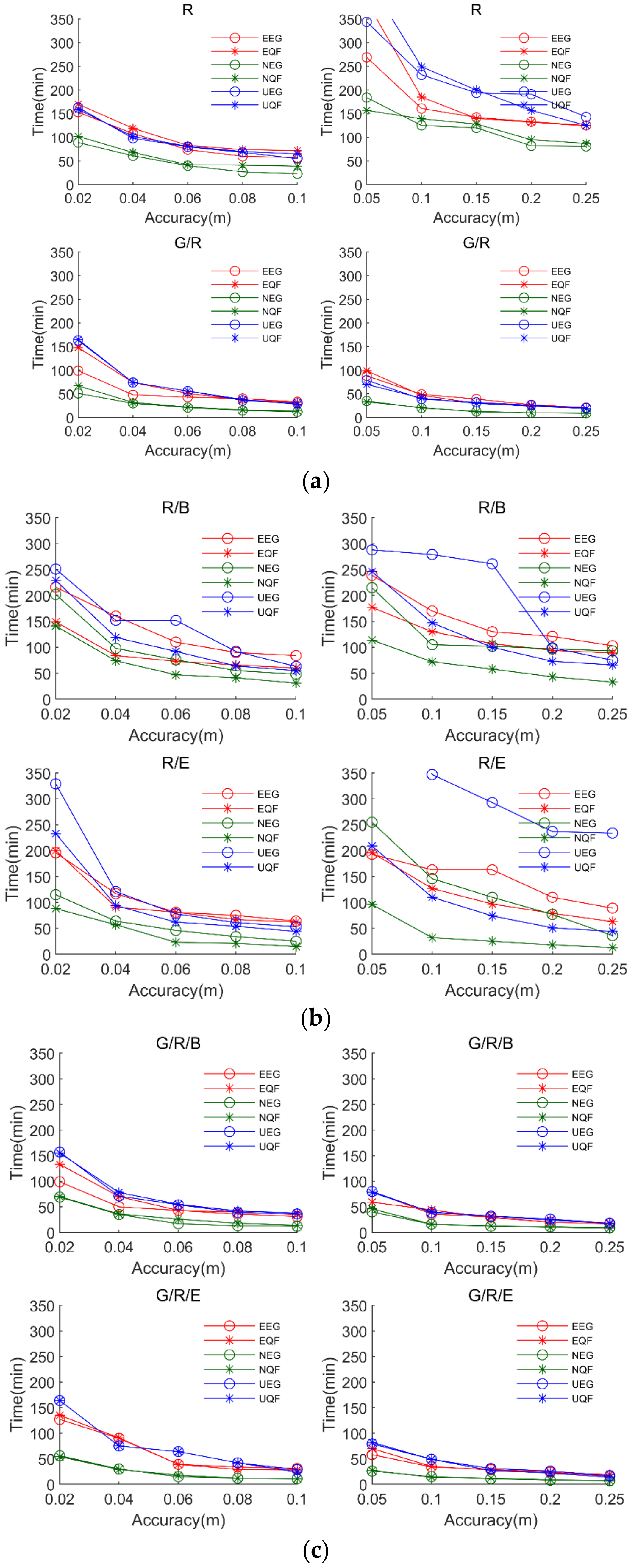
For the QF model and EG model, the convergence time of the EG model is better than that of the QF model for combinations such as GLONASS-only and GPS/GLONASS, which is consistent with the conclusions in the previous study [31], but the improvement rate does not exceed 22%. For the rest of the combinations that do not contain GPS data, the convergence speed of the QF model is much better than that of the EG model. The improvement rate in some directions is more than 50%. The results also show that the convergence time is related not only to the IFCB models, but also to the addition of other constellations. To better study the IFCB model, we study the convergence speed of the combined solutions with different accuracy thresholds. The results show that for some combinations, the EG models indeed converge slightly faster than QF models, but in some combinations, the QF models converge much faster than the EG models.

Third, in the combinations that contain GPS data, the EG model and QF model have almost the same data utilization in both static and kinematic modes, while in the combinations that do not contain GPS data, the data utilization of the EG model is less than that of the QF model in both static and kinematic modes. In summary, the EG model and the QF model can achieve the same accuracy in both static and kinematic modes after long-term observation. In some combinations, the convergence time of the EG model is better than that of the QF model in three directions, but the improvement is limited. In other combinations, the convergence time of the QF model is much better than that of the EG model in three directions. For the combinations including GPS data, the QF model and EG model have almost the same data utilization values; for the combinations not including GPS data, the QF model has higher data utilization than the EG models. Therefore, considering the positioning accuracy, convergence time, data utilization, and reliability of the function model, we suggest using the QF model to estimate IFCB.

References

1. Zumberge, J.F.; Heflin, M.B.; Jefferson, D.C.; Watkins, M.M.; Webb, F.H. Precise point positioning for the efficient and robust analysis of GPS data from large networks. J. Geophys. Res. 1997, 102, 5005–5017. [Google Scholar] [CrossRef] [Green Version]
2. Bisnath, S.; Gao, Y. Current state of precise point positioning and future prospects and limitations. IAG Symp. 2007, 133, 615–624. [Google Scholar]
3. Bock, Y.; Melgar, D. Physical applications of GPS geodesy: A review. Rep. Prog. Phys. 2016, 79, 106801. [Google Scholar] [CrossRef] [PubMed]
4. Yang, Y.; Li, J.; Xu, J.; Tang, J.; Guo, H.; He, H. Contribution of the compass satellite navigation system to global PNT users. Chin. Sci. Bull. 2011, 56, 2813–2819. [Google Scholar] [CrossRef] [Green Version]
5. Guo, F.; Li, X.; Zhang, X.; Wang, J. Assessment of precise orbit and clock products for GALILEO, Beidou, and QZSS from IGS Multi-GNSS Experiment (MGEX). GPS Solut. 2017, 21, 279–290. [Google Scholar] [CrossRef]
6. Montenbruck, O.; Steigenberger, P.; Prange, L.; Deng, Z.; Zhao, Q.; Perosanz, F.; Romero, I.; Noll, C.; Stürze, A.; Weber, G.; et al. The GNSS Experiment (MGEX) of the international GNSS service (IGS)—Achievements, prospects and challenges. Adv. Space Res. 2017, 59, 1671–1697. [Google Scholar] [CrossRef]
7. Li, X.; Li, X.; Yuan, Y.; Zhang, K.; Zhang, X.; Wickert, J. GNSS phase delay estimation and PPP ambiguity resolution: GPS, BDS, GLONASS, GALILEO. J. Geod. 2018, 92, 579–608. [Google Scholar] [CrossRef]
8. Li, X.; Li, X.; Liu, G.; Feng, G.; Yuan, Y.; Zhang, K.; Ren, X. Triple-frequency PPP ambiguity resolution with multi-constellation GNSS: BDS and Galileo. J. Geod. 2019, 93, 1105–1122. [Google Scholar] [CrossRef]
9. Ge, M.; Zhang, H.; Jia, X.; Song, S.; Wickert, J. What is achievable with the current compass constellation. GPS World 2012, 1, 29–34. [Google Scholar]
10. Li, X.; Ge, M.; Dai, X.; Ren, X.; Fritsche, M.; Wickert, J.; Schuh, H. Accuracy and reliability of multi-GNSS real-time precise positioning: GPS, GLONASS, BeiDou, and GALILEO. J. Geod. 2015, 89, 607–635. [Google Scholar] [CrossRef]
11. Lou, Y.; Zheng, F.; Gu, S.; Wang, C.; Guo, H.; Feng, Y. Multi-GNSS precise point positioning with raw single-frequency and dual frequency measurement models. GPS Solut. 2016, 20, 849–862. [Google Scholar] [CrossRef]
12. Montenbruck, O.; Steigenberger, P.; Khachikyan, R.; Weber, G.; Hugentobler, U. IGS-MGEX: Preparing the ground for multi-constellation GNSS science. Inside GNSS 2014, 9, 42–49. [Google Scholar]
13. Xia, F.; Ye, S.; Xia, P.; Zhao, L.; Jiang, N.; Chen, D.; Hu, G. Assessing the latest performance of GALILEO-only PPP and the contribution of GALILEO to GNSS PPP. Adv. Space Res. 2019, 63, 2784–2795. [Google Scholar] [CrossRef]
14. Li, X.; Pan, L. Precise Point Positioning with almost Fully Deployed BDS-3, BDS-2, GPS, GLONASS, GALILEO and QZSS Using Precise Products from Different Analysis Centers. Remote Sens. 2021, 13, 3905. [Google Scholar] [CrossRef]
15. Hauschild, A.; Steigenberger, P.; Montenbruck, O. Differential code bias estimation using GNSS observations and global ionosphere maps. Navigation 2014, 61, 191–201. [Google Scholar]
16. Steigenberger, P.; Hugentobler, U.; Loyer, S.; Perosanz, F.; Prange, L.; Dach, R.; Uhlemann, M.; Gendt, G.; Montenbruck, O. GALILEO orbit and clock quality of the IGS GNSS experiment. Adv. Space Res. 2015, 55, 269–281. [Google Scholar] [CrossRef]
17. Wang, N.; Yuan, Y.; Li, Z.; Montenbruck, O.; Tan, B. Determination of differential code biases with GNSS observations. J. Geod. 2016, 90, 209–228. [Google Scholar] [CrossRef]
18. Cai, C.; Gao, Y. Modeling and assessment of combined GPS/GLONASS precise point positioning. GPS Solut. 2013, 17, 223–236. [Google Scholar] [CrossRef]
19. Zhao, Q.; Guo, J.; Li, M.; Qu, L.; Hu, Z.; Shi, C.; Liu, J. Initial results of precise orbit and clock determination for COMPASS navigation satellite system. J. Geod. 2013, 87, 475–486. [Google Scholar] [CrossRef]
20. Wanninger, L.; Wallstab-Freitag, S. Combined processing of GPS, GLONASS, and SBAS code phase and carrier phase measurements. In Proceedings of the ION GNSS 2007, Fort Worth, TX, USA, 25–28 September 2007; pp. 866–875. [Google Scholar]
21. Ge, M.; Gendt, G.; Rothacher, M.; Shi, C.; Liu, J. Resolution of GPS carrier phase ambiguities in precise point positioning (PPP) with daily observations. J. Geod. 2018, 82, 389–399. [Google Scholar] [CrossRef]
22. Li, X.; Ge, M.; Zhang, H.; Wickert, J. A method for improving uncalibrated phase delay estimation and ambiguity-fixing in real time precise point positioning. J. Geod. 2013, 87, 405–416. [Google Scholar] [CrossRef]
23. Wanninger, L. Carrier-phase inter-frequency biases of GLONASS receivers. J. Geod. 2012, 86, 138–148. [Google Scholar] [CrossRef] [Green Version]
24. Al-Shaery, A.; Zhang, S.; Rizos, C. An enhanced calibration method of GLONASS inter-channel bias for GNSS RTK. GPS Solut. 2013, 17, 165–173. [Google Scholar] [CrossRef]
25. Pratt, M.; Burke, B.; Misra, P. Single-epoch integer ambiguity resolution with GPS-GLONASS L1-L2 Data. In Proceedings of the ION GPS 1998, Nashville, TN, USA, 15–18 September 1998; pp. 389–398. [Google Scholar]
26. Tsujii, T.; Harigae, M.; Inagaki, T. Flight tests of GPS/GLONASS precise positioning versus dual frequency KGPS profile. Earth Planet Space 2000, 52, 825–829. [Google Scholar] [CrossRef] [Green Version]
27. Kozlov, D.; Tkachenko, M.; Tochilin, A. Statistical characterization of hardware biases in GPS + GLONASS receivers. In Proceedings of the ION GPS 2000, Salt Lake City, UT, USA, 19–22 September 2000; pp. 817–826. [Google Scholar]
28. Banville, S.; Collins, P.; Lahaye, F. Concepts for undifferenced GLONASS ambiguity resolution. In Proceedings of the ION GNSS 2013, Nashville, TN, USA, 16–20 September 2013; pp. 1186–1197. [Google Scholar]
29. Reussner, N.; Wanninger, L. GLONASS inter-frequency biases and their effects on RTK and PPP carrier-phase ambiguity resolution. In Proceedings of the ION GNSS 2011, Portland, OR, USA, 19–23 September 2011; pp. 712–716. [Google Scholar]
30. Shi, C.; Yi, W.; Song, W.; Lou, Y.; Yao, Y.; Zhang, R. GLONASS pseudorange inter-channel biases and their effects on combined GPS/GLONASS precise point positioning. GPS Solut. 2013, 17, 439–451. [Google Scholar]
31. Zhou, F.; Dong, D.; Ge, M.; Li, P.; Wickert, J.; Schuh, H. Simultaneous estimation of GLONASS pseudorange inter-frequency biases in precise point positioning using undifferenced and uncombined observations. GPS Solut. 2018, 22, 19. [Google Scholar] [CrossRef]
32. Leick, A.; Rapoport, L.; Tatarnikov, D. GPS Satellite Surveying, 4th ed.; Wiley: New York, NY, USA, 2015; pp. 258–298. [Google Scholar]
33. Yi, W.; Song, W.; Lou, Y.; Shi, C.; Yao, Y. A method of undifferenced ambiguity resolution for GPS+GLONASS precise point positioning. Sci. Rep. 2016, 6, 26334. [Google Scholar] [CrossRef] [Green Version]
34. Kouba, J.; Héroux, P. Precise point positioning using IGS orbit and clock products. GPS Solut. 2001, 5, 12–28. [Google Scholar] [CrossRef]
35. Liu, T.; Yuan, Y.; Zhang, B.; Wang, N.; Tan, B.; Chen, Y. GNSS precise point positioning (PPP) using raw observations. J. Geod. 2017, 91, 253–268. [Google Scholar] [CrossRef]
36. Christopher, B. Pattern Recognition and Machine Learning, 2nd ed.; Springer: New York, NY, USA, 2006; pp. 4–20. [Google Scholar]
37. Takasu, T.; Yasuda, A. Development of the low-cost RTK-GPS receiver with an open source program package RTKLIB. In Proceedings of the International Symposium on GPS/GNSS, Jeju, Korea, 4–6 November 2009; pp. 1–8. [Google Scholar]
38. Herrera, A.M.; Suhandri, H.F.; Realini, E.; Reguzzoni, M.; de Lacy, C. goGPS: Open-source MATLAB software. GPS Solut. 2016, 20, 595–603. [Google Scholar] [CrossRef]
39. Zhou, F.; Dong, D.; Li, W.; Jiang, X.; Wickert, J.; Schuh, H. GAMP: An open-source software of GNSS precise point positioning using undifferenced and uncombined observations. GPS Solut. 2018, 22, 33. [Google Scholar] [CrossRef]
40. Geng, J.; Chen, X.; Pan, Y.; Mao, S.; Li, D.; Zhou, J.; Zhang, K. PRIDE PPP-AR: An open-source software for GPS PPP ambiguity resolution. GPS Solut. 2019, 23, 91. [Google Scholar] [CrossRef]
Figure 1. Distribution of the selected 140 IGS stations.
Remotesensing 14 01476 g001
Figure 2. The flow chart of PPP processing strategy.
Remotesensing 14 01476 g002
Figure 3. Positioning accuracy of different combined solutions for the NF model in static mode. Note: R, G/R, R/B, R/E, G/R/B, G/R/E, R/B/E, and G/R/B/E denote GLONASS, GPS/GLONASS, GLONASS/BDS, GLONASS/GALILEO, GPS/GLONASS/BDS, GPS/GLONASS/GALILEO, GLONASS/BDS/GALILEO, and GPS/GLONASS/BDS/GALILEO, respectively.
Remotesensing 14 01476 g003
Figure 4. Positioning accuracy of different combined solutions for the LF model in static mode.
Remotesensing 14 01476 g004
Figure 5. Positioning accuracy of different combined solutions for the QF model in static mode.
Remotesensing 14 01476 g005
Figure 6. Positioning accuracy of different combined solutions for the EG model in static mode.
Remotesensing 14 01476 g006
Figure 7. Positioning accuracy of different combined solutions for the NF model in kinematic mode.
Remotesensing 14 01476 g007
Figure 8. Positioning accuracy of different combined solutions for the LF model in kinematic mode.
Remotesensing 14 01476 g008
Figure 9. Positioning accuracy of different combined solutions for the QF model in kinematic mode.
Remotesensing 14 01476 g009
Figure 10. Positioning accuracy of different combined solutions for the EG model in kinematic mode.
Remotesensing 14 01476 g010
Figure 11. The corresponding time when 68% of the total stations reach the convergence accuracy in three directions. The figure includes four parts (ad), and each part includes four subplots. The left column of each part shows the convergence times of the two IFCB models in static mode with different convergence accuracy requirements, while the right column of each part shows the convergence times of the two IFCB models in kinematic mode with different convergence accuracy requirements. Note: EEG, NEG, and UEG indicate the accuracies of the EG model in the E, N, and U directions, respectively; EQF, NQF, and UQF indicate the accuracies of the QF model in the E, N, and U directions, respectively.
Remotesensing 14 01476 g011aRemotesensing 14 01476 g011b
Figure 12. The corresponding time when 95% of the total stations reach the convergence accuracy in three directions. The figure includes four parts (ad), and each part includes four subplots. The left column of each part shows the convergence times of the two IFCB models in static mode with different convergence accuracy requirements, while the right column of each part shows the convergence times of the two IFCB models in kinematic mode with different convergence accuracy requirements.
Remotesensing 14 01476 g012aRemotesensing 14 01476 g012b