Article

Proximal Remote Sensing-Based Vegetation Indices for Monitoring Mango Tree Stem Sap Flux Density

Key Laboratory of Environment Change and Resources Use in Beibu Gulf, Ministry of Education, Nanning Normal University, Nanning 530001, China
*
Author to whom correspondence should be addressed.
Remote Sens. 2022, 14(6), 1483; https://doi.org/10.3390/rs14061483
Submission received: 3 February 2022 / Revised: 1 March 2022 / Accepted: 15 March 2022 / Published: 18 March 2022
(This article belongs to the Special Issue Hyperspectral Remote Sensing of Vegetation Functions)

Abstract

:
Plant water use is an important function reflecting vegetation physiological status and affects plant growth, productivity, and crop/fruit quality. Although hyperspectral vegetation indices have recently been proposed to assess plant water use, limited sample sizes for established models greatly astricts their wide applications. In this study, we have managed to gather a large volume of continuous measurements of canopy spectra through proximally set spectroradiometers over the canopy, enabling us to investigate the feasibility of using continuous narrow-band indices to trace canopy-scale water use indicated by the stem sap flux density measured with sap flow sensors. The results proved that the newly developed D (520, 560) index was optimal to capture the variation of sap flux density under clear sky conditions (R2 = 0.53), while the best index identified for non-clear sky conditions was the D (530, 575) (R2 = 0.32). Furthermore, the bands used in these indices agreed with the reported sensitive bands for estimating leaf stomatal conductance which has a critical role in transpiration rate regulation over a short time period. Our results should point a way towards using proximal hyperspectral indices to trace tree water use directly.

Graphical Abstract

1. Introduction

Plant water use through transpiration is an important function that reflects the vegetation’s physiological status [1,2], which is regulated by stomatal conductance (gs) over short periods and by tree structural factors over long term periods, as well as being driven by climate factors [3]. Since water use rates may affect plant growth, productivity, and crop/fruit quality [4], a rapid solution for estimating water use rate in whole plants is essential for vegetation physiological status and agricultural water management [2].
Traditional field measurement of canopy-scale water use mainly relies on invasive sap flow sensors via the so-called heat pulse velocity (HPV) method, thermal dissipation probe (TDP) method, or heat balance method [5,6]. However, such approaches are invasive, time-consuming, expensive, and often unfeasible under many situations because the operation of sap flow sensors requires vast technical input and maintenance effort [7].
Alternatively, estimating multi-scale water use with remote sensing data has received increasing attention [8]. Remote sensing is a rapid, non-invasive, and efficient technique that can acquire and analyze spectral properties of earth surfaces at different spatial scales ranging from ground-based to satellites platforms [9]. The common approach of applying satellite-based remote sensing data to estimate evapotranspiration (ET, the total of transpiration, soil evaporation, and canopy evaporation) generally involves empirical [10,11,12] or complex energy balance models [13,14,15,16]. The thermal infrared (TIR) images were widely used to estimate evapotranspiration through energy balance [17]. Although these approaches can estimate evapotranspiration with remote sensing data inputs [16], it is challenging to partition ET into transpiration (water used by plants) and soil evaporation without additional inputs [18,19], as the ratio of transpiration to total evapotranspiration (T/ET) was controlled by various factors [11] and varied among different ecosystems [20,21,22,23].
With the development of hyperspectral remote sensing, straightforward relationships between plant transpiration and remotely sensed data have been built with different empirical approaches. Among various empirical approaches for relationship analysis, vegetation index is the simplest, and several remotely sensed hyperspectral models have recently been proposed to assess plant transpiration. For instance, the Water Index (WI) of R900/R970 for whole-plant transpiration of olive trees (Olea europaea L.) [24]. Similarly, the hyperspectral Normalized Difference Vegetation Index (NDVI) for crop (cotton, maize, and rice) transpiration [19], the Normalized Different Water Index NDWI (860, 1240) and Moisture Stress Index MSI (1600, 820) for the transpiration rate in wheat under arid conditions [25], the SR (1580, 1600) index and the ND (1425, 2145) index based on the original reflectance, and the dSR (660, 1040) index based on the first-derivative spectra for sap flow of Haloxylon ammodendron [1,26,27].
Even though previous studies indicate the feasibility of applying hyperspectral indices as a more straightforward approach to trace transpiration, very often the limited availability of sample sizes greatly restricts wide applications of this method. Using a large database of synchronous measurements of canopy water use (indicated by stem sap flux density), and spectra covering as varied plant conditions as possible, is the best way to identify efficient and robust indices for canopy transpiration estimation [27,28]. However, the continuous measurement of canopy spectra is not as easy as the operation of sap flow sensors in the field. To the best of our knowledge, no study has yet reported the long-term continuous monitoring of canopy spectra matching the high temporal resolution (usually dozens of minutes or even finer) of sap flux density data.
Using a pair of SS-110 spectroradiometers (Apogee Instruments, Inc., Logan, UT, USA), we collected minute-scale canopy spectra continuously in the field, allowing us to develop robust indices from the large volume of synchronous data pairs for estimating canopy transpiration. The high temporal resolution of spectra data also allows us to deal with the time lag effect of using remotely sensed data to monitor plant sap flux density.
In addition, a number of transformed spectra from the originally recorded reflectance, e.g., transmittance and derivative spectra, have proved to be helpful in monitoring plant biophysical and biochemical parameters [29]. Among them, the derivative spectra analysis holds the advantage of reducing additive constants and minimizing soil background effects [30], which have been reported to be effective to trace plant physiological parameters, including transpiration [1] and photosynthetic parameters [31,32]. Consequently, developing indices based on derivative spectra to estimate the variation of sap flux density is worthwhile.
Accordingly, the main objectives of this study are therefore: (1) to verify the feasibility of using continuous narrow-band indices to track canopy-scale water use (sap flux density); (2) to evaluate the performances of hyperspectral indices based on reflectance as well as derivatives to estimate canopy-scale water use; (3) to identify the best indices and sensitive bands for sap flux density monitoring.

2. Materials and Methods

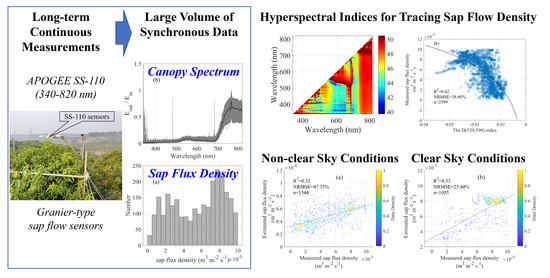
2.1. Research Site and Field Measurements

This study was conducted in an Integrated Remote Sensing Experimental Site for mango trees (23°42′09.5″N, 106°59′42.2″E, 151 m above sea level) located in the Baise National Agricultural Sci-tech Zone, Guangxi, China (see Figure 1a for the location). This region is characterized by a dry and hot valley with a prevalently subtropical monsoon climate. The annual mean temperature is estimated to be ca. 22 °C, but the extreme maximum temperature can reach 42 °C. The annual mean precipitation of this region is appropriately 1166 mm (mainly falling between May and September), while evaporation can reach approximately 1682 mm.
The experimental site, with a 10 m height observation tower, was established in 2018 to continuously monitor mango ecological processes, environmental factors, and hyperspectral remote sensing information. Canopy-scale water use was monitored through the Granier-type of thermal dissipation probes (12 mango trees in total) within a plot of the mango plantation. Environmental factors, including air temperature/humidity/pressure, wind speed/direction, precipitation, soil moisture/temperature, PAR, and net radiation, were also recorded. The incoming and outgoing radiations at 1 nm spectral resolution from 340 nm to 820 nm were monitored on a minute-scale after July 2019.
Synchronous measurements of canopy sap flux density and spectra were recorded from July 2019 to July 2021 at this site. The spectra were monitored with a pair of SS-110 field spectroradiometers (Apogee Instruments, Inc., USA), which can measure in-coming and out-going radiations at one nm interval over the wavelength domain from 340 to 820 nm. The spectroradiometers were mounted approximately 1 m above the mango tree in the vertical direction (Figure 1c). The upward-facing spectroradiometer was used to record the incoming solar radiation (energy flux density in W m−2 nm−1), while the downward-facing spectroradiometer was used to record the outgoing reflected radiation (energy flux density in W m−2 nm−1). The SS-110 field spectroradiometers were connected to a CR1000 (Campbell Scientific, Inc., Logan, UT, USA) data logger, in which the data were recorded every 1 min.
The Granier-type thermal dissipation probes (TDP) were installed on the trunks to monitor the sap flow of 12 mango trees (with diameters ranging from 14 to 26 cm). The sensors were sealed with silicone to protect from precipitation and were covered with waterproof foils to avoid thermal influences from radiation [1,33]. Four Granier sensors (in North, East, South, and West directions) were installed on the tree that was monitored with SS-110 sensors. All Grainer sensors were connected to a CR1000X (Campbell Scientific, Inc., USA) data logger, where data were recorded every 1 min and averaged every 10 min.

2.2. Data Preparations

2.2.1. Sap Flux Density

Sap flux density (Fd, m3 m−2 s−1) was calculated using the empirical equation given by Granier [34] and Lu et al. [35]:
F d = 118.99 × 10 6 ( Δ T m Δ T Δ T ) 1.231
where ΔTm is the temperature difference between the two probes at zero flux, and ΔT is the temperature difference between the heated and non-heated probes for positive xylem flow conditions.
As four Granier sensors in different directions were inserted into the tree trunk, the sap flux density was firstly calculated for each sensor and their averaged value was used for further analysis.

2.2.2. APOGEE-Based Canopy-Scale Reflectance

The canopy-scale reflectance was expressed with the ratio of outgoing radiation and incoming radiation measured with SS-110 field spectroradiometers at each specific wavelength. The calculated instantaneous spectra at the 1-min step were averaged for every 10 min in order to match the temporal resolution of sap flux density data. Hourly sap flux density was also generated similarly from the averaged values every 60 min for investigating the potential of hyperspectral indices to estimate water flux at a longer time scale.
As solar position (solar zenith and azimuth angles) has a great effect on in situ measurements of irradiation and reflectance [36,37] we, thus, calculated the sun position (zenith and azimuth angles at the site location) following the algorithm presented by Reda and Andreas [38] for each spectral measurement. Only data with the solar zenith angles less than 45° were used for further analysis.
Furthermore, we also introduced the clear sky index (Kt) to indicate the sky clearness at the moments of irradiation measurement [39]. The Kt was calculated with:
K t = I I e x t sin h
where I is the ground measured irradiance, Iext is extraterrestrial solar energy at the top of the atmosphere, and h is the solar elevation angle. As the SS-110 sensors only cover the wavelength region from 340 nm to 820 nm, and the sensitivity of the SS-110 is greater than 10% at wavelengths greater than 400 nm, we took the total irradiation (I) within 400–820 nm measured with the upward-facing SS-110 as ground observed energy density. The extraterrestrial solar energy density (Iext) within 400–820 nm was simulated from the LBLRTM (Line-By-Line Radiative Transfer Model, version 5.21) [40]. We defined the sky conditions as clear (Kt ≥ 0.4) or non-clear (cloudy or overcast, Kt < 0.4) based on the Kt [41,42].

2.2.3. Derivative Spectra

In addition to the calculated canopy-scale reflectance, the derivative spectra, which have been reported as effective in tracing leaf- and canopy-scale transpiration with different regression methods [1,43], were also calculated according to the “finite divided difference approximation” method [44,45]. The first-order derivative was expressed as:
d = d s d λ | i s ( λ i ) s ( λ j ) Δ λ
where s(λi) and s(λj) are the values of the spectrum (canopy reflectance here) at wavelength λi and λj, respectively, and Δλ is the wavelength increment between λi and λj. Higher-order derivatives were then calculated from lower-order derivatives iteratively. We analyzed low order (first to third) derivatives as derivatives (especially high orders) sensitive to noise [46].

2.3. Developing Hyperspectral Indices for Tracing Sap Flow Density

Based on the original reflectance and its derivative spectra, six commonly reported index types, including the given wavelength (R) with only one band; the simple ratio (SR), wavelength difference (D), a normalized difference (ND), and inverse differences (ID) with two spectral bands; the double differences (DDn), which involved three spectral bands, were used in this study for developing new indices [32]. The formula of these index types were presented in Table 1.
The raw spectra at the 1 nm spectral resolution were resampled to 5 nm with the five-point centered moving average method for shortening the time for index development. For all index types presented in Table 1, the index values for all possible combinations of the band(s) were first calculated from the spectra of each sample. A first-order polynomial linear regression was fit between the index values of the given combination of wavebands and the sap flux density values.

2.4. Statistical Criteria

The coefficient of determination (R2) was calculated for all indices and served as the primary statistical criteria for model selection:
R 2 = 1 - i n ( F d i F d ^ i ) 2 i n ( F d i F d ¯ ) 2
In addition to the coefficient of determination (R2), the ratio of performance to deviation (RPD) [47] and the normalized root mean square error by mean (NRMSE) was also calculated for each index as:
R P D = 1 n 1 i n ( F d i F d ¯ ) 2 1 n i n ( F d i F d ^ i ) 2
N R M S E = 1 n i n ( F d i F d ^ i ) 2 F d ¯ · Δ 100 %
where F d is the measured sap flux density value, F d ^ is the model fitted sap flux density value, F d ¯ is the mean sap flux density value for all samples, and n is the number of samples.

3. Results

3.1. Sap Flux Density and Canopy Reflected Spectra of Mango

A total of 2599 synchronous measurements (10-min) of sap flux density and spectra were selected (with solar zenith angles less than 45°) in this study. The mean value of sap flux density was 5.54 × 10⁻⁵ m3 m−2 s−1, with a standard deviation of 2.80 × 10⁻⁵ m3 m−2 s−1. Two distribution peaks around 2.25 × 10⁻⁵ m3 m−2 s−1 and 7.75 × 10⁻⁵ m3 m−2 s−1 can be recognized from Figure 2a. The synchronous measurements of canopy spectra were generated from incoming/outgoing radiations (energy flux density in W m−2 nm−1), shown in Figure 2b. The dashed line represents the mean values of all 2599 observations at each specific wavelength within the domain between 340 and 820 nm. The spectra at wavelengths between 340 and 380 nm were noisy because of the low sensitivity (<10%) of the SS-110 spectroradiometers within this spectral region.
The diurnal variations of sap flux density (10-min and hourly) under different sky conditions (clear, overcast, and cloudy) are illustrated in Figure 3. The maximum Kt values around noon on the 6, 7, and 8 of October 2019 were 0.52, 0.53, and 0.36, respectively. However, the mean Kt values from sunrise to sunset were 0.44, 0.36, and 0.23 on these three days. Under the clear sky conditions (the 6 October 2019), the sap flow increased quickly from sunrise and reached peak value around noon of the local solar time. Double peaks were observed under non-clear sky conditions (overcast or cloudy). Larger maximum Kt values also resulted in higher sap flux density peak values. The hourly sap flux density (dashed line) showed a time lag of approximately a half-hour if compared with the 10-min data series.

3.2. New Hyperspectral Indices for Tracking Sap Flux Density

Based on the 2599 synchronous data pairs, the best band combinations for each type of spectral index (listed in Table 1), calculated either from the original reflectance or transformed derivative spectra, were examined. The best index based on the original reflectance to trace the variation of sap flux density was the D-type index with the spectral bands of 520 nm and 590 nm. The D (520, 590) index could capture the change of canopy sap flux density with an R2 of 0.38 and an NRMSE of 39.69%. On the other hand, the best index identified based on the 1st order derivative spectra was the ND (475, 670) index, which had an R2 of 0.38 and an NRMSE of 39.82%, respectively. However, for higher-order derivatives (the 2nd and 3rd orders)-based indices, their performances decreased slightly. For instance, the R2 values of the D (415, 730), the best-performed index based on the 2nd order derivative, and the D (735, 790) index, the best one based on the 3rd order derivative spectra, were 0.29 and 0.30, respectively. Similarly, the R2 values of the ND-type of index based on the 2nd order and 3rd order derivatives decreased to 0.31 and 0.33, respectively. The diagram revealing the relationship between the field measured sap flux density and the D (520, 590) index is shown in Figure 4a. The fitting was improved when using a natural logarithmic function (R2 = 0.42).

3.3. Best Spectral Indices under Different Sky Conditions

We have further explored the performances of the spectral indices to trace the sap flux density under different sky conditions according to the clear sky index (Kt).
For cloudy/overcast sky conditions (Kt < 0.4), the bands 530 nm and 575 nm were identified as the best band combination for the D-, SR-, ND-, and ID-type of reflectance-based indices to trace the variation of sap flux density. Among them, the SR (530, 575), D (530, 575), ND (530, 575), and ID (530, 575) indices based on reflectance could trace the change of sap flux density with the R2 values of 0.31, 0.32, 0.32, and 0.28, respectively. The indices based on the derivative spectra were even poorer in estimating the sap flux density under non-clear sky conditions. The identified best indices based on the 1st, 2nd, and 3rd order derivatives were D (710, 735), ID (575, 650), and SR (735, 740). The R2 values of these three indices were only 0.26, 0.27, and 0.21, respectively. The relationship between field-measured sap flux density under non-clear sky conditions and the estimated values with the D (530, 575) index is shown in Figure 5a. The NRMSE and RPD values of the D (530, 575) index based on reflectance were 47.35% and 1.21 (n = 1544) for the sap flux density estimation under cloudy/overcast sky conditions.
On the other hand, for clear-sky conditions (Kt ≥ 0.4), much higher R2 values were achieved for all spectral forms (irrespective of original reflectance-based or derivatives-based). For all spectral forms, the best indices identified could trace the sap flux density with R2 values higher than 0.50. Among the six types of indices, the ID-type of index outperformed the other types of indices. Of the best indices identified, the ID (520, 560) index based on reflectance, the ID (410, 480) index based on the 1st order derivative, the ID (540, 575) index based on the 2nd order derivative, and the ID (555, 650) index based on the 3rd order derivative, could capture the variation of sap flux density under clear sky conditions with R2 values of 0.53 (NRMSE = 25.44%, RPD = 1.45), 0.50 (NRMSE = 26.12%, RPD = 1.42), 0.52 (NRMSE = 25.62%, RPD = 1.45), and 0.51 (NRMSE = 25.96%, RPD = 1.43), respectively. The scatter plot of the field measured sap flux density and estimated values with the ID (520, 560) index based on canopy reflectance is shown in Figure 5b. The results clearly indicate that the spectral indices were more effective in estimating sap flux density under clear sky conditions than those under non-clear sky conditions.

4. Discussion

4.1. Reported Indices vs. Newly Developed

Currently, there are already various narrow-band indices or multiple regression models (e.g., partial least squares regression) that have been developed from hyperspectral remotely sensed data for tracing plant transpiration [1,2,19,24,26,27,48,49,50]. Take hyperspectral indices as an example, Cao et al. [26] reported the exponential relationship between the SR (1580, 1600) index and canopy sap flow rate of Haloxylon ammodendron (R2 = 0.806). Marino et al. [24] and Sun et al. [49] suggested that the water index (WI) calculated with R900/R970 had good correlations with whole-plant (R2 = 0.668) and leaf-scale (R2 = 0.801) transpiration of Olea europaea L. Our previous research on Haloxylon ammodendron indicated that the simple ratio index dSR (660, 1040) based on the first-derivative spectra had an R2 of 0.54 with field measured canopy sap flow [1], and the normalized difference index ND (1425, 2145) had significant relationships (R2 = 0.40) with model-simulated and in situ measured canopy transpiration [27]. These reported results revealed the potential of hyperspectral narrow-band vegetation indices for fast, non-intrusive detection of plant transpiration. While we could not have evaluated these indices in this study because they used wavelengths beyond the covering range of SS-110 spectroradiometers, the Hyperspectral Normalized Difference Vegetation Index HNDVI (814, 672), proposed by Marshall et al. [19] showed a strong relationship with crop transpiration (R2 = 0.68) and has been evaluated explicitly. Validation results showed that the index had a very poor performance with the measured sap flows of mango trees, with an R2 value of 0.005 only (NRMSE = 50.37% and RPD = 1.00). The sensitivity of spectral indices was species-dependent [51] and may be the primary reason for this discrepancy.
The newly developed hyperspectral indices in this study, together with several reported hyperspectral narrow-band indices, provided a new way to monitor water flux directly and non-intrusively. However, addressing the underlying mechanisms remains a great challenge. The critical role of stomatal conductance (gs) in regulating plant water use has been clarified [52], with its short-term changes linked closely to the hydraulic properties to minimize the loss of hydraulic conductivity through xylem [53]. Remote estimation of stomatal conductance with normalized difference vegetation indices was reported in the 1990s, and the results showed strong linear or non-linear relationships between gs and vegetation indices [54,55,56]. Further recent research on hyperspectral remote sensing of stomatal conductance revealed that the indices with the yellow (570–630 nm) and green (530–580 nm) spectral region were highly correlated with gs [57]. The importance of the yellow band in gs estimation was also confirmed with partial least squares regression analysis [57]. In addition, the bands 530 nm, 550 nm, and 580 nm have also been selected as important spectral features using stepwise regression analysis for the remote sensing of gs [58]. Consequently, the bands used in the newly developed hyperspectral indices in this study (520, 530, 560, 575, and 590 nm) for water use estimation agree well with the reported spectral region of stomatal conductance, revealing the underlying physiological mechanisms to a certain level. Although these spectral bands have not been directly linked to plant water use, the photochemical reflectance index (PRI), or some modified PRIs involved these bands, were strongly correlated with photosynthetic parameters which can be caused by changes in stomata-opening [59]. The PRI has been reported as a useful tool for the remote sensing of plant water stress at the canopy level [60].

4.2. Effects of Spectral Transformations

Derivative analysis has been reported as feasible for estimating plant biophysical and biochemical parameters as it holds the advantages of minimizing additive constants and linear functions [46]. Many derivative spectra-based indices have been reported to be more effective than reflectance-based indices for deriving biophysical and biochemical quantities [1,30,61,62,63]. Several pieces of research on hyperspectral remote sensing of water flux also indicated that the derivative spectra performed better in estimating the variations in leaf transpiration [43] or canopy transpiration [1].
In this study, we investigated the performances of hyperspectral indices based on reflectance as well as derivatives to estimate canopy-scale sap flux density. Unlike the results reported by Wang and Jin [43] and Jin and Wang [1], where derivative spectra showed better accuracies in tracking leaf transpiration using partial least squares regression (PLSR) [43] and quantifying canopy sap flux density with hyperspectral indices [1], the best hyperspectral indices identified in this study were those based on reflectance rather than those based on derivative spectra. The limit wavelength range of the SS-100 spectroradiometer may have possibly confined those better combinations using longer wavelengths for derivative indices and might explain the discrepancy. However, this result was consistent with our previous research on canopy transpiration estimation with hyperspectral indices in a simulated database (n = 2204) with The Soil Canopy Observation of Photosynthesis and Energy fluxes (SCOPE) model [27], where the first-order derivative spectra-based indices were tested but they did not result in significant improvement to estimate transpiration in the simulated dataset with large sample numbers.
To compare the performance of reflectance and derivative spectra to estimate sap flux density, we illustrated the correlation coefficients of the measured sap flux density and the spectra (reflectance and the 1st derivative spectra) at each wavelength in Figure 6. The correlation coefficients between sap flux density and the 1st order derivative spectra were all between −0.1 and 0.1 throughout the wavelength from 400 nm to 820 nm, while the reflectance values around 500 nm and 670 nm were relatively significant (correlation coefficients around 0.16) and correlated with sap flux density. Furthermore, the reflectance around 570 nm was insensitive (correlation coefficients around 0) to sap flux density, and the bands around here were involved in many indices presented in Section 3.

4.3. Performances of Developed Hyperspectral Indices at Different Time-Scales

The dynamic processes of sap flow and the environmental factors are not entirely synchronous due to the time lag between them [64]. A direct comparison between measurements of sap flow and transpiration within a clear day suggested that sap flow lagged behind transpiration (a 1 h time lag gave the best fit between the sap flow and transpiration) [65]. Our results illustrated in Figure 3 also showed that the sap flow averaged to every 60 min lagged approximately a half-hour behind the 10-min averaged values. To discuss the potential of hyperspectral indices to estimate water flux over a longer time scale, we have further examined their relationship on an hourly-scale.
The results (shown in Figure 7) were similar to those generated based on 10-min averaged data. The hyperspectral indices developed from reflectance could trace hourly sap flux density with an R2 value of 0.36 under all-sky conditions (n = 352), 0.32 under cloudy or overcast sky conditions (n = 223), and 0.57 under clear sky conditions, respectively. These findings highlight a promising strategy for developing hyperspectral indices to potentially characterize water flux on broad-scales.
Notably, the remotely sensed data and field survey are responsible for the model accuracy in plant biophysical parameter prediction [66,67,68]. Seasonal variation of PRI and Tc-Ta (the difference between crown temperature and air temperature) also demonstrated a time delay of PRI for water stress (stomatal conductance and water potential) detection [69]. Thus, we realized that the time lag effect in the sensitivity of hyperspectral indices for sap flux density estimation should be taken into account in future studies.

4.4. Pros and Cons of Proximally Sensed Reflected Spectra on Investigating Canopy Functions

Hyperspectral remote sensing is a rapid, non-invasive, and efficient technique for monitoring the biochemical or biophysical status of vegetation [70]. Compared with the traditional field measurements of plant water use, proximal remote sensing has great potential for monitoring real-time plant water use non-invasively. However, unlike the well-examined biophysical and biochemical parameters, the underlying fundamental mechanisms for the remote sensing of plant functions (such as photosynthesis-related parameters, transpiration rate, etc.) are still unclear. For short periods, the physiological status of vegetation, including water and carbon fluxes, are controlled in part by considerably changing stomatal resistance [52]. However, over longer periods (weeks or months), plants tend to adjust their foliage density to match the capacity of the environment to support photosynthesis [71]. Hence, the time-series of vegetation indices should be further explored when using remotely-sensed instantaneous data to measure the physiological status of vegetation. Moreover, the background noise and interference is also an issue when directly scaling carbon and water fluxes using canopy spectral signals [44]. Different analysis approaches should also be involved to improve the estimation precession of transpiration or other plant function parameters from time-series remote sensing data.

5. Conclusions

Based on the continuously field-monitored minute-scale canopy reflected spectra and sap flow, we verified the feasibility of using narrow-band indices based on reflectance as well as derivatives to trace canopy-scale water use (sap flux density) in this study. Although the D (520, 590) index calculated from canopy reflectance had an overall R2 of 0.38, an index that performed much better, ID (520, 560), was developed to track canopy water use under clear sky conditions (clear sky index ≥ 0.4). The bands used in these indices agreed well with the reported sensitive wavelengths regarding stomatal conductance, partially revealing their underlying physiological mechanisms. The results obtained in this study should provide valuable insights for non-invasively retrieving canopy transpiration from proximal remotely sensed data.

Author Contributions

J.J. designed this study; J.J. carried out the analyses; N.H., Y.H., Y.Y., X.Z. and M.W. collected field data and managed the database; J.J. wrote the manuscript; all authors reviewed the manuscript. All authors have read and agreed to the published version of the manuscript.

Funding

This research was supported by the National Natural Science Foundation of China (No. 41901368) and the Guangxi Science and Technology Projects (Guike AD21220085, Guike AD20238059).

Institutional Review Board Statement

Not applicable.

Informed Consent Statement

Not applicable.

Data Availability Statement

The data that support the findings of this study are available on request from the corresponding author.

Acknowledgments

We thank the members of the International Joint Laboratory of Ecology and Remote Sensing, Nanning Normal University, for their support of the fieldwork.

Conflicts of Interest

The authors declare no conflict of interest.

References

  1. Jin, J.; Wang, Q. Hyperspectral indices based on first derivative spectra closely trace canopy transpiration in a desert plant. Ecol. Inform. 2016, 35, 1–8. [Google Scholar] [CrossRef]
  2. Weksler, S.; Rozenstein, O.; Haish, N.; Moshelion, M.; Wallach, R.; Ben-Dor, E. Detection of Potassium Deficiency and Momentary Transpiration Rate Estimation at Early Growth Stages Using Proximal Hyperspectral Imaging and Extreme Gradient Boosting. Sensors 2021, 21, 958. [Google Scholar] [CrossRef]
  3. McDowell, N.G.; White, S.; Pockman, W.T. Transpiration and stomatal conductance across a steep climate gradient in the southern Rocky Mountains. Ecohydrology 2008, 1, 193–204. [Google Scholar] [CrossRef] [Green Version]
  4. Nordey, T.; Lechaudel, M.; Saudreau, M.; Joas, J.; Genard, M. Model-assisted analysis of spatial and temporal variations in fruit temperature and transpiration highlighting the role of fruit development. PLoS ONE 2014, 9, e92532. [Google Scholar] [CrossRef] [Green Version]
  5. Steppe, K.; De Pauw, D.J.W.; Doody, T.M.; Teskey, R.O. A comparison of sap flux density using thermal dissipation, heat pulse velocity and heat field deformation methods. Agric. For. Meteorol. 2010, 150, 1046–1056. [Google Scholar] [CrossRef]
  6. Granier, A.; Biron, P.; Lemoine, D. Water balance, transpiration and canopy conductance in two beech stands. Agric. For. Meteorol. 2000, 100, 291–308. [Google Scholar] [CrossRef]
  7. Verstraeten, W.W.; Veroustraete, F.; Feyen, J. Assessment of Evapotranspiration and Soil Moisture Content Across Different Scales of Observation. Sensors 2008, 8, 70–117. [Google Scholar] [CrossRef] [PubMed] [Green Version]
  8. Fisher, J.B.; Lee, B.; Purdy, A.J.; Halverson, G.H.; Dohlen, M.B.; Cawse-Nicholson, K.; Wang, A.; Anderson, R.G.; Aragon, B.; Arain, M.A.; et al. ECOSTRESS: NASA’s next generation mission to measure evapotranspiration from the International Space Station. Water Resour. Res. 2020, 56, e2019WR026058. [Google Scholar] [CrossRef]
  9. Gogoi, N.; Deka, B.; Bora, L. Remote sensing and its use in detection and monitoring plant diseases: A review. Agric. Rev. 2018, 39, 307–313. [Google Scholar] [CrossRef]
  10. Glenn, E.P.; Nagler, P.L.; Huete, A.R. Vegetation Index Methods for Estimating Evapotranspiration by Remote Sensing. Surv. Geophys. 2010, 31, 531–555. [Google Scholar] [CrossRef]
  11. Wang, K.; Dickinson, R.E. A review of global terrestrial evapotranspiration: Observation, modeling, climatology, and climatic variability. Rev. Geophys. 2012, 50, RG2005. [Google Scholar] [CrossRef]
  12. Courault, D.; Seguin, B.; Olioso, A. Review on estimation of evapotranspiration from remote sensing data: From empirical to numerical modeling approaches. Irrig. Drain. Syst. 2005, 19, 223–249. [Google Scholar] [CrossRef]
  13. Boegh, E.; Soegaard, H.; Hanan, N.; Kabat, P.; Lesch, L. A Remote Sensing Study of the NDVI–Ts Relationship and the Transpiration from Sparse Vegetation in the Sahel Based on High-Resolution Satellite Data. Remote Sens. Environ. 1999, 69, 224–240. [Google Scholar] [CrossRef]
  14. Su, Z. The Surface Energy Balance System (SEBS) for estimation of turbulent heat fluxes. Hydrol. Earth Syst. Sci. 2002, 6, 85–100. [Google Scholar] [CrossRef]
  15. Allen, R.G.; Tasumi, M.; Trezza, R. Satellite-based energy balance for mapping evapotranspiration with internalized calibration (METRIC)—Model. J. Irrig. Drain. Eng. 2007, 133, 380–394. [Google Scholar] [CrossRef]
  16. Bastiaanssen, W.G.M.; Menenti, M.; Feddes, R.A.; Holtslag, A.A.M. A remote sensing surface energy balance algorithm for land (SEBAL). 1. Formulation. J. Hydrol. 1998, 212–213, 198–212. [Google Scholar] [CrossRef]
  17. Page, G.F.M.; Liénard, J.F.; Pruett, M.J.; Moffett, K.B. Spatiotemporal dynamics of leaf transpiration quantified with time-series thermal imaging. Agric. For. Meteorol. 2018, 256-257, 304–314. [Google Scholar] [CrossRef]
  18. Gowda, P.H.; Chavez, J.L.; Colaizzi, P.D.; Evett, S.R.; Howell, T.A.; Tolk, J.A. ET mapping for agricultural water management: Present status and challenges. Irrig. Sci. 2008, 26, 223–237. [Google Scholar] [CrossRef] [Green Version]
  19. Marshall, M.; Thenkabail, P.; Biggs, T.; Post, K. Hyperspectral narrowband and multispectral broadband indices for remote sensing of crop evapotranspiration and its components (transpiration and soil evaporation). Agric. For. Meteorol. 2016, 218–219, 122–134. [Google Scholar] [CrossRef] [Green Version]
  20. Jasechko, S.; Sharp, Z.D.; Gibson, J.J.; Birks, S.J.; Yi, Y.; Fawcett, P.J. Terrestrial water fluxes dominated by transpiration. Nature 2013, 496, 347–350. [Google Scholar] [CrossRef]
  21. Glenn, E.P.; Huete, A.R.; Nagler, P.L.; Hirschboeck, K.K.; Brown, P. Integrating Remote Sensing and Ground Methods to Estimate Evapotranspiration. Crit. Rev. Plant Sci. 2007, 26, 139–168. [Google Scholar] [CrossRef]
  22. Kato, T.; Kimura, R.; Kamichika, M. Estimation of evapotranspiration, transpiration ratio and water-use efficiency from a sparse canopy using a compartment model. Agric. Water Manag. 2004, 65, 173–191. [Google Scholar] [CrossRef]
  23. Reynolds, J.F.; Kemp, P.R.; Tenhunen, J.D. Effects of long-term rainfall variability on evapotranspiration and soil water distribution in the Chihuahuan Desert: A modeling analysis. Plant Ecol. 2000, 150, 145–159. [Google Scholar] [CrossRef]
  24. Marino, G.; Pallozzi, E.; Cocozza, C.; Tognetti, R.; Giovannelli, A.; Cantini, C.; Centritto, M. Assessing gas exchange, sap flow and water relations using tree canopy spectral reflectance indices in irrigated and rainfed Olea europaea L. Environ. Exp. Bot. 2014, 99, 43–52. [Google Scholar] [CrossRef]
  25. El-Hendawy, S.; Al-Suhaibani, N.; Hassan, W.; Tahir, M.; Schmidhalter, U. Hyperspectral reflectance sensing to assess the growth and photosynthetic properties of wheat cultivars exposed to different irrigation rates in an irrigated arid region. PLoS ONE 2017, 12, e0183262. [Google Scholar] [CrossRef]
  26. Cao, X.; Wang, J.; Chen, X.; Gao, Z.; Yang, F.; Shi, J. Multiscale remote-sensing retrieval in the evapotranspiration of Haloxylon ammodendron in the Gurbantunggut desert, China. Environ. Earth Sci. 2013, 69, 1549–1558. [Google Scholar] [CrossRef]
  27. Jin, J.; Wang, Q.; Wang, J. Combing both simulated and field-measured data to develop robust hyperspectral indices for tracing canopy transpiration in drought-tolerant plant. Environ. Monit. Assess. 2019, 191, 13. [Google Scholar] [CrossRef]
  28. le Maire, G.; François, C.; Soudani, K.; Berveiller, D.; Pontailler, J.-Y.; Bréda, N.; Genet, H.; Davi, H.; Dufrêne, E. Calibration and validation of hyperspectral indices for the estimation of broadleaved forest leaf chlorophyll content, leaf mass per area, leaf area index and leaf canopy biomass. Remote Sens. Environ. 2008, 112, 3846–3864. [Google Scholar] [CrossRef]
  29. Rady, A.M.; Guyer, D.E.; Kirk, W.; Donis-González, I.R. The potential use of visible/near infrared spectroscopy and hyperspectral imaging to predict processing-related constituents of potatoes. J. Food Eng. 2014, 135, 11–25. [Google Scholar] [CrossRef]
  30. Imanishi, J.; Sugimoto, K.; Morimoto, Y. Detecting drought status and LAI of two Quercus species canopies using derivative spectra. Comput. Electron. Agric. 2004, 43, 109–129. [Google Scholar] [CrossRef]
  31. Jin, J.; Wang, Q.; Song, G. Selecting informative bands for partial least squares regressions improves their goodness-of-fits to estimate leaf photosynthetic parameters from hyperspectral data. Photosynth. Res. 2021, 151, 71–82. [Google Scholar] [CrossRef] [PubMed]
  32. Jin, J.; Arief Pratama, B.; Wang, Q. Tracing Leaf Photosynthetic Parameters Using Hyperspectral Indices in an Alpine Deciduous Forest. Remote Sens. 2020, 12, 1124. [Google Scholar] [CrossRef] [Green Version]
  33. Zheng, C.; Wang, Q. Water-use response to climate factors at whole tree and branch scale for a dominant desert species in central Asia: Haloxylon ammodendron. Ecohydrology 2014, 7, 56–63. [Google Scholar] [CrossRef]
  34. Granier, A. A new method of sap flow measurement in tree stems. Ann. Sci. For. 1985, 42, 193–200. [Google Scholar] [CrossRef]
  35. Lu, P.; Urban, L.; Zhao, P. Granier’s thermal dissipation probe (TDP) method for measuring sap flow in trees: Theory and practice. Acta Bot. Sin. 2004, 46, 631–646. [Google Scholar]
  36. Blanc, P.; Wald, L. On the effective solar zenith and azimuth angles to use with measurements of hourly irradiation. Adv. Sci. Res. 2016, 13, 1–6. [Google Scholar] [CrossRef] [Green Version]
  37. Shibayama, M.; Wiegand, C.L. View azimuth and zenith, and solar angle effects on wheat canopy reflectance. Remote Sens. Environ. 1985, 18, 91–103. [Google Scholar] [CrossRef]
  38. Reda, I.; Andreas, A. Solar position algorithm for solar radiation applications. Solar Energy 2004, 76, 577–589. [Google Scholar] [CrossRef]
  39. Liu, B.Y.H.; Jordan, R.C. The interrelationship and characteristic distribution of direct, diffuse and total solar radiation. Solar Energy 1960, 4, 1–19. [Google Scholar] [CrossRef]
  40. Clough, S.; Brown, P.; Liljegren, J.; Shippert, T.; Turner, D.; Knuteson, R.; Revercomb, H.; Smith, W. Implications for atmospheric state specification from the AERI/LBLRTM quality measurement experiment and the MWR/LBLRTM quality measurement experiment. In Proceedings of the 6th ARM Science Team Meeting, San Antonio, TX, USA, 4–7 March 1996. [Google Scholar]
  41. Hu, B.; Wang, Y.; Liu, G. Influences of the clearness index on UV solar radiation for two locations in the Tibetan Plateau-Lhasa and Haibei. Adv. Atmos. Sci. 2008, 25, 885–896. [Google Scholar] [CrossRef]
  42. Cañada, J.; Pedrós, G.; López, A.; Boscá, J.V. Influences of the clearness index for the whole spectrum and of the relative optical air mass on UV solar irradiance for two locations in the Mediterranean area, Valencia and Cordoba. J. Geophys. Res. Atmos. 2000, 105, 4759–4766. [Google Scholar] [CrossRef]
  43. Wang, Q.; Jin, J. Leaf transpiration of drought tolerant plant can be captured by hyperspectral reflectance using PLSR analysis. iForest—Biogeosciences For. 2015, 9, 30–37. [Google Scholar] [CrossRef] [Green Version]
  44. Tsai, F.; Philpot, W. Derivative Analysis of Hyperspectral Data. Remote Sens. Environ. 1998, 66, 41–51. [Google Scholar] [CrossRef]
  45. Chapra, S.C.; Canale, R.P. Numerical Methods for Engineers; McGraw-Hill: New York, NY, USA, 1988; Volume 2. [Google Scholar]
  46. Wang, Q.; Jin, J.; Sonobe, R.; Chen, J.M. Derivative hyperspectral vegetation indices in characterizing forest biophysical and biochemical quantities. In Hyperspectral Indices and Image Classifications for Agriculture and Vegetation; Thenkabail, P.S., Lyon, J.G., Huete, A., Eds.; CRC Press: Boca Raton, FL, USA, 2018; pp. 27–63. [Google Scholar] [CrossRef]
  47. Williams, P.C. Variable affecting near infrared reflectance spectroscopic analysis. In Near-Infrared Technology in the Agriculture and Food Industries; Williams, P., Norris, K., Eds.; American Association of Cereal Chemists Inc.: Saint Paul, MN, USA, 1987; pp. 143–167. [Google Scholar]
  48. El-Hendawy, S.; Al-Suhaibani, N.; Alotaibi, M.; Hassan, W.; Elsayed, S.; Tahir, M.U.; Mohamed, A.I.; Schmidhalter, U. Estimating growth and photosynthetic properties of wheat grown in simulated saline field conditions using hyperspectral reflectance sensing and multivariate analysis. Sci. Rep. 2019, 9, 16473. [Google Scholar] [CrossRef]
  49. Sun, P.; Wahbi, S.; Tsonev, T.; Haworth, M.; Liu, S.; Centritto, M. On the Use of Leaf Spectral Indices to Assess Water Status and Photosynthetic Limitations in Olea europaea L. during Water-Stress and Recovery. PLoS ONE 2014, 9, e105165. [Google Scholar] [CrossRef] [Green Version]
  50. Zhou, J.-J.; Zhang, Y.-H.; Han, Z.-M.; Liu, X.-Y.; Jian, Y.-F.; Hu, C.-G.; Dian, Y.-Y. Hyperspectral sensing of photosynthesis, stomatal conductance, and transpiration for citrus tree under drought condition. bioRxiv 2021. [Google Scholar] [CrossRef]
  51. Eitel, J.U.H.; Gessler, P.E.; Smith, A.M.S.; Robberecht, R. Suitability of existing and novel spectral indices to remotely detect water stress in Populus spp. For. Ecol. Manag. 2006, 229, 170–182. [Google Scholar] [CrossRef]
  52. Collatz, G.J.; Ball, J.T.; Grivet, C.; Berry, J.A. Physiological and environmental regulation of stomatal conductance, photosynthesis and transpiration: A model that includes a laminar boundary layer. Agric. For. Meteorol. 1991, 54, 107–136. [Google Scholar] [CrossRef]
  53. Whitehead, D. Regulation of stomatal conductance and transpiration in forest canopies. Tree Physiol. 1998, 18, 633–644. [Google Scholar] [CrossRef]
  54. Carter, G.A. Reflectance Wavebands and Indices for Remote Estimation of Photosynthesis and Stomatal Conductance in Pine Canopies. Remote Sens. Environ. 1998, 63, 61–72. [Google Scholar] [CrossRef]
  55. Verma, S.B.; Sellers, P.J.; Walthall, C.L.; Hall, F.G.; Kim, J.; Goetz, S.J. Photosynthesis and stomatal conductance related to reflectance on the canopy scale. Remote Sens. Environ. 1993, 44, 103–116. [Google Scholar] [CrossRef]
  56. Myneni, R.B.; Ganapol, B.D.; Asrar, G. Remote sensing of vegetation canopy photosynthetic and stomatal conductance efficiencies. Remote Sens. Environ. 1992, 42, 217–238. [Google Scholar] [CrossRef]
  57. Maimaitiyiming, M.; Ghulam, A.; Bozzolo, A.; Wilkins, J.L.; Kwasniewski, M.T. Early Detection of Plant Physiological Responses to Different Levels of Water Stress Using Reflectance Spectroscopy. Remote Sens. 2017, 9, 745. [Google Scholar] [CrossRef] [Green Version]
  58. Jarolmasjed, S.; Sankaran, S.; Kalcsits, L.; Khot, L.R. Proximal hyperspectral sensing of stomatal conductance to monitor the efficacy of exogenous abscisic acid applications in apple trees. Crop Protect. 2018, 109, 42–50. [Google Scholar] [CrossRef]
  59. Sukhova, E.; Sukhov, V. Relation of Photochemical Reflectance Indices Based on Different Wavelengths to the Parameters of Light Reactions in Photosystems I and II in Pea Plants. Remote Sens. 2020, 12, 1312. [Google Scholar] [CrossRef] [Green Version]
  60. Evain, S.; Flexas, J.; Moya, I. A new instrument for passive remote sensing: 2. Measurement of leaf and canopy reflectance changes at 531 nm and their relationship with photosynthesis and chlorophyll fluorescence. Remote Sens. Environ. 2004, 91, 175–185. [Google Scholar] [CrossRef]
  61. Yao, X.; Ren, H.; Cao, Z.; Tian, Y.; Cao, W.; Zhu, Y.; Cheng, T. Detecting leaf nitrogen content in wheat with canopy hyperspectrum under different soil backgrounds. Int. J. Appl. Earth Obs. Geoinf. 2014, 32, 114–124. [Google Scholar] [CrossRef]
  62. Demetriades-Shah, T.H.; Steven, M.D.; Clark, J.A. High resolution derivative spectra in remote sensing. Remote Sens. Environ. 1990, 33, 55–64. [Google Scholar] [CrossRef]
  63. Zarco-Tejada, P.J.; Pushnik, J.C.; Dobrowski, S.; Ustin, S.L. Steady-state chlorophyll a fluorescence detection from canopy derivative reflectance and double-peak red-edge effects. Remote Sens. Environ. 2003, 84, 283–294. [Google Scholar] [CrossRef]
  64. Tu, J.; Wei, X.; Huang, B.; Fan, H.; Jian, M.; Li, W. Improvement of sap flow estimation by including phenological index and time-lag effect in back-propagation neural network models. Agric. For. Meteorol. 2019, 276–277, 107608. [Google Scholar] [CrossRef]
  65. Saugier, B.; Granier, A.; Pontailler, J.Y.; Dufrêne, E.; Baldocchi, D.D. Transpiration of a boreal pine forest measured by branch bag, sap flow and micrometeorological methods. Tree Physiol. 1997, 17, 511–519. [Google Scholar] [CrossRef] [PubMed]
  66. Haagsma, M.; Page, G.F.M.; Johnson, J.S.; Still, C.; Waring, K.M.; Sniezko, R.A.; Selker, J.S. Model selection and timing of acquisition date impacts classification accuracy: A case study using hyperspectral imaging to detect white pine blister rust over time. Comput. Electron. Agric. 2021, 191. [Google Scholar] [CrossRef]
  67. Darmawan, A.; Nadirah, A.W.; Evri, M.; Mulyono, S.; Nugroho, A.; Sadly, M.; Hendiarti, N.; Kashimura, O.; Kobayashi, C.; Uchida, A. Quantitative analysis from unifying field and airborne hyperspectral in prediction biophysical parameters by using partial least square (PLSR) and Normalized Difference Spectral Index (NDSI). In Proceedings of the 30th Asian Conference on Remote Sensing (ACRS), Beijing, China, 18–23 October 2009. TS10-02. [Google Scholar]
  68. Yang, C.; Everitt, J.H.; Bradford, J.M. Yield Estimation from Hyperspectral Imagery Using Spectral Angle Mapper (SAM). Trans. ASABE 2008, 51, 729–737. [Google Scholar] [CrossRef]
  69. Zarco-Tejada, P.J.; González-Dugo, V.; Berni, J.A.J. Fluorescence, temperature and narrow-band indices acquired from a UAV platform for water stress detection using a micro-hyperspectral imager and a thermal camera. Remote Sens. Environ. 2012, 117, 322–337. [Google Scholar] [CrossRef]
  70. Thenkabail, P.S.; Lyon, J.G.; Huete, A. Hyperspectral Remote Sensing of Vegetation; CRC Press: Boca Raton, FL, USA, 2012. [Google Scholar]
  71. Glenn, E.P.; Huete, A.R.; Nagler, P.L.; Nelson, S.G. Relationship between remotely-sensed vegetation indices, canopy attributes and plant physiological processes: What vegetation indices can and cannot tell us about the landscape. Sensors 2008, 8, 2136–2160. [Google Scholar] [CrossRef] [Green Version]
Figure 1. Research site location (a), an overview of the plot (b), and the setting of SS-110 spectrometers over the canopy (c).
Remotesensing 14 01483 g001
Figure 2. Variations of field-measured sap flux density (a) and spectra in 5 nm resolution (b).
Remotesensing 14 01483 g002
Figure 3. Diurnal variations of sap flux density under different sky conditions. (a) clear, (b) cloudy, (c) overcast.
Remotesensing 14 01483 g003
Figure 4. The relationship between the D (520, 590) index based on reflectance and the measured sap flux density with Grainer sensors. The black dashed line is the regression line (a) fitted with a polynomial regression (linear to the first order), (b) fitted with a natural logarithmic function.
Remotesensing 14 01483 g004
Figure 5. Scatter plots of the measured sap flux density and the estimated values with the spectral indices based on reflectance. (a) The D (530, 575) index for non-clear sky conditions, (b) the ID (520, 560) index for clear sky conditions.
Remotesensing 14 01483 g005
Figure 6. Correlation test between sap flux density and spectra (reflectance and the 1st order derivative spectra) at each wavelength.
Remotesensing 14 01483 g006
Figure 7. Relationships between the best indices identified and sap flux density (averaged to every 60 min) estimations under different sky conditions. (a) All-sky conditions, (b) cloudy or overcast sky conditions, (c) clear sky conditions.
Remotesensing 14 01483 g007
Table 1. The formula of different index types used in this study.
Index TypeFormula of IndexNumber of Bands
1.R(λ) = S λ *1
2.SR(λ1, λ2) = S λ 1 S λ 2 2
3.D(λ1, λ2) = S λ 1 S λ 2 2
4.ND(λ1, λ2) = ( S λ 1 S λ 2 ) ( S λ 1 + S λ 2 ) 2
5.ID(λ1, λ2) = 1 S λ 1 1 S λ 2 2
6.DDn(λ1, Δλ) = 2 S λ 1 S λ 1 Δ λ S λ 1 + Δ λ 3
* Sλ is the spectrum value (reflectance or derivative) at the specific wavelength λ.
Publisher’s Note: MDPI stays neutral with regard to jurisdictional claims in published maps and institutional affiliations.

