1. Introduction
The best choice of a digital model of a given terrain is a significant element in model studies of agricultural watersheds. It has a significant impact on the precision of mapping of boundaries of a watershed and the watercourses occurring there. Numerous studies concerning the selection of the precision and source of a DEM have been carried out; these have been performed using data from the Shuttle Radar Topography Mission, the Aster scanner of the Terra satellite, or LiDAR measurements, or data generated based on topography maps or terrain measurements [
1,
2,
3,
4,
5,
6,
7]. The impact of various methods—in performance, processing, and introduction of corrections—on the precision of DEMs and their usefulness for hydrological modeling have also been extensively investigated [
8,
9,
10,
11,
12]. These studies often aimed to investigate these data sources and explore which methods of preparation would enable the most precise results of modeling to be obtained.
Presently, measuring techniques are well-developed, and the cost of obtaining data has significantly decreased. Therefore, frequently, the aim of the studies is to refine the speed of DEM analyses and the delineation of watercourses and watershed boundaries—without necessarily focusing on obtaining the highest possible precision. New algorithms for determining the course of the boundaries of a watershed have been created based on the maps of gradients of the terrain determined with a DEM; additional developments include the following: [
13] proposes new programs for the automatization of manual operations which are currently performed for the delineation of watercourses and boundaries of a watershed [
14]; alternative methods—which are simple for computing—for determining the borders of a watershed based on the course of watercourses are tested in [
15]. However, the most numerous in the literature are studies where, in order to speed up the creation of a model, the frequency of an original DEM is reduced, and the impact of this operation on the precision of the obtained results is verified. DEMs from various sources and of varied resolutions, were analyzed in the following: DEMs with resolutions of 1–2 m were made based on the data from LiDAR measurements [
1,
16,
17,
18,
19], those of 5–10 m were made based on topographical maps [
20,
21,
22], and those of 30–90 m were made based on satellite measurements [
5,
16]. In all cases, it was necessary for the researchers to make a decision concerning the resolution-change method. The justification of these choices was either noticeably short, or there was no justification at all. Moreover, in the above studies, no attempt was made to verify the effects of the chosen resolution-change methods. This issue was undertaken by, inter alia, Arun [
8], Goyal et al. [
4], Haile and Rientjes [
23], Dixon and Earls [
2], Tan et al. [
24], Coz et al. [
25], and Wu et al. [
26]. To reduce the resolution, most often, they used tools for interpolation with nearest neighbor methods, bilinear interpolation, or bicubic convolution. Only Coz et al. [
25] used statistical methods of aggregation, namely giving higher pixels an average, modal, medial, minimum, or maximum values.
No studies were found on the impact of statistical methods of DEM aggregation, in particular LiDAR ones, on the usefulness of DEMs for hydrological modeling and, in particular, on its initial stage—namely on the delineation of watercourses and boundaries of a watershed and computing their parameters, such as the length and gradient of watercourses.
Li and Wong [
16] studied the change in DEM resolution to use it for the delineation of watersheds and watercourses, based on the conclusions made by Haile and Rientjes [
23], who researched the impact of various methods of resolution change on the modeling of the flood range, in particular in developed areas, and examined the change in resolution with the use of the interpolation nearest neighbor method, bilinear interpolation, and the bicubic method from 1.5 m to 10 m. Li and Wong used the interference from this study, since there are no such conclusions on the impact of the DEM resampling method on its use for the delineation of the watercourses and boundaries of a watershed. In the current study, the impact of a DEM on the delineation of the watershed boundaries was assessed based on the watershed size [
27]. When the size of a pixel is changed, the reduction in the area of one watershed must be compensated with the increase in the area of another one, and when a higher number of watersheds is analyzed, the change in their sizes will approach zero.
There is no analysis of the correctness of the locations of the watershed boundaries; thus, in the present study, the precision of the delineation of the boundaries of a watershed in the SWAT model interface [
28] (QSWAT [
29]) was assessed, not only the size of its area.
2. Materials and Methods
A watershed of the Zgłowiączka River headwaters—with the area of 90 km
2, located in the Kujawsko-Pomorskie voivodeship, between the latitudes of 52°34′50′′–52°41′15′′N and the longitudes of 18°33′24′′–18°46′12′′E—was the investigated area. The superficial layer consists of quaternary clays in almost the entire area. Their thickness is from 25 to 90 m. The surface area of the watershed of the Zgłowiączka River is very flat. The difference in between the highest and the lowest point is only 44 m. Very fertile phaeozems with a small share of podzolic soil prevail on the entire area of the watershed. The Zgłowiączka River is a left, primary tributary of the Vistula River. The average gradient of the riverbed is 0.6%, and the average flow during the years 1961–2000 from the estuary to the Vistula River on the post in Włocławek Ruda was 3.95 m
3·s
−1 [
30]. The watershed of the Zgłowiączka River, like the majority of Poland, lies in the warm region, with the sum of average daily temperatures ≥10 °C within 2750–3000 °C a year. With regard to precipitation, this area is exceptionally dry, with a precipitation index at the level of 50 [
31,
32,
33]. Although, precipitation in the area of the Zgłowiączka River is extremely low, high-quality soil obtains a high yield; thus, agriculture is very intense and covers almost the entire area of the watershed.
The Zgłowiączka River watershed has been previously modelled in order to support the implementation of the Framework Water Directive in Poland [
34], the determination of the dislocation ways and the size of the nitrogen loads [
35], and the influence of permanent grasslands on nitrogen loads [
36]. The considerable anthropogenic transformation of the natural hydrological conditions of the Zgłowiączka River watershed has caused many problems [
35].
2.1. Source DEM and Its Aggregation
A DEM with 1 m resolution and an average error of height up to 0.2 m, created based on air LiDAR measurements made available by the Head Office of Geodesy and Cartography, was applied in the study. The accuracy was estimated by the geodetic measurements [
37]. Subsequent values of resolution of the investigated DEM were obtained by an increase by a half of the previous resolution values, starting with the original resolution, and ending with a resolution value similar to the original’s hundredfold. Such systematically chosen resolutions helped to compare the results of the present study with those of other researchers. So, the obtained values were rounded up to two significant places, and for each of them, resampling was carried out six times with the use of the following statistical aggregation methods: nearest neighbor (NN), average (AVE), median (MED), mode (MOD), minimum (MIN), and maximum (MAX). This operation was performed in the GRASS system with the use of module r.resamp.stats [
38].
2.2. Assessment of DEM Precision for Various Resampling Methods
DEM precision, based on the research by Arun [
8] and Tan et al. [
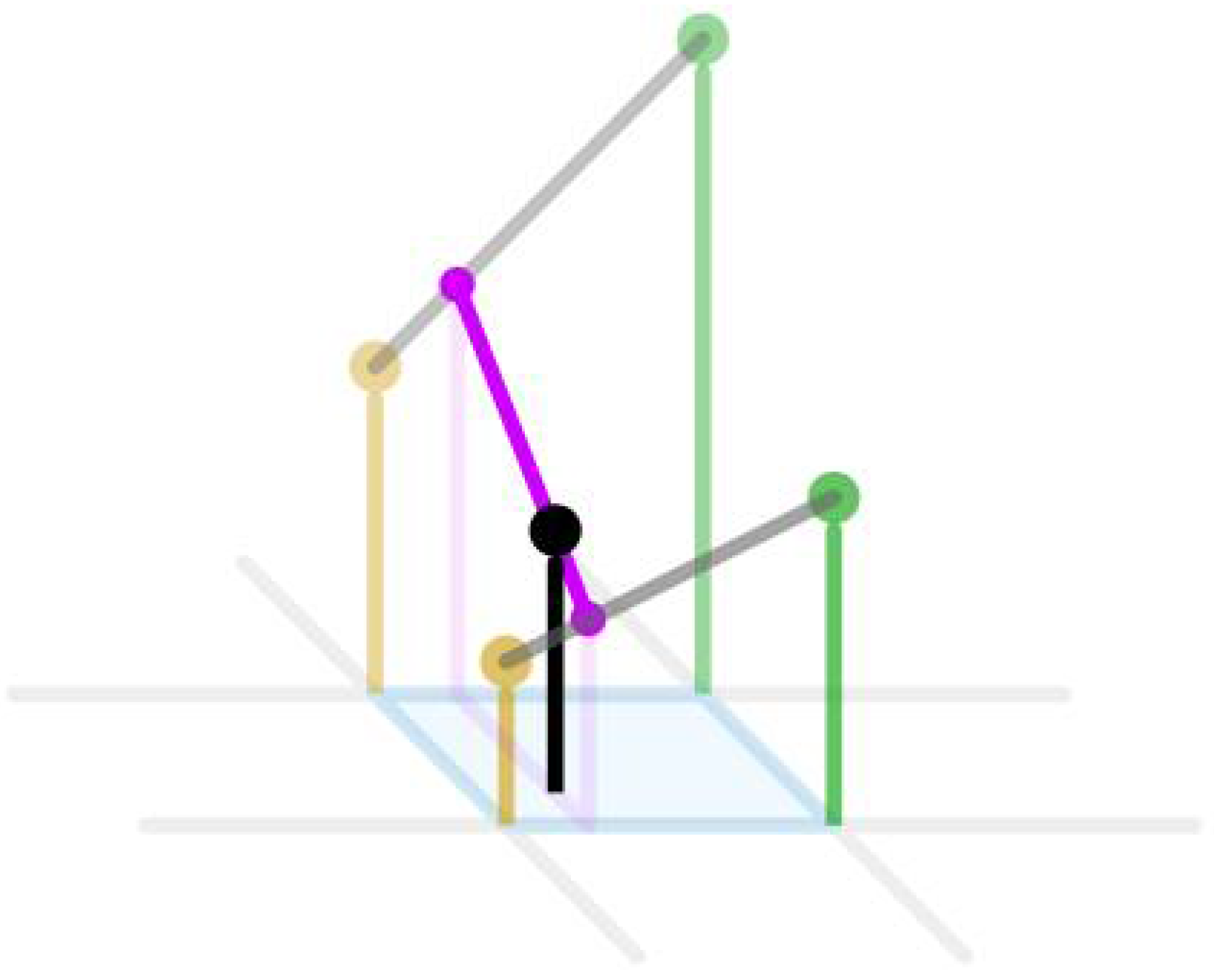
24], was assessed based on 1000 randomly generated ground control points (GCP). A referential value in those points was determined from the original DEM with a resolution of 1 m. Because the new pixel often did not contain the center of the original pixel, the 4 original pixels were taken into account when determining the reference value, and these were calculated using the bilinear interpolation method to account for this offset. The idea of this method is shown in
Figure 1.
The value of a new pixel, shown by the black dot, corresponds to the point being interpolated, and the yellow and green dots correspond to the neighboring samples. Their values correspond to their heights above sea level. Then, at each point, values of all generated DEM were collected and compared with the referential DEM. For assessment of the precision of the height, we used a method which is frequently used in this type of research [
12,
22,
23,
24,
39,
40]—standard root mean square error (RMSE), computed as follows:
where
Z1—the height of the point on the generated DEM;
Zr—referential height of the point;
n—number of control points. This correlates well with a determined value, based on the assessed DEM, and the value of the surface gradient.
2.3. Precision of the Delineation of the Watershed Boundaries
The second element that was assessed was the precision of the determination of the watershed boundaries for all 66 aggregated DEMs. The automatic determination of those elements was carried out in the interface of the SWAT model, which is widely used for modelling of agricultural watersheds. Firstly, watercourses are determined based on the DEM and the threshold value of the drained area where a watercourse is going to occur. This value was selected experimentally so that the watercourses determined based on the original DEM with 1 m resolution were the most similar to real watercourses that occur on a given area acc. to the Hydrological Division Map of Poland. The map was taken as a point of reference because it was created based on the best available materials under the National Research Institute (IMGW) supervision. IMGW is a leader in this field of that research and is widely accepted in Poland as reference material in breeding studies [
41]. A closing point of the tested watershed was a point of crossing of the watercourses determined in such a way, and the boundary of the watershed of the Zgłowiączka River headwaters acc. to the mentioned map. For such a determined threshold of watercourse formation and the closing point of the watershed, boundaries of the watershed with the use of all aggregated DEMs were determined. Then, the surface areas of the obtained watersheds were compared to the surface areas of the referential watersheds from the Hydrological Division Map of Poland.
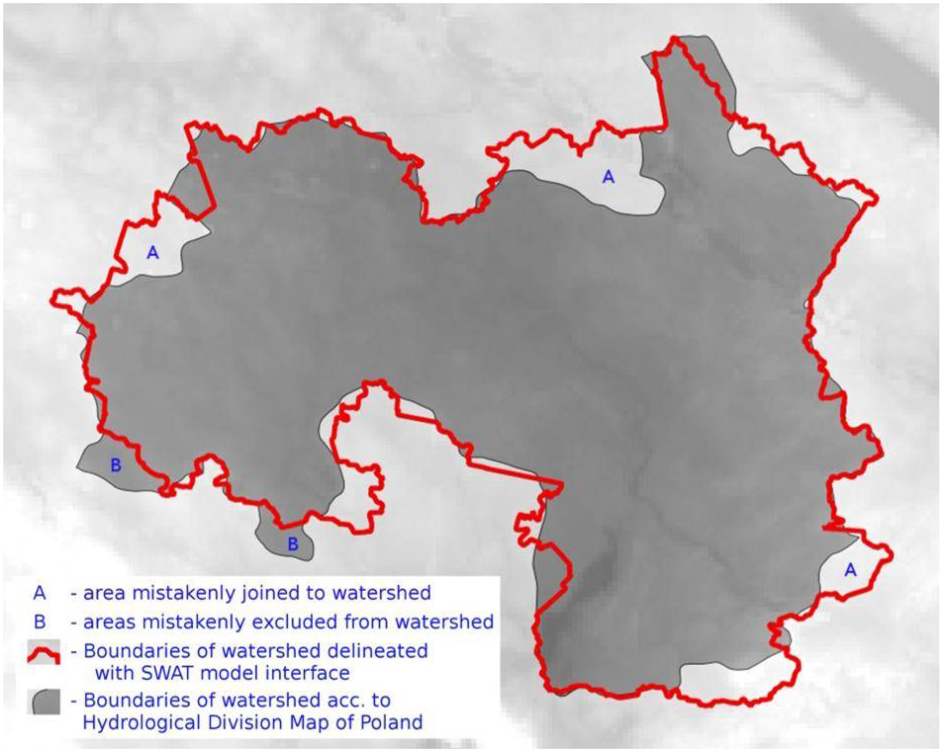
With the automatic delineation of the watershed boundaries in some places, the boundary is outside the real watershed, which leads to the increase in the total surface area. In other places, the determined boundaries cut pieces off the real watershed, reducing a determined surface, which is schematically presented in
Figure 2.
These errors mutually influence the total surface area of the determined watershed, thus a direct comparison of that size to the surface area of the real watershed is not a good indicator of the correctness of the described process. Therefore, it was suggested that both cases were taken into consideration, and only the size of the surface area of the mistakenly determined areas, regardless of the direction of changes, and then divide this by the surface area of the real watershed. The last action enabled us to obtain the indicator of the normalized error area (NEA), which enabled a relative assessment of the correctness of the determination of the watershed, regardless of its size. This indicator was calculated for all the delineated watersheds according to the following formula:
where
Mmod is a modelled area,
Mref a referential area, and ∩ is an operation of the product in geographic information systems.
2.4. Precision of Watercourses Delineation
Delineation of watercourses based on a DEM is the first stage in the entire process of watershed modeling in SWAT. The only element necessary for these parameters is a threshold at which the size of the drained area, the outflow, is going to occur on the flow route. Similarly, as in the case of the boundaries of the watershed—the determination of watercourses based on the original DEMs—this value was determined in a way that the generated river network on the particular area was very similar to the real one delineated on the map. Such a determined threshold value was used for all DEMs with reduced resolution. Determination of the watercourse source location and length is not entirely unambiguous. The lengths of the modeled watercourses depend on the selected threshold, which may cause some errors in the final results. To separate those kinds of errors from the resampling errors, the reference spot is the watercourse. Therefore, the DEM with the highest resolution was recognized as a referential point, and the remaining watercourses were compared to it. Their similarity was assessed based on the length and average gradient.
3. Results
3.1. DEM Precision
Acting according to the above-described methodology, the following list of pixel sizes was obtained—1.5, 2.3, 3.4, 5.1, 7.6, 11, 17, 26, 38, 58, and 86 m. The number of chosen resolutions is clearly larger than the average number obtained by studies with similar topics. Additionally, the largest value is nearly 100 times larger than the original, and it is large enough to allow rapid hydrologic model development of very large rivers.
Then, for each resolution, a DEM was generated through resampling the original one with the use of six methods of aggregation. For the created DEMs, RMSE was computed (
Table 1).
In all cases, the error increases fluently along with the reduction in resolution. The RMSEs for three averaging methods (AVE, MED, and MOD) and the NN method had remarkably similar values, while for the MIN and MAX methods, errors were similar but decisively bigger than those of the four remaining. This difference increased along with the increase in the pixel size. The MIN method obtained the lowest results in this assessment. Only resolution 2.3 m provided a minimally better result than the MAX method.
3.2. Precision of the Delineation of the Watershed Boundaries
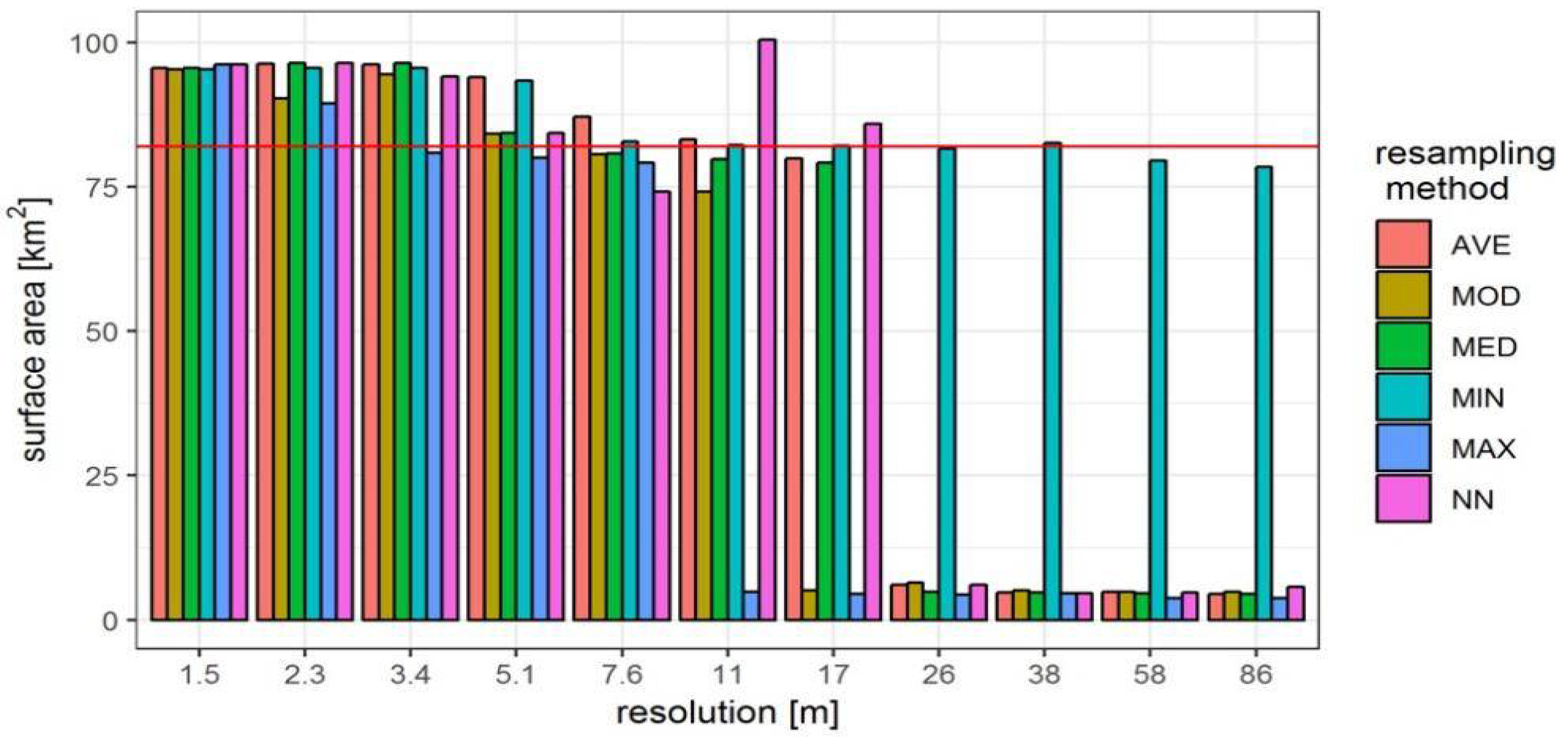
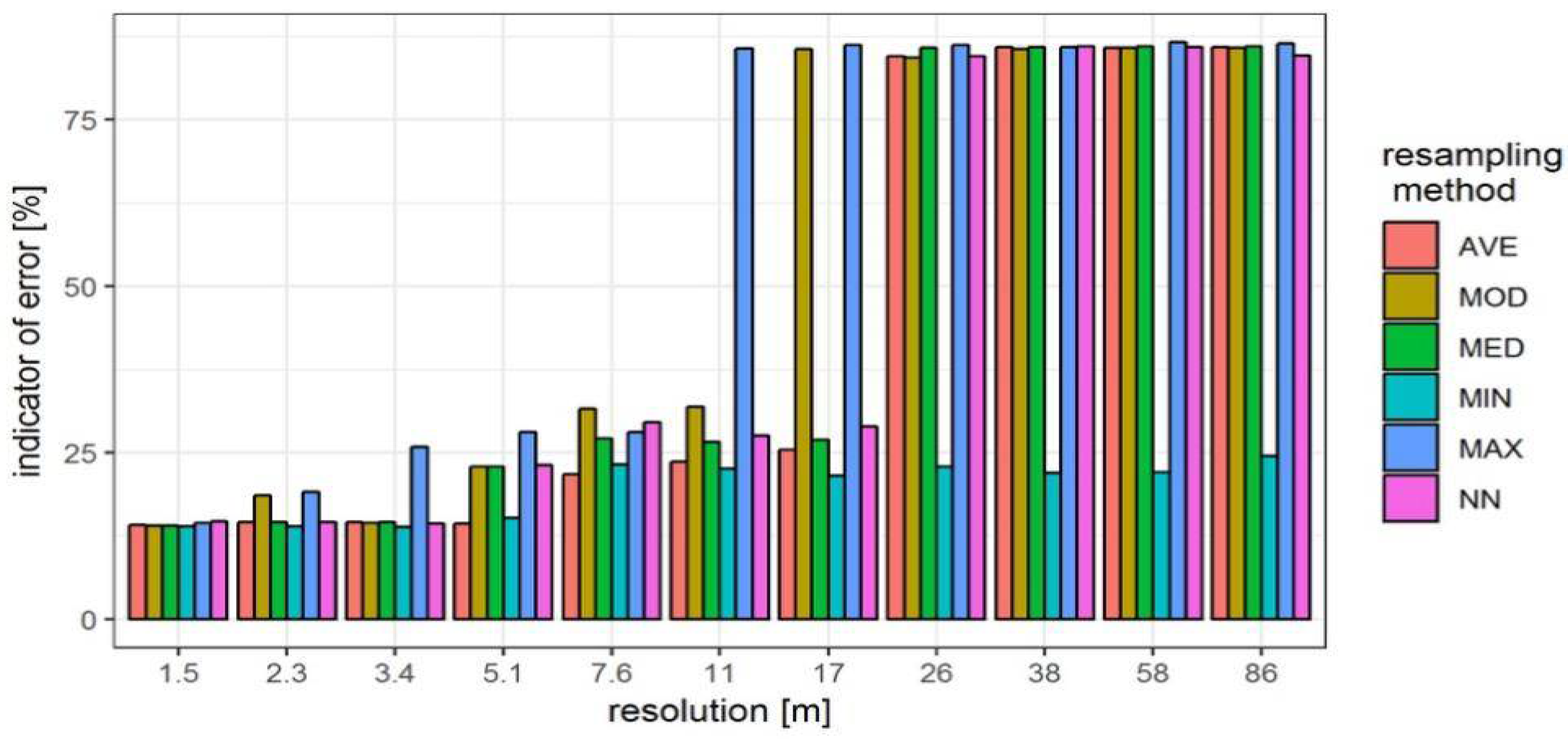
Figure 5 and
Figure 6 present the areas of the determined watersheds and the calculated indicators of the normalized error or surface area (NEA) for the determined boundaries for all the combinations of the 11 resolutions and the 6 resampling methods. NEA is a product of the sum of the surface area of all erroneously determined fragments and the surface area of a real watershed. It is an indicator created by the authors to enable a comparable assessment of the influence of pixel size on watershed delineation. Existing methods did not eliminate the disturbing influence of the direction of changes, and in our study the size of these changes was important—hence, the need for this original idea is clear.
Three ranges of varied dynamics of changes may be distinguished: the first one, from 1.5 to 3.4 m, where errors for five methods (except for MAX) were permanent; the second range was from 5.1 to 17 m, where they slightly grew; whereas in the third scope, from 26 to 86 m, errors were again permanent, but three times bigger than in the case of the resolutions up to 17 m. Results for the MIN method diverge from this rule. They do not differ up to the resolution of 17 m, while from 26 m, they diverge considerably from the others, staying at the same level as for the range from 7.6 to 17 m. For the MIN method, only for resolutions 5.1 and 7.5 m, errors in the determination of the watershed were slightly bigger than in the case of the AVE method. The MAX method at the resolution of 2.3 m had weaker results. The NN method gave slightly weaker results than the best methods only in a few cases, namely for those obtained for the MIN and AVE methods, and in most cases, the results were similar to or better than the MAX, MOD, and MED methods.
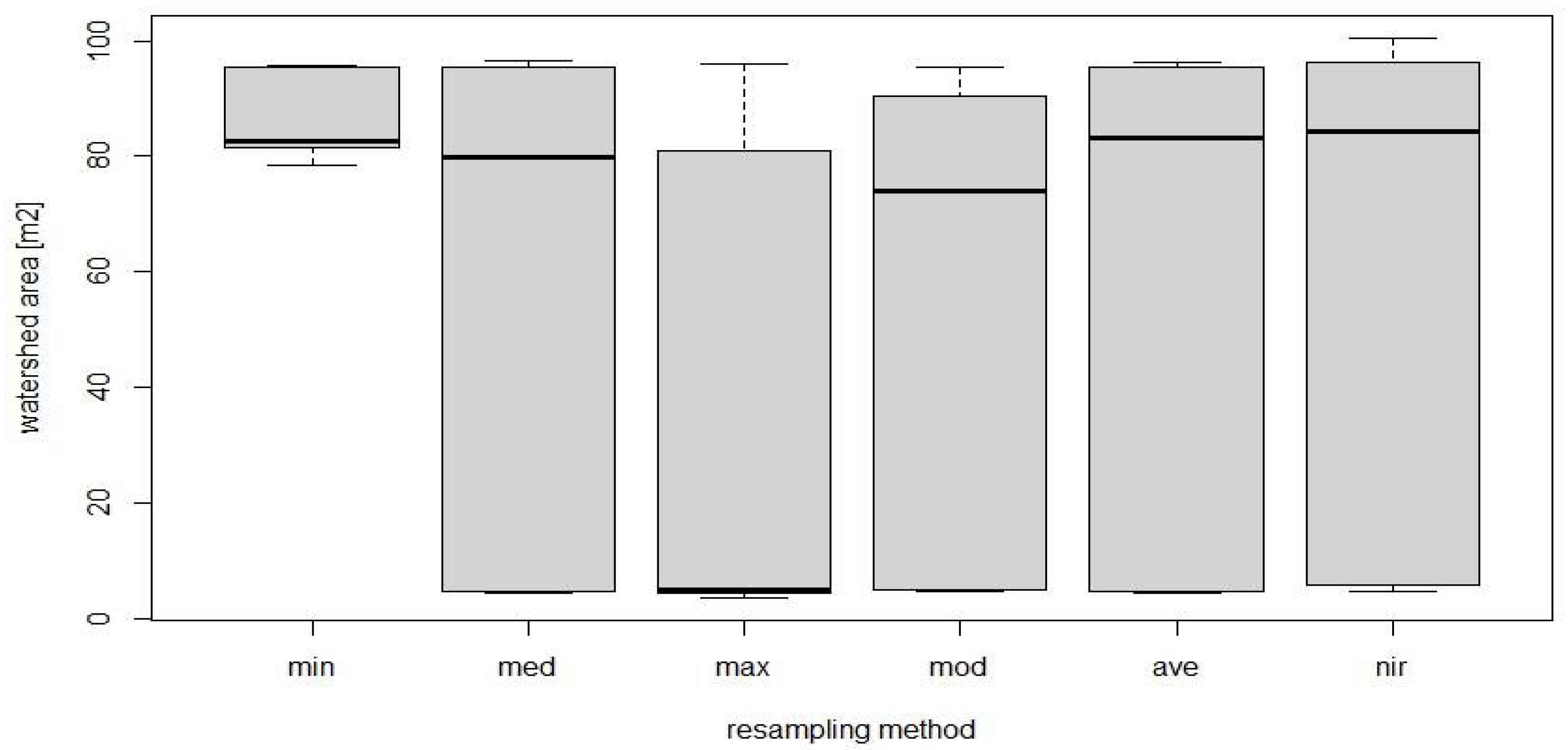
Figure 7 presents a box plot where the
x-axis has the method of aggregation, and the
y-axis gives the area value observed in different resolutions. This chart reveals the min, max, and different quartiles. The box plot allows the variation in the area values in each method to be seen.
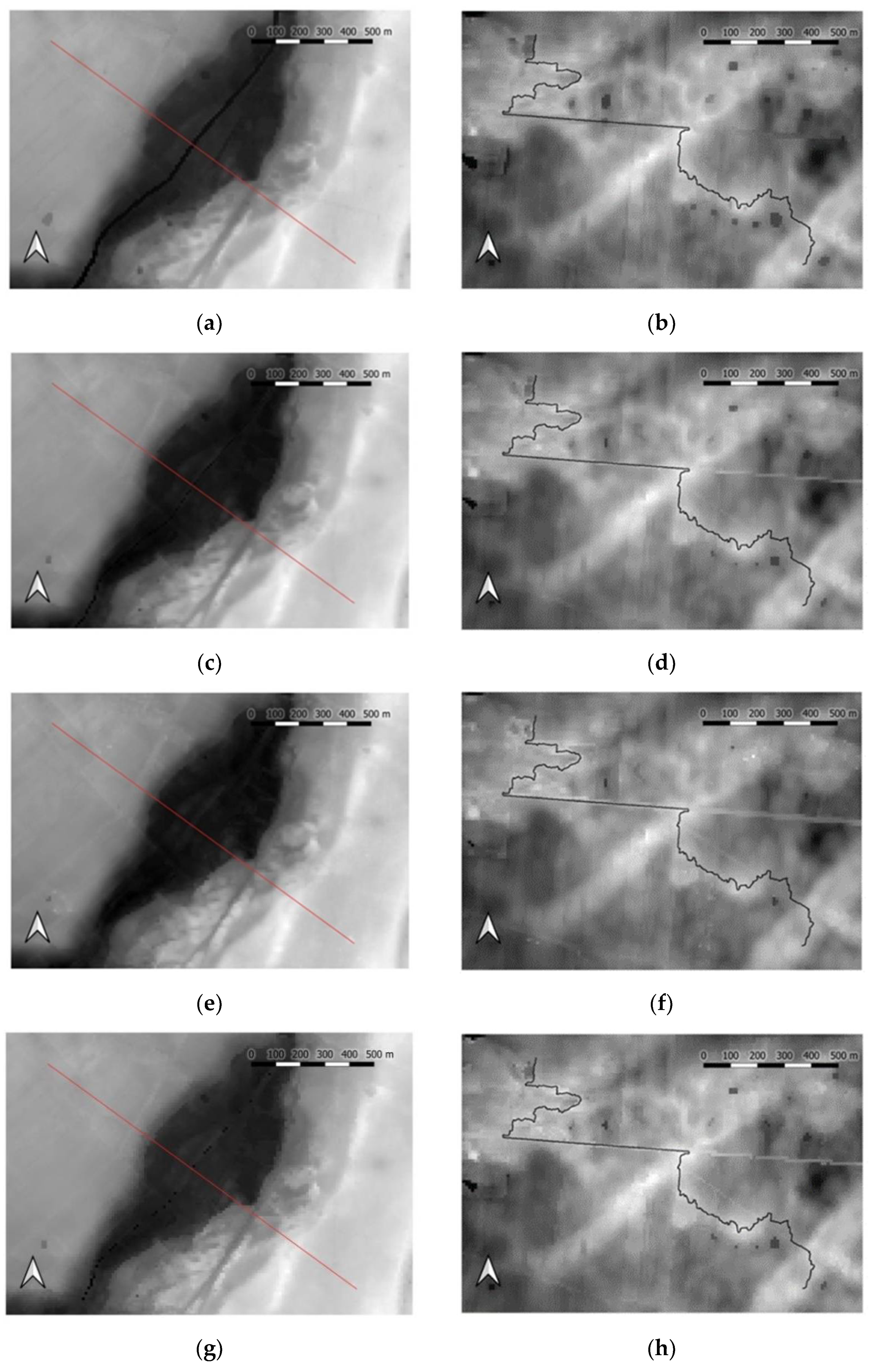
The watercourse drawings with original and reduced resolutions (
Figure 8,
Figure 9 and
Figure 10) for the max method already at a resolution of 11 m (
Figure 9e) do not show the watercourse, and for mod (
Figure 9g), it is significantly interrupted.
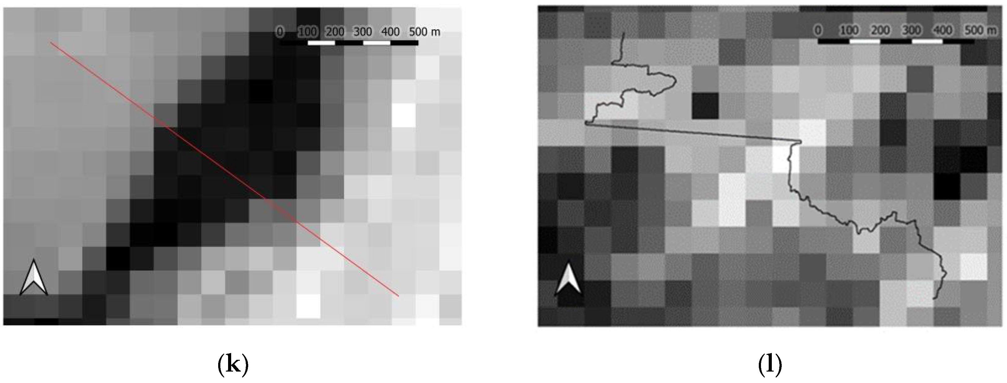
The MIN method (
Figure 9a) clearly widens the stream, its course was not disturbed. Such a result is due to the fact that only the pixels with the smallest value are considered in the MIN method. Conversely, in the MAX method (
Figure 9e), the actual pixels representing the liquid are not considered at all when calculating the value of the enlarged pixel. An intermediate situation occurs in the AVE (
Figure 9i) and MED (
Figure 9c) methods, in which the actual height of the watercourse affects the value of the new pixel but is modified by the pixels actually present in the watercourse edge image.
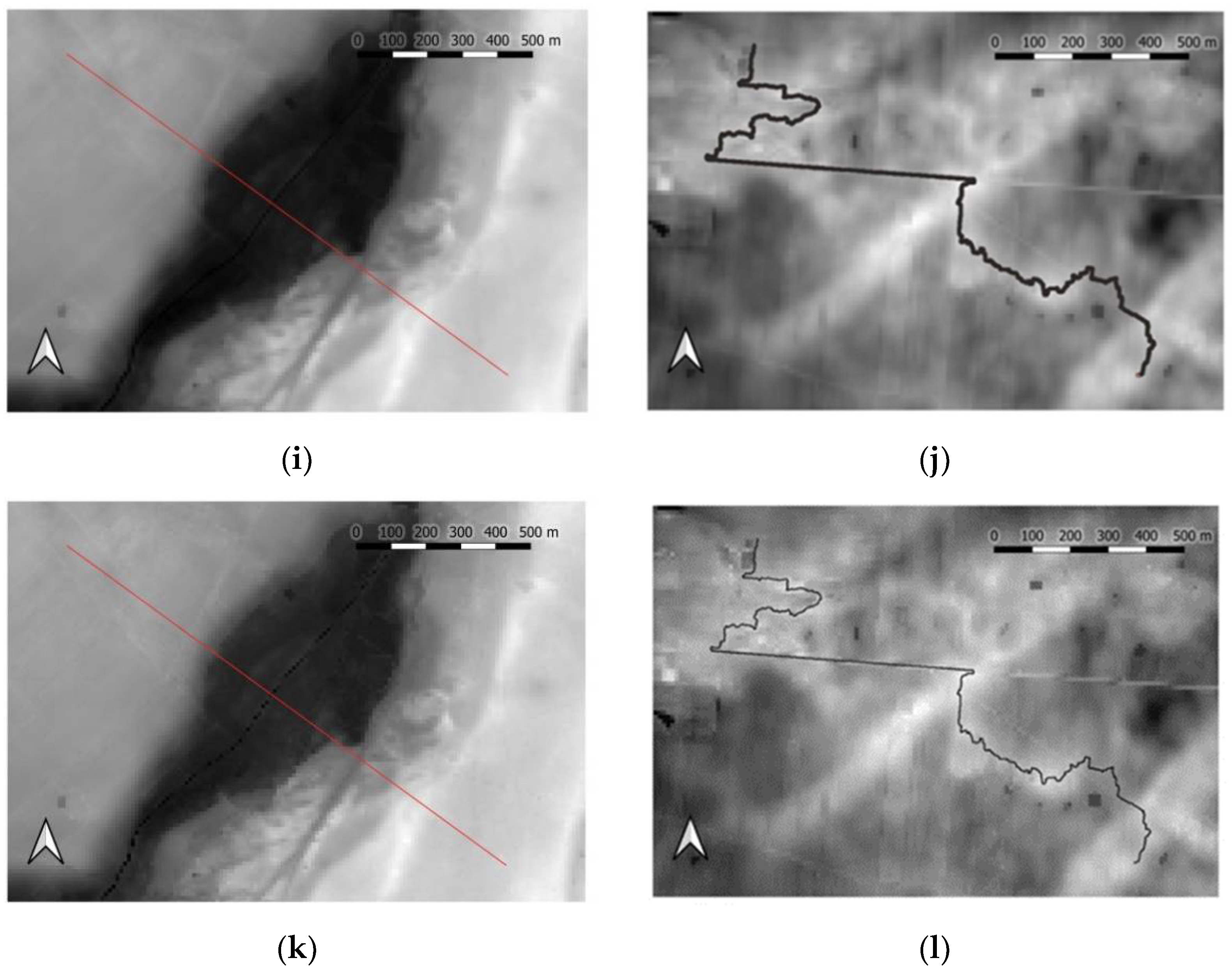
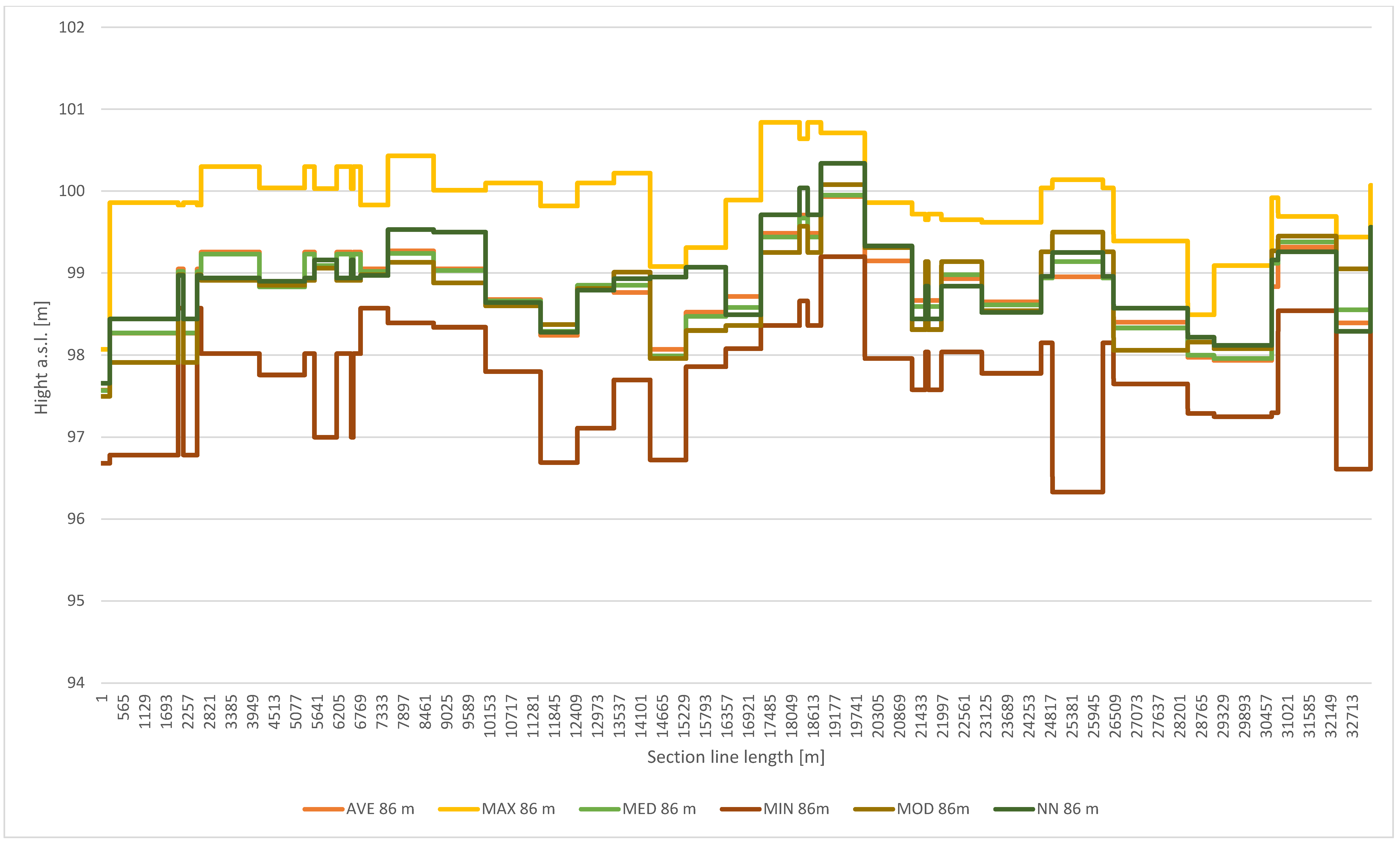
The relationships described above for 11 m resolution occur analogously at 86 m resolution (
Figure 10a). Even at this resolution, the MIN method preserves the shape of the watercourse.
Figure 9 shows the maps obtained with all methods for 11 m resolution, and
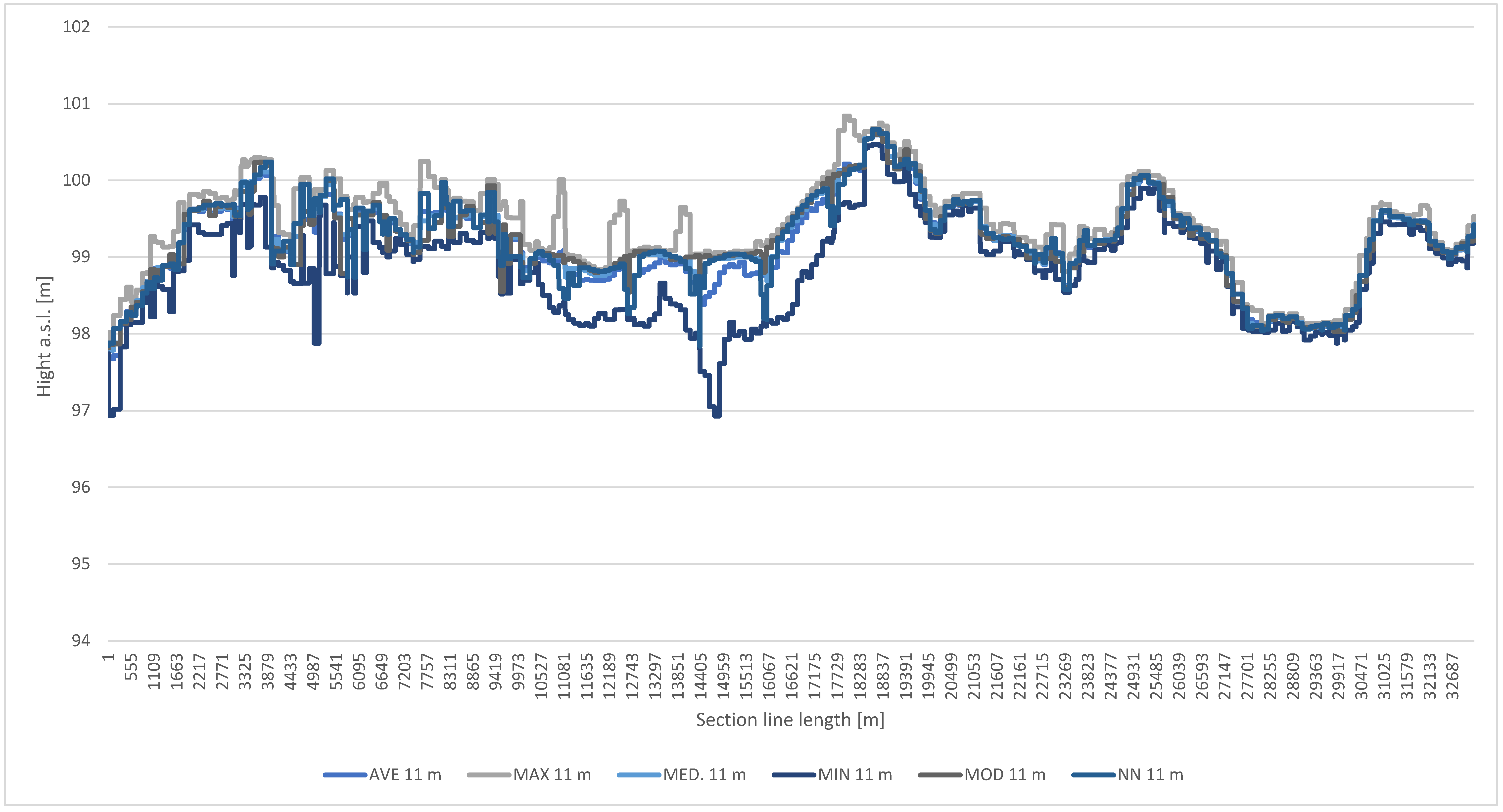
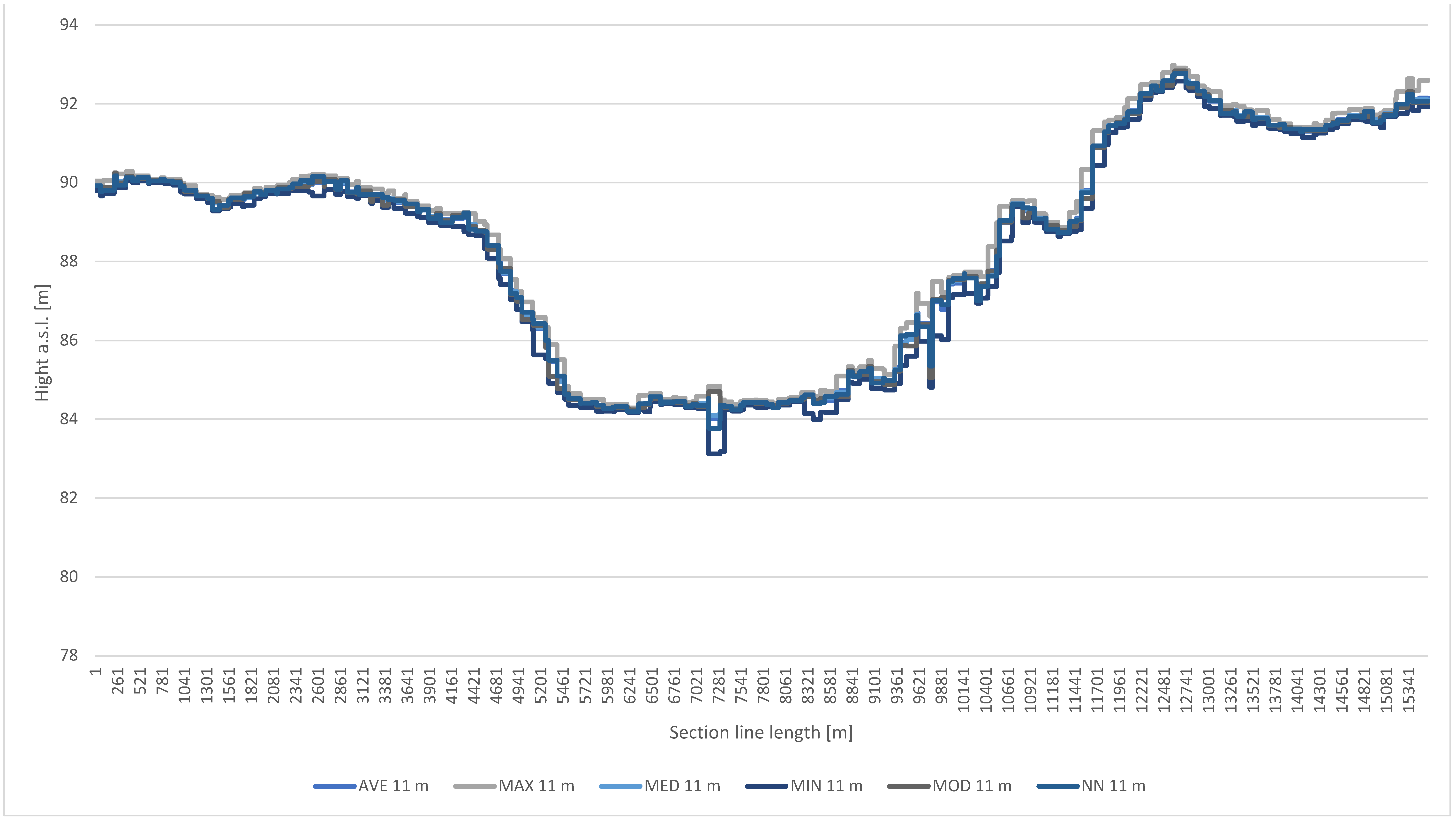
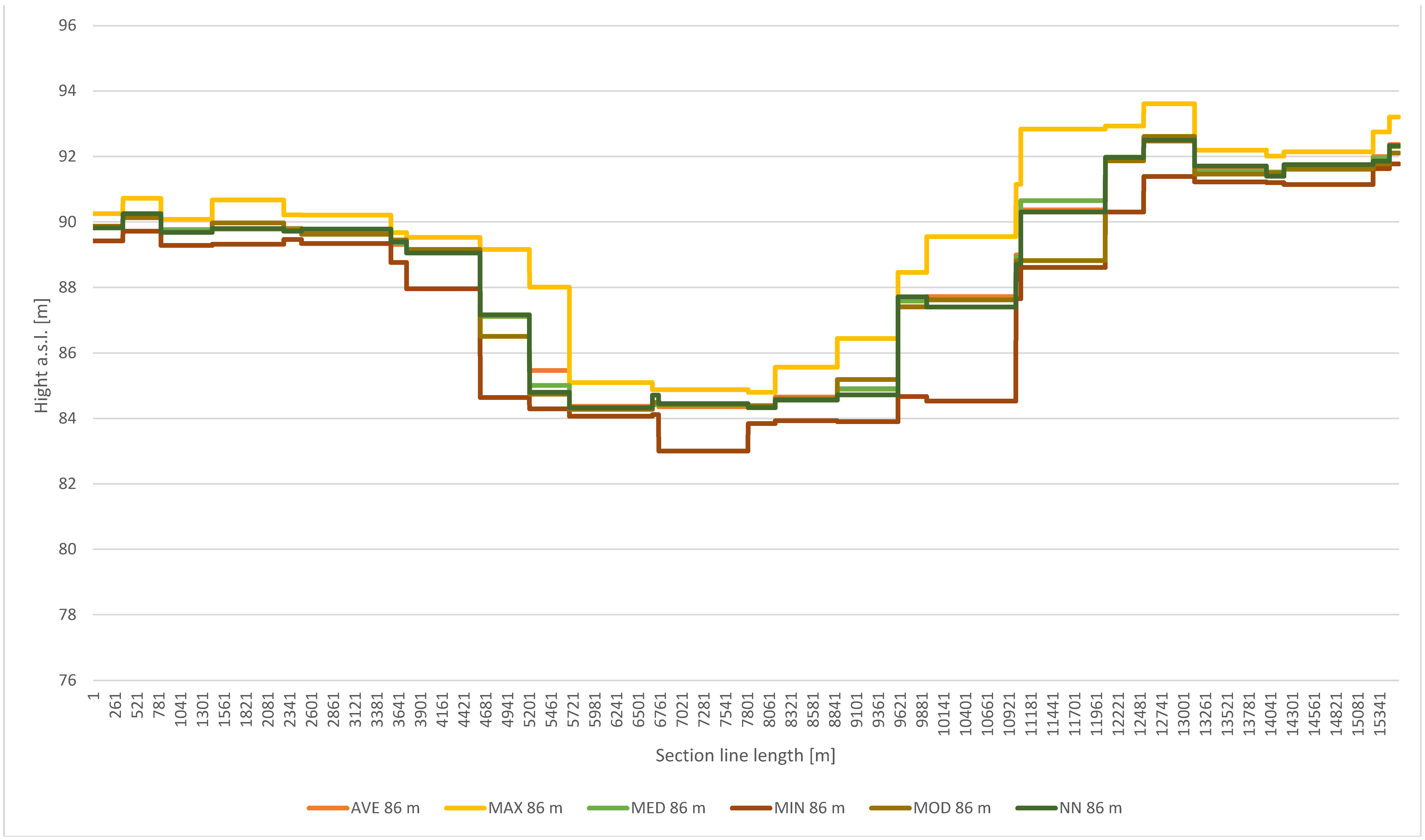
Figure 10 shows the maps for a resolution of 86 m with a marked section line, and the sections themselves—through the watercourse in
Figure 11 and along the ridge in
Figure 12.
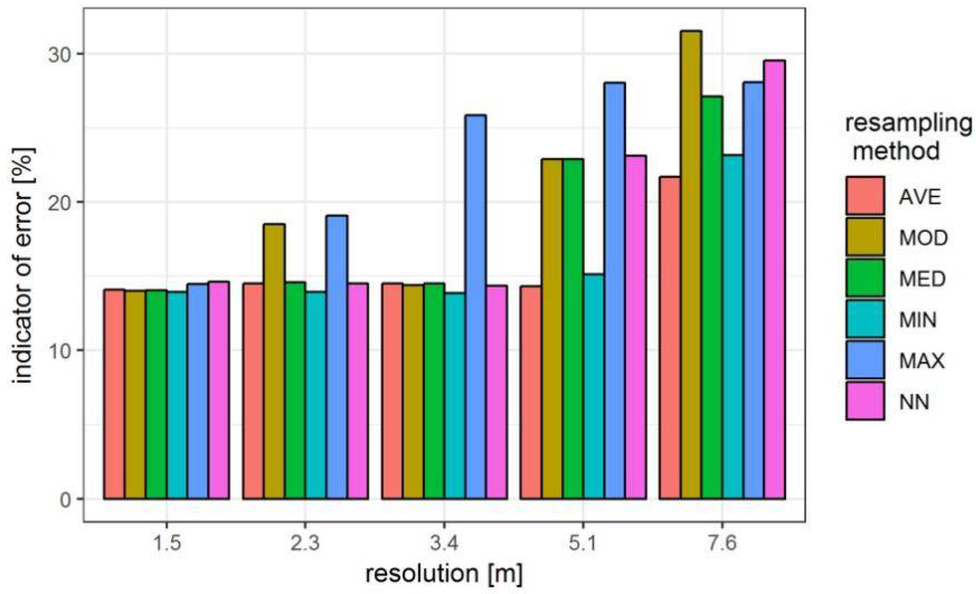
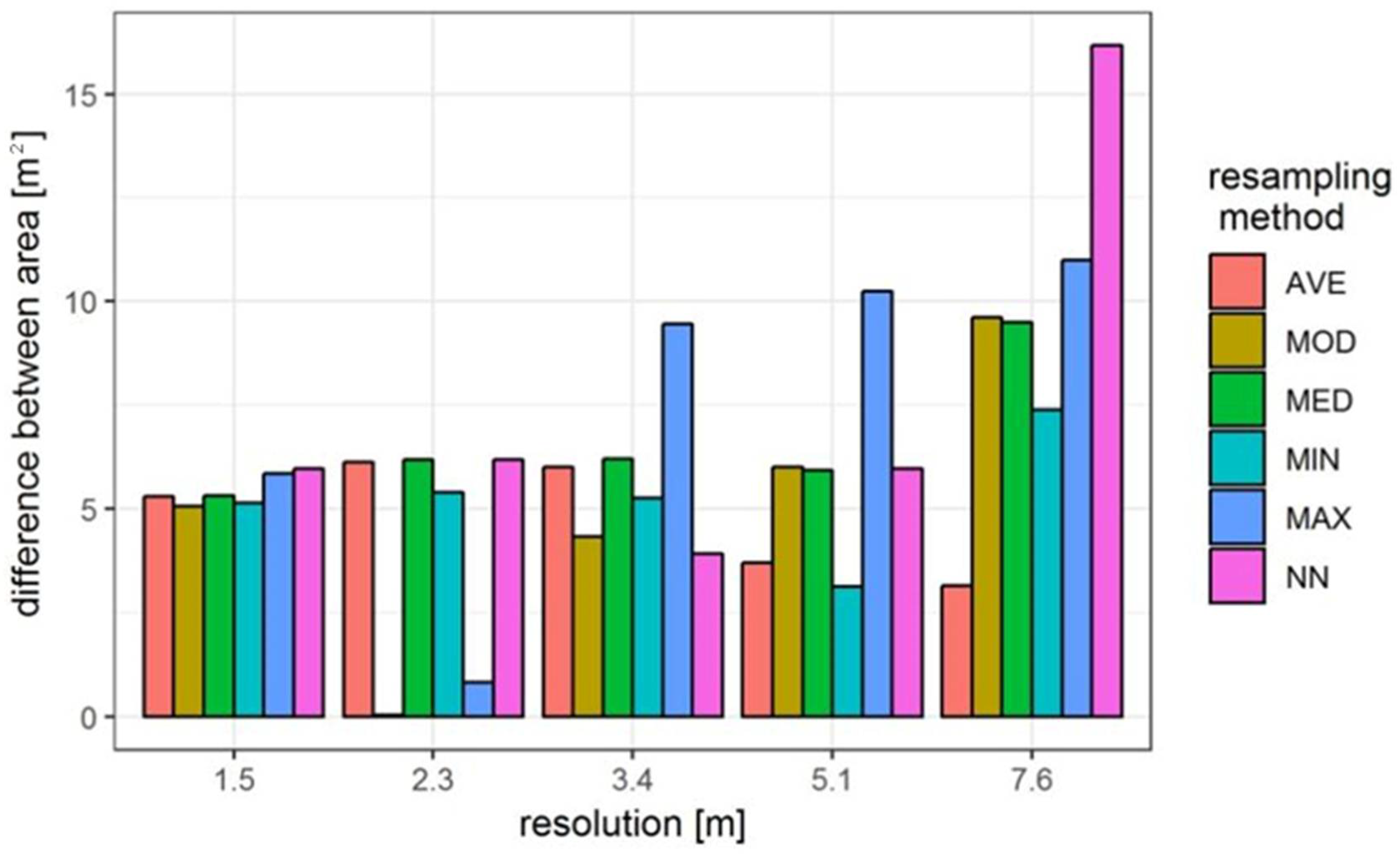
Graphs show the indicator of the normalized area error (
Figure 13) and the differences between the determined and referential watershed (
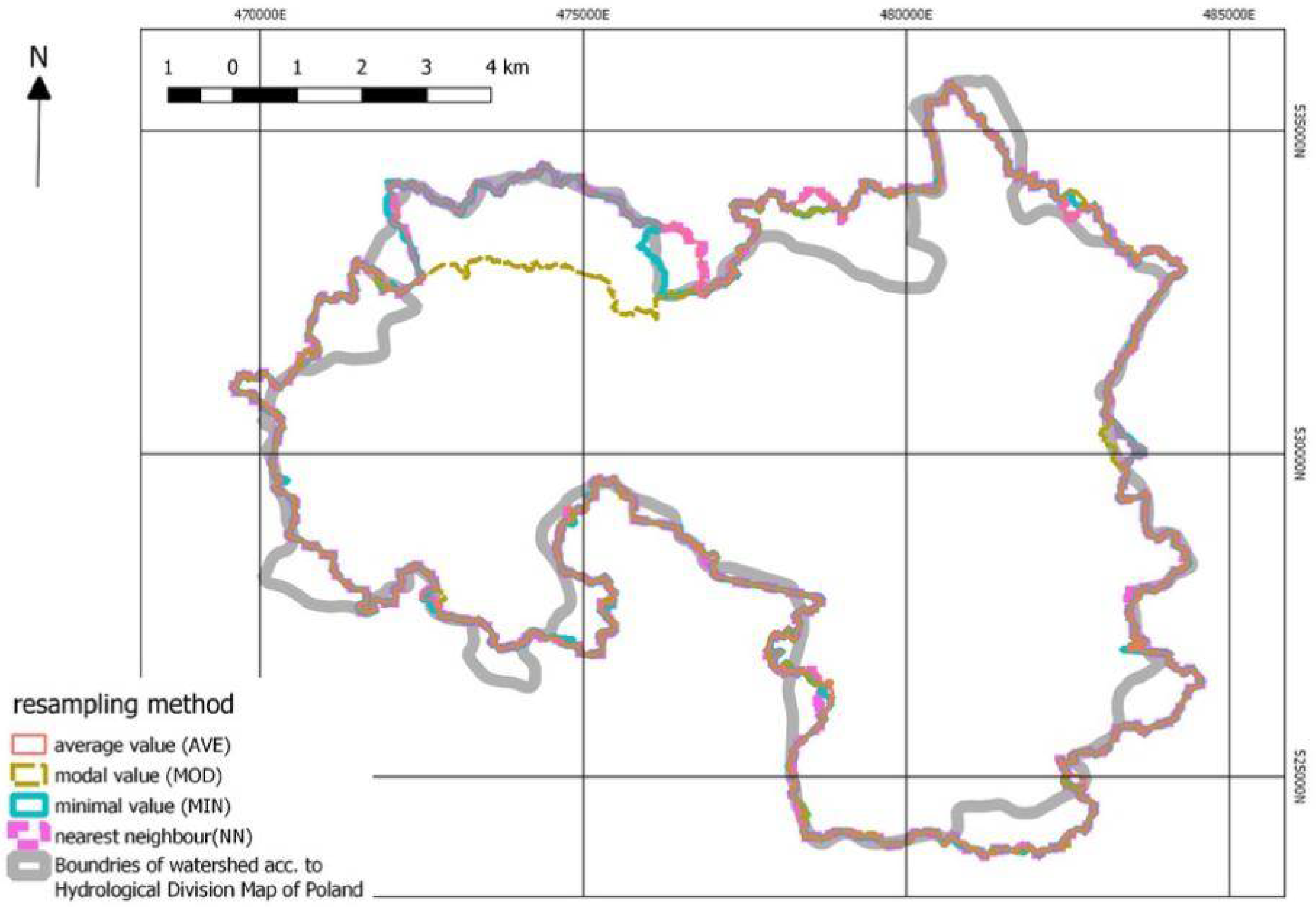
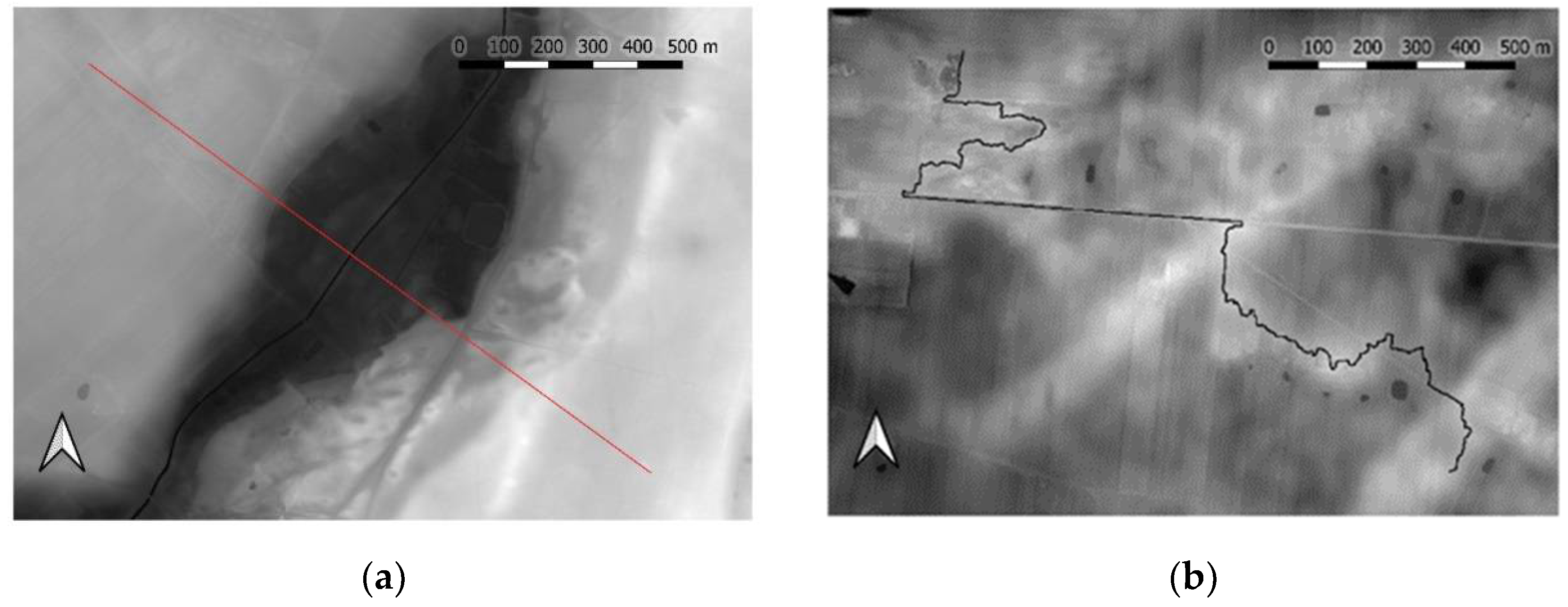
Figure 14) for the DEM resolution from 1.5 to 7.6 m. On both graphs, we may notice a rising trend, but for the indicator, it is clearer and more regular. The advantage of the indicator in the presentation of the precision of boundaries determination is visible in the example of the calculated value for a resolution of 2.3 m. For MOD interpolation, the determined watershed has almost an identical area as the referential one. The difference is only 0.036 km
2, while for the watershed determined based on the DEM after resampling, the AVE is 6.1 km
2. Thus, it may be assumed that the watershed determined with the MOD resampling method is more similar to the real watershed than the results determined with the use of the AVE method. These watersheds are presented in the background of the referential watershed. A vast majority of the generated boundaries are remarkably similar to each other, and the differences are minimal. A decisive difference is noticeable in the northern and western parts. Here, the MOD resampling method resulted in the shift of the determined boundary to the south from its real location, and the cutting of a considerable area, while the AVE resampling method led the boundary more precisely. This error of the MOD resampling method, consisting in the reduction in the area of the watershed, has been reduced by its increase in other fragments. Therefore, all these errors were not detected when areas of watersheds were compared. However, they are taken into consideration for the calculation of the normalized indicator. Thus, a better-led watershed, with the use of the AVE method, obtained a value of this indicator of 14.5%, while the watershed for the MOD method as much as 18.5%.
3.3. Precision of Watercourses Delineation
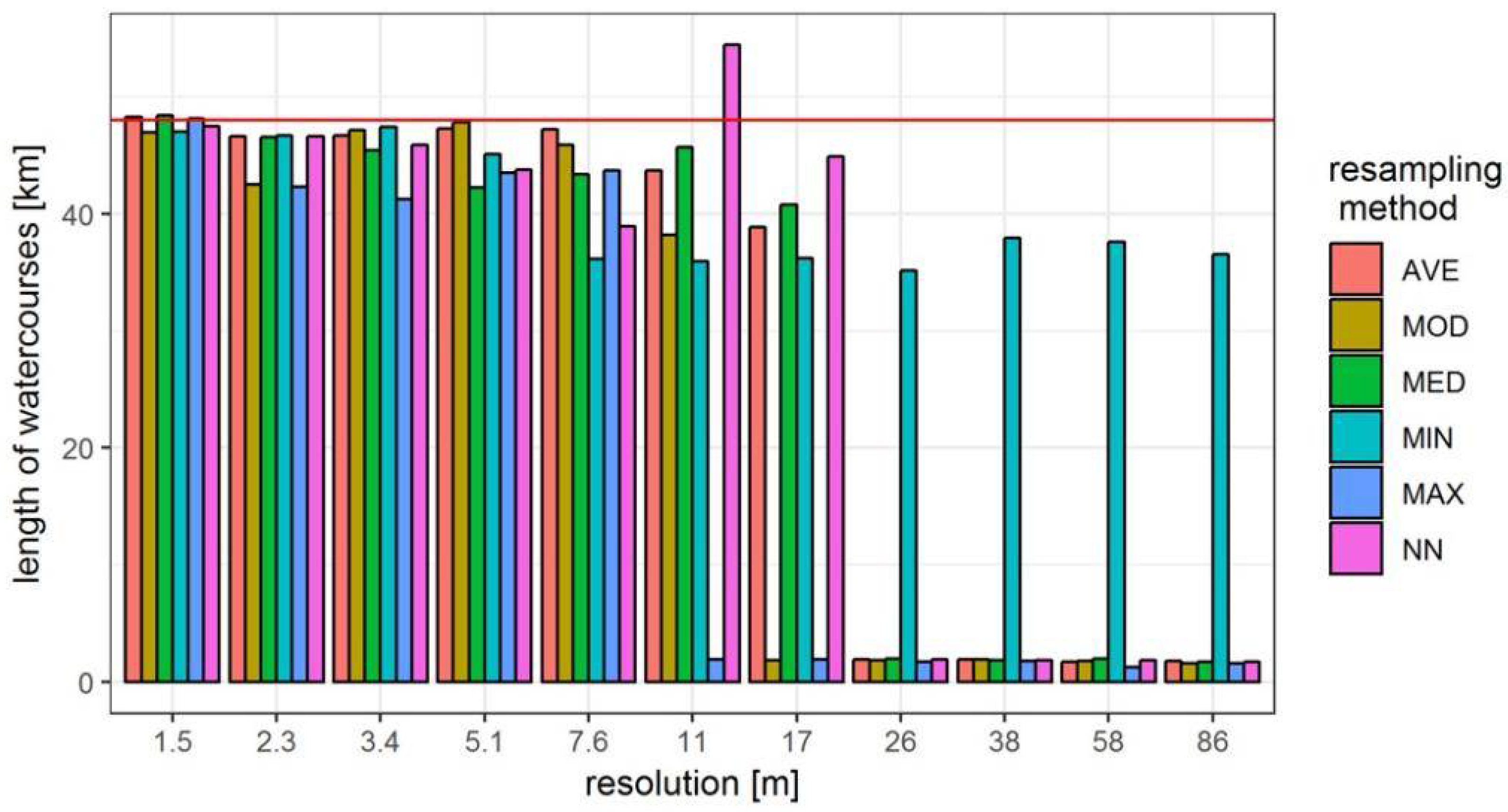
Figure 15 and
Table 2 present the lengths of the watercourses determined with the use of generated DEM for all resolutions and methods of resampling in comparison with watercourses determined based on the original DEM with the resolution of 1 m.
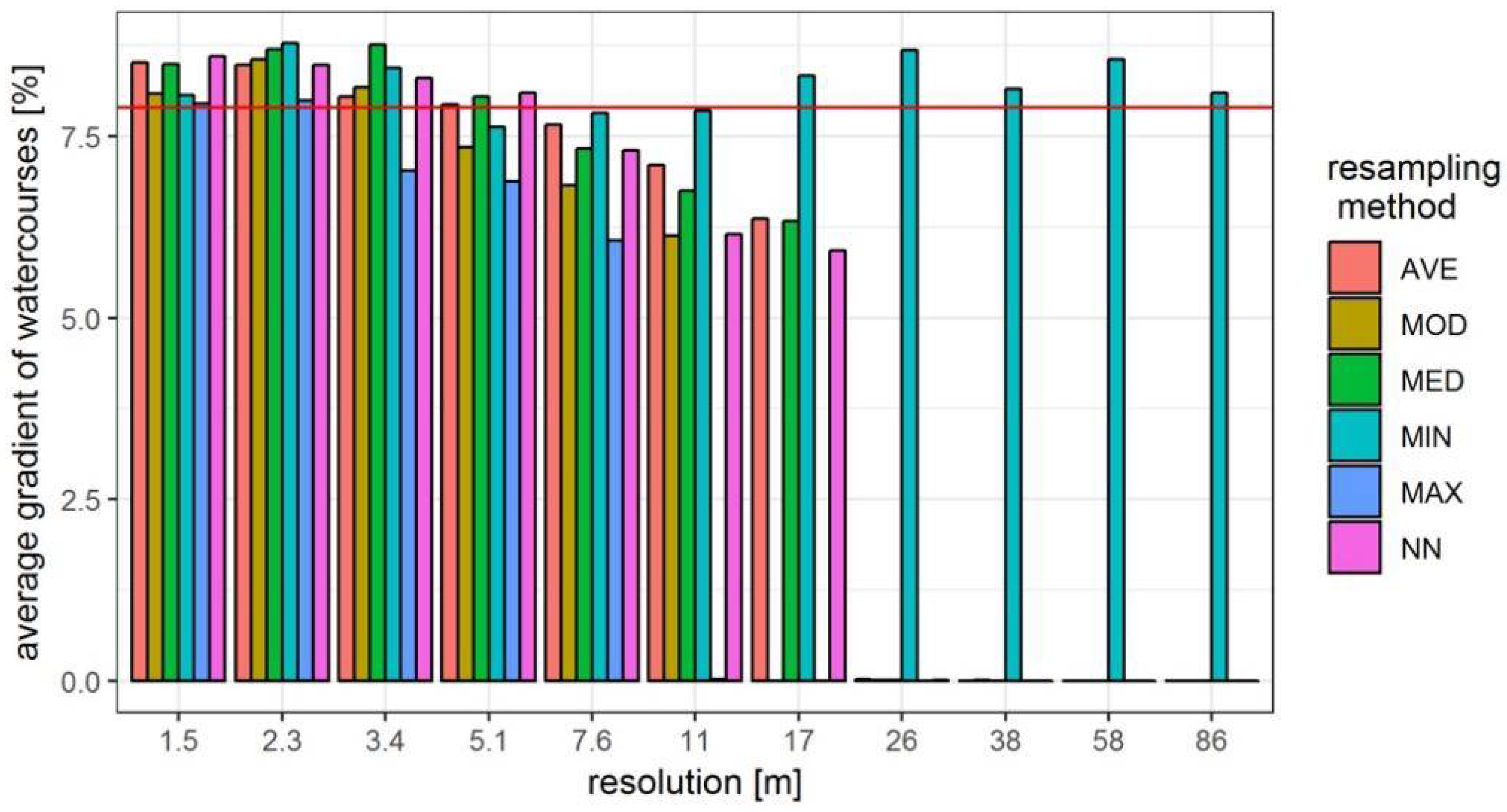
Figure 16 presents average gradients of watercourses determined with the use of generated DEMs for all resolutions and methods of resampling. These values are compared with the gradient of the watercourse determined based on the original DEM with a resolution of 1 m.
Table 3 presents the precision values of the average gradients of the watercourses shown in
Figure 16.
As it was shown in the graphs in
Figure 15 and
Figure 16, both the lengths and gradients of the rivers changed considerably. In both cases, similar to the case of the determination of the border of the watershed, these changes were not uniform. The clearest change was a drastic reduction in both parameters for DEM resolution that exceeds 17 m. It relates to almost all interpolation methods; only for the MIN method did the determined watercourses retain their parameters without any bigger changes for all resolutions. Except for one case, the lengths of the watercourses for all DEMs were shorter than the original one. Initially, at the reduction in the resolution, differences in lengths of the determined watercourses were small and then they clearly increased. The lengths of the watercourses for the MIN interpolation method decreased considerably for resolution 7.6 m (this resolution gives the weakest result among all the resampling methods, but is still maintained at the constant level). Gradients of the watercourses in the initial stage of reduction in DEM resolution rose slightly for all interpolation methods, then slightly but regularly reduced, to drop almost to 0 at the resolution of 26 m. This is not related to the MIN interpolation method, which, from the beginning to the end, fluctuated from around the obtained value to the original DEM.
In the parts of the watercourse presented in
Figure 17 for the MAX method, the watercourse was not visible even at a resolution of 11 m, and for the mode, it was significantly interrupted. The method of means clearly widened the course, but even at a resolution of 86 m, its course was not disturbed. Additionally, on the cross-section through the watercourse (
Figure 18), it can be seen that only for the MIN method was the watercourse depth maintained in both resolutions. The NN and MED methods, although reducing the depth of the trough, did not leave them visible in the same place. In other methods and resolutions, the trough was not visible.
4. Discussion
Many of the tools used and described in the literature are not dedicated to significantly altering the resolution. ANUDEM is a proposition of a commercial, extensive data processing tool that can generate results of various resolutions. Similarly, the resampling tool with the bilinear and cubic methods in ArcGIS is also not dedicated to significantly changing the resolution. When changing the resolution from 1 m to 50 m, we make 1 pixel out of 2500 pixels. There is no significant difference in the result, whether we take 1 pixel (NN), 4 adjacent pixels (bilinear), or even 16 (cubic) pixels for the calculation compared to the other option, of taking more than 2480 distant pixels. Therefore, in this paper, statistical sampling methods were used. The operation modes have the same characteristics regardless of which is chosen, when the size of the resolution change is not taken into account.
4.1. DEM Precision
The results obtained in these studies decisively diverge from the ones obtained by Haile and Rientjes [
23], who applied, inter alia, the NN method for reduction in DEM resolution.
Table 4 presents the results of the comparison.
When the length of the pixel edge increases by threefold, the results in both cases are close to three. In the case of a fivefold increase, the RMSE obtained by Haile and Rientjes is considerably lower, but the trend is the same, because in both cases the RMSE increased. On the other hand, at the sevenfold change in resolution, the RMSE in their studies was not only much smaller than the RMSE in these tests, but it was the smallest of all the cases described in this paragraph. Despite only three resolutions being investigated in the research by Haile and Rientjes [
23], it is clear that the relation of the DEM error to its resolution is not rectilinear or even monotonic. An analogous situation was shown for the bilinear situation and the cubic convolution. In these studies, in no cases did a change in the trend occur or an error regularly increase along with the increase in the DEM resolution.
Chen et al. [
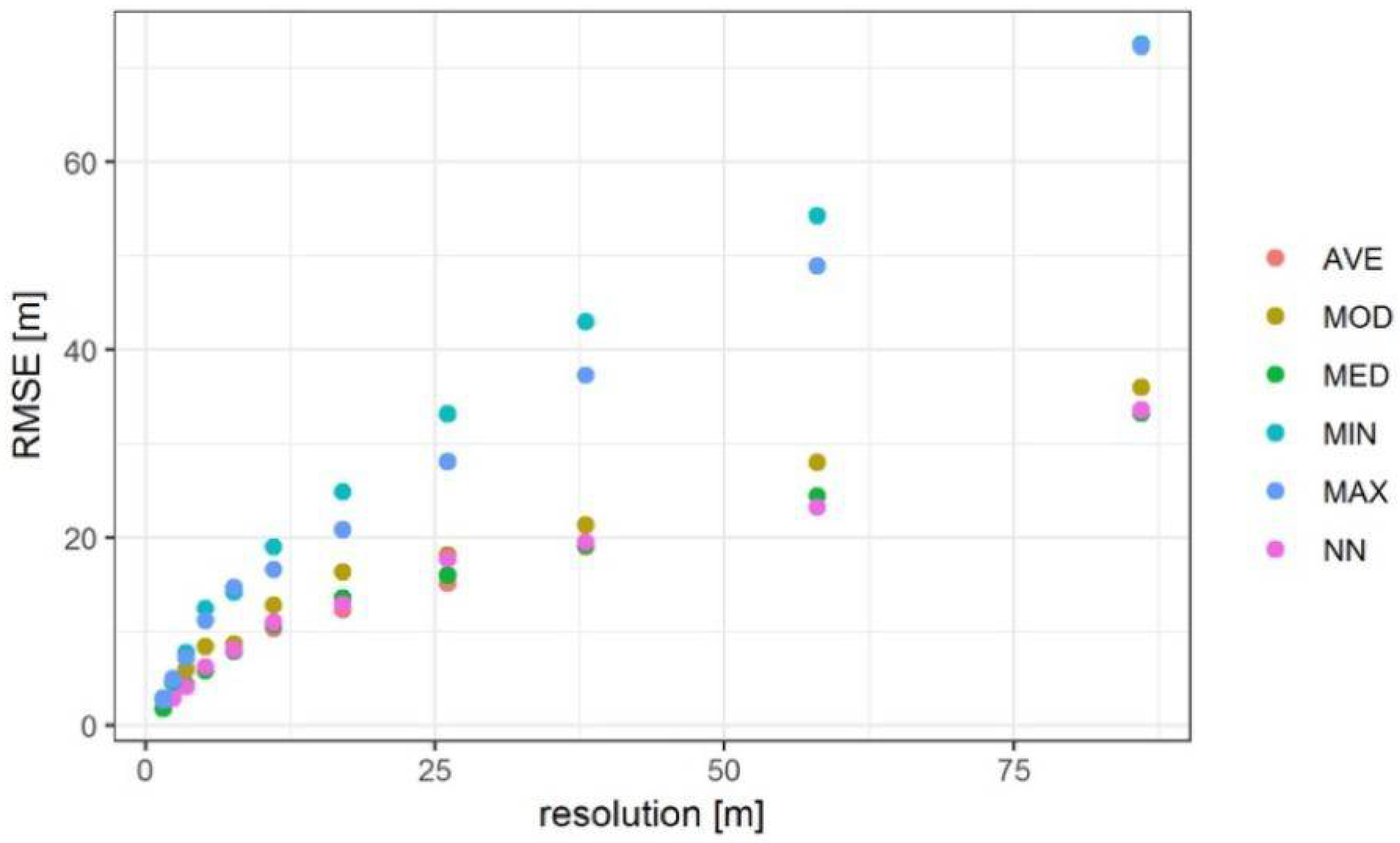
42] analyzed DEM precision with an original resolution of 3 m aggregated with steam burning, ANUDEM, and Compound methods. The calculated values of RMSE were close to the ones obtained in these studies at the comparison of the results for aggregated DEM, where the pixel edge was the same multiplicity as the original one. In both cases, the error systematically rose along with the pixel size. Chen et al.’s results may be assessed from the point of view that, in the range investigated by them, the RMSE depended linearly on the resolution, while in this paper, for DEM resolution from 11 to 86 m, this relation has an elementary dependency (
Figure 19), and the error depends linearly on the resolution, as in the case of Chen et al. [
42].
Thus, one may assume that the results of these papers differ only because a varied range of resolutions was taken into consideration.
4.2. Boundaries of Watershed
Lin et al. [
22] carried out analyses for DEM from three various sources and using resolutions of 5.30 and 90 m. These were, respectively, DEMs made based on topographical maps on the scale of 1:10 000, and DEMs from the Aster device and SRTM mission. The authors reduced the resolution of private data to 140 m, obtaining 11 diverse sizes of a pixel. In the entire scope of changes and for all sources, the surface areas of watersheds remained unchanged. Similar studies were carried out by Dixon and Earls [
2], who reduced DEM resolution from the original one of 30 m to 90 and 300 m. At a tenfold reduction in DEM resolution, the surface area of the determined watershed decreased by less than 2.5%. The trend of changes was the same as in this paper; however, the differences obtained by them was slight. Both the results of Lin et al. [
22] and Dixon and Earls [
2] are similar to the results of this study in some ranges of the change in DEM resolution.
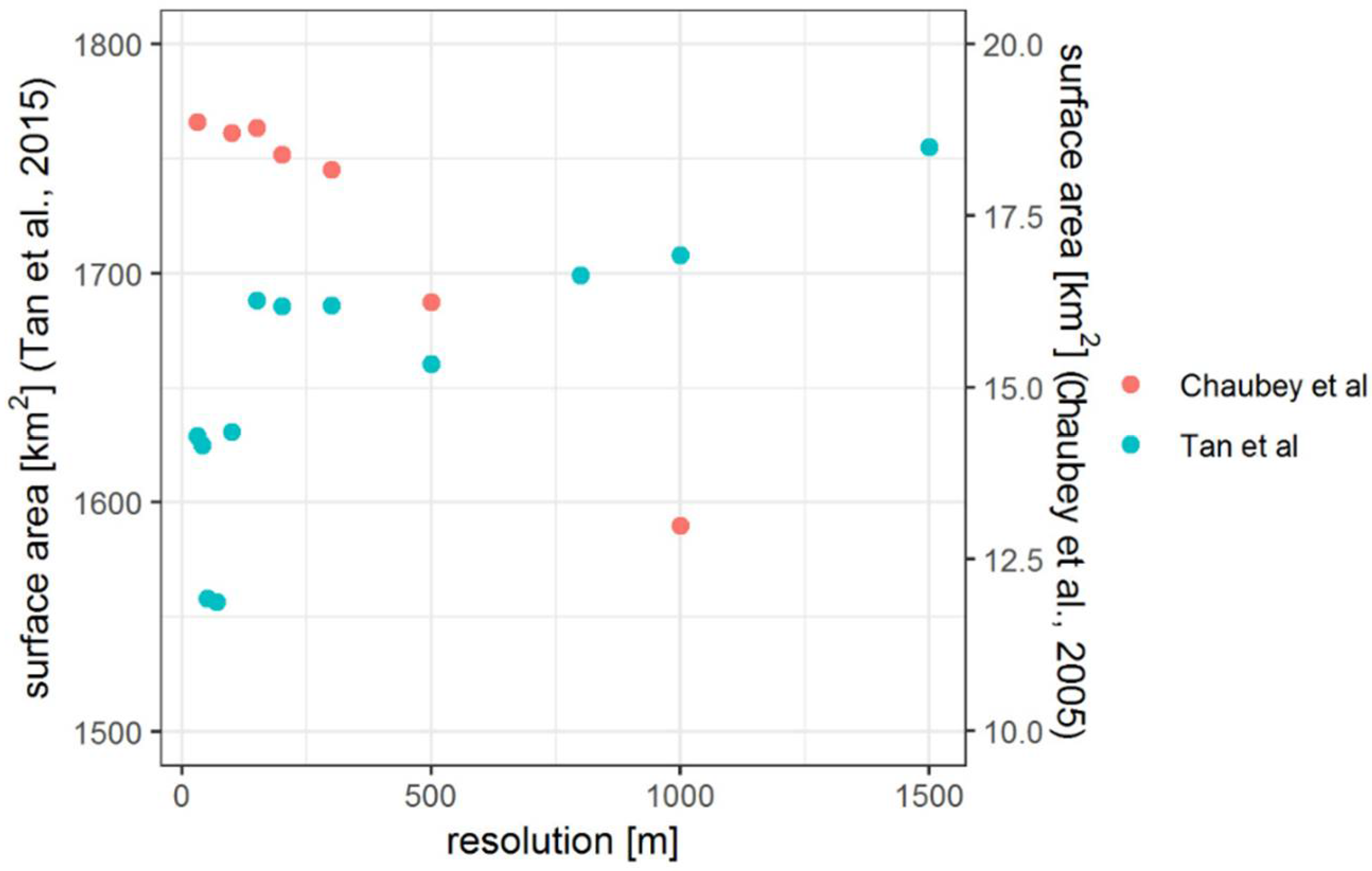
Chaubey et al. [
43] increased the size of a pixel from the original 30 m to, respectively, 100, 150, 200, 300, 500, and 1000 m using only one method—bilinear interpolation. Along with the decrease in resolution, the size of a given watershed systematically decreased, which is presented in
Figure 20. These results are also similar to a fragment of this research (DEM resolution: 3.4–17 m).
Another characteristic of the changes in the surface area of the watershed was obtained by Tan et al. [
24]. In their case, the surface area of the watershed increased (
Figure 20). With smaller changes in the resolution, the dynamics of changes in the surface area were significant, and when reaching a higher size of pixels, changes reduced considerably.
Charrier and Li [
1] used DEM from LiDAR measurements with an original resolution of 1 m, reducing it later to 3, 5, 10, 15, and 30 m. They noticed that, in the case of the highest resolutions, 1.3 and 5 m, there were errors in the determination of the watershed boundaries that disappeared at larger sizes of pixels. They suspected that it may be related to the impact of small forms in the topography of the terrain, such as roads or bridges, on the DEM shape, which at smaller resolutions can be insignificant due to the average value of pixels. According to the author, this is an issue of mistakes in the preparation of the DEM, which is a subject of separate studies [
44], and not an issue concerning the impact of its various resolutions on the determination of the watershed boundaries.
Based on LiDAR measurements, Goulden et al. [
27] made DEMs with resolutions from 100 to 1500 m and analyzed, inter alia, their impact on the area of the determined watershed. Errors in the determination of boundaries were generally small, but the authors noticed that they clearly rise when the DEM error exceeds the difference in the height of neighboring pixels. Such boundaries also occur in these studies, but we failed to find the reasons for their occurrence.
In both the described and previous studies, we cannot notice a clear regularity of the impact of the DEM pixel size on the change in the watershed size. Its surface area may stay almost constant [
2,
22], may change fluently [
43], or may change irregularly—in a step manner [
24], this study.
An indicator similar to the NEA indicator suggested in
Section 2.3 was used by Charrier and Li [
1] and previously by Bates and De Roo [
45], as follows:
where
Mmod is the modelled area,
Mref is the referential area, ∪ and ∩ are the operation of the sum and the product in geographic information systems, respectively. Errors of the watershed increase by a value which has a smaller impact on the size of the indicator than the reduction in the watershed by the same surface area. In the suggested indicator, the basis for normalization is a surface area of the real watershed, and both types of errors are treated the same.
4.3. Watercourses
Wu et al. [
26] decreased an original resolution of 10 m to 30, 60, 100, 150, and 200 m with the nearest neighbor, bilinear, and cubic convolution methods. They analyzed the longest flow paths, which were the same as the determined watercourses at the minimal surface area of drainage required for the formation of the outflow. For all ranges of changes in resolution and resampling methods, the flow paths changed considerably. However, contrary to these results, one could not have noticed any correlation of these parameters.
Yang et al. [
19] performed various DEMs from measurement points made with LiDAR. They determined watershed and watercourses for DEM with resolutions of 1, 5, 10, 30, and 60 m, and then compared them with a determined model from the field data. They analyzed, inter alia, the length and gradient of watercourses. The watersheds taken into consideration were mountainous, and for various DEM resolutions, the determined watercourses were remarkably close to each other and crossed regularly. In these studies, changes in parameters of the determined watercourses were much higher than in the research by Yang et al. [
19]. They were aware that such results could not be reached for watersheds with smaller gradients, and they confirmed that, for such terrains, issues related to the delineation of the boundaries of watersheds and a river network are inseparable.
The impact of both resolution and the resampling method on the length and gradient of watercourses was the subject of the research by Tan et al. [
24]. They took into consideration the nearest neighbor, bilinear interpolation, cubic convolution, and majority methods, which they used for the change in DEM resolution from 20 to 60 m. Unfortunately, this change in pixel size did not show any impact on the obtained parameters of watercourses. These results differ from the above, but it may be assumed that this is a product of using DEM analyses of 11 new resolutions instead of only 1. For the change in resolution in a wider scope, as much as up to 1500 m, Tan et al. [
24] used only the NN method. The length and gradient of the watercourses determined based on the DEM, obtained in such a way, changed irregularly, and no clear relation was noticed.
Comparable results were obtained by Charrier and Li [
1]. They obtained regular reduction in the length of watercourses along with the reduction in DEM resolution. Similarly, they used the source LiDAR DEM with a resolution of 1 m. The results obtained therefrom were used by them as a reference, and they made tests for several DEM with slight differences in the resolution.
4.4. Discussion Summary
Due to the large scope and frequency of DEM resolution changes, the results of this study could not fully coincide with the previous ones described in the literature. However, it can be noticed that most of them coincide with fragments of the results of this work. Together, they can create one coherent picture, in which, along with the reduction in the DEM resolution, there are alternating periods of decreasing and constant modeling accuracy.
Cases of increasing modeling accuracy along with decreasing resolution are rarely described in the literature. Such cases were noticed in the described studies, but they resulted from errors in the DEM. After eliminating them, the change in accuracy returned to the expected one.
5. Conclusions
Generally, problems of hydrological modeling related to the precision and resolution of DEMs are related to watersheds with a small gradient of the terrain. In mountainous watersheds, shifts of the watercourses or boundaries are small, and most often are related to the generalization of the shape within the range of the pixel size.
On the DEM, errors in the form of no correction of the height of some buildings and structures such as bridges and culverts may occur. High DEM resolutions may cause considerable errors in the determination of the watercourses and the boundaries of watersheds. At lower resolutions, this effect changes, and the error related to the resolution decreases. This change may be bigger than the increase in the error related to the reducing DEM resolution and, after placing these effects, within this range of resolution, the precision of modeling may increase along with reduction in resolution, which may lead to erroneous general conclusions being drawn.
The size of the watershed is not the best indicator in assessing of the usefulness of a DEM in determining the watershed boundaries; thus, NAE indicators were suggested, where boundaries shifted to the inside and outside of the real watershed do not level each other out, and the impact of the first and the others depends on the equal weight.
In the assessment of the resampled DEM—by comparison of the value with the referential value—the weakest results were obtained by the MIN method, while in the assessment of the precision of the determination of watercourses and boundaries of the watersheds, this method obtained the best result. This results from the fact that not only the method of the resolution change, but also the assessment method of its operation, should be adjusted to the manner of use of the resulting DEM.
In the entire range of the DEM resolutions, there were fragments with various dynamics of the change in the precision of the determination of the watershed and watercourse parameters. For some fragments, these parameters changed slightly or not at all, and for others, changes were regular and fast. There may be several different fragments, thus, a high sampling rate is needed for their detection. In this research, another DEM was obtained by division of the resolution of the previous by 1.5. Probably, similar analyses carried out on other watersheds, or with the use of this factor, would enable a better explanation of this phenomenon. Recognition of the rules that govern the dynamics of the changes in the precision of modeling watersheds would enable indication of some values at which an increase in the DEM resolution gives small advantages, or where the relation between the quality of results and the DEM resolution, and the expenditures devoted for obtaining it, is exceptionally favorable.
The work was undertaken as a result of encountering real-world problems with the change in the DEM resolution in the Zgłowiączka (Poland) catchment area, i.e., a flat agricultural area, that is why the resampling method was evaluated based only on the length-designated watercourses. Other differences can be expected in the accuracy of the catchment determination in mountainous areas. Based on the literature review, it was found that, in such areas, the boundaries of the catchment area determined by the NN method are accurate, and the problem with errors in various types of resampling is negligible. The results obtained for the tested facility confirmed our expectations. After comparing the results obtained on the basis of the calculations carried out for this catchment with the use of six resampling methods, it was found that the MIN method is the most appropriate for this type of research.
In order to further research the topic, we plan to continue the research with the use of the methodology developed in this study in different catchments, with varying geomorphological structures. We plan to develop the methodology surrounding the shape irregularity evaluation in the derived drainages with different approaches. This research can be expected to aid in a full understanding of the mechanisms of the impact of reducing the resolution of DEMs on hydrological modeling of catchments with different elevation gradients.
Author Contributions
Conceptualization, D.Ś., A.K. and K.R.; methodology, D.Ś., A.K. and K.R.; software, D.Ś. and A.K.; validation, D.Ś., A.K. and K.R.; formal analysis, D.Ś., A.K. and K.R.; investigation, D.Ś., A.K. and K.R.; resources, D.Ś. and A.K; data curation, D.Ś., A.K. and K.R.; writing—original draft preparation, D.Ś. and K.R.; writing—review and editing, D.Ś. and K.R.; visualization, D.Ś. and A.K.; supervision, D.Ś., A.K. and K.R.; project administration, D.Ś., A.K. and K.R.; funding acquisition, K.R. All authors have read and agreed to the published version of the manuscript.
Funding
This research received no external funding.
Institutional Review Board Statement
The study did not require ethical approval.
Informed Consent Statement
Not applicable.
Data Availability Statement
Not applicable.
Acknowledgments
Aleksander Szeptycki helped a lot to plan and conduct research. Krystyna Rybka, Karolina Smarzyńska, and Juan Carlos Colmenares Quintero helped in reviewing the text.
Conflicts of Interest
The authors declare no conflict of interest.
References
- Charrier, R.; Li, Y. Assessing resolution and source effects of digital elevation models on automated floodplain delineation: A case study from the Camp Creek Watershed, Missouri. Appl. Geogr. 2012, 34, 38–46. [Google Scholar] [CrossRef]
- Dixon, B.; Earls, J. Resample or not?! Effect of resolution of DEMs in watershed modeling. Hydrol. Processes 2009, 23, 1714–1724. [Google Scholar] [CrossRef]
- Elkhrachy, I. Vertical accuracy assessment for SRTM and ASTER Digital Elevation Models: A case study of Najran city, Saudi Arabia. Ain Shams Eng. J. 2018, 9, 1807–1817. [Google Scholar] [CrossRef]
- Goyal, M.K.; Panchariya, V.K.; Sharma, A.; Singh, V. Comparative Assessment of SWAT Model Performance in two Distinct Catchments under Various DEM Scenarios of Varying Resolution, Sources and Resampling Methods. Water Resour. Manag. 2017, 32, 805–825. [Google Scholar] [CrossRef]
- Jarihani, A.A.; Callow, J.N.; McVicar, T.R.; Van Niel, T.G.; Larsen, J.R. Satellite- derived Digital Elevation Model (DEM) selection, preparation and correction for hydrodynamic modelling in large, low-gradient and data-sparse catchments. J. Hydrol. 2015, 524, 489–506. [Google Scholar] [CrossRef]
- Sharma, A.; Tiwari, K. A comparative appraisal of hydrological behavior of SRTM DEM at catchment level. J. Hydrol. 2014, 519, 1394–1404. [Google Scholar] [CrossRef]
- Thomas, J.; Joseph, S.; Thrivikramji, K.; Arunkumar, K. Sensitivity of digital elevation models: The scenario from two tropical mountain river basins of the Western Ghats, India. Geosci. Front. 2014, 5, 893–909. [Google Scholar] [CrossRef] [Green Version]
- Arun, P.V. A comparative analysis of different DEM interpolation methods. Egypt. J. Remote Sens. Space Sci. 2013, 16, 133–139. [Google Scholar] [CrossRef] [Green Version]
- Fernandez, A.; Adamowski, J.; Petroselli, A. Analysis of the behavior of three digital elevation model correction methods on critical natural scenarios. J. Hydrol. Reg. Stud. 2016, 8, 304–315. [Google Scholar] [CrossRef] [Green Version]
- O’Loughlin, F.; Paiva, R.; Durand, M.; Alsdorf, D.; Bates, P. A multi-sensor approach towards a global vegetation corrected SRTM DEM product. Remote Sens. Environ. 2016, 182, 49–59. [Google Scholar] [CrossRef] [Green Version]
- Su, Y.; Guo, Q. A practical method for SRTM DEM correction over vegetated mountain areas. ISPRS J. Photogramm. Remote Sens. 2014, 87, 216–228. [Google Scholar] [CrossRef]
- Szypuła, B. Geomorphometric comparison of DEMs built by different interpolation methods. Landf. Anal. 2016, 32, 45–58. [Google Scholar] [CrossRef]
- Haag, S.; Shokoufandeh, A. Development of a data model to facilitate rapid watershed delineation. Environ. Model. Softw. 2017, 122, 103973. [Google Scholar] [CrossRef] [Green Version]
- Omran, A.; Dietrich, S.; Abouelmagd, A.; Michael, M. New ArcGIS tools developed for stream network extraction and basin delineations using Python and java script. Comput. Geosci. 2016, 94, 140–149. [Google Scholar] [CrossRef]
- Karimipour, F.; Ghandehari, M.; Ledoux, H. Watershed delineation from the medial axis of river networks. Comput. Geosci. 2013, 59, 132–147. [Google Scholar] [CrossRef]
- Li, J.; Wong, D.W. Effects of DEM sources on hydrologic applications. Comput. Environ. Urban Syst. 2010, 34, 251–261. [Google Scholar] [CrossRef]
- Sørensen, R.; Seibert, J. Effects of DEM resolution on the calculation of topographical indices: TWI and its components. J. Hydrol. 2007, 347, 79–89. [Google Scholar] [CrossRef]
- Thomas, I.; Jordan, P.; Shine, O.; Fenton, O.; Mellander, P.; Dunlop, P.; Murphy, P. Defining optimal DEM resolutions and point densities for modelling hydrologically sensitive areas in agricultural catchments dominated by microtopography. Int. J. Appl. Earth Obs. Geoinf. 2017, 54, 38–52. [Google Scholar] [CrossRef] [Green Version]
- Yang, P.; Ames, D.P.; Fonseca, A.; Anderson, D.; Shrestha, R.; Glenn, N.F.; Cao, Y. What is the effect of LiDAR-derived DEM resolution on large-scale watershed model results? Environ. Model. Softw. 2014, 58, 48–57. [Google Scholar] [CrossRef]
- Chaplot, V. Impact of DEM mesh size and soil map scale on SWAT runoff, sediment, and NO3–N loads predictions. J. Hydrol. 2005, 312, 207–222. [Google Scholar] [CrossRef]
- Ghaffari, G. The Impact of DEM Resolution on Runoff and Sediment Modeling Result. Res. J. Environ. Sci. 2011, 5, 691–702. [Google Scholar] [CrossRef] [Green Version]
- Lin, S.; Jing, C.; Coles, N.A.; Chaplot, V.; Moore, N.J.; Wu, J. Evaluating DEM source and resolution uncertainties in the Soil and Water Assessment Tool. Stoch. Environ. Res. Risk Assess. 2012, 27, 209–221. [Google Scholar] [CrossRef]
- Haile, A.T.; Rientjes, T. Effects of LiDAR DEM Resolution in Flood Modelling: A Model Sensitivity Study for the City of Tegucigalpa, Honduras; International Society for Photogrammetry and Remote Sensing: Enschede, The Netherlands, 2005; Available online: https://www.isprs.org/proceedings/XXXVI/3-W19/papers/168.pdf (accessed on 15 January 2021).
- Tan, M.L.; Ficklin, D.L.; Dixon, B.; Ibrahim, A.L.; Yusop, Z.; Chaplot, V. Impacts of DEM resolution, source, and resampling technique on SWAT-simulated streamflow. Appl. Geogr. 2015, 63, 357–368. [Google Scholar] [CrossRef]
- Coz, M.L.; Delclaux, F.; Genthon, P.; Favreau, G. Assessment of Digital Elevation Model (DEM) aggregation methods for hydrological modeling: Lake Chad basin, Africa. Comput. Geosci. 2009, 35, 1661–1670. [Google Scholar] [CrossRef]
- Wu, S.; Li, J.; Huang, G. A study on DEM-derived primary topographic attributes for hy- drologic applications: Sensitivity to elevation data resolution. Appl. Geogr. 2008, 28, 210–223. [Google Scholar] [CrossRef]
- Goulden, T.; Hopkinson, C.; Jamieson, R.; Sterling, S. Sensitivity of DEM, slope, aspect and wa- tershed attributes to LiDAR measurement uncertainty. Remote Sens. Environ. 2016, 179, 23–35. [Google Scholar] [CrossRef]
- Douglas-Mankin, K.R.; Srinivasan, R.; Arnold, J.G. Soil and Water Assessment Tool (SWAT) Model: Current Development and Application. Trans. ASABE 2010, 53, 1423–1431. [Google Scholar] [CrossRef]
- Dile, Y.T.; Daggupati, P.; George, C.; Srinivasan, R.; Arnold, J. Introducing a new open source GIS user interface for the SWAT model. Environ. Model. Softw. 2016, 85, 129–138. [Google Scholar] [CrossRef]
- Bartczak, A. Wahania stanów wody (przepływów) rzeki Zgłowiaczki wywołane pracą małej elektrowni wodnej (MEW) w Nowym Młynie. Nauka Przyr. Technol. 2007, 1, 1–9. [Google Scholar]
- Ziernicka-Wojtaszek, A.; Zawora, T. Regionalizacja termiczno opadowa Polski w okresie globalnego ocieplenia. Acta Agrophysica 2008, 11, 807–817. [Google Scholar]
- Konieczna, A.; Roman, K.; Roman, M.; Śliwiński, D.; Roman, M. Energy Efficiency of Maize Production Technology: Evidence from Polish Farms. Energies 2021, 14, 170. [Google Scholar] [CrossRef]
- Roman, K.K.; Konieczna, A. Evaluation of a different fertilisation in technology of corn for silage, sugar beet and meadow grasses production and their impact on the environment in Poland. Afr. J. Agric. Res. 2015, 10, 1351–1358. [Google Scholar]
- Śmietanka, M.; Brzozowski, J.; Śliwiński, D.; Smarzyńska, K.; Miatkowski, Z.; Kalarus, M. Pilot implementation of WFD and creation of a tool for catchment management using SWAT: River Zglowiaczka catchment, Poland. Front. Earth Sci. China 2009, 3, 175–181. [Google Scholar] [CrossRef]
- Smarzyńska, K.; Miatkowski, Z. Calibration and validation of swat model for estimating water balance and nitrogen losses in a small agricultural watershed in central Poland. J. Water Land Dev. 2016, 29, 31–47. [Google Scholar] [CrossRef]
- Śmietanka, M. The influence of permanent grasslands on nitrate nitrogen loads in modelling approach. J. Water Land Dev. 2014, 21, 63–70. [Google Scholar] [CrossRef]
- GUGiK. Digital Elevation Model. 2019. Available online: http://www.gugik.gov.pl/pzgik/zamow-dane/numeryczny-model-terenu (accessed on 15 January 2021).
- Neteler, M.; Bowman, M.; Landa, M.; Metz, M. GRASS GIS: A multi-purpose Open Source GIS. Environ. Model. Softw. 2012, 31, 124–130. [Google Scholar] [CrossRef] [Green Version]
- Hejmanowska, B.; Drzewiecki, W.; Kulesza, L. Zagadnienie jakości numerycznego modelu terenu. Arch. Fotogram. Kartogr. I Teledetekcji 2008, 18, 163–175. [Google Scholar]
- Høhle, J.; Hohle, M. Accuracy assessment of digital elevation models by means of ro- bust statistical methods. ISPRS J. Photogramm. Remote Sens. 2009, 64, 398–406. [Google Scholar] [CrossRef] [Green Version]
- Barszczyńska, M.; Borzuchowski, J.; Kubacka, D.; Piórkowski, P.; Rataj, C.; Walczykiewicz, T.; Woźniak, L. Mapa podziału hydrologicznego Polski w skali 1:10,000—Nowe hydrograficzne dane referencyjne. Rocz. Geomatyki 2013, 3, 15–28. [Google Scholar]
- Chen, Y.; Wilson, J.P.; Zhu, Q.; Zhou, Q. Comparison of drainage-constrained methods for DEM generalization. Comput. Geosci. 2012, 48, 41–49. [Google Scholar] [CrossRef]
- Chaubey, I.; Cotter, A.; Costello, T.; Soerens, T. Effect of DEM data resolution on SWAT output uncertaint. Hydrol. Processes 2005, 19, 621–628. [Google Scholar] [CrossRef] [Green Version]
- Lidberg, W.; Nilsson, M.; Lundmark, T.; Agren, A.M. Evaluating preprocessing methods of digital elevation models for hydrological modelling. Hydrol. Processes 2017, 31, 4660–4668. [Google Scholar] [CrossRef] [Green Version]
- Bates, P.; De Roo, A. A simple raster-based model for flood inundation simulation. J. Hydrol. 2000, 236, 54–77. [Google Scholar] [CrossRef]
Figure 1.
Schematic presentation of bilinear interpolation method. Source: This material is licensed under ATTRIBUTION-NODERIVATIVES 4.0 INTERNATIONAL (CC BY-ND 4.0).
Figure 1.
Schematic presentation of bilinear interpolation method. Source: This material is licensed under ATTRIBUTION-NODERIVATIVES 4.0 INTERNATIONAL (CC BY-ND 4.0).
Figure 2.
Schematic representation: areas that were mistakenly joined to watershed—A; mistakenly not included to it—B.
Figure 2.
Schematic representation: areas that were mistakenly joined to watershed—A; mistakenly not included to it—B.
Figure 3.
Watersheds determined for DEM with a resolution of 2.3 m generated with the AVE, MOD, MIN, and NN methods on the background of the watershed of the Hydrographic Division Map of Poland.
Figure 3.
Watersheds determined for DEM with a resolution of 2.3 m generated with the AVE, MOD, MIN, and NN methods on the background of the watershed of the Hydrographic Division Map of Poland.
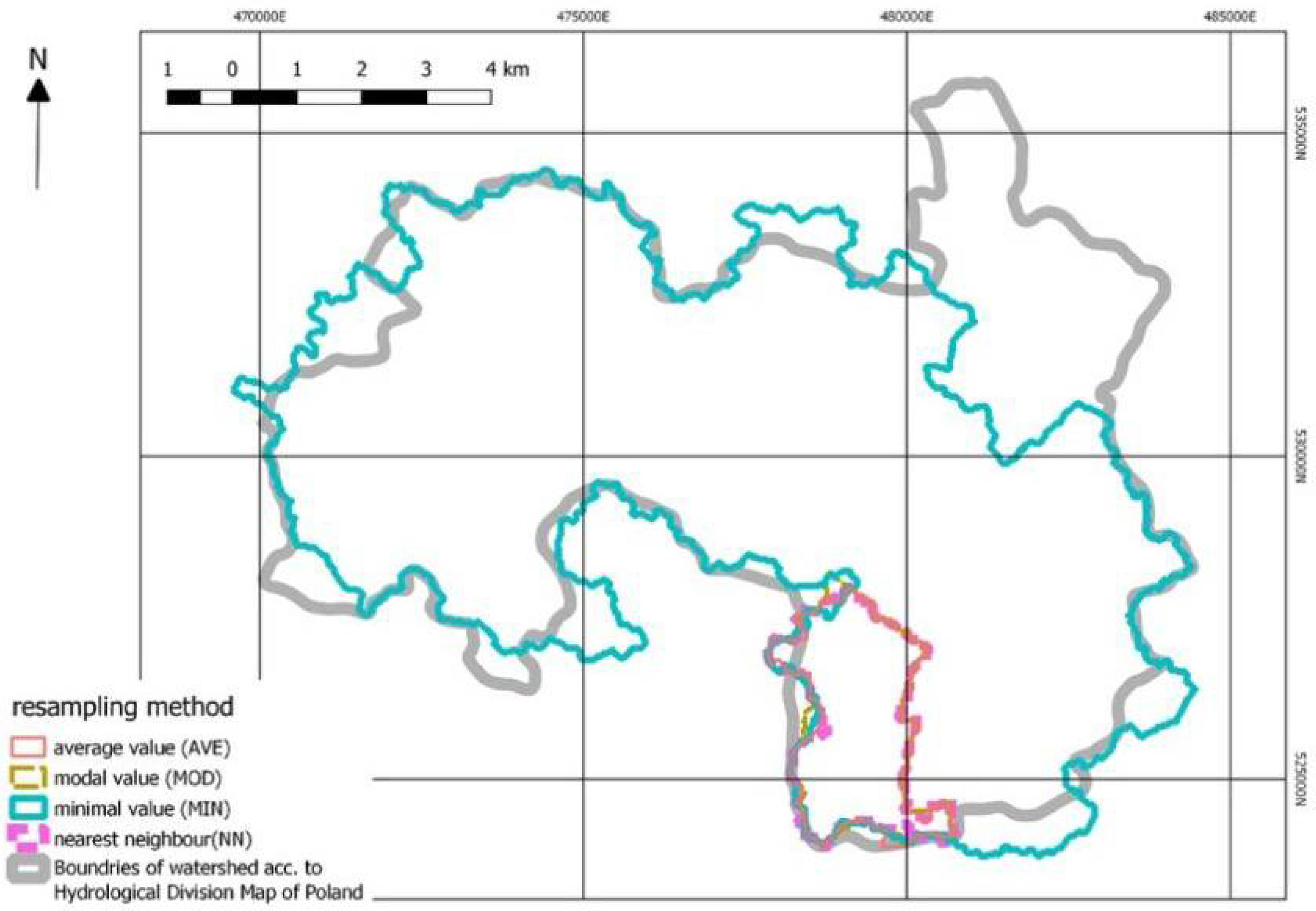
Figure 4.
Watersheds determined for DEM with a resolution of 26 m generated with the AVE, MOD, MIN, and NN methods on the background of watershed of the Hydrographic Division Map of Poland.
Figure 4.
Watersheds determined for DEM with a resolution of 26 m generated with the AVE, MOD, MIN, and NN methods on the background of watershed of the Hydrographic Division Map of Poland.
Figure 5.
Surface areas of determined watersheds for various DEM resolutions and resampling methods in comparison to the real area of the watershed (red line).
Figure 5.
Surface areas of determined watersheds for various DEM resolutions and resampling methods in comparison to the real area of the watershed (red line).
Figure 6.
Indicator of the normalized area error (NEA).
Figure 6.
Indicator of the normalized area error (NEA).
Figure 7.
Box plot chart of the dependence of the catchment area on the applied resampling method.
Figure 7.
Box plot chart of the dependence of the catchment area on the applied resampling method.
Figure 8.
Original maps with a resolution of 1 m with a section line (a) through the watercourse and (b) along the ridge.
Figure 8.
Original maps with a resolution of 1 m with a section line (a) through the watercourse and (b) along the ridge.
Figure 9.
Selection of 11 m resolution maps with a section line obtained by various resampling methods; (a) watercourse MIN 11 and (b) ridge MIN 11; (c) watercourse MED 11 and (d) ridge MED 11; (e) watercourse MAX 11 and (f) ridge MAX 11; (g) watercourse MOD 11 and (h) ridge MOD 11; (i) watercourse AVE 11 and (j) ridge AVE 11; (k) watercourse NN 11 and (l) ridge NN 11.
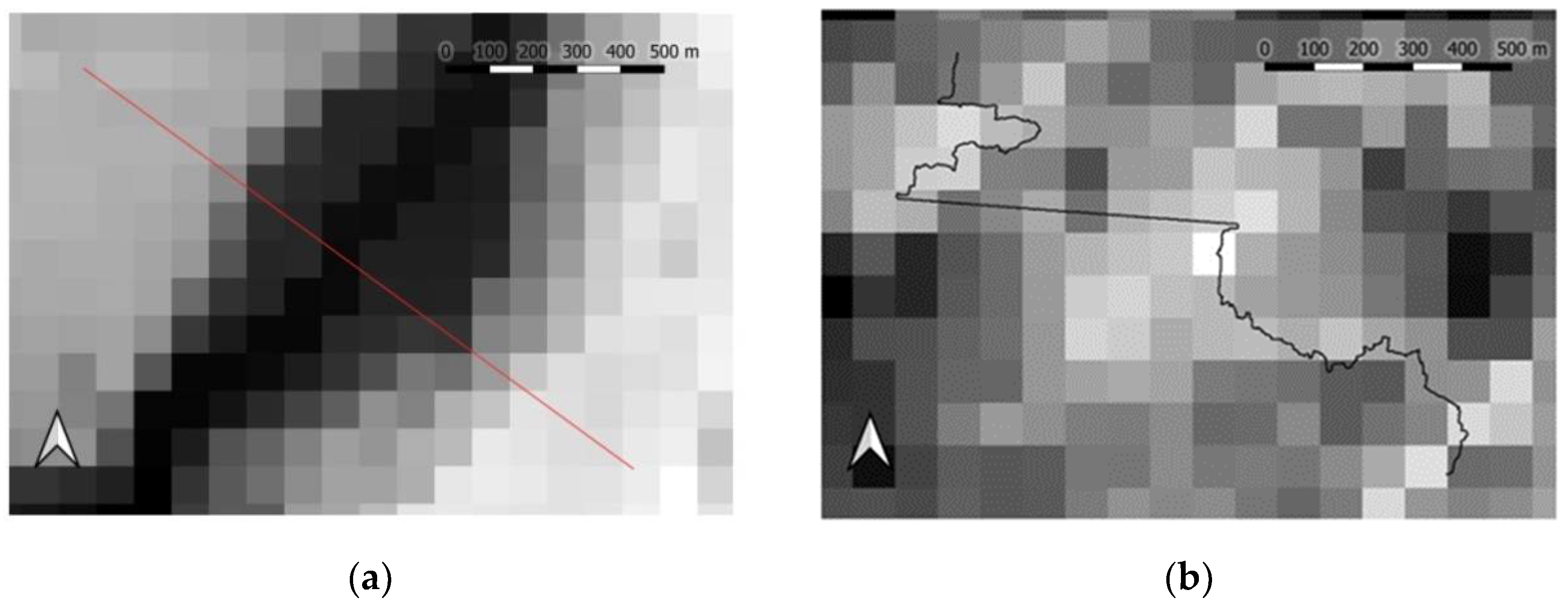
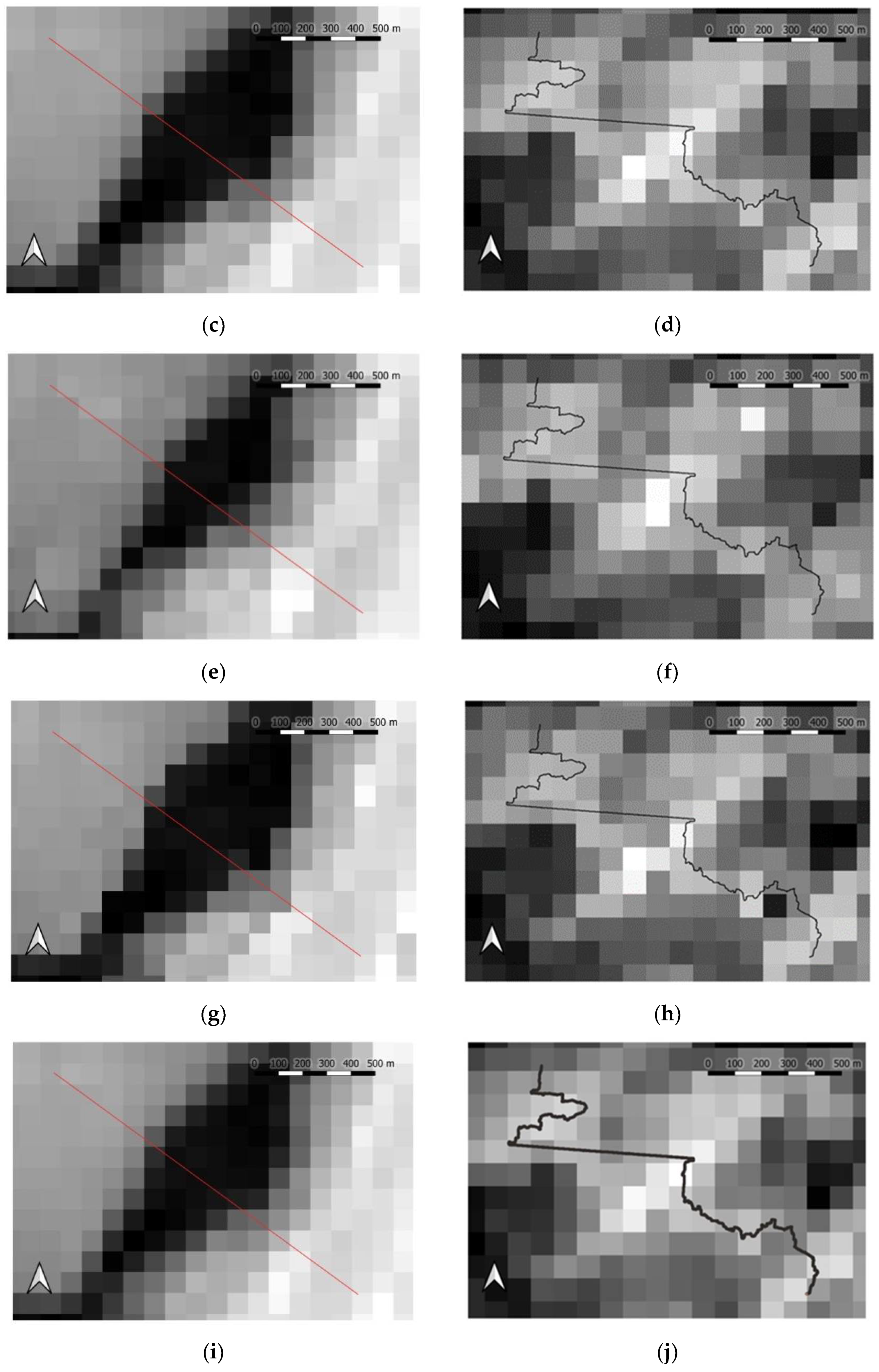
Figure 10.
Selection of 86 m resolution maps with a section line obtained by various resampling methods; (a) watercourse 86 and (b) ridge MIN 86; (c) watercourse MED 86 and (d) ridge MED 86; (e) watercourse MAX 86 and (f) ridge MAX 86; (g) watercourse MOD 86 and (h) ridge MOD 86; (i) watercourse AVE 86 and (j) ridge AVE 86; (k) watercourse NN 86 and (l) ridge NN 86.
Figure 11.
Cross-section along the ridge for all the resampling methods and sample resolutions of 11 m.
Figure 11.
Cross-section along the ridge for all the resampling methods and sample resolutions of 11 m.
Figure 12.
Cross-section along the ridge for all resampling methods and sample resolutions of 86 m.
Figure 12.
Cross-section along the ridge for all resampling methods and sample resolutions of 86 m.
Figure 13.
Indicator of the normalized area error for DEM resolutions from 1.5 to 7.6 m.
Figure 13.
Indicator of the normalized area error for DEM resolutions from 1.5 to 7.6 m.
Figure 14.
Difference between the area of the determined and referential watershed for DEM resolutions from 1.5 to 7.6 m.
Figure 14.
Difference between the area of the determined and referential watershed for DEM resolutions from 1.5 to 7.6 m.
Figure 15.
Comparison of the sum of lengths of the determined watercourses for DEM resolutions within 1.5 and 86 m for various resampling methods and the original DEM (red line).
Figure 15.
Comparison of the sum of lengths of the determined watercourses for DEM resolutions within 1.5 and 86 m for various resampling methods and the original DEM (red line).
Figure 16.
Comparison of average gradients of the determined watercourses for DEM resolution within 1.5 and 86 m for various resampling methods and original DEM (red line).
Figure 16.
Comparison of average gradients of the determined watercourses for DEM resolution within 1.5 and 86 m for various resampling methods and original DEM (red line).
Figure 17.
Cross-section of the watercourse for all resampling methods and sample resolutions of 11 m.
Figure 17.
Cross-section of the watercourse for all resampling methods and sample resolutions of 11 m.
Figure 18.
Cross-section of the watercourse for all resampling methods and sample resolutions of 86 m.
Figure 18.
Cross-section of the watercourse for all resampling methods and sample resolutions of 86 m.
Figure 19.
RMSE for DEM for all resolutions and resampling methods.
Figure 19.
RMSE for DEM for all resolutions and resampling methods.
Figure 20.
Changes of the surface area of a watershed along with the reduction in DEM resolution [
24,
43] (modified).
Figure 20.
Changes of the surface area of a watershed along with the reduction in DEM resolution [
24,
43] (modified).
Table 1.
Root mean square error (RMSE) for all generated DEMs.
Table 1.
Root mean square error (RMSE) for all generated DEMs.
| Method | Resolution [m] |
|---|
| 1.5 | 2.3 | 3.4 | 5.1 | 7.6 | 11 | 17 | 26 | 38 | 58 | 86 |
|---|
| AVE | 0.019 | 0.030 | 0.044 | 0.063 | 0.081 | 0.104 | 0.124 | 0.152 | 0.191 | 0.245 | 0.336 |
| MED | 0.019 | 0.030 | 0.043 | 0.059 | 0.080 | 0.108 | 0.136 | 0.161 | 0.193 | 0.245 | 0.332 |
| MOD | 0.032 | 0.049 | 0.062 | 0.086 | 0.088 | 0.129 | 0.164 | 0.182 | 0.214 | 0.280 | 0.361 |
| NN | 0.028 | 0.030 | 0.042 | 0.063 | 0.081 | 0.111 | 0.129 | 0.177 | 0.196 | 0.233 | 0.336 |
| MIN | 0.034 | 0.059 | 0.099 | 0.156 | 0.193 | 0.261 | 0.358 | 0.493 | 0.654 | 0.874 | 1.187 |
| MAX | 0.032 | 0.061 | 0.092 | 0.141 | 0.191 | 0.234 | 0.312 | 0.435 | 0.584 | 0.787 | 1.106 |
Table 2.
Resolutions and methods of watercourses for chosen resampling.
Table 2.
Resolutions and methods of watercourses for chosen resampling.
| Methods. Resolution [m] | Resampling Method |
|---|
| AVE | MIN | NN | MOD | MED | MAX |
|---|
| [km] |
|---|
| 1.5 | 48.3 | 47.0 | 47.5 | 47.0 | 48.4 | 48.1 |
| 2.3 | 46.6 | 46.7 | 46.6 | 42.5 | 46.6 | 42.3 |
| 3.4 | 46.7 | 47.5 | 45.9 | 47.2 | 45.4 | 41.2 |
| 5.1 | 47.3 | 45.1 | 43.7 | 47.8 | 42.3 | 43.5 |
| 7.6 | 47.2 | 36.1 | 39.0 | 45.9 | 43.3 | 43.7 |
| 11 | 43.7 | 36.0 | 54.4 | 38.2 | 45.7 | 1.9 |
| 17 | 38.9 | 36.2 | 44.9 | 1.8 | 40.8 | 1.9 |
| 26 | 2.0 | 35.1 | 1.9 | 1.8 | 2.0 | 1.7 |
| 38 | 1.9 | 37.9 | 1.8 | 1.9 | 1.8 | 1.8 |
| 58 | 1.7 | 37.6 | 1.8 | 1.8 | 2.0 | 1.2 |
| 86 | 1.8 | 36.5 | 1.7 | 1.6 | 1.7 | 1.6 |
Table 3.
Average gradients of watercourses for chosen resampling methods.
Table 3.
Average gradients of watercourses for chosen resampling methods.
| Resolution [m] | Resampling Method |
|---|
| AVE | MIN | NN | MOD | MED | MAX |
|---|
| [%] |
|---|
| 1.5 | 8.5 | 8.1 | 8.6 | 8.1 | 8.5 | 8.0 |
| 2.3 | 8.5 | 8.8 | 8.5 | 8.6 | 8.7 | 8.0 |
| 3.4 | 8.0 | 8.4 | 8.3 | 8.2 | 8.8 | 7.0 |
| 5.1 | 7.9 | 7.6 | 8.1 | 7.4 | 8.0 | 6.9 |
| 7.6 | 7.7 | 7.8 | 7.3 | 6.8 | 7.3 | 6.1 |
| 11 | 7.1 | 7.9 | 6.1 | 6.1 | 6.8 | 0.0 |
| 17 | 6.4 | 8.3 | 5.9 | 0.0 | 6.3 | 0.0 |
| 26 | 0.0 | 8.7 | 0.0 | 0.0 | 0.0 | 0.0 |
| 38 | 0.0 | 8.2 | 0.0 | 0.0 | 0.0 | 0.0 |
| 58 | 0.0 | 8.6 | 0.0 | 0.0 | 0.0 | 0.0 |
| 86 | 0.0 | 8.1 | 0.0 | 0.0 | 0.0 | 0.0 |
Table 4.
Comparison of RMSE obtained in this research and those obtained in another studies.
Table 4.
Comparison of RMSE obtained in this research and those obtained in another studies.
| Degree of Change | Change in Resolution [m] | RMSE [%] |
|---|
| Haile and Rientjes [23] | This Studies | Haile and Rientjes [23] | This Studies |
|---|
| 3x | from 1.5 to 4.5 | from 1 to 2.3 | 3.13 | 2.98 |
| 5x | from 1.5 to 7.5 | from 1 to 5.1 | 3.54 | 6.29 |
| 7x | from 1.5 to 10 | from 1 to 7.6 | 2.81 | 8.12 |
| Publisher’s Note: MDPI stays neutral with regard to jurisdictional claims in published maps and institutional affiliations. |
© 2022 by the authors. Licensee MDPI, Basel, Switzerland. This article is an open access article distributed under the terms and conditions of the Creative Commons Attribution (CC BY) license (https://creativecommons.org/licenses/by/4.0/).


