Article

Effects of Land Use/Cover on Regional Habitat Quality under Different Geomorphic Types Based on InVEST Model

1
State Key Laboratory of Resources and Environmental Information System, Institute of Geographic Sciences and Natural Resources Research, Chinese Academy of Sciences, Beijing 100101, China
2
University of Chinese Academy of Sciences, Beijing 100049, China
3
Jiangsu Center for Collaborative Innovation in Geographical Information Resource Development and Application, Nanjing 210023, China
4
Collaborative Innovation Center of South China Sea Studies, Nanjing 210093, China
*
Author to whom correspondence should be addressed.
Remote Sens. 2022, 14(5), 1279; https://doi.org/10.3390/rs14051279
Submission received: 20 December 2021 / Revised: 22 January 2022 / Accepted: 3 March 2022 / Published: 5 March 2022
(This article belongs to the Special Issue Remote Sensing and GIS for Geomorphological Mapping)

Abstract

:
Research on habitat quality change is of great significance for regional ecological security. Analysis of spatiotemporal change of habitat quality based on different geomorphic types can restore the background of ecological environment in historical periods and provide scientific support for revealing the evolution law of regional ecological environment quality and ecological restoration. This study aimed to identify the change in habitat quality under different geomorphic types from 1995 to 2018. Based on DEM data, geomorphic types of different scales were divided. The InVEST habitat quality model was used to analyze the spatiotemporal change in habitat quality in individual land use types in the Altay region. The spatiotemporal changes and main influencing factors of habitat quality under the background of different geomorphic types were explored. Remote sensing data was used to analyze the land use/cover changes. Sixteen threat sources, their maximum distance of impact, mode of decay, and sensitivity to threats were also estimated for each land use type. The results showed that habitat quality decreased significantly in 2015, which was related to the rapid expansion of cultivated and construction land as threat sources, as well as the decrease of forestland and grassland as sensitive factors. However, habitat quality improved significantly in 2018, because of the implementation of ecological restoration policy in 2015. Affected by elevation and topographic relief, the geomorphic type with the best habitat quality index was the large undulating middle mountain (0.927) and the worst was the medium altitude platform (0.351). Woodland contributed the most to habitat quality in large undulating middle mountain (35.07), and bare rock gravel land contributed the most to medium altitude platform (127.68). Habitat quality of different geomorphic types showed obvious spatial aggregation, and from high altitude to low altitude showed a banded ladder-like distribution. Changes in habitat quality during the past three decades suggested that the conservation and restoration strategies applied in regional ecosystem were effective. On the basis of the analysis results, four types of zoning management schemes were divided, and the ecological management and conservation measures were put forward. Therefore, this study can help decision makers, especially regarding the lack of data on biodiversity.

1. Introduction

The contribution of biodiversity to the global economy, human survival, and welfare has increased recently [1,2]. With the strengthening of human activities, the interference to the ecological environment is increasing, which seriously affects and changes the status of ecologic environment and disturbs the quality of biological habitat (i.e., habitat quality) [1,3,4]. Therefore, the decline in biodiversity is higher than in the past and is expected to rise in the future [5,6]. This brings great challenges to the protection of biodiversity. Biodiversity includes the diversity of animals, plants, and microorganisms at the genetic, species, and ecosystem levels, and it provides regulation and support for ecosystem services [7,8]. Habitat quality refers to the ability of the ecosystem to provide suitable conditions for the sustainable development and survival of individuals and populations, and it reflects the status of regional biodiversity and ecosystem health to a certain extent, and plays an important role in maintaining biodiversity [9,10]. Land-use dynamics is one of the main activities of human beings to transform the natural environment and interfere with habitat quality. Its degree of change reflects the intensity of human activities. Land-use change has become one of the important risk factors affecting the quality of natural environment and biological habitat [11]. In particular, the expansion of urban construction land and agricultural land will aggravate the destruction of natural environment and biological habitat and hinder the connectivity of habitat [12], thereby aggravating the fragmentation and degradation of habitat and even leading to the disappearance of habitats [13].
Habitat quality is the ability of an ecosystem to provide all necessary goods and services in sufficient quantity for all its living environments [14]. It represents the overall ecological quality based on the spatial distances between habitat quality and the threats caused by human activities, which can be weighted to consider their impacts [3,15]. That is, habitat quality is the quality of natural resources closely related to human beings, and it is also the quality of the human living environment, including natural resources and various elements of the entire environment [16]. With the rapid development of the world population and social economy, people’s demand for land resources is increasing, and changes in the intensity and ways of land use have severely damaged the ecosystem, leading to the reduction and degradation of ecosystem service capabilities in many areas [17]. Therefore, studying the relationship between land use changes and habitat quality changes can provide a basis for analyzing regional ecological environment changes, formulating regional ecological protection policies and achieving the sustainable use of land resources [18].
Currently, habitat quality assessment methods can be divided into two categories. One method involves obtaining habitat quality parameters through field surveys. This method investigates field samples, and on this basis, a comprehensive evaluation index is built to evaluate the habitat quality. For example, Liu investigated the biodiversity and evaluated habitat quality of West Lake Nature Reserve [19]. Liu et al., conducted an investigation and analysis of the habitat quality of rivers in Yixing section of Taihu Lake Basin [20], and Yang et al., investigated the habitat quality of Laizhou Bay [21]. However, the field survey sampling method tends to focus on small geographic areas or single species habitats, and this method is limited by time and manpower requirements, making it difficult to conduct long-term data analysis. The second method involves using models to evaluate the habitat quality. Some common evaluation models include InVEST model (Integrated Valuation of Ecosystem Services and Trade-offs), but it should set different parameters according to different research areas [22,23]; SoLVES model (Social Values for Ecosystem Services), but the questionnaire in SoLVES model involves the understanding of different respondents [24]; SDMs(Species Distribution Models), but SDMs models need to clarify interactions between species [25,26], and other models. Although there are some limitations in using digital model evaluation, compared with the method of field data measurement, using model evaluation has obvious advantages, as its operation is simple and fast and there is no need for field measurement to obtain data, so it is widely used. Domestic and foreign scholars mostly use the InVEST model with simple operation, convenient data access and fewer parameters to conduct multi-scale quantitative habitat quality assessment and express the analysis results in the form of a thematic map [12,27,28,29]. InVEST model is widely used because of its low demand for data, strong spatial visualization, and high evaluation accuracy of its calculation results, and can reflect the habitat distribution under different landscape patterns. The habitat quality module of the InVEST model evaluates habitat quality by analyzing land use/cover (LULC) maps and the threat degrees of different land use types to biodiversity. This model evaluates the biodiversity status in the landscape and uses LULC changes and biodiversity threat data combined with expert knowledge to obtain the consistent indicators of biodiversity responses to the threats [3,30]. According to the relative ranges and degradation degrees of different habitat types, the habitat quality determined by the InVEST model has been successfully used to maintain biodiversity. As a few recent examples, Aneseyee et al. [31] used the InVEST habitat quality model associated with LULC changes to conduct a qualitative case study of the Winike Watershed, and found that the ranges of agro-ecology facilitate a diversity of plants, wild animals, and birds in the area. Polasky et al., evaluated the impact of actual land-use change and a suite of alternative land-use change scenarios, and demonstrated that while large-scale agricultural expansion increased landowners’ income, it resulted in significant losses of stored carbon and negative impacts on water quality, resulting in a decline in general terrestrial biodiversity and habitat quality for forest songbirds [28]. Gong et al., evaluated the changes in plant biodiversity in a mountainous area in the Bailong River Basin in Gansu Province, and found that the higher habitat quality area mainly distributed in the nature reserve and forest, which could provide a good living environment for more endangered plant and animal species [32]. Mushet et al., analyzed the characteristics and changing trends of amphibious habitats of various land use types, and showed that wetland drainage and grassland conversion, an economic climate favoring commodity production over conservation, have destroyed a large amount of amphibian habitats and will likely continue into the future, which will reduce the number of amphibians [33]. The changes in the Boye wetland of Jimma, Ethiopia, reduced the avifauna population and species composition [34]. Sallustio et al. [30] and Terrado et al. [3] assessed habitat quality in Italian nature reserves and watersheds under different nature conservation planning scenarios using the InVEST model. Du and Rong used the two indicators of Habitat Quality Index and Habitat Degradation Index to represent the function of biodiversity and analyzed the impact of land use changes on biodiversity in Shanxi Province [35]. Chen et al., calculated the impacts of background threat sources on habitat quality degradation using this model and analyzed the impact of land use changes on habitat quality changes [36]. Liu and Xu compared the spatial-temporal evolution of habitat quality between Xinjiang Corps region and Non-corps region based on land use with the InVEST model, and predicted the trend of habitat quality from 2018 to 2035 [37]. Using the InVEST model, many researchers have investigated the impact of land use changes on habitat quality.
The earth’s surface morphology (physiognomy) is the carrier of biological survival, human production, and life. Due to the action of internal and external forces, the difference of development stages and geological movement, the earth’s surface formed different altitudes and fluctuation patterns, which will affect the regional material migration and the redistribution of hydrothermal conditions [38]. Physiognomy also directly affects the surface vegetation and land use through altitude, surface relief state, and denudation degree [39,40,41]. Therefore, physiognomy is the foundation of land use spatial patterns. A geomorphic entity divided according to the same or similar characteristics is a geomorphic type, that is, the geomorphic unit whose geomorphic form, genesis, and development process are basically consistent [42]. In different studies, different scholars will choose dominant factors to divide geomorphic type according to their research purpose. Physiognomy is a comprehensive entity including basic elements such as altitude, slope, slope direction, genesis, and material composition. It is an important environmental condition affecting biological habitat and human activities, and physiognomy has a great impact on the ecosystem. Especially in mountainous areas with large topographic relief, the ecosystem will be relatively fragile, which will not only affect the ecosystem services but also hinder the regional sustainable development. However, the current research on land use and habitat quality only considers one or several topographic factors, and research on land use and habitat quality under different geomorphic types has not been carried out. On the premise of dividing geomorphic types, doing the research has important theoretical reference and practical significance for balancing and coordinating regional ecological protection and development. Therefore, this paper took the Altay region with diverse geomorphic types and complex ecosystems as a study area. The area has diverse topographic features, including flat land, hills, plains, gorges, and steep slopes. Especially in mountainous and hilly areas, physiognomy redistributes temperature, water, light, and then changes the land use form and intensity, and ultimately affects the quality of habitat. Therefore, it is incomplete to simply select one or several topographic factors to study the impact of land use change on habitat quality. Under the background of different geomorphic types, researching land use types and habitat quality is more scientific and complete. Analyzing habitat quality based on different scale geomorphic types is helpful to understand the heterogeneity of biological habitat comprehensively and objectively. The Altay region, known as “Golden Mountain and Silver Water”, is rich in mineral and energy resources. Grassland and forest areas are relatively large, making it one of the six major forest areas in China and also an important green protection and ecological safety zone. There are 30 national and autonomous nature reserves in the Altay region. Nature reserves are important areas for biodiversity conservation. Furthermore, nature reserves also play a vital role in purifying air, water conservation, regulating climate, and reducing soil erosion. However, in recent years, with the serious overgrazing, over reclamation, and unreasonable use of natural resources, the quality of ecological environment in the Altay region has been declining. Various problems appear, such as bare ground, shrinking wetland areas, reduction of animal and plant populations, degradation of dominant species, and serious imbalance of ecological carrying capacity. These threats result in the degradation of the habitat and biodiversity and have a serious impact on the production and life of residents. Therefore, the objective of this study is to (1) map and identify habitat quality of different geomorphic types and analyze the spatiotemporal changes of habitat quality from 1995 to 2018 and (2) explore the correlation between land use types and habitat quality under the background of different geomorphic types in the Altay region. On this basis, combined with decision support systems, it can help users with rational planning and use land to protect the environment [43,44].

2. Materials and Methods

2.1. Study Area

The Altay region is located in the hinterland of Eurasia and north of Xinjiang, China, with a geographic scope of 85°31′~91°01′E, 45°00′~49°10′N (Figure 1). The region has a high latitude, great vertical climate differences, and a significant local microclimate. It belongs to the temperate continental cold climate. The region borders Mongolia, Kazakhstan, and Russia. It is 402 km from east to west and 464 km from north to south, with a total area of 1.18 × 10⁵ km², accounting for 7.2% of the total area of Xinjiang. The region governs six counties and one city, all of which are border counties (cities), and it is a multi-ethnic area composed of 39 nationalities. By the end of 2020, the total population of the region was 668,587.
There are various geomorphic types in this area, including three large geomorphic units: plain area, mountainous area, and desert (Gobi) area. The Altay region includes the Altai Mountains in the north, Shawuer Mountains in the west and Junggar Basin in the south. The central region is the south of the Irtysh valley. The area south of the Ulungur River is part of the hilly plain on the northern edge of the Junggar Basin and the Gurbantunggut Desert. The terrain of the mountains area is high in the west and low in the east, showing an obvious ladder shape, while the hilly-plain region is the opposite. The mountain area accounts for about 32% of the total area, with the lowest altitude of 317 m and the highest altitude of 4374 m. It is one of the focus areas of cross-border water security issues of international concern with three major surface runoff sources: the Irtysh River, the Ulungur River, and small rivers in Jimunai County. The ecosystems in this area are diverse. Glacier, forest, grassland, wetland, desert, farmland, and other ecosystem types are distributed, which form a complete “mountain-river-forest-field-lake-grass life community” [45]. There are various types of soil, including mountain soil and plain soil, as well as saline soil, swamp soil, and cracked soil. However, under the influence of human factors such as long-term development of mineral resources [46], grassland overgrazing, and oasis agricultural overdevelopment [47], coupled with the superposition of natural factors such as fragile ecosystems, climate change, and the decline of groundwater level in arid areas, the study area is faced with increased soil erosion, forest and grassland degradation, decreased ecosystem connectivity, habitat fragmentation, reduced water conservation function and biodiversity function, and other prominent problems. The ecosystem health and ecological security in the study area are facing great challenges [48].

2.2. Data Preparation

This paper used remote sensing data to interpret land use/cover types. Finally, we got land use classification data in 1995, 2000, 2005, 2010, 2015, and 2018. We used remote sensing images with a 2 m resolution from the Gaofen-1 satellite (GF-1) (http://36.112.130.153:7777/DSSPlatform/productSearch.html, accessed on 21 March 2019). To improve the accuracy of visual interpretation, the image selection was mainly based on remote sensing data from June to September (during the vegetation growing period) of the current year or adjacent years, and the cloud cover of images was less than 10%. To eliminate the influence of atmosphere, temperature, Earth rotation, sensors and other factors on image deformation in the imaging process, cloud shadow detection, and geometric and radiometric correction were carried out for all images [49]. Then, the remote sensing image of the study area was obtained by orthophoto correction fusion, image registration, stitching, and mask cutting. Envi 5.3, Locspace viewer (LSV) and ArcMap 10.6 software were adopted. Combined with supervised classification and manual visual interpretation, various land use/cover data were extracted [50,51,52]. Among them, land use type classification was based on the Chinese land use classification system issued by the Chinese Academy of Sciences (https://www.resdc.cn/, accessed on 13 July 2021). According to the land cover characteristics and land use optimization, the grid database of land use types in the study area was obtained. The results of supervised classification contained some sporadic points that were inconsistent with the actual situation. To improve the interpretation accuracy, Google images was used for manual visual interpretation of land use classification. Therefore, the land use in 2019 was revised again (Table 1) and used as a benchmark. The remaining images were interpreted and corrected by superimposing remote sensing images and Google images. The comprehensive accuracy of the first class of land use types in these six periods is more than 94.3%, and the second class is more than 91.2%. In order to ensure the quality of data interpretation, we conducted field surveys in the study area and obtained a large number of field survey records and photos. In 2018, the accuracy rate of identifying cultivated land reached 99%, the grassland, forestland, and construction land reached 98%, and the comprehensive accuracy was over 95%. From the perspective of single land type, the accuracy of cultivated land was the highest, above 97% in all six periods. The main reason for the misclassification was that individual cultivated land distributed in the forestland was mistakenly classified as forestland and some unused land with regular and sparse vegetation was misclassified as cultivated land. The accuracy of grassland was above 96%, mainly because some sporadic grasslands were misclassified as cultivated land or low forestland. The accuracy of construction land was more than 95%, because the spectral information of some large plant roofs was close to bare land, which was wrongly divided into unused land. The accuracy of water was 99%, because some small ponds were submerged in other land types. The unused land in the Altay region includes sandy land, Gobi, saline alkali land, swamp, bare land, and bare rock gravel land, with a classification accuracy of 94%, mainly because some sandbars with sporadic vegetation were mistakenly divided into cultivated land, and the interlaced beach of water was mistakenly divided into construction land.
In this paper, SRTM_DEM data with 30 m resolution was selected; neighborhood analysis method and mean change point analysis method were used to determine the best statistical unit of fluctuation in the study area [53,54,55]. Consulting the achievement data of 1:1 million geomorphic types in China (https://www.resdc.cn/Default.aspx, accessed on 13 July 2021), the basic geomorphic types of the Altay region were divided.

2.3. Methods

2.3.1. Classification of Geomorphic Types

Physiognomy directly affects the distribution of surface vegetation and land use through altitude, fluctuation, and denudation degree. Consulting the previously published classification schemes of geomorphic type at all levels and all scales throughout the country and the latest 1:1 million digital geomorphic classification method, a geomorphic classification method that used continuous polygon patches and discrete point, line, and surface patches to jointly reflect the causes and structural types of geomorphic morphology is formed [56,57]. In addition, the classification of geomorphic types based on the description of geomorphic morphological characteristics by topographic factors is gradually developing [39,40,41]. In this paper, DEM data were used to divide geomorphic types with the help of a multiscale segmentation algorithm and topographic factors [58,59].
To make the land type classification system more scalable, this study followed the “China land 1:1 million digital geomorphic classification system” [55,60] and took altitude and surface relief as the most important factors for geomorphic type classification. On this basis, the classification standards of geomorphic types were adjusted in combination with the actual geomorphic characteristics of the study area. Finally, the classification system of Table 2 was obtained.
In the existing research, reliable results have been achieved in the application of DEM segmentation based on a multiscale segmentation algorithm [41,61]. It was found that the boundaries of different geomorphic types were mostly areas with great changes in slope [62], so in this study, altitude, surface fluctuation, and slope change rate reflecting the geomorphic boundaries were selected as the division indexes of geomorphic types (Table 3). The multiscale segmentation algorithm and the classification criteria in Table 2 were used to divide the geomorphic type.
For surface relief, the research showed that the value of relief presented an inverted “U” shape with the change in neighborhood area, also known as logarithmic curve [41,53,54,63], where the curve changes from steepness to slowness represent the size of the optimal statistical unit. The most commonly used method to find the turning point is based on the mean change point method. Therefore, this paper used the 30 m resolution SRTM_DEM data, neighborhood analysis method, and mean change point analysis method to determine the best statistical unit of fluctuation in the study area.
The mean change point method is a mathematical statistical method for processing nonlinear data. This method is the most effective for a test with exactly one change point [64]. Using this method must meet the logarithmic curve. The only point at which the curve changes from steepness to slowness is the size of the optimal statistical unit. The change point is calculated as follows:
Assume (Xt, t = 1, 2, …, N). Let i = 2,…, N, divide the sample into two segments for each i: x 1 , x 2 , …,   x i 1 and x i , x i + 1 , …, x N . Calculate the arithmetic mean of each sample X i 1 , X i 2 and the statistics of S and S i . The existence of a change point will increase the difference between S and S i to find the best statistical unit:
S i = t = 1 i 1 ( x t X i 1 ¯ ) 2 + t = i N ( x t X i 2 ¯ ) 2
X ¯ = t = 1 N x t N   and   S = t = i N ( x t x ¯ ) 2
According to the theory of topographic relief and the theory of geomorphic development stability, there must be a unique point where the change rate of the height difference changes sharply. To find this point accurately, we used the mean change point analysis method to scientifically analyze the resulting data.
First, the data were processed to calculate the surface relief T per unit area, which was obtained by the following formula:
T i = t i s i   ( i = 2 ,   3 ,   4 ,   ,   30 )
where t i represents the surface relief under the analysis window, s i represents the grid cell area under the analysis window, and T i is the unit surface relief under the analysis window.
Second, take the logarithm ln ( T )   of T to obtain sequence X ( x i ,   i = 1, 2, 3, …,30).
Finally, the data were processed according to Equations (1) and (2) to obtain the calculation statistics S and S i . Because the existence of change point increases the gap between S and S i , the best statistical window is derived by the change point analysis method.

2.3.2. The Invest Habitat Quality Model

An open-source InVEST model of habitat quality version 3.8.0 (https://www.naturalcapitalproject.org/invest/, accessed on 07 December 2021) has been developed recently at Stanford University by Sharp et al. [22] to map and assess the habitat quality for individual LULC types. The InVEST habitat quality model is a novel tool used for assessing habitat quality under anthropogenic threats [30,65]. The key reason for using this model is: (1) Compared with other models, this model is relatively less data-intensive and more flexible; (2) it can be easily adapted to a specific context and readily available global or local data [12]; (3) the model shows the hydrological and ecological connectivity developed by vigiak et al. [66] and its applicability to regional scale. More importantly, the InVEST habitat quality model is unique in its ability to analyze spatial habitat quality trends and connectivity for each land use type and quantify sensitivity to threats.
This paper used the habitat quality module in the InVEST model to evaluate the habitat quality. The InVEST habitat quality model can reflect biodiversity by evaluating the range of various habitat quality types or vegetation types and the degradation degree of each type. The main principle is to combine the sensitivity of various landscape types in the assessment area and the intensity of landscape threat factors to obtain the distribution of habitat quality. Habitat quality is closely related to land use changes. Human use of land changes the type of land use and affects the level of habitat quality. The greater the intensity of human activities, the greater the threat to the regional habitat quality, and the lower the level of habitat quality and biodiversity [67,68].
For modeling the habitat quality, different geospatial data parameters were prepared using ArcMAP 10.6 (Table 4). Based on Sharp et al. [22] and other researches [6,30,69,70,71], used data on LULC, the relative weight of each threat ( ω r ), the habitat sensitivity of each threat ( S j r ), the longest distance between habitats and sources of threats ( d r m a x ), and habitat suitability ( H j ) to model habitat quality. These parameters were determined by expert knowledge supported by field investigations [3] and previous research results.
The degree of habitat quality is represented by the Habitat Quality Index. Habitat quality is based on the availability of living resources, the amount of reproduction and presence of organisms, and the ability of an ecosystem to provide suitable living conditions for individuals and populations. Its value is between 0 and 1, and the higher the value, the better the habitat quality. In other words, the assessment by this module reflects the influences of human activities on the eco-environment. The stronger the intensity of human activities, the greater the threat to the habitat and the lower the habitat quality and the biodiversity level in this region; on the contrary, the higher the habitat quality, the lower the interferences from human activities and the higher the biodiversity level in this region [72]. This paper combines the sensitivity of different land use types to threat factors and the intensity of the external threats to calculate the habitat quality of the study area, thereby reflecting the suitability of the combination of human survival and sustainable development of the social economy [31]. The specific calculation formula is as follows:
Q x j = H j [ 1 ( D x j z D x j z + k z ) ]
where Qxj is the habitat quality of grid x in land use type j; Hj is the habitat suitability of land use type j; Dxj is the habitat degradation degree of grid x in land use type j; k is the half-saturation constant; z is the normalization constant, and usually takes the value 2.5, and the calculation formula of Dxj is as follows:
D x j = r = 1 R y = 1 Y r ( ω r r = 1 R ω r ) r y i r x y β x S j r
where r is the threat source; R is the number of threat sources; y is the grid number of threat source r; x is the number of grids in the habitat; Yr is the number of grids occupied by threat sources; ωr is the weight of the threat source r, which represents the relative destructive power of a certain threat factor to all habitats, with a value range of 0–1; irxy is the threat level of the threat source value ry of the grid y to the habitat grid x; βx is the accessibility level of grid x, with a value range of 0–1, the larger the value, the easier it is to reach; and Sjr is the sensitivity of land use type j to threat source r, with a value ranging from 0 to 1, and the larger the value, the more sensitive. The model provides both linear and exponential recession calculation methods for the calculation of irxy:
i r x y = 1 ( d x y d r max )   ( if   it   is   linear   decay )
i r x y = exp [ ( 2.99 d r max ) d x y ]   ( if   it   is   exponential   decay )
where dxy is the distance between grid x and grid y; and drmax is the influencing scope of the threat factor r.
The systematic random sampling method [74] was used to conduct a sampling survey on six counties and one city under the jurisdiction of the Altay region. To this end, 24 experts from the office of environmental protection and natural resources (2 experts from each county/city, who have a good understanding of the ecology) were interviewed. The survey was designed according to the method of Diehl et al. [75] to better understand people’s views on the importance of specific threats. The respondents were asked to identify the habitat types, as well as the major threats found in the area: expansion of cultivated land, urban and rural construction, industrial and mining land, unused land, etc. The 24 experts also responded to the causes of habitat degradation, the maximum distance of the threat affects the habitat quality, the propagation speed of the threat (distance attenuation measurement), sensitivity measurement (which threat has a greater impact on the habitat), the overall situation of the habitat quality in the area, and the measures adopted so far to control the threat to the ecosystem in the study area. Next, opinions regarding the major threats’ impact on specific land use types (paddy land, dry land, woodland, shrub wood, sparse wood, other woodland, high coverage grassland, medium coverage grassland, low coverage grassland, Canal, Lake, pit-pound, urban land, rural residential land, industrial and mining land, unused land) were explored using the analytical hierarchy process (APH) model. APH model is widely used to assign a weight to each threat by examining the potential impact of each threat on habitat using a pairwise comparison matrix [76]. By using expert-based judgment, a matrix was established for each county/City, including threats for pairwise comparison. Divide the weight of each element provided by experts in the matrix by its total number of columns to generate a standardized pairwise matrix. Finally, use the eigenvectors (priority vectors) to generate a weighted matrix (average the rows of the matrix) that shows the impact of each factor on the habitat [77]. Verify that the consistency ratio (CR) of acceptable accuracy for pairwise comparisons in the judgment matrix is less than 10% [76]. Finally, the average threat weight/sensitivity values for the county/city were used for each land use type.
To sum up, starting from the impact of land use change on habitat quality, comprehensively considering the current situation of the study area, relevant research results, and local expert opinions, three kinds of anthropogenic threats were identified in the region by following the approach of Terrado et al. [3]. They were agricultural expansion, construction land increase, and unused land. The reason is that cultivated land and construction land are the main places for human production and life, which have a great impact on the ecological environment. The unused land in the study area is mainly desert, Gobi, bare land, bare rock gravel, etc. The natural background conditions are poor, the vegetation coverage is low, and the environmental conditions are harsh. If reclamation is arbitrary, land desertification, salinization, and desertification will be caused, and the habitat quality will be reduced to varying degrees. Affected by the distribution of surface water, the cultivated land is subdivided into paddy land and dryland. In addition, considering that there are many mountains, hills, and deserts in the study area, rural settlements are scattered, and due to the rich mineral resources in the Altay region, the industrial and mining land is widely distributed, so the construction land is refined into urban land, rural residential land, and industrial and mining land (Table 5).
The relative habitat suitability score (intensity of the threat) can be assigned to each LULC type, ranging from 0 to 1, where 1 indicates the highest habitat suitability and 0 indicates the lowest suitability [22,23,28], and in combination with previous research results [29,35,36,37,67,73,78,79] and expert opinions, we finally obtained the corresponding parameter settings (Table 6).

2.3.3. Hotspot Analysis and Spatial Data Exploration of Habitat Quality

Spatial autocorrelation refers to the correlation of a variable in different spatial positions, which indicates the aggregation degree of attribute values of spatial units. Commonly used autocorrelation indicators include global Moran’s I index and Getis-Ord G* coefficient. A large number of simulation calculations show that Moran’s I can find out whether the data is clustered in general, while the Getis-Ord G* coefficient more specifically indicates whether there are clusters of high/low values [80,81,82,83]. To accurately reflect the spatial aggregation of habitat quality, this paper combines the two indicators [83]. The global Moran’s I index is used to describe whether the habitat quality in the study area has a regional agglomeration effect. Its value range is [–1, 1]. If the index is greater than 0, it is a positive correlation, indicating that similar attributes are clustered together, and the closer the value is to 1, the higher the degree of clustering. Otherwise, it is a negative correlation, indicating that different attributes are clustered together, and the closer the value is to −1, the higher the agglomeration degree. If the index is equal to 0, it indicates random distribution or no spatial autocorrelation. The calculation formula is as follows [84]:
I = i = 1 n j = 1 n W i j ( x i x ¯ ) ( x j x ¯ ) S 2 · i = 1 n j = 1 n W i j
s 2 = 1 n · i = 1 n ( x i x ¯ ) 2
where n represents the total number of regional spatial units, that is, the number of geomorphic type units divided in this study. x i and x j represents the attribute value of random variable x on geographical units i and j , that is, the habitat quality value on different geomorphic types of units i and j . x ¯ is the average attribute values of n spatial geographical units. W i j is the weight matrix of the adjacency relationship between spatial geographical units. Therefore, if zone j is adjacent to zone i, the product receives a weight of 1, otherwise, the product receives a weight of 0. A study generalized these definitions to include any type of weight, and in a wider term, W i j is a distance-based weight which is the inverse distance between locations i and j(1/ d i j ). In this paper, the length between centroids is used to calculate.
Based on Moran’s I index, Getis-Ord G* is used to describe the cold and hot spots of habitat quality in the study area to analyze the agglomeration of habitat quality in local space. When the G* value is significantly positive, the habitat quality shows high value agglomeration, which is a hot spot area, on the contrary, it is a cold spot area. Among them, the regions corresponding to the G* value at the 99% confidence level are hot and cold spots, and at the 95% confidence level are sub hot spots and sub cold spots. The calculation formula is as follows [85]:
G i * = j n w i j x j x ¯ j = 1 n w i j S [ j = 1 n w i j n j = 1 n w i j ] 2 n 1
where x j is the habitat quality of geomorphic type unit j . w i j is the spatial weight matrix of geomorphic type units i and j (calculated by Queen contiguity). The two most commonly used spatial matrices are adjacent matrix and inverse distance matrix. In this paper, a weight matrix based on adjacency relationship was used. Among them, the queen weight matrix with better detection results, in its definition, as long as there is a common edge or the same point between two spatial objects, it is considered that they are adjacent, and the weight is 1, otherwise the weight is 0 [80,86]. x ¯ is the average value of habitat quality. S is the standard deviation of habitat quality. n is the total number of geomorphic type units divided.
Within different geomorphic type units, take the second-class land use types in Table 1 as the impact factors to explore the impact of land use types on habitat quality. Index contribution indicates the contribution of an index to habitat quality, and its value can reflect the factors leading to the difference in habitat quality. Therefore, different land use types are used as impact indicators to calculate the factors’ contribution to habitat quality. The calculation formula is as follows:
C i x = w i C H i x Q x × 100 %
where i and x represent land use type and geomorphic type, respectively. C i x represents the contribution of i to the habitat quality of x . C H i x represents the ratio of i ’s pixels to x ’s pixels. Q x is the habitat quality of geomorphic type x . w i represents the weight of land use type i , which is represented by the habitat suitability index in Table 5. Habitat suitability scores were determined based on literature data and experts’ knowledge [22,23,28], which had certain subjectivity and objectivity, so that it cannot only take into account the subjective preference of decision makers, but also reduce the subjective randomness of empowerment [87]. In addition, different geomorphic types included different land use types, the proportion of each land use type was different, and the habitat suitability of different land use types was also very different. The InVEST model believes that the more natural habitat types are, the more the sensitivity to threat factors, that is, the greater the impact of threat factors on habitat degradation, while human management factors can enhance the environment’s ability to restore and reduce sensitivity. Therefore, when calculating the index contribution of different land use types to habitat quality within different geomorphic types, we need to take into account the proportion of land types ( C H i x ) and habitat suitability ( w i ).

3. Results

3.1. Geomorphic Type Distribution Pattern

(1) Extraction results of surface relief
In this paper, the spatial analysis module and neighborhood statistics module in ArcMap 10.6 were used to extract the surface relief. The relationship between grid elements and surface relief was obtained (Table 7).
The statistical function of Excel software was used to fit the data in Table 7 with a logarithmic equation, and the fitting curve (Figure 2) was obtained. The fitting effect is good, passing the statistical test.
(2) Calculation results of optimal statistical unit
Using the mean change point method and Equations (1) and (2), we obtained the calculation statistics S = 30.903, S i as shown in Table 8.
According to the data in Table 8, it was concluded that the change curve showed the characteristics of an inverted “U” (Figure 3). According to the change point analysis method, due to the existence of a change point, the gap between S and S i increased. Figure 3 shows that point 5 was the change point, which could inversely deduce that a 6 × 6 grid size (0.0324 km2) was the best statistical window. Therefore, the best statistical unit for calculating the surface relief of the DEM in the Altay region was a 6 × 6 (0.0324 km2) grid.
According to the above classification system and calculation results, the geomorphic types of the Altay region were finally divided into 6 medium-scale geomorphic types (Figure 4a) and 14 small-scale geomorphic types (Figure 4b). More classes produced more details, meaning that habitat quality changes at different geomorphic type scales can be analyzed.
As can be seen from Figure 4, the study area can be roughly divided into three geomorphic units: northern mountainous area, central hilly-valley plain area, and southern desert (Gobi) area. In combination with Table 2, the evolution of the northern mountainous area is between 900–4374 m. Above 2400 m is the alpine zone, covered with snow all year round, which is the water supply source of rivers in the Altay region. Between 1000 and 2400 m is the middle mountain belt. The surface is undulating, and the “V” valley is widely distributed. It is the largest catchment area, important forest area, and excellent summer pasture. Between 900 and 1000 m is a low mountain belt, with large fluctuations on both sides of the river valley and abundant water energy.
The central hilly-valley plain area is located from the front of Altai Mountain to the north edge of Junggar basin. The evolution is between 400 and 1000 m. It is a plain (river terrace) and hilly physiognomy formed by long-term alluviation of Irtysh River and Ulungur River. The surface in the east is undulating and changeable, the west is relatively flat. The terrain is high in the northeast and low in the southwest. In the valley area, the land is fertile, water resources are abundant, and pasture is fat. There are dense natural valley forests on both river valley sides. The valley area is the main grain and oil producing area in the Altay region, and it is also a good winter pasture.
The southern desert (Gobi) area is a part of the Gurbantunggut Desert. The ground is low fixed and semi-fixed dunes. There is no surface runoff and water source is scarce. Drought tolerant forage grass and Haloxylon ammodendron are scattered in low-lying areas between the dunes.

3.2. Land Use Change Analysis

Table 9 and Figure 5 showed that the main land use types were unused land, grassland, and forestland. The areas of these three types account for more than 90% of the study area. From 1995 to 2018, land use change mainly manifested as the increases of cultivated land, water area, and construction land. From Table 9 we can see that cultivated land and water area showed a slow increase. Construction land increased slowly from 1995 to 2015, but it increased significantly in 2018, growing from 225.95 km² in 2015 to 1310.59 km² in 2018. Meanwhile, grassland and unused land showed decreasing trends from 1995 to 2018. Forestland remained stable in the first five phases and increased significantly in 2018, from 8529.66 km² in 2015 to 9335.70 km² in 2018.
A transfer matrix was constructed for the six periods of the land use data (Table 10). Land use transfer from 1995 to 2000 mainly occurred between cultivated land, forestland, grassland, and unused land. The transfer-in and transfer-out areas were basically the same. The area of forestland converted to grassland was 1075.13 km² more than grassland converted to forestland. The area of unused land converted to grassland was 1093.23 km² more than grassland converted to unused land. From 2000 to 2005, cultivated land and forestland were mainly converted to grassland, while grassland was mainly converted to cultivated land and unused land. The area of cultivated land converted to grassland was significantly smaller than the area of grassland converted to cultivated land. Unused land was mainly converted to cultivated land and grassland. From 2005 to 2010, the transition between grassland, forestland, cultivated land, and unused land was still the main focus. However, unlike 2000–2005, the areas of unused land converted to grassland and grassland converted to unused land increased 1787.08 km² and 1452.07 km², respectively. Generally speaking, the area of unused land converted to other types was more than the area of others converted to it, which showed that more unused land was developed and utilized by people.
The main land conversions from 2010 to 2015 was cultivated land to grassland; forestland to grassland; grassland to cultivated land, forestland, and unused land; and unused land converted to cultivated land and grassland. Among them, the transfer-in and transfer-out between grassland and forestland were basically the same. There were obvious transitions between the six types of land use from 2015 to 2018. For example, the transfer-in between cultivated land and grassland was much greater than the transfer-out; the conversion between forestland and grassland was not significant; and the transfer of grassland to unused land was 3156.68 km² smaller than the reverse, indicating that more grassland was degraded into unused land. It is worth noting that the area of construction land converted into grassland and unused land in this period was also much larger than in the previous period, and the area of water area converted to unused land also increased year by year.
From 1995 to 2018, all land use types had been transferred. The areas of water area and construction land were relatively small, so the transferred areas were small. Among them, grassland was mainly transferred to forestland and unused land, while unused land was mainly transferred to grassland which led to the serious overloading and overgrazing of grassland, and also to over-exploitation and unreasonable utilization. The unreasonable behaviors of the people led to bare ground and a serious imbalance in ecological carrying capacity, and finally to the decline of ecological environmental quality.

3.3. Spatiotemporal Evolution Analysis of Habitat Quality

The habitat quality is represented by the habitat quality index, which is in the range of 0–1. The higher the value, the better the habitat quality and the more complete the habitat, and the more conducive to the higher biodiversity of the system. Habitat quality is often affected by the intensity of land use. As land use intensity increases, the habitat threat sources will increase, which will cause the degradation of the habitat quality surrounding the threat sources. Using InVEST habitat quality module and formula (4), we obtained the habitat quality index values from 1995 to 2018, with the average values for each period being 0.31971, 0.31996, 0.31953, 0.32057, 0.31047, and 0.31565, respectively. The calculation results do not have a standard classification threshold, while the commonly used “Natural break method” can identify the classification intervals, group the similar values most appropriately, and maximize the differences between various categories. Therefore, in ArcMap 10.6, the habitat quality index was classified by the natural break method. Then the value was assigned to four levels from low to high, poor habitat (0, 0.5), general habitat (0.5, 0.8), good habitat (0.8, 0.9), and excellent habitat (0.9, 1.0) (Figure 6).
Figure 6 showed that poor habitat was the main habitat level in the study area, which was closely related to the largest proportion of unused land. Excellent habitat was mainly distributed in forestland of high-altitude, in the Altai Mountains. The habitat quality of grassland, water area, and the transition zone between forest and grass belonged to the good habitat level. However, the general habitat areas were mainly distributed in grassland edge areas, the oasis area at the edge of the desert, and the small pieces of forestland and grassland in the middle of the unused land. The habitat quality of cultivated land and unused land was at a poor level.
On the whole, habitat quality was dominated by “poor quality” from 1995 to 2018, which was closely related to the largest proportion of unused land. From 1995 to 2010, the habitat quality remained basically unchanged, but it decreased significantly in 2015, which might relate to the rapid expansion of cultivated land, construction land, and the coverage reduction of forestland and grassland. Affected by human activities, the extension of construction land and cultivated land occupied a large amount of grassland, while the grassland at the edge of unused land was degraded into unused land, resulting in the decline of habitat quality. Compared with 2015, the habitat quality in 2018 was significantly improved. This was due to the implementation of ecological protection policy in the study area, that a large amount of cultivated land and unused land converted into forestland and grassland in 2015. This measure increased the coverage of forestland and grassland, improved habitat suitability, and ultimately improved habitat quality.
To further explore the changes of habitat quality under different geomorphic types, this paper used the zoning method to extract 6 medium-scale geomorphic type units and 14 small-scale geomorphic type units. In ArcMap10.6, different geomorphic types were overlaid with six periods of habitat quality grid maps, and then the average habitat quality index of each geomorphic type was obtained (Table 11 and Figure 7).
It can be seen from Table 11 that habitat quality of the six medium-scale geomorphic types from good to bad showed as large undulating mountain > medium undulating mountain > small undulating mountain > hill > plain > platform. Plain and platform areas were mainly poor habitat (0, 0.5). This was because these areas were mainly cultivated land and unused land, while the unused land in the Altay region is mainly the Gobi, Saline-alkali land, bare soil, bare rock gravel, etc., which are not conducive to vegetation growth. Coupled with the lack of water resources in areas close to the desert, these areas had poor habitat suitability and low biodiversity, resulting in poor habitat quality. Hill areas were mainly general habitat (0.5, 0.8). The general habitat was the transition zone between grassland and unused land. Mountain areas were mainly good habitat (0.8, 0.9) and excellent habitat (0.9, 1.0). Because these areas were higher in altitude, with less human distribution, the area ratios of forestland and grassland with better habitat quality were significant.
In plain area, the proportions of areas with poor habitat, general habitat, and good habitat changed little from 1995 to 2018, but the proportion of excellent habitat declined significantly in 2015 and 2018. In platform area, there was no distribution of excellent habitat. Poor habitat and general habitat were basically unchanged, and the good habitat showed an overall increasing trend. In hill area, all habitat quality levels showed no significant change from 1995 to 2010, however, the poor habitat increased in 2015 and 2018. Except for the increase of excellent habitat in 2018, the other three levels decreased, which had a strong relationship with the grassland conversed into cultivated land and unused land. In small undulating mountain area, the general habitat increased year by year, from 18.5% in 1995 to 38.2% in 2018, while the trend for good habitat was the opposite, decreasing from the initial 53.3% to only 33.1% in 2018. The proportions of the areas occupied by poor habitat and excellent habitat had not changed significantly, but the poor habitat area increased by 6.7% in 2015, which might relate to the conversion of grassland into construction land and unused land. In medium undulating mountain area, habitat quality showed a downward trend, and decreased from 0.83551 in 1995 to 0.80406 in 2018, which was related to the continuous increase of the area proportion of poor habitat quality. It was worth noting that the proportion of areas with poor habitat quality decreased significantly in 2018, which was related to the decrease of unused land and the increase of forestland in 2018. The habitat quality of the large undulating mountain area decreased first and then increased. The area proportion of poor habitat and good habitat showed an increasing trend as a whole, while the general habitat showed a wavy fluctuation. In particular, from 1995 to 2000, the area proportion of poor habitat increased from 4.2% to 14.5%, which was closely related to the large-scale mountain logging of human beings during this period. In general, habitat quality in mountainous area was much better than that of other geomorphic types.
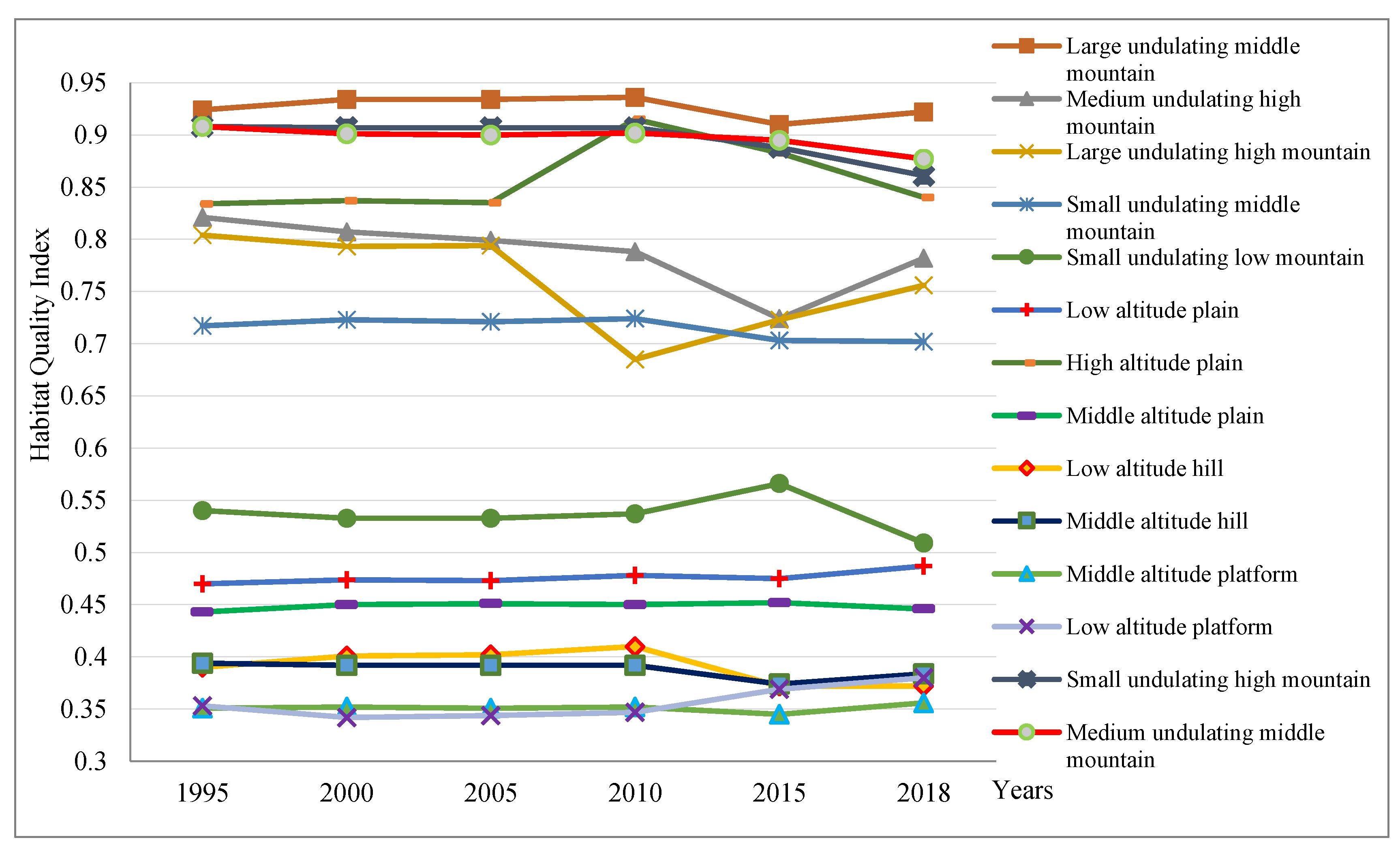
For 14 small-scale geomorphic type units (Figure 7), the order of habitat quality from good to bad was large undulating middle mountain > medium undulating middle mountain > small undulating high mountain > high altitude plain > medium undulating high mountain > large undulating high mountain > small undulating middle mountain > small undulating low mountain > low altitude plain > medium altitude plain > low altitude hills > medium altitude hills > low altitude platform > medium altitude platform.
From Figure 7, we can see from 1995 to 2018, the average habitat quality index of large undulating middle mountain was greater than 0.9, belonging to excellent habitat (0.9–1.0). The average habitat quality index of medium undulating middle mountain, small undulating high mountain, and high altitude plain were all above 0.8, so these three geomorphic types belonged to good habitat (0.8, 0.9). The average habitat quality index of medium undulating high mountain, large undulating high mountain, small undulating middle mountain, and small undulating low mountain were between 0.5–0.8, belonging to general habitat (0.5, 0.8). The average habitat quality index of low altitude plain, medium altitude plain, low altitude hill, medium altitude hill, low altitude platform, and medium altitude platform were all less than 0.5, so these six geomorphic types belonged to poor habitat (0, 0.5).
In Figure 7, from 1995 to 2010, the habitat quality index of large undulating high mountain and high altitude plain fluctuated greatly, while the habitat quality index of other geomorphic types was relatively stable and remained basically unchanged. After 2010, the habitat quality of various geomorphic types began to fluctuate significantly. Among them, high altitude plain, large undulating high mountain, medium undulating high mountain, and small undulating low mountain changed greatly. Although the habitat quality of high altitude plain had remained good (>0.8) in the past 30 years, it increased significantly from 0.835 in 2005 to 0.915 in 2010 and reached excellent habitat (0.9–1.0). Then the habitat quality index began to decline slowly, and finally decreased to 0.84 in 2018. The habitat quality index of large undulating high mountain decreased significantly from 2005 to 2010, from 0.794 to 0.685, and then the habitat quality improved, rising to 0.782 slowly in 2018. The habitat quality index of medium undulating high mountain declined from 0.821 (1995) to 0.724 (2015), and then improved to 0.782 in 2018. The habitat quality of small undulating low mountain remained stable in the first two decades, then reached the maximum in 2015 (0.566), and then decreased to the lowest value of 0.509 (2018). The habitat quality was different in different geomorphic types. The habitat quality in the areas with large fluctuation and high altitude was generally better than that in the areas with medium and low altitude. The geomorphic type with the best habitat quality was the large undulating middle mountain, and the worst was the medium altitude platform.

3.4. Spatial Exploration and Correlation Analysis of Habitat Quality

3.4.1. Spatial Hot Spot Analysis of Habitat Quality

Taking 14 small-scale geomorphic type units as the research object, we used global Morans’I and hotspot analysis to further explore the spatial distribution characteristics and laws of habitat quality under the control of different geomorphic types. The study showed (Figure 8) that from 1995 to 2018, the global Morans’I of habitat quality was all greater than 0, indicating that the habitat quality in the study area showed a certain spatial aggregation. The global Morans’I decreased from 0.407584 in 1995 to 0.363143 in 2015 and increased to 0.384504 in 2018, indicating that there was a trend of spatial aggregation from 1995 to 2018, however, the spatial agglomeration tended to disperse from 1995 to 2015.
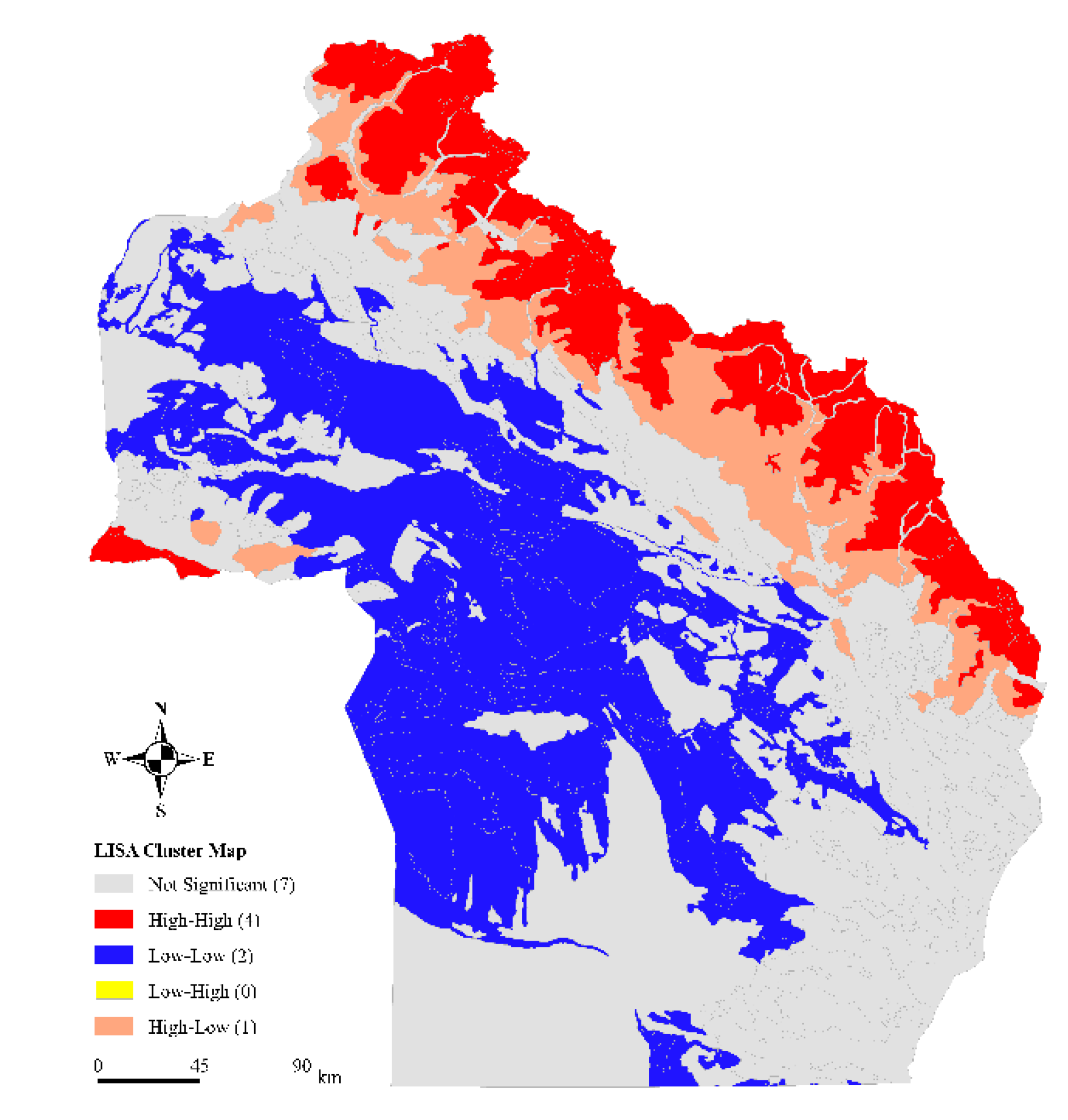
This paper used spatial hotspot analysis to study habitat quality in 2018. The study showed that the habitat quality in the study area had significant cold and hot spots distribution characteristics (Figure 9). The habitat quality of different geomorphic types showed obvious spatial aggregation and showed a banded-step distribution. Altitude from high to low followed by hot spots area, sub hot spots area, insignificant area, and cold spots area. Habitat quality was realized as high–high aggregation, that is, hot spots area, mainly occurring in high mountain and high altitude plain, including four geomorphic types: large undulating high mountain, medium undulating high mountain, small undulating high mountain, and high altitude plain. High–low aggregation, that is, sub hot spots area, mainly occurred in the medium undulating middle mountain. Low–low aggregation, that is, cold spots area, occurred in low altitude areas, including two geomorphic types: low altitude platform and low altitude plain. The spatial aggregation phenomenon was not obvious in the medium altitude area, including 7 geomorphic types: small undulating middle mountain, large undulating middle mountain, small undulating low mountain, medium altitude plain, medium altitude platform, medium altitude hill, and low altitude hill. The difference of cold and hot spots distribution characteristics in the study area was mainly determined by the influence of geographical environmental factors on the scope and intensity of human activities. Human activities in high altitude mountain areas were limited by topography, so human interference to the ecological environment was less. In addition, the vegetation cover density in these areas was large, so the habitat quality remains good, which was hot spots area of habitat quality. The main reason for the difference of cold and hot spots distribution characteristics in the study area was the geomorphic types and human activities. In high mountain areas and high altitude plain areas, forestland was densely distributed and human activities were weak. These places maintain the original state of natural ecology, so they were hot spots areas of habitat quality. In low altitude platform and low altitude plain areas, the main land use types were high coverage grassland, medium coverage grassland, cultivated land and construction land. These two geomorphic types were cold spots areas of habitat quality. In the cold spots area, human activities intensity was high, mainly including over reclamation, overgrazing, mineral development, and construction of industrial and mining, which resulted in grassland degradation, land desertification, salinization, and ecological environment degradation, and finally leading to the reduction of habitat quality.
In medium undulating middle mountain area, shrub wood, sparse wood, and low coverage grassland were mainly distributed, which were mainly secondary hot spots. These areas were mainly affected by grazing. Due to the gradual increase of grazing range and quantity, there was great consumption of river valley forest and shrub forest, resulting in the gradual desertification of desert areas on both sides of the river valley.

3.4.2. Effects of Land Use Change on Habitat Quality

To explore the impact of land use on habitat quality, we made statistics on the habitat quality of different land use types (Figure 10). From 1995 to 2018, the habitat quality index of forestland was the best, followed by water area and grassland, and the lowest habitat quality index was construction land. From 1995 to 2018, the habitat quality index values of forestland and unused land did not change significantly, and the water area showed a trend of first decreasing, then increasing, and then decreasing. From 1995 to 2010, habitat quality index of cultivated land and grassland remained basically unchanged, and the cultivated land showed a downward trend in 2015 and 2018, while the grassland increased first and then decreased. From 1995 to 2005, construction land remained basically unchanged, and there was a sustained increase from 2010 to 2018. The habitat quality index of cultivated land, grassland, water area, and construction land might be disturbed by human activities. With the increase of population, people’s demand for cultivated land and construction land increased, and more grassland was reclaimed as cultivated land. In addition, overgrazing converts grassland into unused land, and natural lakes and canals had been artificially transformed into pit-ponds, which all increased the impact of threat factors. However, it should be noted that although the cultivated land continues to grow, due to the impact of natural disasters, such as drought, sandstorm, and saline-alkali, leading to the simultaneous existence of farmland reclamation and abandonment, this directly had a great impact on suitable wasteland resources and desert grassland. Due to human transformation, the original ecological environment had been destroyed. Land use habitat affected by negative interference had degraded, resulting in the decline of biodiversity and habitat quality. However, after human positive interference, such as returning farmland to forest and grassland and the implementation of relevant ecological protection policies, the habitat degradation degree of land use types disturbed by human factors had decreased and the habitat quality had been improved. From 1995 to 2018, the habitat quality index of forest land had been maintained at a high level above 0.95. This was because the forestland in the Altay region was mostly distributed in high altitude and large fluctuation areas, and the mountainous area was not conducive to reclamation, housing construction, and other activities. Although habitat quality of forestland had maintained a high level, it showed a slow downward trend, which was due to the habitat degradation of forestland caused by logging, deforestation, and reclamation. However, due to the limitation of geomorphic conditions, human activities were restricted. Moreover, the vegetation coverage was high, so its anti-interference ability was strong. Coupled with the implementation of various ecological protection policies and restoration behavior, the habitat quality had always remained at a high level.
To further explore the changes of habitat quality and its main influencing factors under different geomorphic types, the contribution index of land use to habitat quality under various geomorphic types was calculated by using the concept of index contribution, and the correlation between habitat quality and land use types was also discussed (Table 12).
Different geomorphic types contained different land use types (Table 12), so it is necessary to study the relationship between land use types and habitat quality under different geomorphic types. The main contribution indicators and significant correlation factors of different geomorphic types were different. For example, the large undulating high mountain only contains grassland, forestland, and some water bodies, without cultivated land and construction land, while the low altitude areas include almost all land use types. In different geomorphic types, the contribution of land types to habitat quality was also different. In mountainous areas, the indicators with a large contribution to habitat quality were mostly concentrated in grassland and forest land, while in platform, hill, and plain area grassland, Gobi and bare rock gravel land contribute greatly. The significant correlation factors were concentrated in dryland, forestland, grassland, and canals.
For high mountain area, the contribution of forestland and grassland was large, and the significant correlation factors were concentrated in forestland and high coverage grassland. For middle mountain area, the contribution of forestland and grassland was still large, and the significant correlation factors were concentrated in woodland, shrub wood, high coverage grassland, and medium coverage grassland. For low mountainous area, the land use types that contributed greatly to habitat quality were bare rock gravel land (48.68%), low coverage grassland (30.43%), and Gobi (27.39%), and the significant correlation factors included sparse wood, high/medium/low coverage grassland, channel, and rural residential area. For platform area, medium/low coverage grassland, Gobi and bare rock gravel land contributed greatly, but the significant correlation factors between medium altitude platform and low altitude platform were quite different. The former had only beach, while the latter included dryland, low coverage grassland, channel, lake, Gobi, and saline-alkali land. For hill area, the indicators with greater contribution include Gobi and bare rock gravel land, and the bare rock gravel land was a significant correlation factor. However, hills with different undulations had different main contribution indicators. Low coverage grassland (18.22%) had a greater contribution to medium altitude hill, while sand land (88.22%) had a greater contribution to low altitude hill. For plain area, in high altitude, the main contribution indicators were woodland (15.67%), shrub wood (8.31%), high coverage grassland (44.09%), and the significant correlation factors were woodland, shrub wood, medium coverage grassland, permanent glacier, and snowfield. The main contribution indicators of medium/low altitude plain areas were concentrated in grassland and Gobi, and the significant correlation factors were dryland, sparse wood, low coverage grassland, and bare land.
On the whole, indicators that contributed more to the habitat quality of mountain areas in the study area were mostly grassland and forestland, and indicators that contributed more to the platform, hill, and plain areas were mostly grassland, Gobi, and bare rock gravel land. The significant correlation factors were concentrated in dryland, forestland, grassland, and canals. The negative correlation indicators were mainly reflected in the types of unused land, urban land, rural residential area, industrial and mining land, and dryland in cultivated land.

4. Discussion

4.1. Effects of Land Use Change on Habitat Quality from 1995 to 2018

The earth’s surface is the home for human survival. Physiognomy is one of the basic elements in the earth’s surface system, which directly or indirectly affects human life, production, and socio-economic activities. The Altay region has complex and diverse geomorphic types. It is necessary to study habitat quality change based on different geomorphic types, but the relevant research has not been carried out until now. Therefore, based on the extraction of different geomorphic types and land use interpretation maps of six periods from 1995 to 2018, we used the InVEST habitat quality model to estimate habitat quality, to reveal the changing trend of habitat quality under different geomorphic types and the impact of land type on habitat quality.
The results showed that land use had been changing over the past few decades. Unused land, grassland, and forestland were the main land use types in the Altay region. In this period, due to the revitalization of rural areas and the development of rural tourism, the Altay region had tapped the potential of Regional Advantageous tourism resources. It had accelerated the construction of rural public infrastructure and promoted the sustainable development of rural tourism in the Altay area. These measures had provided support for solving poverty in rural areas, but they also had a serious negative impact on the ecological environment and the quality of habitat had decreased [88,89,90]. Economic construction and urban expansion, the areas of cultivated land, urban land, rural residential area, industrial and mining land had proliferated, and the areas of grassland and unused land continued to decrease, which were also important reasons for the decline of ecological environment quality in the study area [48]. People illegally reclaimed land and abandoned land in agricultural expansion promote land desertification [91]. At the same time, blind development from the perspective of land use without effective consideration of the integrity of the ecological environment is likely to cause certain damage to the surrounding ecological environment, and even various irrational development phenomena of the ecological environment. For example, when developing unused land in mountainous and hilly areas, soil erosion may occur due to changes in topography. Grassland overgrazing and degradation, continuous expansion, and occupation of cultivated land and construction land might be the reasons for the reduction of grassland and unused land area.
Land use types and geomorphic types had an important impact on habitat quality. The habitat quality of forest land distributed in large undulating, middle/high altitude area was the best, while that of construction land distributed in small undulating, middle/low altitude area was the worst. The northern part of the Altay region has better habitat quality than the southern, which promoted biodiversity [92] and environmental regulation. The sources of the threats are more severe in the southern part of the Altay region than in its northern part. Due to the natural background, the southern part is mostly desert, bare rock, and gravel land, etc., and the extreme lack of water resources, coupled with unreasonable agricultural expansion, resulted in abandonment and salinization. In addition, overgrazing has contributed to desertification of grasslands, all of which have increased the threat to habitat quality.
The existence of protected areas contributed significantly to alleviating habitat quality in the area [93]. In recent years, with the rapid development of the local economy, overgrazing and mining, inappropriate tourism development, water resources development, and agricultural development, the degradation of the ecosystem of Altai Mountain in the northern part of the study area and the source basins of Irtysh River and Ulungur River in the middle part to a certain extent. Therefore, the “national strategic action plan for biodiversity protection” of the Ministry of environmental protection plans ‘Altai mountain forest grassland ecological function area’ as one of the main protection areas, aiming at regulating habitat quality and protecting biodiversity in the Altai mountain area. Over the past two decades, cultivated land, grassland, water area, and construction land had been positively and negatively disturbed by human activities, resulting in habitat fluctuations. Negative disturbances include continuous expansion of cultivated land and construction land, reclamation of grassland into cultivated land, excessive use of grassland into unused land, and artificial transformation of river channels into pit-ponds. However, due to the positive interference of ecological protection policies such as returning farmland to forest and grassland and the implementation of ecological restoration in the mining area, the degree of habitat degradation had decreased, and the habitat quality has been improved. The habitat quality threats of identification and sensitivity analysis for the Altay region were consistent with the study by Liu et al. [37].
Human activities were an important driving force for changing land use patterns, while physiognomy is an important factor affecting human activities. In low altitude areas, human activities had a wide range and high intensity. The land use types were mainly grassland, cultivated land, urban land, rural residential area, industrial and mining land. To meet material and resource needs, there was a large amount of land reclamation and overgrazing. Reclamation was the main source of cultivated land increase, but affected by some natural disasters, such as drought, sandstorm, and saline-alkali, leading to the simultaneous existence of farmland reclamation and abandonment, which directly had a great impact on the resources suitable for reclamation and desert grassland. The Altay region of Xinjiang is one of the important pastoral areas in China and the residential area of Kazak nationality. Animal husbandry is an important guarantee for economic prosperity and political stability in the region. However, the pasture area in the Altay region is still dominated by extensive livestock farming at the present stage, and there is no regular rotational grazing. For a long time, extensive management and year-round grazing have resulted in overgrazing and overgrazing, resulting in degradation and desertification of natural grassland. In addition, part of the grassland had been reclaimed as cultivated land, resulting in the reduction of grassland and the decline of ecological function. The above contents are the main reasons for the decline of habitat quality. In the middle mountain area, sparse wood, shrub wood, and low coverage grassland are mainly distributed. Due to the gradual increase of grazing range and quantity, there was great consumption of river valley forest and shrub wood, resulting in the gradual desertification of desert areas on both sides of the river valley. In addition, natural factors are also the reasons for the severe ecological environment situation in the study area. The Altay region is located in the middle of the Eurasian continent with high latitude. Its climate is a continental temperate cold climate, and the annual evaporation is greater than the annual precipitation. Due to the small precipitation, there was not enough precipitation during the grass pumping period. In addition, the high temperature was not conducive to the growth and development of grass, which was also one of the factors for the decline of vegetation in grassland animal husbandry area.

4.2. Effects of Geomorphic Types on Habitat Quality and Suggestions for Ecological Management

According to the spatial polarization theory, the development and change of things will make the internal units of the same polarization layer converge and the units of different polarization layers diverge, and each unit in the same polarization layer has two effects on the surrounding units: one is that the blocking effect of dominant units on surrounding units; the second is the promoting effect and the driving effect of surrounding advantageous units on the central unit [94,95,96]. Relevant studies are often based on this theory. According to the effects of spatial diffusion (high–high, low–low) and spatial polarization (high–low, low–high), the results of spatial autocorrelation are zoned, and the zoning protection scheme is put forward [97]. Based on the spatial polarization theory, combined with the habitat quality grade evaluation results and autocorrelation analysis results of the Altay area, this study divides the study area into four types of ecological management schemes: restricted construction area, moderate development area, key restoration area, and comprehensive restoration area. According to the current situation of land development and utilization and its geomorphic types, from the perspective of harmonious and sustainable development between man and nature, this paper puts forward ecological management and protection measures in line with the actual situation.
The four geomorphic types, such as undulating high mountain, are high–high aggregation areas with good habitat quality, and the habitat quality index is greater than 0.5. The land types are mainly forestland and grassland, which are relatively concentrated. However, industrial and mining construction land has appeared in some areas. In order to protect the ecology, these areas can be set as a restricted construction area, strengthening natural ecological protection and prohibiting industrial and mining construction.
The geomorphic type of medium undulating middle mountain is high–low aggregation area, and the habitat quality index is greater than 0.8. The main land types are forest land and grassland but cultivated land and construction land tend to increase. It can be set as moderate development area, focusing on protecting forestland, grassland, and cultivated land with good quality, improving areas with poor quality, and moderately carrying out non-agricultural construction.
The geomorphic types of low altitude platform and low altitude plain are low–low aggregation areas. The habitat quality is poor, and the index is less than 0.5. Six land types are widely distributed, with strong interference from human activities. These areas can be set as key restoration areas, and the current land use situation should be considered comprehensively to appropriately reduce cultivated land and construction land, improve the coverage of forest land and grassland, and finally improve the habitat quality.
The spatial aggregation phenomenon was not obvious in the remaining seven geomorphic types, such as small undulating middle mountain, are set as comprehensive restoration areas for comprehensive restoration. According to the grade of habitat quality and main threat factors of various geomorphic types, targeted restoration work shall be carried out to prevent it from developing in a worse direction.

4.3. Limitations of Uncertainty and Future Recommended Works

In general, compared with previous related studies, the major innovation of this study was to introduce geomorphic types to explore habitat quality under different geomorphic types. The InVEST model used in this paper provides a feasible method for habitat quantification in different geomorphic types and showed the calculation results intuitively. However, due to data limitations, this study only considered the impact of internal threat sources on habitat quality in the study area and did not consider the impact of external threat sources, which may lead to certain errors in the assessment results. At the same time, some parameter indicators were obtained from previous research results and expert experience, the internal mechanisms of the habitat were complex, and different regions had large differences, which will also introduce uncertainty and affect the assessment results. In future research, the threat factors in the marginal portions of the study area will be combined at the same time. We will also further consider the internal mechanisms of habitat quality, and strengthen the local parameterization based on field survey data to more accurately evaluate the spatiotemporal variation characteristics of habitat quality. In addition, this paper only studied the temporal and spatial characteristics of habitat quality under different geomorphic types from the perspective of land use types. In the future, we will combine this with other ecosystem modules to comprehensively consider the ecological effects of land use changes to provide a scientific reference for the sustainable and healthy development of ecosystems in the Altay region.

5. Conclusions

With the economic construction and development in Northwest China, as an important ecological barrier in the core area of economic construction in border areas, the Altay region is affected by various policies and human activities, such as urban and tourism development [98], thus seriously affecting the structure and function of ecosystems and the sustainable use of ecotourism resources. The results also showed that there had been a significant land use change in the study area over the past three decades. In this period, due to the economic construction and urban expansion, the areas of cultivated land and construction land had proliferated, and the areas of grassland and unused land continued to decrease, causing a serious negative impact on the ecological environment and declining the habitat quality in the Altay region. Therefore, we recommend ecological restoration measures to realize the coordinated development of regional economy, society, and ecology. It is worth noting that vegetation cover has decreased rapidly, agricultural activities have increased, and urban land, rural residential land, and industrial and mining land have increased. Unreasonable use of water resources led to land salinization in desert areas. Desertification was caused by blind reclamation of oases. The increase of human disturbance had seriously degraded the local ecosystem, promoted the destruction of the natural environment, and increased the disturbance to habitat, which seriously threatens human well-being.
The findings indicated that in different geomorphic types of land use types, habitat quality and the contribution of land use types to habitat quality were all different and showed great differences. Therefore, to improve the regional habitat quality, the land management strategy of “adjusting measures to local conditions” should be adopted according to different geographical environment backgrounds and the degree of habitat quality decline. This requires necessary ecological restoration and biodiversity protection and control actions in this location.

Author Contributions

Conceptualization, B.W. and W.C.; methodology, B.W. and W.C.; software, B.W.; validation, B.W.; formal analysis, B.W.; investigation, B.W.; resources, B.W. and W.C.; data curation, B.W. and W.C.; writing—original draft preparation, B.W.; writing—review and editing, B.W.; visualization, B.W.; funding acquisition, W.C. All authors have read and agreed to the published version of the manuscript.

Funding

This research was funded by the National Natural Science Foundation of China (42130110), the Bureau of Science and Technology of Altay region, Ili Kazak Autonomous Prefecture (Y99M4600AL), and Xinjiang Scientific Investigation Basic Geographic Information Database (2021xjkk1301).

Institutional Review Board Statement

Not applicable.

Informed Consent Statement

Not applicable.

Data Availability Statement

Data sharing not applicable.

Acknowledgments

The authors would like to thank for the data support form “Resource and Environment Science and Data Center (https://www.resdc.cn/Default.aspx, accessed on 13 July 2021) for providing 1 km LUCC data for reference, and China Centre For Resources Satelite Data and Application (http://36.112.130.153:7777/DSSPlatform/productSearch.html, accessed on 21 March 2019) for providing remote sensing image data”. We also wished to thank Yongping Liu, Liyan Liu, and Yurong Hou for their assistance in land use sampling.

Conflicts of Interest

The authors declare no conflict of interest.

References

  1. Dai, L.; Li, S.; Lewis, B.J.; Wu, J.; Yu, D.; Zhou, W.; Zhou, L.; Wu, S. The influence of land use change on the spatial–temporal variability of habitat quality between 1990 and 2010 in Northeast China. J. For. Res. 2019, 30, 2227–2236. [Google Scholar] [CrossRef]
  2. Rands, M.R.W.; Adams, W.M.; Bennun, L.; Butchart, S.H.M.; Clements, A.; Coomes, D.; Entwistle, A.; Hodge, I.; Kapos, V.; Scharlemann, J.P.W.; et al. Biodiversity conservation: Challenges beyond 2010. Science 2010, 329, 1298–1303. [Google Scholar] [CrossRef] [PubMed] [Green Version]
  3. Terrado, M.; Sabater, S.; Chaplin-Kramer, B.; Mandle, L.; Ziv, G.; Acuna, V. Model development for the assessment of terrestrial and aquatic habitat quality in conservation planning. Sci. Total Environ. 2016, 540, 63–70. [Google Scholar] [CrossRef] [PubMed] [Green Version]
  4. Gaglio, M.; Lanzoni, M.; Nobili, G.; Viviani, D.; Castaldelli, G.; Fano, E.A. Ecosystem services approach for sustainable governance in a brackish water lagoon used for aquaculture. J. Environ. Plan. Manag. 2019, 62, 1501–1524. [Google Scholar] [CrossRef]
  5. Wu, Y.; Tao, Y.; Yang, G.; Ou, W.; Pueppke, S.; Sun, X.; Chen, G.; Tao, Q. Impact of land use change on multiple ecosystem services in the rapidly urbanizing Kunshan City of China: Past trajectories and future projections. Land Use Policy 2019, 85, 419–427. [Google Scholar] [CrossRef]
  6. Mashizi, A.K.; Escobedo, F.J. Socio-ecological assessment of threats to semi-arid rangeland habitat in Iran using spatial models and actor group opinions. J. Arid. Environ. 2020, 177, 104136. [Google Scholar] [CrossRef]
  7. Ellis, E.C.; Pascual, U.; Mertz, O. Ecosystem services and nature’s contribution to people: Negotiating diverse values and trade-offs in land systems. Curr. Opin. Environ. Sustain. 2019, 38, 86–94. [Google Scholar] [CrossRef]
  8. Musacchio, L.R. Cultivating deep care: Integrating landscape ecological research into the cultural dimension of ecosystem services. Landsc. Ecol. 2013, 28, 1025–1038. [Google Scholar] [CrossRef]
  9. Hillard, E.M.; Nielsen, C.K.; Groninger, J.W. Swamp rabbits as indicators of wildlife habitat quality in bottomland hardwood forest ecosystems. Ecol. Indic. 2017, 79, 47–53. [Google Scholar] [CrossRef]
  10. Riedler, B.; Lang, S. A spatially explicit patch model of habitat quality, integrating spatio-structural indicators. Ecol. Indic. 2017, 94, 128–141. [Google Scholar] [CrossRef]
  11. Zhao, G.S.; Liu, J.Y.; Kuang, W.H.; OuYang, Z.Y.; Xie, Z.L. Disturbance impacts of land use change on biodiversity conservation priority areas across China: 1990-2010. J. Geogr. Sci. 2015, 25, 515–529. [Google Scholar] [CrossRef] [Green Version]
  12. Gao, Y.; Ma, L.; Liu, J.; Zhuang, Z.; Huang, Q.; Li, M. Constructing Ecological Networks Based on Habitat Quality Assessment: A Case Study of Changzhou, China. Sci. Rep. 2017, 7, 46073. [Google Scholar] [CrossRef] [PubMed]
  13. Postek, P.; Leń, P.; Stręk, Ż. The proposed indicator of fragmentation of agricultural land. Ecol. Indic. 2019, 103, 581–588. [Google Scholar] [CrossRef]
  14. Niquisse, S.; Cabral, P. Assessment of changes in ecosystem service monetary values in Mozambique. Environ. Dev. 2018, 25, 12–22. [Google Scholar] [CrossRef]
  15. Wang, L.; Lyons, J.; Kanehl, P.; Gatti, R. Influences of Watershed Land Use on Habitat Quality and Biotic Integrity in Wisconsin Streams. Fisheries 1997, 22, 6–12. [Google Scholar] [CrossRef]
  16. Ren, H.; Zhang, J.J.; Zhu, W.B.; Wang, L.Y.; Zhang, L.J.; Zhu, L.Q. Impact of land use change on habitat in the Qihe River Basin ofTaihang Mountains. Prog. Geogr. 2018, 37, 1693–1704. [Google Scholar] [CrossRef]
  17. Mckinney, M.L. Urbanization, Biodiversity, and Conservation. Bioscience 2002, 52, 883–890. [Google Scholar] [CrossRef]
  18. Fu, B.J.; Zhang, L.W. Land-Use Change and Ecosystem Services: Concepts, Methods and Progress. Prog. Geogr. 2014, 33, 441–446. [Google Scholar] [CrossRef]
  19. Liu, M.X. Biodiversity Characters and Eco-Environment Quality Evaluation on Nature Reserve of Xihu in Dunhuang. J. Arid. Land Resour. Environ. 2009, 23, 171–175. [Google Scholar] [CrossRef]
  20. Liu, H.; Cai, Y.; Yu, M.Q.; Gong, H.T.; An, S.Q. Assessment of River Habitat Quality in Yixing District of Taihu Lake Basin. Chin. J. Ecol. 2012, 31, 1288–1295. [Google Scholar] [CrossRef]
  21. Yang, J.Q.; Zhu, Y.G.; Song, W.P.; Zhang, J.; Zhang, L.J.; Luo, X.X. The Eco-Environmental Evaluation Based on Habitat Quality and Ecological Response of Laizhou Bay. Acta Ecol. Sin. 2014, 34, 105–114. [Google Scholar] [CrossRef]
  22. Sharp, R.; Tallis, H.T.; Ricketts, T.; Guerry, A.D.; Wood, S.A.; Chaplin-Kramer, R.; Nelson, E.; Ennaanay, D.; Wolny, S.; Olwero, N.; et al. InVEST 3.6.0 User’s Guide; Collaborative Publication by The Natural Capital Project, Stanford University, the University of Minnesota, The Nature Conservancy, and the World Wildlife Fund; Stanford University: Stanford, CA, USA, 2018; Available online: https://naturalcapitalproject.stanford.edu/software/invest (accessed on 3 April 2021).
  23. Tallis, H.; Ricketts, T.; Guerry, A. InVEST User’s Guide: Integrated Valuation of Environmental Services and Tradeoffs; Collaborative Publication by The Natural Capital Project, Stanford University, the University of Minnesota, The Nature Conservancy, and the World Wildlife Fund; Stanford University: Stanford, CA, USA, 2013. [Google Scholar]
  24. Sherrouse, B.C.; Semmens, D.J.; Clement, J.M. An application of Social Values for Ecosystem Services (SolVES) to three national forests in Colorado and Wyoming. Ecol. Indic. 2014, 36, 68–79. [Google Scholar] [CrossRef]
  25. Hengl, T.; Sierdsema, H.; Radović, A.; Dilo, A. Spatial prediction of species’ distributions from occurrence-only records: Combining point pattern analysis, ENFA and regression-kriging. Ecol. Model. 2009, 220, 3499–3511. [Google Scholar] [CrossRef] [Green Version]
  26. Urban, M.C.; Bocedi, G.; Hendry, A.P.; Mihoub, J.B.; Pe’Er, G.; Singer, A.; Bridle, J.R.; Crozier, L.G.; Meester, L.D.; Godsoe, W. Improving the forecast for biodiversity under climate change. Science 2016, 353, aad8466. [Google Scholar] [CrossRef] [PubMed] [Green Version]
  27. Reyers, B. Natural Capital: Theory and Practice of Mapping Ecosystem Services. J. Integr. Environ. Sci. 2013, 10, 141–143. [Google Scholar] [CrossRef] [Green Version]
  28. Polasky, S.; Nelson, E.; Pennington, D.; Johnson, K.A. The Impact of Land-Use Change on Ecosystem Services, Biodiversity and Returns to Landowners: A Case Study in the State of Minnesota. Env. Resour. Econ. 2013, 48, 219–242. [Google Scholar] [CrossRef]
  29. Li, J.; Gong, J.; Guldmann, J.-M.; Li, S.; Zhu, J. Carbon Dynamics in the Northeastern Qinghai–Tibetan Plateau from 1990 to 2030 Using Landsat Land Use/Cover Change Data. Remote Sens. 2020, 12, 528. [Google Scholar] [CrossRef] [Green Version]
  30. Sallustio, L.; Toni, A.D.; Strollo, A.; Febbraro, M.; Gissi, E.; Casella, L.; Geneletti, D.; Munafò, M.; Vizzarri, M.; Marchetti, M. Assessing habitat quality in relation to the spatial distribution of protected areas in Italy. J. Environ. Manag. 2017, 201, 129–137. [Google Scholar] [CrossRef]
  31. Berta Aneseyee, A.; Noszczyk, T.; Soromessa, T.; Elias, E. The InVEST Habitat Quality Model Associated with Land Use/Cover Changes: A Qualitative Case Study of the Winike Watershed in the Omo-Gibe Basin, Southwest Ethiopia. Remote Sens. 2020, 12, 1103. [Google Scholar] [CrossRef] [Green Version]
  32. Gong, J.; Ma, X.C.; Zhang, L.L.; Liu, D.Q.; Zhang, J.X. Spatialtemporal Variation of Habitat Quality in Bailongjiang Watershed in Gansu Based on InVEST Model. Res. Soil Water Conserv. 2018, 25, 191–196. [Google Scholar] [CrossRef]
  33. Mushet, D.M.; Neau, J.L.; Euliss, N.H. Modeling effects of conservation grassland losses on amphibian habitat. Biol. Conserv. 2014, 174, 93–100. [Google Scholar] [CrossRef]
  34. Mekonnen, T.; Aticho, A. The Driving Forces of Boye Wetland Degradation and Its Bird Species Composition, Jimma, Southwestern Ethiopia. Int. J. Ecol. Dev. 2012, 3, 365–369. [Google Scholar] [CrossRef]
  35. Du, S.X.; Rong, Y.J. The Biodiversity Assessment of Land Use in ShanXi Province Based on InVEST Model. Environ. Sustain. Dev. 2015, 40, 65–70. [Google Scholar] [CrossRef]
  36. Chen, Y.; Qiao, F.; Jiang, L. Effects of Land Use Pattern Change on Regional Scale Habitat Quality Based on InVEST Model—A Case Study in Beijing. Acta Sci. Nat. Univ. Pekin. 2016, 52, 553–562. [Google Scholar] [CrossRef]
  37. Liu, F.T.; Xu, E.Q. Comparison of Spatial-Temporal Evolution of Habitat Quality between Xinjang Corps and Noncorps Region Based on Land Use. Chin. J. Appl. Ecol. 2020, 31, 2341–2351. [Google Scholar] [CrossRef]
  38. Zhao, S.Q.; Dai, X.; Shen, Y.C.; Yang, L.L. Land Types and Their Distribution in the Heilongjiang Province and Hulunbeier League. Geogr. Res. 1982, 1, 49–57. Available online: https://kns.cnki.net/kcms/detail/detail.aspx?FileName=DLYJ198201007&DbName=CJFQ1982 (accessed on 19 December 2021).
  39. Cheng, W.M.; Zhou, C.H. Methodology on Hierarchical Classification of Multi-Scale Digital Geomorphology. Prog. Geogr. 2014, 33, 23–33. [Google Scholar] [CrossRef]
  40. Iwahashi, J.; Pike, R.J. Automated classifications of topography from DEMs by an unsupervised nested-means algorithm and a three-part geometric signature. Geomorphology 2007, 86, 409–440. [Google Scholar] [CrossRef]
  41. Drăguţ, L.; Eisank, C. Automated object-based classification of topography from SRTM data. Geomorphology 2012, 141–142, 21–33. [Google Scholar] [CrossRef] [Green Version]
  42. Summerfield, M.A. Geomorphology and Global Tectonics; John Wiley & Sons Ltd.: UK, Chichester, 2000. [Google Scholar]
  43. Mka, B.; Pmbac, D.; Sr, E.; Db, E.; Ad, B. A planning-support tool for spatial suitability assessment of green urban stormwater infrastructure. Sci. Total Environ. 2019, 686, 856–868. [Google Scholar] [CrossRef]
  44. Samer, M. Towards the implementation of the Green Building Concept in Agricultural Buildings: A Literature Review. Agric. Eng. Int. CIGR E-J. 2013, 15, 25–46. Available online: https://www.researchgate.net/publication/245543328 (accessed on 19 December 2021).
  45. Wang, S.J.; Cheng, W.M.; Shi, Q.S. Analysis on Internal Mechanisms of the Life Community of Mountain, River, Forest, Field, Lake and Grass at Watershed Scale. J. Xinjiang Univ. Nat. Sci. Ed. Chin. Engl. 2021, 38, 313–320. [Google Scholar] [CrossRef]
  46. Mai, H.C. Discussion on the Distribution and Development of Mineral Resources in Altay, Xinjiang. Miner. Resour. 2021, 107–108. Available online: https://kns.cnki.net/kcms/detail/detail.aspx?FileName=COLO202105054&DbName=CJFQ2021 (accessed on 17 December 2021).
  47. Sun, T.S.; Bao, Y.Q.; Li, W.Y. Strategy on the Development of Grass-Based Livestock Husbandry in the Arid and Semi-Arid Region Based on Sustainable Utilization of Grassland Resources: A Case Study of Altay, Xinjiang, China. Chin. J. Ecol. 2020, 39, 3509–3520. [Google Scholar] [CrossRef]
  48. Zhang, W.H.; Lei, L. Present Situation and Cause Analysis of Ecological Environment in Altay Region. Shengtaihuanjing 2017, 29, 262–263. [Google Scholar] [CrossRef]
  49. Ellis, E.A.; Porter-Bolland, L. Is community-based forest management more effective than protected areas?: A comparison of land use/land cover change in two neighboring study areas of the Central Yucatan Peninsula, Mexico. For. Ecol. Manag. 2008, 256, 1971–1983. [Google Scholar] [CrossRef]
  50. Liu, J.Y.; Kuang, W.H.; Zhang, Z.X.; Xu, X.L.; Qin, Y.W.; Ning, J.; Zhou, W.C.; Zhang, S.W.; Li, R.D.; Yan, C.Z.; et al. Spatiotemporal Characteristics, Patterns, and Causes of Land-Use Changes in China since the Late 1980s. J. Geogr. Sci. 2014, 24, 195–210. [Google Scholar] [CrossRef]
  51. Liu, J.Y.; Ning, J.; Kuang, W.H.; Xu, X.L.; Zhang, S.W.; Yan, C.Z.; Li, R.D.; Wu, S.X.; Hu, Y.F.; Du, G.M.; et al. Spatio-Temporal Patterns and Characteristics of Land-Use Change in China during 2010–2015. Acta Geogr. Sin. 2018, 73, 789–802. [Google Scholar] [CrossRef]
  52. Yang, Z.X.; Jia, D.Z.; Zhou, H.Y.; Hu, Y.N.; Li, G. Land-Use Information Extraction of GF-1 Remote Sens. Image of Reservoir Area by Using Object-Oriented Method. Bull. Surv. Mapp. 2020, 35–39. [Google Scholar] [CrossRef]
  53. Zhang, J.; Li, X.D.; Cheng, C.Y.; Liu, J.Y. Analysis of the relief amplitude in Xinjiang. J. Landzhou Univ. Nat. Sci. 2008, 44, 10–13. [Google Scholar] [CrossRef]
  54. Wang, L.; Lv, X. Analysis of the Relief Amplitude in Xinjiang Based on Digital Elevation Model. Sci. Surv. Mapp. 2009, 34, 113–116. [Google Scholar] [CrossRef]
  55. Zhou, C.H.; Cheng, W.M.; Qian, J.K.; Li, B.Y.; Zhang, B.P. Research on the Classification System of Digital Land Geomorphology of 1:1 000 000 in China. J. Geo-Inf. Sci. 2009, 11, 707–724. Available online: https://kns.cnki.net/kcms/detail/detail.aspx?FileName=DQXX200906007&DbName=CJFQ2009 (accessed on 19 December 2021). [CrossRef]
  56. Miliaresis, G.C. Extraction of bajadas from digital elevation models and satellite imagery. Comput. Geosci. 2001, 27, 1157–1167. [Google Scholar] [CrossRef]
  57. Bocco, G.; Mendoza, M.; Velázquez, A. Remote Sens. and GIS-based regional geomorphological mapping- A tool for land use planning in developing countries. Geomorphology 2001, 39, 211–219. [Google Scholar] [CrossRef]
  58. Niekerk, A.V. A comparison of land unit delineation techniques for land evaluation in the Western Cape, South Africa. Land Use Policy 2010, 27, 937–945. [Google Scholar] [CrossRef] [Green Version]
  59. Drăgut, L.; Eisank, C. Object representations at multiple scales from digital elevation models. Geomorphology 2011, 129, 183–189. [Google Scholar] [CrossRef] [Green Version]
  60. Cheng, W.M.; Zhou, C.H.; Li, B.Y.; Shen, Y.C. Geomorphological regionalization theory system and division methodology of China. Acta Geogr. Sin. 2019, 74, 839–856. [Google Scholar] [CrossRef]
  61. Burrough, P.A.; Wilson, J.P.; Gaans, P.F.M.; Hansen, A.J. Fuzzy k-means classification of topo-climatic data as an aid to forest mapping in the Greater Yellowstone Area, USA. Landsc. Ecol. 2001, 16, 523–546. [Google Scholar] [CrossRef]
  62. Mu, Z.G. Study on Identifying Active Faults of Highway Engineering Based on DEM and Knowledge. Master’s Thesis, Changan University, Xi’An, China, 2008. [Google Scholar]
  63. Tu, H.M.; Liu, Z.D. Demonstration on Optimum Statistic Unit of Relief Amplitude in China. J. Hubei Univ. Nat. Sci. 1990, 12, 266–271. Available online: https://kns.cnki.net/kcms/detail/detail.aspx?FileName=HDZK199003016&DbName=CJFQ1990 (accessed on 19 December 2021).
  64. Ding, X.F. Research on the Basic Morphological Types of Land Geomorphology in Funing County, Yunnan Province Based on the SRTM_ DEM and the Change Point Method. Geomat. Spat. Inf. Technol. 2014, 37, 3. [Google Scholar] [CrossRef]
  65. Zhu, J.; Ding, N.; Li, D.; Sun, W.; Xie, Y.; Wang, X. Spatiotemporal Analysis of the Nonlinear Negative Relationship between Urbanization and Habitat Quality in Metropolitan Areas. Sustainability 2020, 12, 669. [Google Scholar] [CrossRef] [Green Version]
  66. Vigiak, O.; Borselli, L.; Newham, L.T.; McInnes, J.; Roberts, A.M. Comparison of Conceptual Landscape Metrics to Define Hillslope-Scale Sediment Delivery Ratio. Geomorphology 2012, 138, 74–88. [Google Scholar] [CrossRef]
  67. Cheng, F.Y.; Liu, S.L.; Hou, X.Y.; Wu, X.; Dong, S.K.; COXIXO, A. The effects of urbanization on ecosystem services for biodiversity conservation in southernmost Yunnan Province, Southwest China. J. Geogr. Sci. 2019, 29, 1159–1178. [Google Scholar] [CrossRef] [Green Version]
  68. OuYang, Z.Y.; Zheng, H. Ecological Mechanisms of Ecosystem Services. Acta Ecol. Sin. 2009, 29, 6183–6188. [Google Scholar] [CrossRef]
  69. Zhang, T.; Gao, Y.; Li, C.; Xie, Z.; Chang, Y.; Zhang, B. How Human Activity Has Changed the Regional Habitat Quality in an Eco-Economic Zone: Evidence from Poyang Lake Eco-Economic Zone, China. Int. J. Environ. Res. Public Health 2020, 17, 6253. [Google Scholar] [CrossRef] [PubMed]
  70. Zhang, X.; Zhou, J.; Li, G.; Chen, C.; Li, M.; Luo, J. Spatial pattern reconstruction of regional habitat quality based on the simulation of land use changes from 1975 to 2010. J. Geogr. Sci. 2020, 30, 601–620. [Google Scholar] [CrossRef]
  71. Otto, C.R.V.; Roth, C.L.; Carlson, B.L.; Smart, M.D. Land-use change reduces habitat suitability for supporting managed honey bee colonies in the Northern Great Plains. Proc. Natl. Acad. Sci. USA 2016, 113, 10430–10435. [Google Scholar] [CrossRef] [Green Version]
  72. Xie, Y.C.; Gong, J.; Zhang, S.X.; Ma, X.C.; Hu, B.Q. Spatiotemporal Change of Landscape Biodiversity Based on InVEST Model and Remote Sens. Technology in the Bailong River Watershed. Sci. Geogr. Sin. 2018, 38, 979–986. [Google Scholar] [CrossRef]
  73. Wu, J.S.; Cao, Q.W.; Shi, S.Q.; Huang, X.L.; Lu, Z.Q. Spatio-temporal variability of habitat quality in Beijing-Tianjin-Hebei Area based on land use change. Chin. J. Appl. Ecol. 2015, 26, 3457–3466. [Google Scholar] [CrossRef]
  74. Tashakkori, A.; Teddlie, C. Issues and dilemmas in teaching research methods courses in social and behavioural sciences: US perspective. Int. J. Soc. Res. Methodol. 2003, 6, 61–77. [Google Scholar] [CrossRef]
  75. Diehl, M.; Wahl, H.W.; Freund, A. Ecological Validity as a Key Feature of External Validity in Research on Human Development. Res. Hum. Dev. 2017, 14, 177–181. [Google Scholar] [CrossRef]
  76. Saaty, T.L.; Vargas, L.G. Prediction, Projection, and Forecasting: Applications of the Analytic Hierarchy Process in Economics, Finance, Politics, Games, and Sports. Kluwer Academic Pub. 1991. Available online: http://www.wkap.com (accessed on 7 June 2019).
  77. Kulimushi, L.C.; Choudhari, P.; Mubalama, L.K.; Banswe, G.T. GIS and Remote Sens.-based assessment of soil erosion risk using RUSLE model in South-Kivu province, eastern, Democratic Republic of Congo. Geomat. Nat. Hazards Risk 2021, 12, 961–987. [Google Scholar] [CrossRef]
  78. Zhong, L.N.; Wang, J. Evaluation on Effect of Land Consolidation on Habitat Quality Based on InVEST Model. Trans. Chin. Soc. Agric. Eng. 2017, 33, 250–255. [Google Scholar] [CrossRef]
  79. Lahiji, R.N.; Dinan, N.M.; Liaghati, H.; Ghaffarzadeh, H.; Vafaeinejad, A. Scenario-based estimation of catchment carbon storage: Linking multi-objective land allocation with InVEST model in a mixed agriculture-forest landscape. Front. Earth Sci. 2020, 14, 10. [Google Scholar] [CrossRef]
  80. Zhang, S.L.; Zhang, K. Contrast Study on Moran and Getis-Ord Indexes of Local Spatial Autocorrelation Indices. J. Geod. Geodyn. 2007, 27, 31–34. [Google Scholar] [CrossRef]
  81. Getis, A.; Ord, J.K. The Analysis of Spatial Association by Use of Distance Statistics. Geogr. Anal. 1992, 24, 189–206. [Google Scholar] [CrossRef]
  82. Anselin, L. Local indicators of spatial association. Geogr. Anal. 1995, 27, 93–115. [Google Scholar] [CrossRef]
  83. Abdulhafedh, A. A Novel Hybrid Method for Measuring the Spatial Autocorrelation of Vehicular Crashes: Combining Moran’s Index and Getis-Ord G* Statistic. Open J. Civ. Eng. 2017, 7, 208–221. [Google Scholar] [CrossRef] [Green Version]
  84. Moran, A.P. Notes on Continuous Stochastic Phenomena. Biometrika 1950, 37, 17–23. [Google Scholar] [CrossRef]
  85. Liang, H.Y.; Zhou, Q.L.; Sun, Y.L. Influence Analysis of Spatial Weight Matrix on Spatial Autocorrelation. Sci. Technol. Inf. 2013, 141–143. [Google Scholar] [CrossRef]
  86. Xu, X. A note on the subjective and objective integrated approach to determine attribute weights. Eur. J. Oper. Res. 2004, 156, 530–532. [Google Scholar] [CrossRef]
  87. Chen, Y.F.; Wang, Y.H.; Zhao, W.J.; Hu, Z.W.; Duan, F.Z. Contributing Factors and Classification of Poor Villages in China. Acta Geogr. Sin. 2017, 72, 1827–1844. [Google Scholar] [CrossRef]
  88. Hu, L.L.; Li, C.L. Coupling and Coordination of Rural Rejuvenation and Rural Tourism in Altay Region of Xinjiang. J. Yunnan Agric. Univ. Soc. Sci. 2021, 15, 8–13. [Google Scholar] [CrossRef]
  89. Laurance, W.F.; Williamson, G.B. Positive feedbacks among forest fragmentation, drought, and climate change in the Amazon. Conserv. Biol. 2001, 15, 1529–1535. [Google Scholar] [CrossRef] [Green Version]
  90. Laurance, W.F.; Balmford, A. Land use: A global map for road building. Nature 2013, 495, 308–309. [Google Scholar] [CrossRef] [PubMed]
  91. Shao, M.L. Analysis on the Problems, Causes and Countermeasures of Rural Ecological Environment Protection in Altay Region. Labor. Prot. World 2015, 51–53. Available online: https://kns.cnki.net/kcms/detail/detail.aspx?FileName=LDBJ201524038&DbName=CJFQ2015 (accessed on 19 December 2021).
  92. Li, N.; Ding, C.C.; Cao, D.D.; Chu, H.J.; Qi, Y.J.; Li, C.W.; Ping, X.G.; Sun, Y.H.; Jiang, Z.G. Avian Species Census, Richness Patterns and Faunal Composition in the Altay Region, China. Biodivers. Sci. 2020, 28, 401–411. [Google Scholar] [CrossRef]
  93. Zhang, Z.; Hao, H.G.; Zhang, Q.; Hu, Z.G. Countermeasures and Suggestions for Continuously Promoting Protection and Restoration of “Mountains, Rivers, Forests, Farmlands, Lakes, Grasslands and Desserts” in Altay Prefecture of Xinjiang. Environ. Sustain. Dev. 2021, 46, 93–98. [Google Scholar] [CrossRef]
  94. Lv, L.C. Plarization, New Polarization and Zhujiang River Delta’s Development. Sci. Geogr. Sin. 2000, 20, 355–361. [Google Scholar] [CrossRef]
  95. Esteban, J.M.; Ray, D. On the Measurement of Polarization. Boston University-Institute for Economic Development: Boston, MA, USA, 1991. [Google Scholar]
  96. Myrdal, G. Economic theory and under-developed regions. In Proceedings of the Aps April Meeting, London, UK, 7–10 April 2019. [Google Scholar]
  97. Chen, L.L.; Song, Y.; Zou, C.H.; Zhou, H.; Zhang, X. Zoning of Protected Cultivated Land Based on Improved Local Indicators of Spatial Association. Resour. Sci. 2016, 38, 1871–1882. [Google Scholar] [CrossRef]
  98. Ding, F.Y. A Research on Development of Homestay Tourism in Aletai Region under the Background of All-for-One Tourism. J. Chang. Univ. 2019, 29, 43–47. Available online: https://kns.cnki.net/kcms/detail/detail.aspx?FileName=CDXB201907008&DbName=CJFQ2019 (accessed on 19 December 2021).
Figure 1. Location and topography of the study area.
Remotesensing 14 01279 g001
Figure 2. Fitting curve of the relationship between grid units and relief amplitude.
Remotesensing 14 01279 g002
Figure 3. S and S i differential value change curve.
Remotesensing 14 01279 g003
Figure 4. The geomorphic maps of the study area ((a) is the distribution of 6 medium-scale geomorphic types; (b) is the distribution of 14 small-scale geomorphic types).
Remotesensing 14 01279 g004
Figure 5. Distribution and changes of land use types in the Altay region from 1995 to 2018.
Remotesensing 14 01279 g005
Figure 6. Spatial distribution of habitat quality in the Altay region from 1995 to 2018.
Remotesensing 14 01279 g006aRemotesensing 14 01279 g006b
Figure 7. Habitat quality change chart of different geomorphic types from 1995 to 2018.
Remotesensing 14 01279 g007
Figure 8. Moran’s I index distribution map of habitat quality from 1995–2018 (1. small undulating high mountain; 2. high altitude plain; 3. medium undulating high mountain; 4. large undulating high mountain; 5. large undulating middle mountain; 6. medium undulating middle mountain; 7. small undulating middle mountain; 8. low altitude platform; 9. low altitude plain; 10. small undulating low mountain; 11. medium altitude plain; 12. medium altitude hill; 13. medium altitude platform; 14. low altitude hill).
Remotesensing 14 01279 g008
Figure 9. Hot spots distribution map of habitat quality in the study area in 2018.
Remotesensing 14 01279 g009
Figure 10. Average habitat quality index of different land use types.
Remotesensing 14 01279 g010
Table 1. Land use classification system.
First ClassSecond Class
1 Cultivated land1-1 Paddy land1-2 Dryland
Remotesensing 14 01279 i001 Remotesensing 14 01279 i002
2 Forestland2-1 Woodland2-2 Shrub wood2-3 Sparse wood2-4 Other woodland
Remotesensing 14 01279 i003 Remotesensing 14 01279 i004 Remotesensing 14 01279 i005 Remotesensing 14 01279 i006
3 Grassland3-1 High coverage grassland3-2 Medium coverage grassland3-3 Low coverage grassland
Remotesensing 14 01279 i007 Remotesensing 14 01279 i008 Remotesensing 14 01279 i009
4 Water area4-1 Canal4-2 Lake4-3 Pit-pond4-4 Shoaly land4-5 Permanent glacier and snowfield
Remotesensing 14 01279 i010 Remotesensing 14 01279 i011 Remotesensing 14 01279 i012 Remotesensing 14 01279 i013 Remotesensing 14 01279 i014
5 Construction land5-1 Urban land5-2 Rural residential area5-3 Industrial and mining land
Remotesensing 14 01279 i015 Remotesensing 14 01279 i016 Remotesensing 14 01279 i017
6 Unused land6-1 Sand land6-2 Gobi6-3 Saline-alkali land6-4 Marsh land6-5 Bare land6-6 Bare rock gravel land
Remotesensing 14 01279 i018 Remotesensing 14 01279 i019 Remotesensing 14 01279 i020 Remotesensing 14 01279 i021 Remotesensing 14 01279 i022 Remotesensing 14 01279 i023
Table 2. The classification system of geomorphological type.
AltitudeLow Altitude (<1000 m)Medium Altitude (1000 m–2400 m)High Altitude (>2400 m)
Relief Amplitude
Plain (Generally < 30 m)Low altitude plainMedium altitude plainHigh altitude plain
Platform (Generally > 30 m)Low altitude platformMedium altitude platformHigh altitude platform
Hill (<200 m)Low altitude hillsMedium altitude hillsHigh altitude hills
Small undulating mountain (200 m–500 m)Small undulating low mountainsSmall undulating middle mountainSmall undulating high mountain
Medium undulating mountain (500 m–1000 m)Medium undulating low mountainMedium undulating middle mountainMedium undulating high mountain
Large undulating mountain (1000 m–1400 m)---Large undulating middle mountainLarge undulating high mountain
Table 3. The meaning of several topographic factors and their mathematical expression.
Topographic FactorsEquationsMeaning
Slope R = Δ H L × 100 The degree of inclination within the surface unit and its neighbourhood.
Surface relief T F = H m a x H m i n It is an important index used to quantitatively describe geomorphic form and divide geomorphic form types. It can reflect the development stage of landform. Most of the “new” geomorphic units have large fluctuation, while the “old” geomorphic units have small surface fluctuation.
Coefficient of variation of elevation V = S / Z
S = [ 1 n 1 k 1 n ( Z k Z ) 2 ] 1 2
Analyse the elevation change within a neighbourhood of the ground point. Most studies use the ratio of the standard deviation of altitude to the mean value in this range.
Table 4. Data input for the habitat quality model.
Input DataDescription
Land use/land coverA standard GIS raster dataset, each cell has a digital LULC code. The LULC raster should include the area of interest and the width buffer for the maximum threat distance. The raster should not contain any other data. The LULC codes must match the sensitivity coding of the land use type to each threat.
Threat dataA CSV table of all threats needed to be considered in the model. The table contains information on each threat’s relative importance or weight and its impact across space. Each row is a threat source. Each column contains a different attribute of each threat source, and must be named as THREAT, MAX-DIST, WEIGHT, and DECAY.
Threat rasterGIS raster files with the distribution and intensity of each individual threat showing each of them affecting the habitat were prepared. By comprehensively considering the current situation of the study area, related research results and local experts’ opinions [35,36,37,67,72,73], six threat taster datasets were prepared (paddy land, dry land, urban land, rural residential area, industrial and mining land, and unused land). Each cell in the raster contains a value that indicates the density or presence of a threat within it. All threats should be measured in the same scale and units.
Habitat types and sensitivity of each habitat to threatsThe CSV table of LULC type contains information on whether habitats are identified and their specific sensitivity to each threat (Table 5 and Table 6). The sensitivity values range from 0 to 1, where 0 means no sensitivity to a threat; 1 means the highest sensitivity [28]. Sensitivity scores were determined from expert knowledge using APH. At the same time, we refer to the assignment of previous research.
Half saturation constant (k)The scaling parameter (or constant) of 0.5 was the default for the InVEST model.
Table 5. Threat factors and their stress responses.
Threat Sources (r) The   Longest   Threat   Distance   ( d r max / km ) Weight   ( ω r ) Spatial Attenuation Types
Paddy land30.5Linear decay
Dry land30.5Linear decay
Urban land80.8Exponential decay
Rural residential land60.6Exponential decay
Industrial and mining land70.7Exponential decay
Unused land40.4Linear decay
Table 6. Sensitivity of land use types to habitat threat factors (Sjr).
Land Use Types Habitat   Suitability   ( H j ) Threat Sources
Paddy LandDrylandUrban LandRural Residential LandIndustrial and Mining LandUnused Land
Paddy land0.401.00.70.50.50.5
Dry land0.41.000.80.60.70.4
Woodland1.00.50.70.90.80.80.5
Shrub wood0.80.40.60.80.70.70.4
Sparse wood0.90.50.70.90.80.80.5
Other woodland0.80.50.70.90.80.80.5
High coverage grassland0.90.40.60.70.70.70.7
Medium coverage grassland0.80.50.70.80.80.80.7
Low coverage grassland0.70.60.70.80.80.80.7
Canal0.90.450.50.80.60.50.4
Lake1.00.550.60.90.70.30.5
Pit-pound0.80.650.70.850.650.30.4
Urban land0.200000.10.2
Rural residential land0.200000.10.3
Industrial and mining land0.1000.30.200
Unused land0.300.40.60.50.60
Table 7. Relation between grid units and relief amplitude.
Grid SizeArea/104 m2Mean Fluctuation/mGrid SizeArea/104 m2Mean Fluctuation/mGrid SizeArea/104 m2Mean Fluctuation/m
2 × 20.36103.87922712 × 1212.96324.30354422 × 2243.56446.405375
3 × 30.81140.05714313 × 1315.21335.63690523 × 2347.61456.806346
4 × 41.44175.6504314 × 1417.64345.8352624 × 2451.84461.193933
5 × 52.25205.0490215 × 1520.25359.925 × 2556.25470.162593
6 × 63.24232.14038916 × 1623.04371.92607526 × 2660.84475.115668
7 × 74.41256.82651117 × 1726.01382.85378627 × 2765.61481.551867
8 × 85.76275.23818218 × 1829.16396.10088328 × 2870.56485.004119
9 × 97.29290.67297819 × 1932.49409.04639829 × 2975.69489.506122
10 × 109.00305.7826820 × 2036.00423.66273630 × 3081.00500.625749
11 × 1110.89316.25908421 × 2139.69436.284078
Table 8. Change analytic results statistics.
i 234567891011
S i 17.4698.8192.8281.3144.1886.1537.4138.1638.5738.748
S S i 13.43422.08428.07529.58926.71524.75023.49022.74022.33022.155
i 12131415161718192021
S i 8.7918.7928.8118.8879.0579.3529.78310.36711.10512.019
S S i 22.11222.11122.09222.01621.84621.55121.12020.53619.79818.884
i 2223242526272829
S i 13.13214.45116.02617.83019.90222.23524.85927.769
S S i 17.77116.45214.87713.07311.0018.6686.0443.134
Table 9. Area of different land use types (Unit: km²).
YearCultivated LandForestlandGrasslandWater AreaConstruction LandUnused Land
19952590.578511.1241,894.521774.8386.6863,242.53
20002614.898560.5341,665.061922.13113.2463,224.37
20053267.758549.1241,578.171905.04115.4962,684.74
20103421.218547.8241,562.951906.74117.9762,543.60
20154196.098529.6641,379.642031.88225.9561,738.80
20185194.399335.7038,863.702480.381310.5960,577.24
Table 10. Land use conversion matrix from 1995 to 2018 (Unit: km²).
PeriodsLand Use TypesCultivated LandForestlandGrasslandWater AreaConstruction LandUnused Land
1995–2000Cultivated land1952.7188.42325.926.4922.97214.12
Forestland109.287780.801683.2338.622.18171.50
Grassland288.49608.1036,264.5256.557.651824.83
Water area0.779.1014.001655.02017.81
Construction land2.551.576.710.5675.101.93
Unused land254.7151.642918.06144.576.3060,285.93
2000–2005Cultivated land2507.475.0180.960.732.1412.20
Forestland22.098082.02391.7131.411.5610.84
Grassland338.2795.0640,404.3428.825.03340.92
Water area1.9836.4019.301803.780.0240.33
Construction land1.850.850.600108.832.07
Unused land549.071.05214.8023.678.0861,719.45
2005–2010Cultivated land2581.1898.37439.0219.1740.86242.21
Forestland76.566466.081497.9567.404.93107.61
Grassland427.981917.8936,864.26114.6624.981792.99
Water area14.4642.2493.861559.810.49179.11
Construction land23.914.3310.130.3979.936.97
Unused land257.59129.852001.88256.167.2159,483.74
2010–2015Cultivated land2743.0039.86282.9524.02135.96155.22
Forestland328.315320.982607.48126.5236.17237.78
Grassland1200.462874.3027,032.12334.37220.019246.42
Water area43.1937.33108.951631.904.40191.10
Construction land31.931.8712.023.10104.644.99
Unused land1335.08183.955242.75465.03309.3554,300.69
2015–2018Cultivated land3977.88196.101046.9953.74270.17146.96
Forestland155.415007.303078.1956.7335.06137.38
Grassland587.273794.7025,898.31240.72254.794844.29
Water area15.8983.52287.631842.3127.33334.64
Construction land94.9420.08154.5813.61342.40188.69
Unused land364.20231.928360.97271.88381.3854,961.99
Table 11. Area changes of habitat quality under six medium-scale geomorphic types.
Geomorphic TypeYearAverage Habitat Quality IndexThe Area Proportion of Each Level Habitat Quality (%)
Poor Habitat (0, 0.5)General Habitat (0.5, 0.8)Good Habitat (0.8, 0.9)Excellent Habitat (0.9, 1.0)
Plain19950.4245875.515.26.42.8
20000.4281774.716.26.62.5
20050.4287475.215.96.52.5
20100.4327574.615.87.22.4
20150.4245878.012.58.41.2
20180.4302075.116.57.60.8
Platform19950.3665185.212.41.31.1
20000.3719983.414.41.50.7
20050.3730183.414.51.50.6
20100.3788682.414.62.40.6
20150.3671085.611.42.70.3
20180.3736683.514.22.10.2
Hill19950.5215653.527.613.65.2
20000.5249950.932.414.22.5
20050.5241451.032.314.62.1
20100.5258950.732.814.22.4
20150.5083555.131.611.81.6
20180.5061955.731.29.83.2
Small undulating mountain19950.816788.118.553.320.1
20000.806728.422.052.117.4
20050.802939.121.752.516.6
20100.801569.522.850.317.4
20150.7677916.224.040.519.3
20180.788419.238.233.119.5
Medium undulating mountain19950.8355110.210.056.823.0
20000.8271711.511.253.923.3
20050.8231212.310.754.022.9
20100.8101214.312.649.024.1
20150.7822220.29.644.925.3
20180.804069.932.532.724.9
Large undulating mountain19950.904044.28.655.832.3
20000.8635514.512.248.925.2
20050.8637410.59.947.032.9
20100.8104611.513.247.928.6
20150.8165110.219.643.527.2
20180.8392210.012.545.632.7
Table 12. The contribution of land use types to habitat quality under different geomorphic types (%).
Geomorphic TypesLarge Undulating High MountainMedium Undulating High MountainSmall Undulating High MountainLarge Undulating Middle MountainMedium Undulating Middle MountainSmall Undulating Middle MountainSmall Undulating Low MountainMedium Altitude PlatformLow Altitude PlatformMedium Altitude HillLow Altitude HillHigh Altitude PlainMedium Altitude PlainLow Altitude Plain
Land Use Types
1-1NULLNULLNULLNULLNULLNULLNULLNULL0.00NULLNULLNULLNULL0.00
1-2NULLNULLNULL0.00−0.04−0.15−0.290.106.31 *0.300.89 *NULL−4.57 *8.13 *
2-114.94 *9.35 *5.74 *35.07 *31.68 *6.36 *1.690.180.050.350.1615.67 *6.601.67
2-23.765.337.219.40 *4.05 *7.75 *2.820.091.182.710.988.31 *1.690.46
2-32.712.333.382.796.661.941.35 *0.060.070.38 *0.071.860.55 *1.34 *
2-4NULL0.002NULLNULL0.0010.001NULLNULL0.220.000.09NULL0.010.40
3-128.72 *35.37 *46.42 *34.56 *20.85 *18.92 *3.86 *1.071.283.371.6144.0912.566.54
3-214.4818.1622.617.5121.94 *28.69 *16.05 *13.979.627.24 *10.547.26 *6.68 *14.32
3-318.2318.587.374.595.9020.6330.43 *7.6516.94 *18.22 *14.27 *5.3212.03 *17.10 *
4-10.220.060.040.280.170.141.07 *0.000.14 *0.030.09 *2.021.420.69 *
4-20.360.300.02NULL0.010.010.42NULL0.39 *0.040.38 *3.290.487.44
4-3NULL−0.01−0.02NULLNULL−0.01NULL−0.01−0.06−0.01−0.02−0.02−0.08−0.13
4-40.020.030.12NULL0.010.030.110.53 *0.080.330.040.260.56 *0.19
4-51.400.39 *NULLNULLNULLNULLNULLNULLNULLNULLNULL0.02 *NULLNULL
5-1NULLNULLNULLNULL−0.01−0.03−0.01NULL−0.29NULL−0.07NULL−0.14−0.27 *
5-2NULL0.00NULL−0.00−0.02−0.08−0.03 *−0.08−0.40−0.07−0.17 *NULL−0.71−0.79
5-3NULLNULL−0.24−0.05−0.16−0.76−0.98−1.62−2.91−1.58 *−1.17−0.05−2.69−2.68 *
6-1NULLNULLNULLNULLNULLNULL3.20−0.61−5.55−1.2288.22 *NULL−0.71−6.04
6-2NULL0.01NULLNULL−0.43−3.82−27.39−39.34−126.89 *−21.84−26.75 *NULL−68.3054.09
6-3NULL−0.02NULLNULL0.000.01NULL0.92−1.66 *0.19−0.58NULL1.67−1.67
6-4NULL0.170.38NULL0.000.00NULL0.08−0.110.00−0.115.750.14−0.68
6-5NULL−0.00NULLNULL−0.02−0.39−0.0110.30−2.71−1.67−1.57NULL−11.36 *4.36 *
6-6−17.51−10.52NULL−0.00−1.67−18.6648.68127.68−26.38137.31 *35.44 *−1.5014.199.61
Note: * indicates that there is a significant correlation between habitat quality and land use type. + indicates a positive correlation. − indicates a negative correlation. NULL indicates that there is no such land use type. The figure on the left corresponds to the land use type in Table 1.
Publisher’s Note: MDPI stays neutral with regard to jurisdictional claims in published maps and institutional affiliations.

