Article

Water Quality Chl-a Inversion Based on Spatio-Temporal Fusion and Convolutional Neural Network

1
School of Earth Science and Technology, Zhengzhou University, Zhengzhou 450001, China
2
School of Distance Learning, Zhengzhou University, Zhengzhou 450001, China
3
General Institute of Water Resources and Hydropower Planning and Design, Beijing 100120, China
*
Author to whom correspondence should be addressed.
Remote Sens. 2022, 14(5), 1267; https://doi.org/10.3390/rs14051267
Submission received: 29 January 2022 / Revised: 27 February 2022 / Accepted: 3 March 2022 / Published: 5 March 2022

Abstract

:
The combination of remote sensing technology and traditional field sampling provides a convenient way to monitor inland water. However, limited by the resolution of remote sensing images and cloud contamination, the current water quality inversion products do not provide both high temporal resolution and high spatial resolution. By using the spatio-temporal fusion (STF) method, high spatial resolution and temporal fusion images were generated with Landsat, Sentinel-2, and GaoFen-2 data. Then, a Chl-a inversion model was designed based on a convolutional neural network (CNN) with the structure of 4-(136-236-340)-1-1. Finally, the results of the Chl-a concentrations were corrected using a pixel correction algorithm. The images generated from STF can maintain the spectral characteristics of the low-resolution images with the R2 between 0.7 and 0.9. The Chl-a inversion results based on the spatio-temporal fused images and CNN were verified with measured data (R2 = 0.803), and then the results were improved (R2 = 0.879) after further combining them with the pixel correction algorithm. The correlation R2 between the Chl-a results of GF2-like and Sentinel-2 were both greater than 0.8. The differences in the spatial distribution of Chl-a concentrations in the BYD lake gradually increased from July to August. Remote sensing water quality inversion based on STF and CNN can effectively achieve high frequency in time and fine resolution in space, which provide a stronger scientific basis for rapid diagnosis of eutrophication in inland lakes.

1. Introduction

Water quality monitoring is an important basis for water quality assessments and water pollution management. Water quality conditions directly affect public health and the economic productivity of nations [1,2,3]. Therefore, large-scale, accurate and fast water quality monitoring is particularly important [4,5]. Although on-site water quality measurements can obtain water quality parameters in detail, they are also time-consuming, labor-intensive, costly, and are easily restricted by weather and hydrological conditions, making it difficult to conduct timely, large-scale monitoring [6]. Remote sensing technology has macroscopic qualities that are well suited to the spectral characteristics of water quality monitoring at large scales [7,8,9]. Various remote sensing data and continuously updated water quality inversion models make water quality inversion a convenient means of achieving real-time monitoring; this has facilitated the emergence of new applications [10,11,12].
Traditional water quality inversion models include empirical models, semi-empirical models, and physical models. Some water quality parameters can be directly inverted by remote sensing after including optically active substances in water bodies, such as chlorophyll a (Chl-a), colored dissolved organic matter (CDOM), and suspended solids (SS) [13,14]. It is worth mentioning that Chl-a content inversion research is used a lot in applications [15]. The application of ESA’s Sentinel-2, China’s Gaofen (GF) series, drone-borne sensor systems [16,17], new remote sensing data sources, and machine learning algorithms have greatly facilitated research on the remote sensing of water quality [18,19]. However, water quality parameter inversions are highly affected by remote sensing data quality and resolution [20,21,22].
Due to the constraints of existing sensors, no remote sensing data are acquired at high resolutions in the temporal, spatial, and spectral dimensions [23,24]. Some scholars have designed spatio-temporal fusion (STF) methods [25,26,27,28,29]. To generate good spatio-temporal surface reflectance data with Landsat spatial resolutions and MODIS temporal resolutions, a spatio-temporal adaptive reflectance fusion model (STARFM) was proposed for the first time [30]. In order to improve the ability and accuracy of these models in the process of finding spectrally similar neighbors, Fu et al. further improved and proposed an enhanced spatio-temporal adaptive reflectance fusion model (ESTARFM) [31]. Zhang et al. proposed an enhanced spatio-temporal data fusion model (ESTDFM) based on the STDFM algorithm by introducing the patch-based ISODATA classification method, sliding window technology, and the time weight concept [32]. A flexible spatio-temporal data fusion method (FSDAF) was proposed with more accuracy and lower data input requirements [33]. The development of an STF algorithm made it possible to obtain adequate remote sensing data sets with high frequency in time and fine resolution in space [34,35,36,37].
The remote sensing inversion of water quality is a non-linear process with many influencing factors. It can be difficult to find a suitable inversion model for the inversion of water quality parameters in different regions [38]. With the increasing popularity of machine learning, many scholars began to use machine learning for remote sensing water quality inversion [39,40,41]. Cao et al. established the inversion model of Chl-a concentrations with synchronous image data of Taihu Lake by using an RBF neural network model [42]. Tang et al. used a variety of band combinations as the input of an SVM model to retrieve Chl-a concentrations [43,44]. Feng et al. used convolutional neural networks for water quality inversion and achieved high inversion accuracy [45]. Currently, a large number of scholars have used machine learning for water quality prediction [46,47,48], but most of them were used in some large or deep watershed, such as Poyang Lake [49].
Whether the neural network method is suitable for shallow water bodies and lakes needs further study [50,51]. Baiyangdian (BYD), as a shallow lake, has been confronted with severe environmental crises, such as water shortages, water pollution in the deposit area, and serious damage to water ecological diversity [52]. The water quality grade of BYD lake is usually grade III (10–26 μg/L), and it is in a slightly eutrophic state [53]. During the rainy season (July to September), it is difficult for conventional remote sensing data sources to consistently monitor water quality in BYD lake due to high cloud cover. Additionally, due to the complicated water quality inversion process, there is an important need to establish robust models for Chl-a. The objectives of this paper are to: (1) generate high-resolution images by using spatio-temporal fusion (STF) methods with Landsat, Sentinel-2, and GF-2 data, (2) design a Chl-a inversion model based on a convolutional neural network (CNN), and (3) evaluate the Chl-a variations in BYD lake from July to September. We use this method to perform multi-period, continuous Chl-a monitoring at high frequency and with fine-scale spatial resolutions. The aim is to provide a quantitative basis for the inversion of multispectral Chl-a concentrations and enable the rapid diagnosis of eutrophication in BYD lake.

2. Data and Methods

2.1. Research Areas and Data

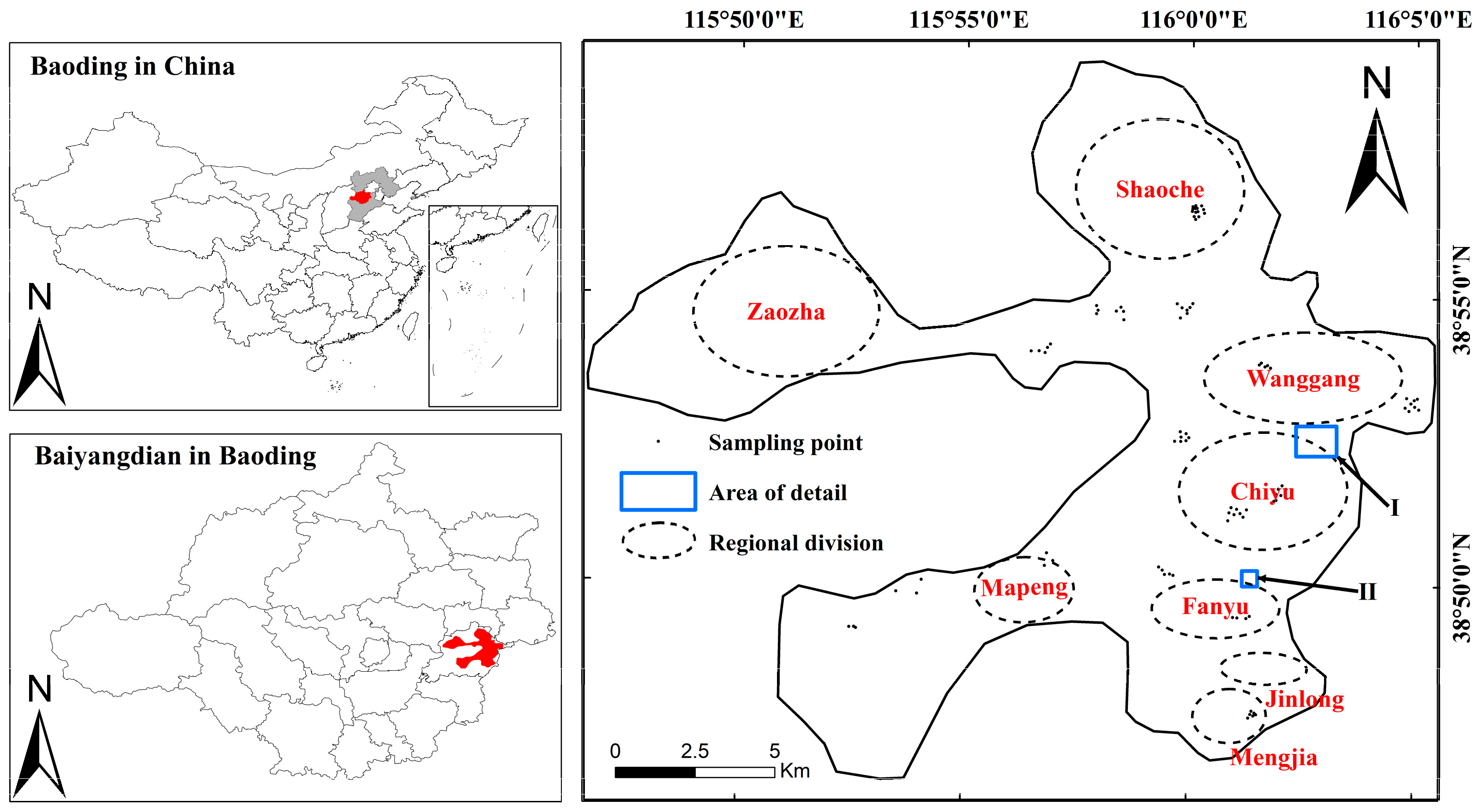
2.1.1. Research Area

Baiyangdian (BYD) is the largest shallow lake in China’s Haihe River Basin, formed in the depression where the Yongding River and Hutuo River alluvial fans meet in front of the Taihang Mountains. We collected 92 water samples from BYD lake, accounting for eight oval-shaped regions (Figure 1), to calculate changes in Chl-a concentrations over time. We also selected two smaller rectangular regions (Figure 1 details areas I and II) to verify the STF results at fine scale, including the water quality correction algorithm and changes of water quality with time.

2.1.2. Data and Processing
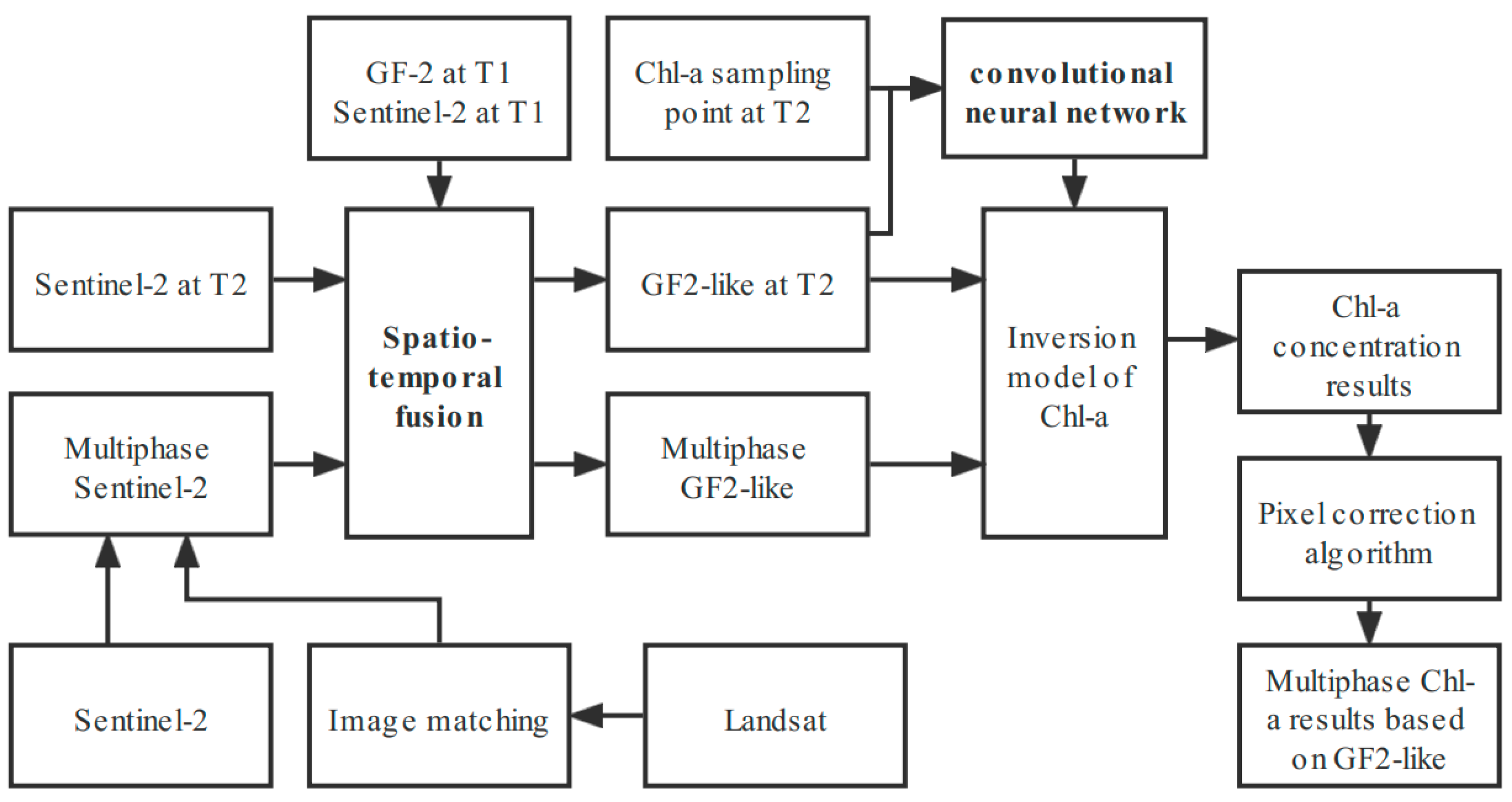
Combined with the field conditions in BYD lake, the growth of phytoplankton varied greatly in August, which helped us to construct the inverse model, and we collected water samples between 21 August and 23 August 2019. We located 92 water quality sampling points using real-time kinematic (RTK) methods and measured their concentrations with EXO multiparameter sonde (a multi-parameter water quality monitor developed by YSI). The GF-2 satellite has a 4-band multispectral sensor with 4 m spatial resolution and a return period of 69 days. This means that there were only two GF-2 images (3 July and 16 August) available from July to September of 2019. GF-2 image preprocessing includes radiation calibration, FLASSH atmospheric correction, and RPC geometric correction. The Sentinel-2 satellite carries a multispectral camera that covers 13 spectral bands with a spatial resolution of 10 m and a temporal resolution of 5 days. Sentinel-2 data are open-source and available from the ESA Copernicus Data Center (Sentinel-2: https://scihub.copernicus.eu/ (accessed on 16 December 2020)). The L2A level product of Sentinel-2 can be used after preprocessing, including orthorectification, geometric precision correction, radiation correction, and atmospheric correction. Sentinel-2 data on 12 July, 27 July, 21 August, and 31 August are used as low-resolution data, Landsat-8 on 1 August and Landsat-7 on 25 August are used as supplements to low-resolution data, and STF is used to generate high spatial resolution data. The generated GF-2-like image on August 16 was compared with the original GF-2 image on 16 August to evaluate the effects of the STF method. The dates and sources for remote sensing imagery analyzed in this study are given in Table 1.

2.2. Methodology

The flow of this paper is shown in Figure 2. In this study, firstly, GF2-like images of the sampling period were generated using spatio-temporal fusion, and a Chl-a inversion model based on a convolutional neural network was established using the sampling points and images as input data. Then, the Sentinel-2 sequence was supplemented using the image-matching algorithm. Spatial and temporal fusion and water quality inversions were performed on multi-period Sentinel-2 data to generate preliminary water quality results. Finally, the corrected GF2-like-based Chl-a concentration time series were generated using the pixel correction algorithm.

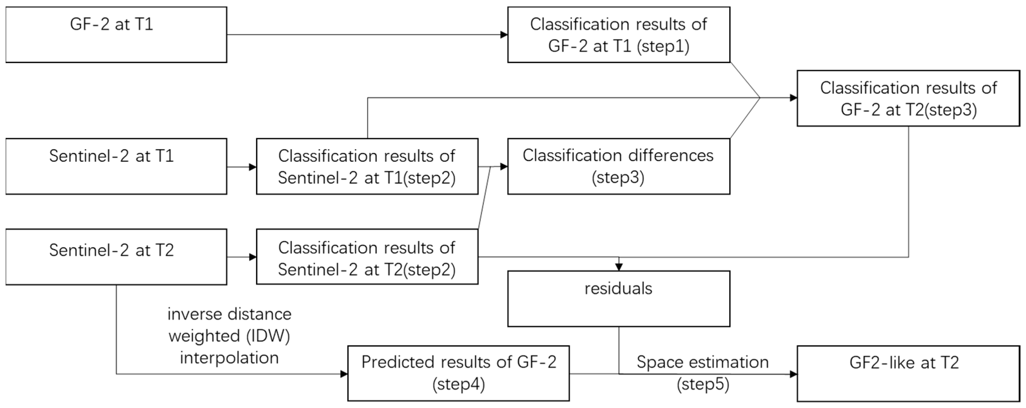
2.2.1. Spatial and Temporal Fusion Method

The production of GF2-like images (GF-2 images generated from contemporaneous Sentinel-2 images via temporal fusion) based on the spatio-temporal fusion method (FSDAF) [33] is divided into 5 steps (Figure 3): (1) classify the GF-2 image at T1 (time 1); (2) classify the Sentinel-2 images of T1 and T2 (time 2), and estimate the time difference between the corresponding classes of the Sentinel-2 images of T1 and T2; (3) predict the GF-2 image classification results at T2 based on the above time differences and calculate the residuals between GF-2 and the Sentinel-2 classification results at the same time; (4) use inverse distance weighted (IDW) interpolation to predict the corresponding GF-2 image based on the Sentinel-2 image at T2; (5) the residual value is assigned to the GF-2 image predicted at time T2 by using the inverse distance weighted interpolation function, and the weight is given by combining the neighborhood information of pixels to correct the accuracy. Finally, the GF2-like image at time T2 is fused and generated.
The calculation process for step 5 is as follows [54]:
Δ R h i g h ( x i j , y i j , b ) = ε h i g h ( x i j , y i j , b ) + Δ R h i g h ( a , b )
R ˜ h i g h 2 ( x i j , y i j , b ) = R h i g h 1 ( x i j , y i j , b ) + k = 1 n [ ω k × Δ R ( x k , y k , b ) ]
where Δ R h i g h ( x i j , y i j , b ) indicates the change of pixel spatial resolution between T1 and T2, ω k is the weight of the k-th similar pixel, ε h i g h ( x i j , y i j , b ) indicates the residuals of the i-th low spatial resolution pixel assigned to the j-th high spatial resolution pixel, and Δ R h i g h ( a , b ) represents the change in low spatial resolution pixels from T1 to T2 for different classifications (a). R ˜ h i g h 2 ( x i j , y i j , b ) indicates the predicted GF2-like data at T2 time, and R h i g h 1 ( x i j , y i j , b ) indicates a high-resolution image input at T1.
Using paired data values (GF-2 data on 3 July, 2019, and Sentinel-2 data on 2 July, 2019) as inputs, we generated four GF2-like images using four Sentinel-2 images on 12 July, 16 August, 21 August, and 25 September. This calculation required about 204 h of computing time using a computer with an Intel Core i7-10700K and 64 G memory.

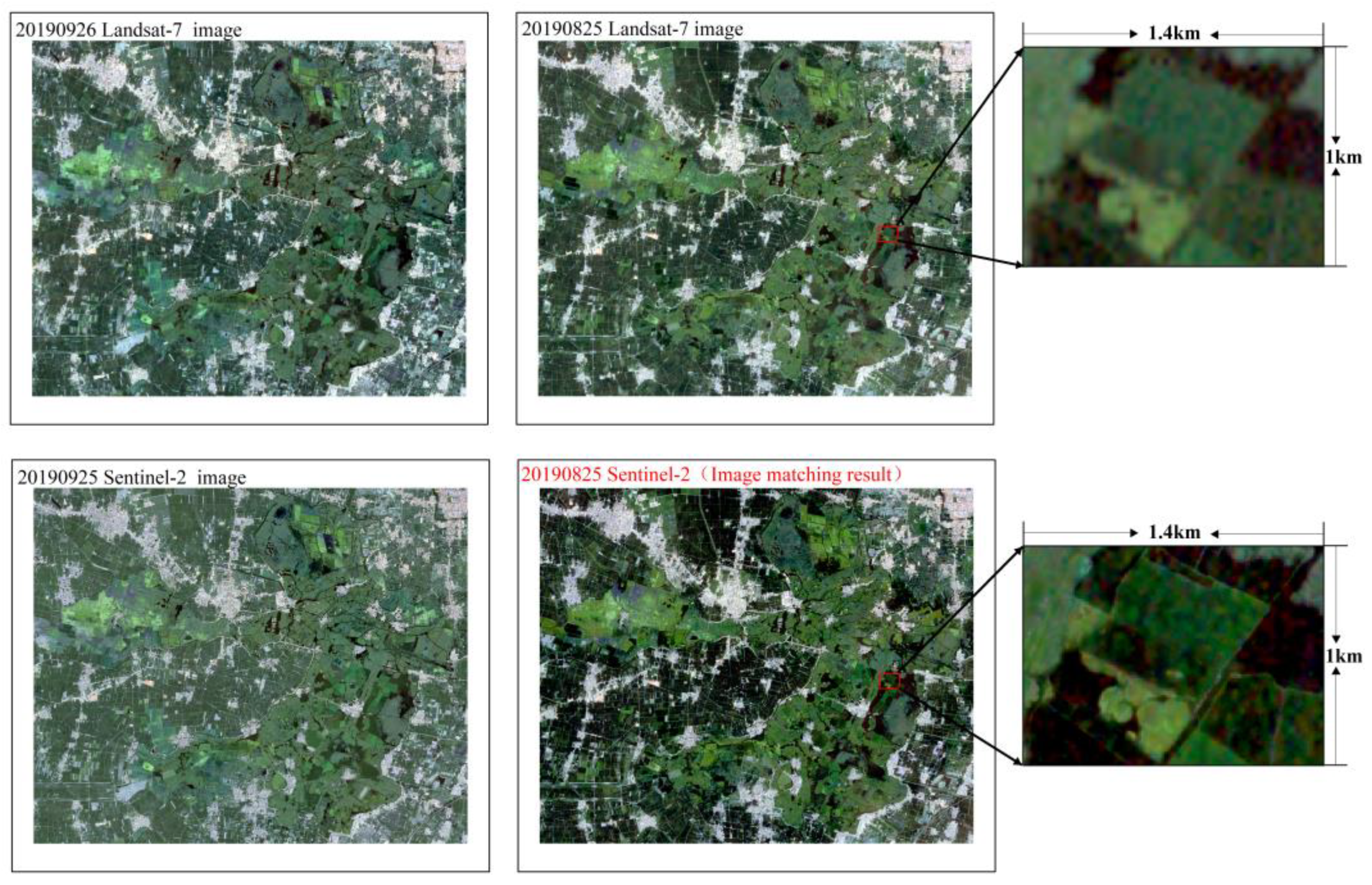
2.2.2. Image-Matching Algorithm

In order to apply more remote sensing data to the inversion model, we propose a simplified version of the data conversion method with reference to the principles of the spatio-temporal fusion algorithm [30,31,32]. We generated Sentinel-2 images using Landsat images. The core idea of this method is to unify the DN value range of the two input data images, calculate the residual of the known image pair, and then superimpose the residual on the image to be converted.
The data conversion algorithm uses Landsat at T1 (M), Landsat at T2 (N), and Sentinel-2 at T1 (X) to generate a Sentinel-2 at T2 (Y), and is divided into the following four steps:
  • All image preprocessing is equally sampled at a 10 m resolution, and the 5th percentile and 95th percentile of each band of the three input images are counted as m 5 , m 95 , n 5 , n 95 , x 5 , and x 95 , respectively. The DN range of the target image X is converted into the original image M:
    X = ( m 95 m 5 ) × ( X x 5 ) / ( x 95 x 5 ) + m 5
  • The residual of X and M is calculated and superimposed on N:
    Y = X M + N
  • To determine the DN range of the target image, calculate the 5th percentile and 95th percentile of the image Y, denoted as y 5 , y 95 :
    y 5 = ( n 5 m 5 ) × k + x 5
    y 95 = ( n 95 m 95 ) × k + x 95
    where k is the conversion factor:
    k = ( x 95 x 5 ) / ( m 95 m 5 )
  • Convert Y to Y:
    Y = ( Y n 5 ) ( y 95 y 5 ) / ( n 95 n 5 ) + y 5
Figure 4 shows the effect of the image matching. We used Landsat-7 of 26 September 2019 and Sentinel-2 of 25 September 2019 as known input pairs to convert Landsat-7 of 25 August 2019 into Sentinel-2 of that day. Similarly, we used Landsat-8 to generate Sentinel-2 of 1 August 2019 to fill in the time series.

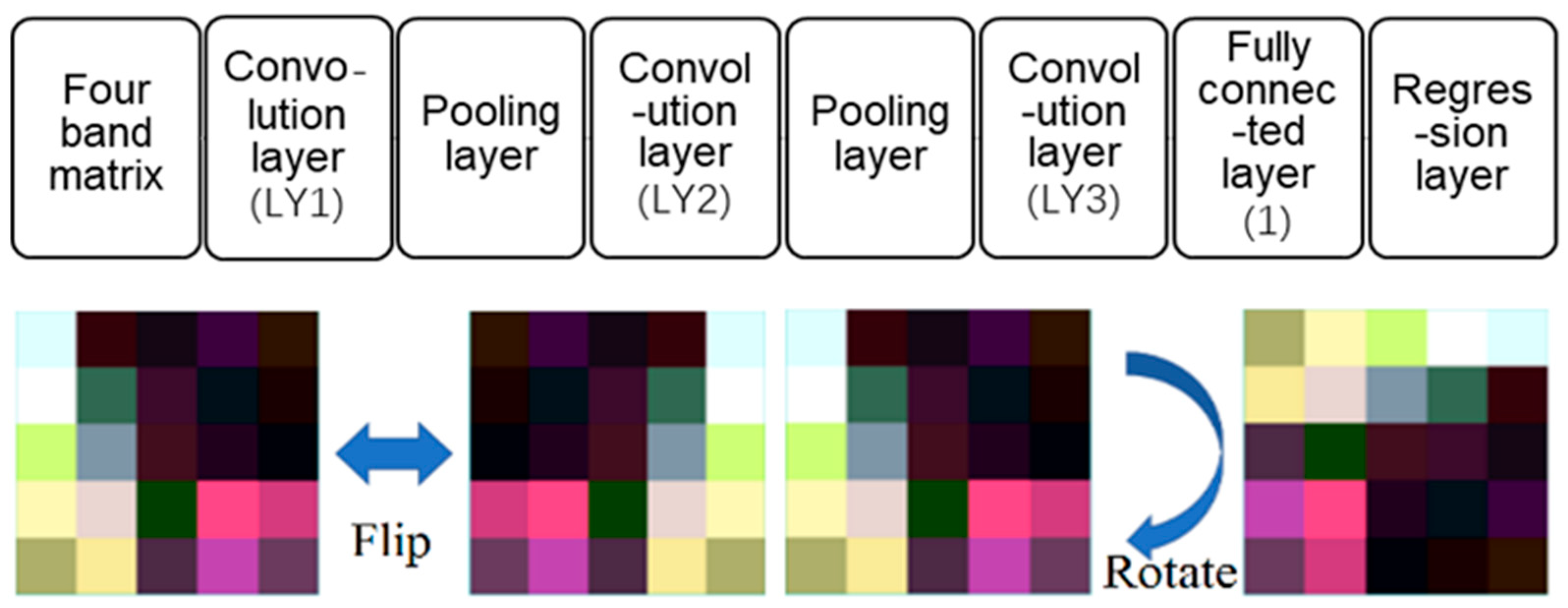
2.2.3. Chl-a Inversion Model Based on CNN

We chose 92 sampling points and their corresponding grid pixels from the GF-2-like image taken on 21 August 2019 as the training input to design a Chl-a inversion model based on CNN [55]. In order to decrease the uncertainties of pixels, 5 × 5 grid pixel matrix blocks were used, and the central pixel corresponds to each sampling point position. Figure 5 shows the structure of the CNN. In this paper, the CNN structure is 4-(LY1-LY2-LY3)-1-1, with four input bands, three hidden layers, one fully connected layer, and one regression layer in that order.
To make the model training more adequate, 92 matrix blocks were extended using a rotation (0°, 90°, 180°, and 270° angles) and flipping of the four rotated blocks. Figure 5 illustrates the method of matrix expansion. The original matrix blocks and their derived expanded matrix blocks correspond to the same water body Chl-a concentrations. The final generated 736 sets of data were used together as a data set for the training of the CNN regression model.
The number of convolutional kernels in the model is incremented to obtain deeper features. To determine the optimal number of convolutional layers, the number of convolutional kernels in the implicit layer, as well as the regularization parameters, the number of iterations, and the learning rate, are adjusted using an iterative algorithm to determine the best combination of parameters to improve the accuracy of the model. Here, 80% of the data was randomly extracted for the training samples and 20% of the data was used for the verification samples for each training session to analyze the accuracy of inversion. In this paper, the R2, RMSE, and average difference (AD) values were calculated to evaluate the true accuracy for the comparison of results.

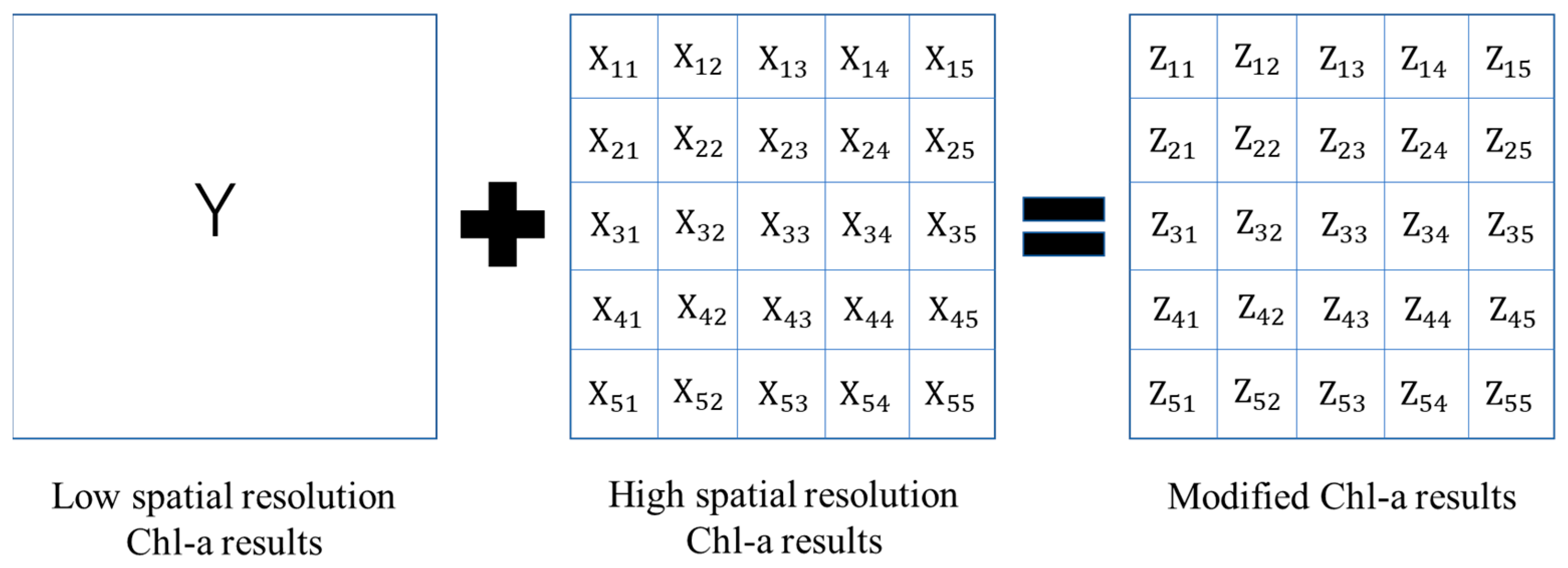
2.2.4. Pixel Correction Algorithm

Due to the fusion error of the spatio-temporal fusion image, the inversion result based on the fusion image (GF2-like) may be different from the inversion result based on the Sentinel-2 image. Therefore, a water quality pixel correction algorithm based on pixel decomposition was proposed. Figure 6 illustrates the correction algorithm for the water quality pixel designed in this study.
The pixel correction algorithm was divided into the following 4 steps:
  • The unified up-sampling of high- and low-resolution Chl-a results of the same period to 2 m resolution is performed, and each set of 5 × 5 low-resolution pixels was homogenized to generate the corresponding confused pixel Y, whose expression is:
    Y = i = 1 , j = 1 5 , 5 W i j 25
    where W i j is the low-resolution image pixel after resampling.
  • The scale factor k is calculated for each pair of corrected pixel, and the expression is:
    k = ( i = 1 , j = 1 5 , 5 X i j 25 ) / Y
    where X i j in the formula is the correction before the image pixel, and Y is the corresponding low-resolution image pixel.
  • Calculate each modified image pixel Z i j of the group according to the scale factor, and the expression is:
    Z i j = X i j k
    where Z i j is the corrected image pixel.

3. Results

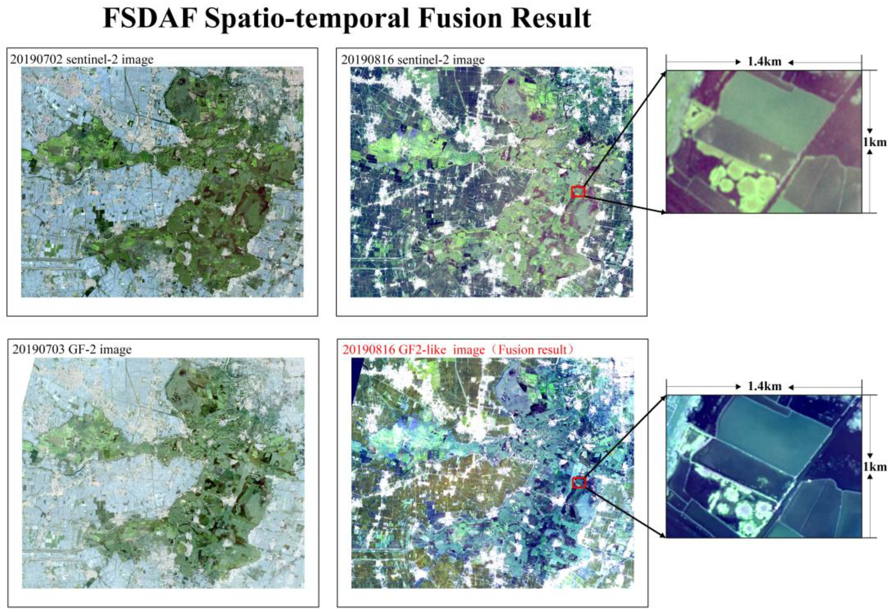
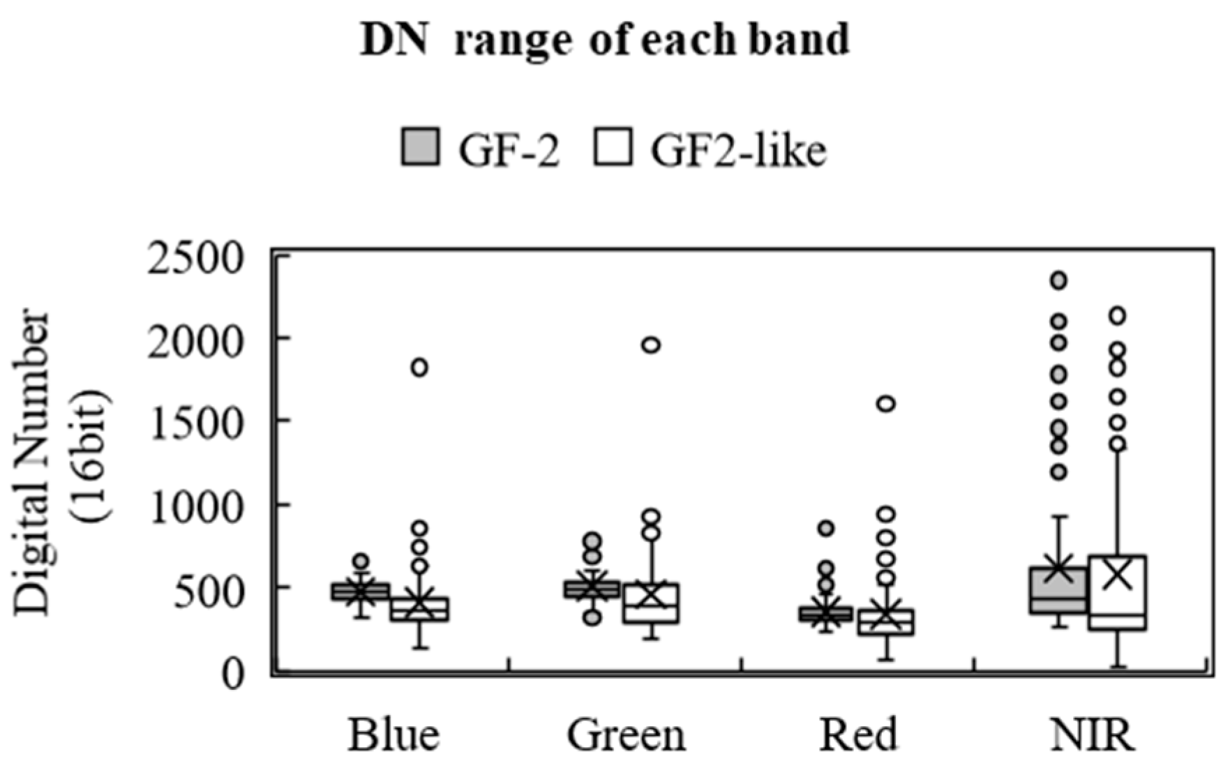
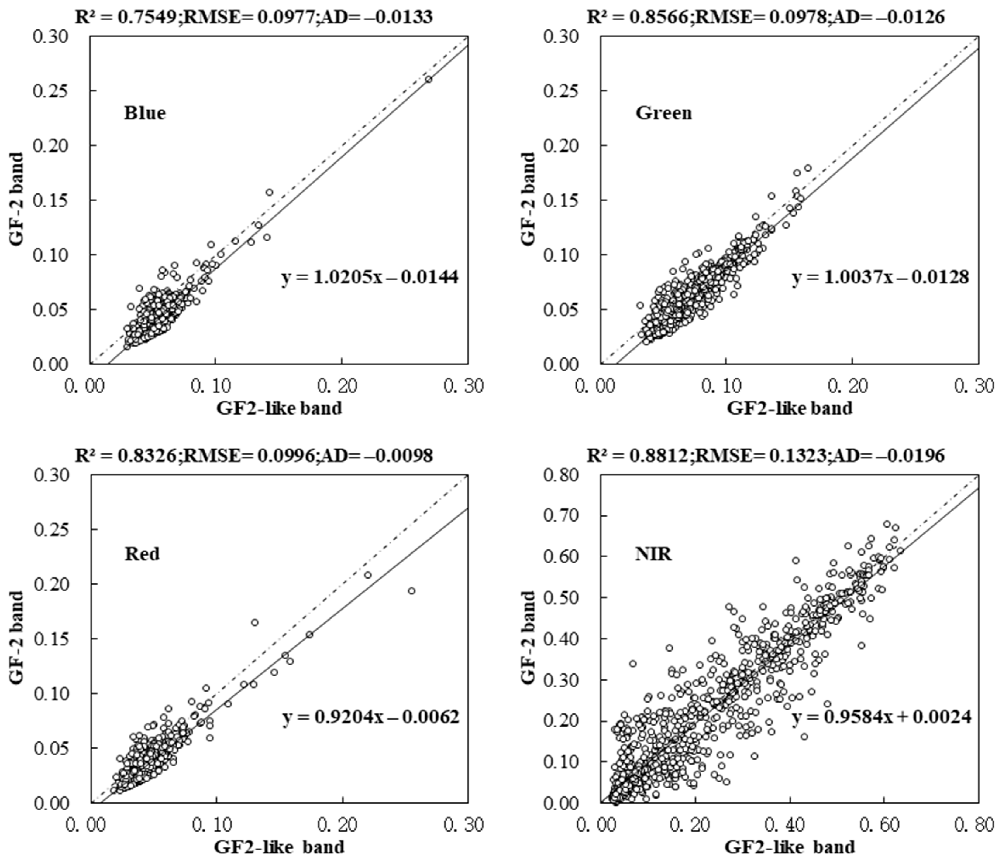
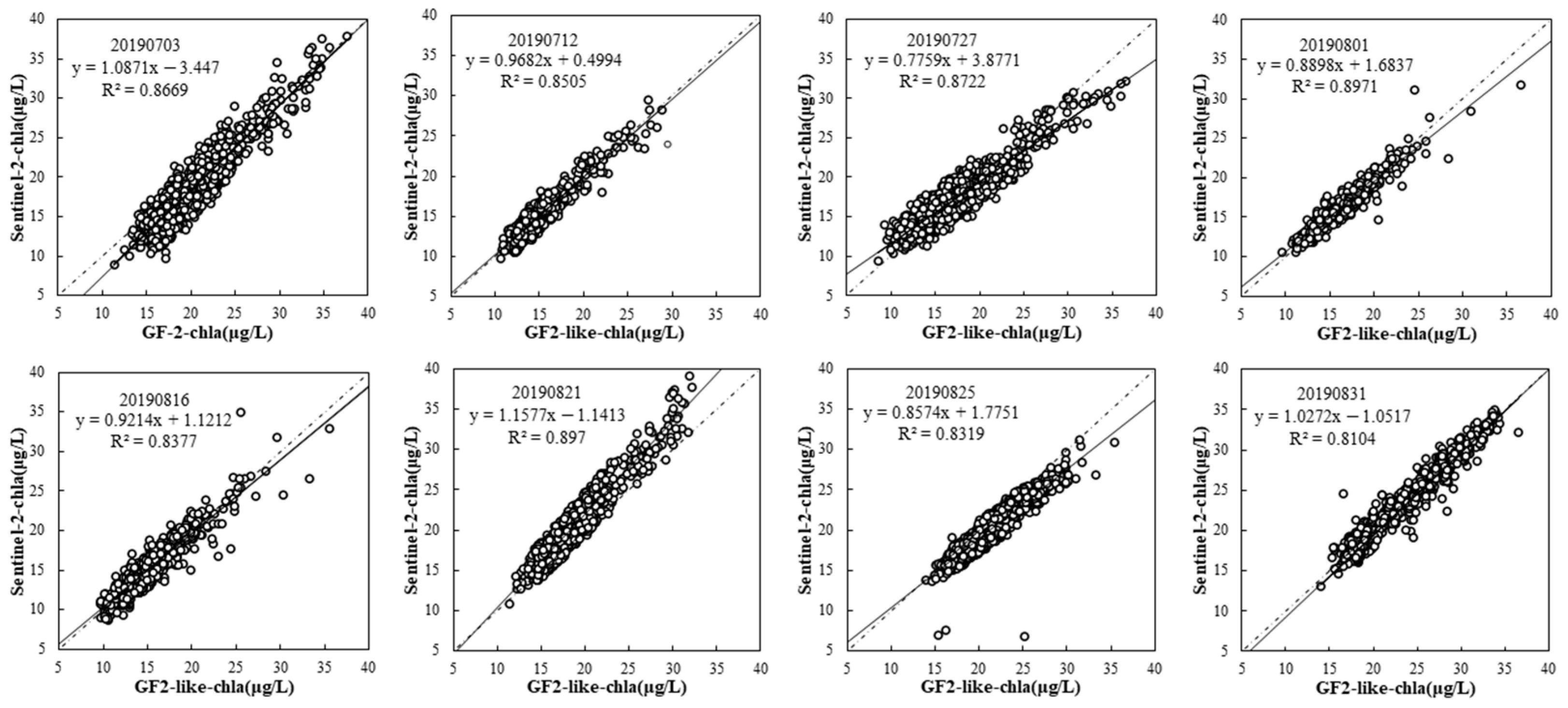
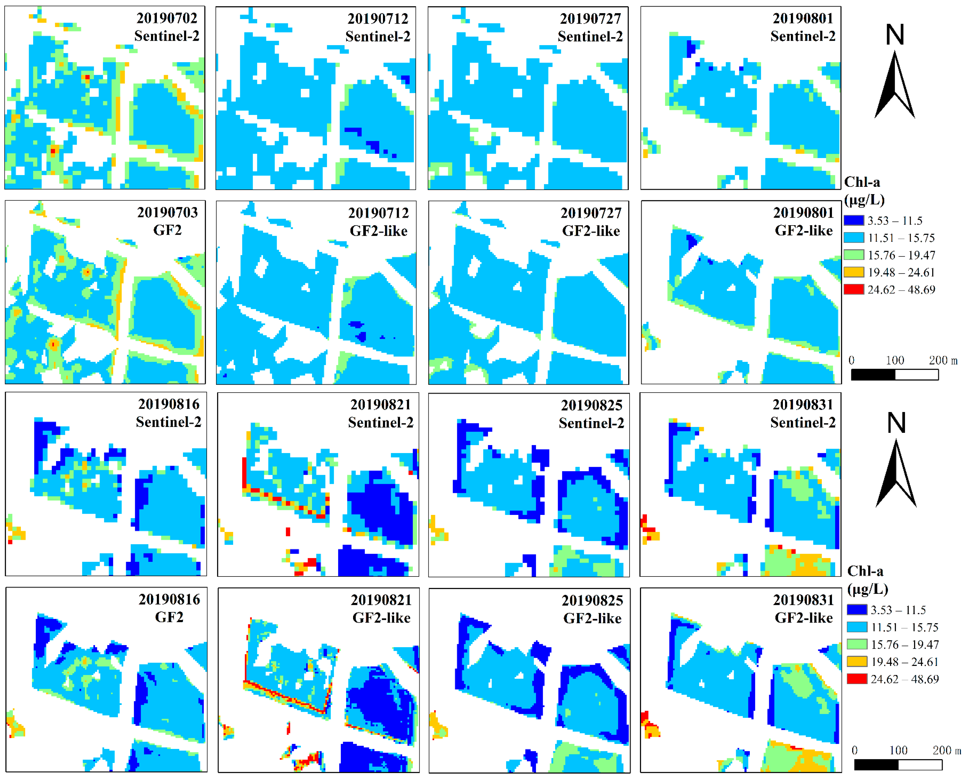
3.1. Spatio-Temporal Fusion Result

Figure 7 shows the spatio-temporal fusion (STF) result for 16 August 2019. The generated GF2-like image indicated a similar spatial distribution compared to the sentinel-2 image. Additionally, the fusion image had a higher spatial resolution with more detailed information, it makes the boundary between the lake and the land clearer. The downside is that the color of the fused image differs from Sentinel-2.
Figure 8 shows the distribution of the 1000 sampled points for the GF-2 and GF-2-like images for each spectral band. We compared the spectral analysis of the GF2-like image with GF-2 images for 16 August 2019 and found that their spectral compositions were similar in the blue, green, and red and NIR band, respectively. Generally, the DN values of the GF2-like image were lower than those of the GF-2 image, and the GF2-like image had more outliers, which were caused by fusion distortion. However, the size distribution trends among the four bands were consistent with the GF-2 image, indicating that the fused data inherited some interrelationships from the original bands.
Figure 9 shows the scatter plot of the DN (digital number) range of different bands based on the GF2-like image and GF-2 image for 16 August 2019. Benefiting from a larger DN range, the correlation in the NIR band was the best with an R2 of 0.8812, and the correlation in the visible band was generally lower than that in the NIR band. The differences between the bands of fused GF2-like images and the GF-2 image were kept roughly within the absolute errors around −0.02. Consistent with the observation of the box line plots, the DN of GF2-like images is slightly lower than that of Sentinel-2.

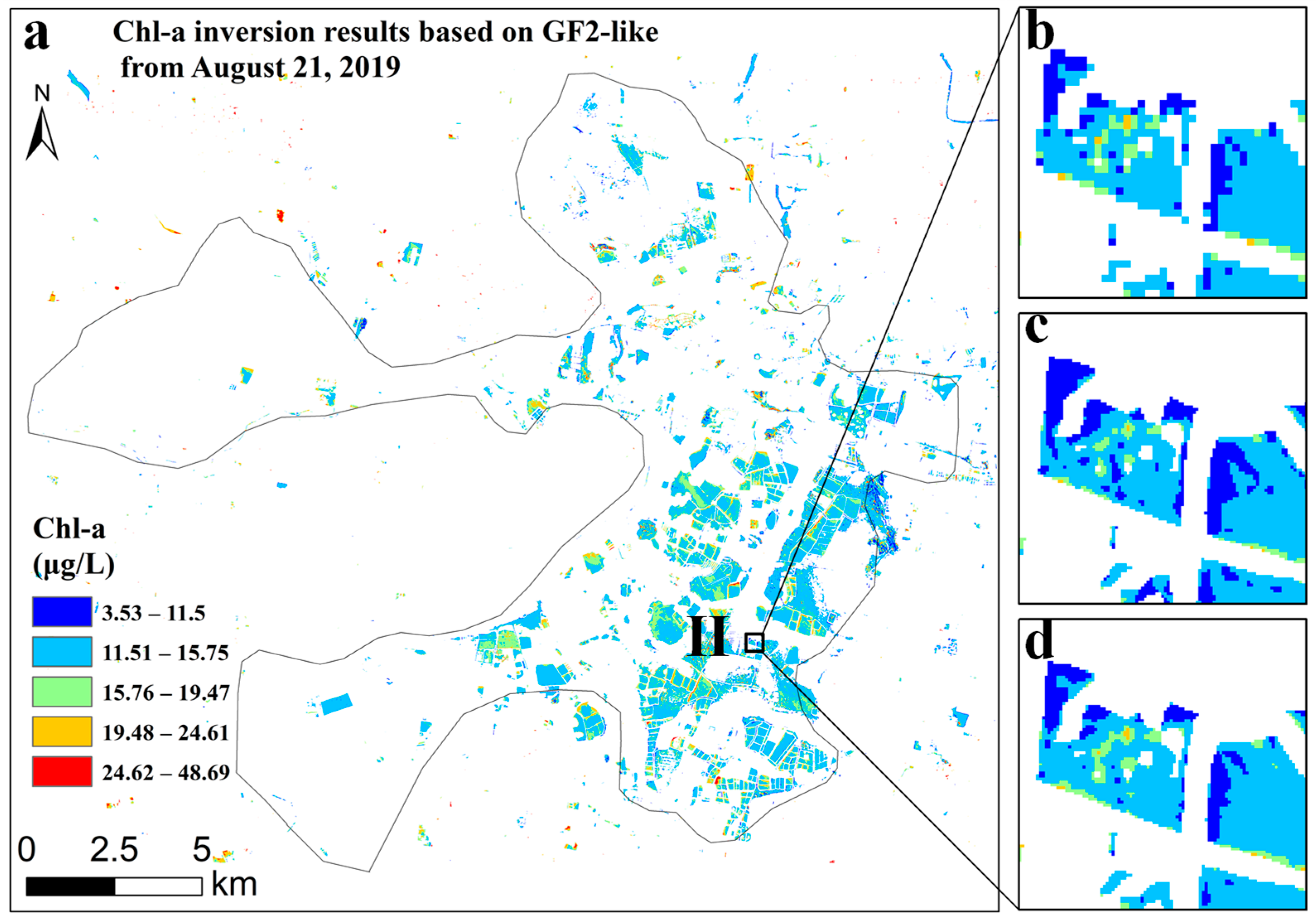
3.2. Chl-a Inversion Results

Figure 10 shows the corresponding correlation level when the training input data are expanded (i.e., when we rotated and flipped the training data to increase the number; see Figure 5) or unexpanded. When the model uses extended data, the average correlation level increases by about 0.1, the correlation degree is generally greater than 0.7, and the highest can reach 0.803.
Figure 11a shows the Chl-a concentration results of BYD lake. The concentration of Chl-a ranged from 3.53 to 48.69 μg/L, and most of the regions are distributed between 3.53 and 19.47 μg/L, indicating that the Chl-a concentration in this region was at a lower level in 21 August 2019. Figure 11b–d shows the detailed Chl-a concentration in region II. The Chl-a inversion results based on the fused images had a higher spatial resolution, but the spatial details were slightly different from those of the low-resolution Chl-a inversion results. After the image pixel correction, the Chl-a inversion results based on the fused image can maintain the same spatial relationship as the low-resolution Chl-a inversion results. The correlation of validation points improved from 0.803 to 0.879, the root-mean-square error decreased from 3.359 to 2.702, and the mean difference decreased from 0.513 to 0.328, which indicated that the image pixel correction was effective.
Figure 12 shows the detailed information, including the image STF result and retrieved Chl-a in regions (I) and (II) for 21 August 2019. The resolution of the GF2-like image was obviously higher than that of the Sentinel-2 image. Comparing the Chl-a results from the Sentinel-2 and GF2-like images, both express well the spatial distribution of Chl-a, while the GF2-like images (Figure 12(a4,b4)) are richer in detail. The images in Figure 12(a4,b4) are smoother than the rough pixel values in Figure 12(a3,b3), providing a more detailed spatial characterization of the Chl-a concentrations. We can clearly see that the darker the water surface color in Figure 12(a1,a2), the higher the Chl-a concentration in Figure 12(a3,a4).

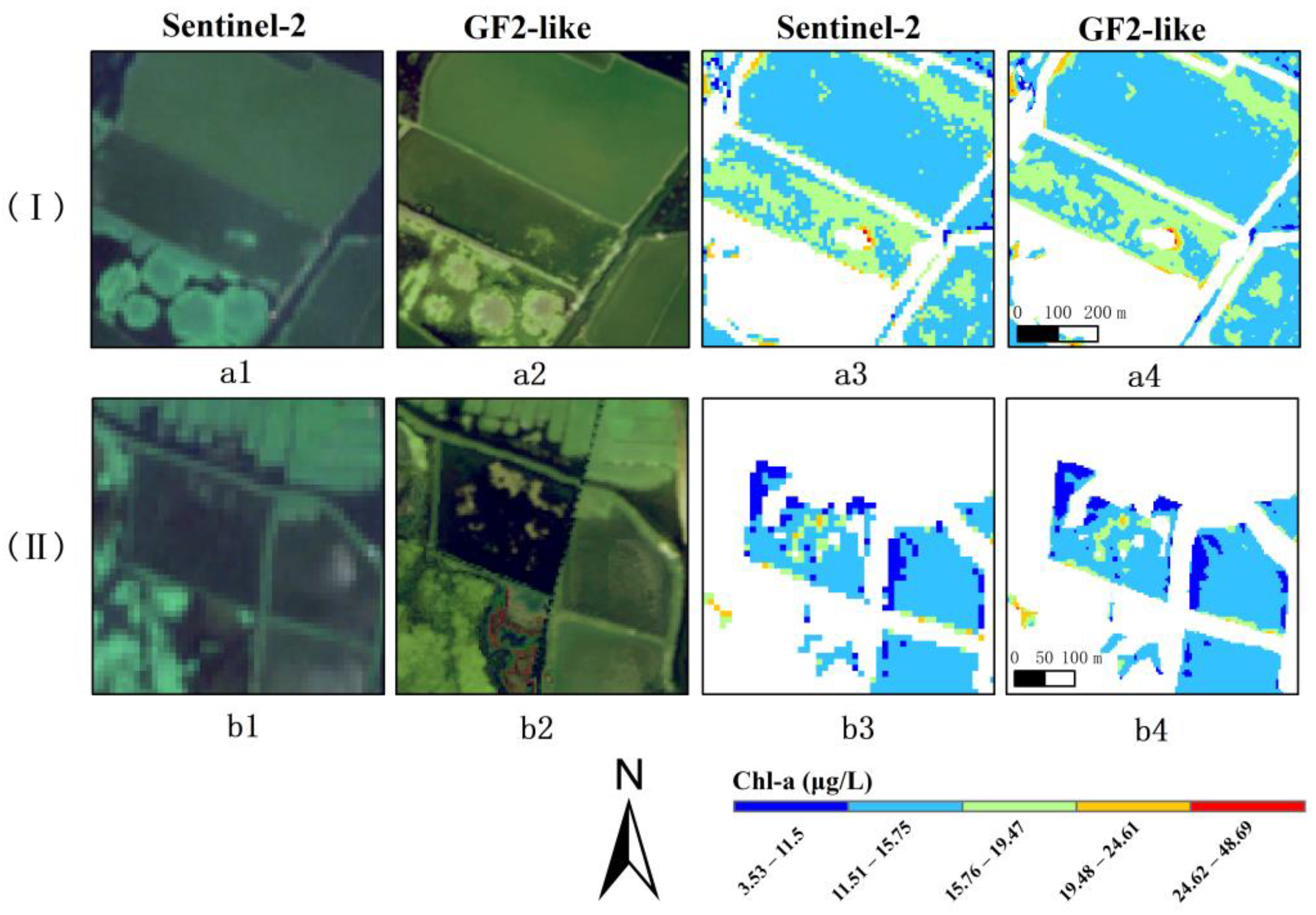
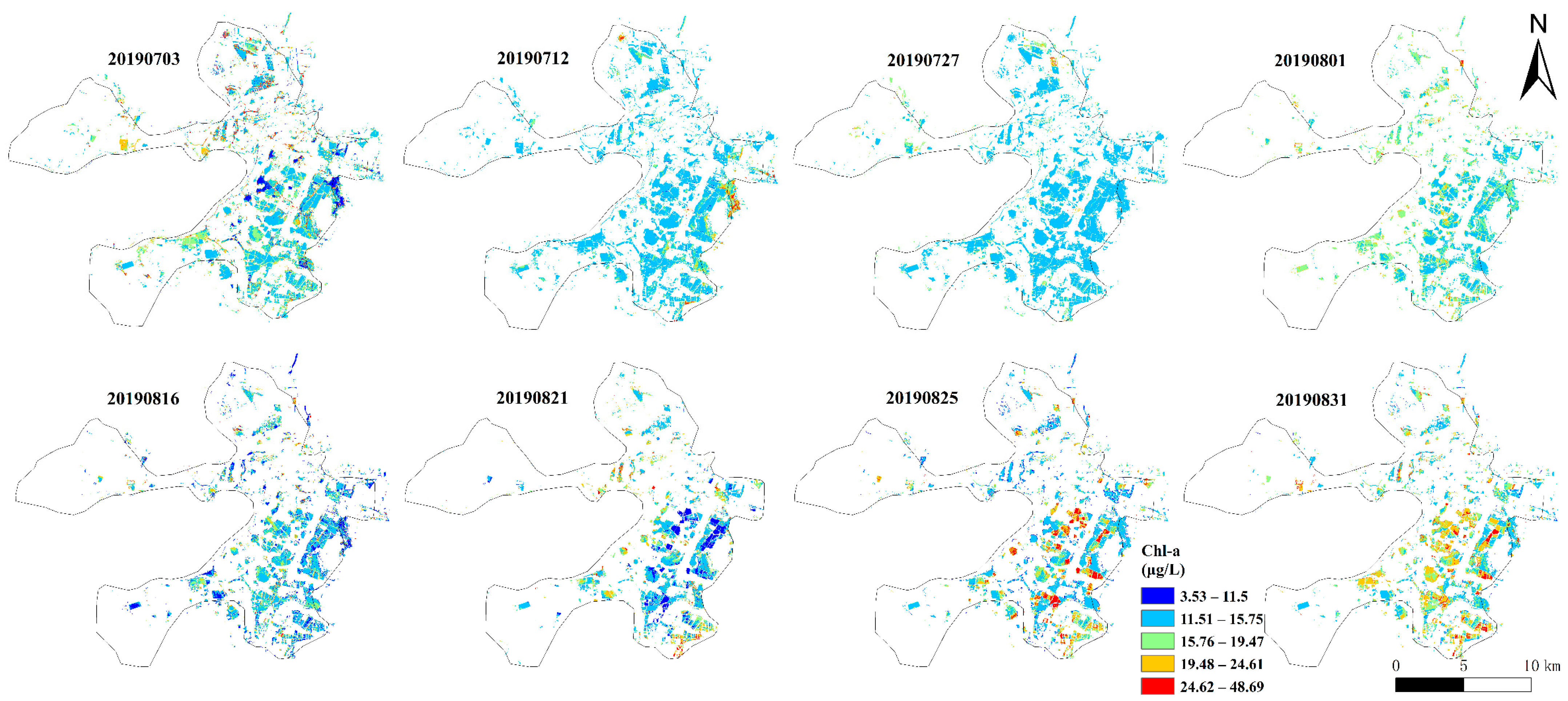
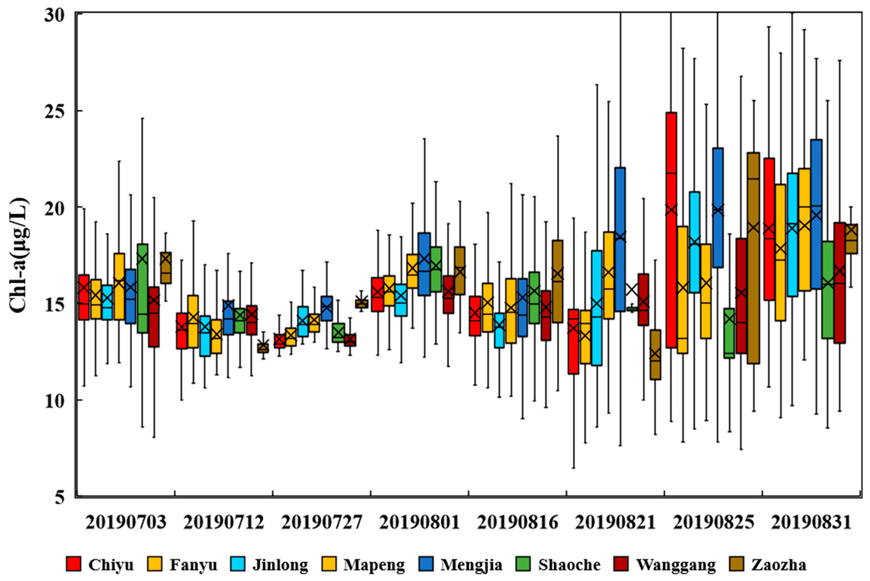
3.3. Comparison of Multi-Period Results

Figure 13 shows the correlation curve for the Chl-a inversion results of the Sentinel-2 images and GF2-like images. It can be seen that all inversion results had a higher correlation (R2 > 0.81) with good reliability. The difference between STF images and low-resolution images ranges from 0 to 6 μg/L. The sample points are shifted to the upper right corner on 21 August, 25 August, and 31 August, indicating a significant increase in Chl-a during this period.
Figure 14 clearly represents the difference in spatial detail between the Chl-a inversion results of multi-phase Sentinel-2 and GF-2 images, and we have chosen region II for comparison. On this time series, we can see an overall increasing trend of Chl-a concentrations over time, with a large variation in phytoplankton growth during August, and an opposite increasing trend from 21 August to 25 August. The Chl-a concentrations in some periods deviated from the overall pattern, for example, the concentrations on 2 July and 21 August were higher than the normal trend. The overall spatial distribution of GF2-like images was in good agreement with that of Sentinel-2, while it was richer in spatial details. However, there are still local differences, although they are few.
Figure 15 shows the water quality results of BYD lake on 2 July, 12 July, 27 July, 1 August, 16 August, 21 August, 25 August, and 31 August of 2019. Chl-a concentrations were retrieved using the trained neural network model and pixel correction algorithm. From July to August, Chl-a concentrations decreased and then increased, remaining below 20 μg/L in most areas. On 31 August, Chl-a concentrations reached 20 μg/L in most areas. There were some areas with small changes in chlorophyll concentration over time, while there were some adjacent areas with opposite trends in chlorophyll concentrations. The periods with large geographic differences in Chl-a concentrations were 3 July, 21 August, 25 August, and 31 August, with a relatively stable growth trend during July and a faster growth change during August. In addition, we found that the change trend of the inversion results of Sentinel-2 data generated by Landsat is consistent with that of real Sentinel-2 data, indicating that the data supplement is feasible.
Figure 16 shows the comparison of Chl-a concentrations in the eight areas of BYD lake (Figure 1). We plotted the mean and range of 1000 points from each area for eight consecutive dates. We found that there was a slight decrease in Chl-a concentration in BYD lake during July, and the regional differences gradually decreased. During August, Chl-a concentrations increased at different degrees in all regions, and the range of values in the region became wider, indicating that there was a great variation in algal growth in August, and algal outbreaks occurred locally in BYD lake. Overall, the Chl-a concentration in BYD lake was greater in August than in July, with the highest value greater than 30 μg/L throughout August and a high degree of eutrophication, and the lowest Chl-a concentration in late July, with concentrations ranging from 10 to 15 μg/L.

4. Discussion

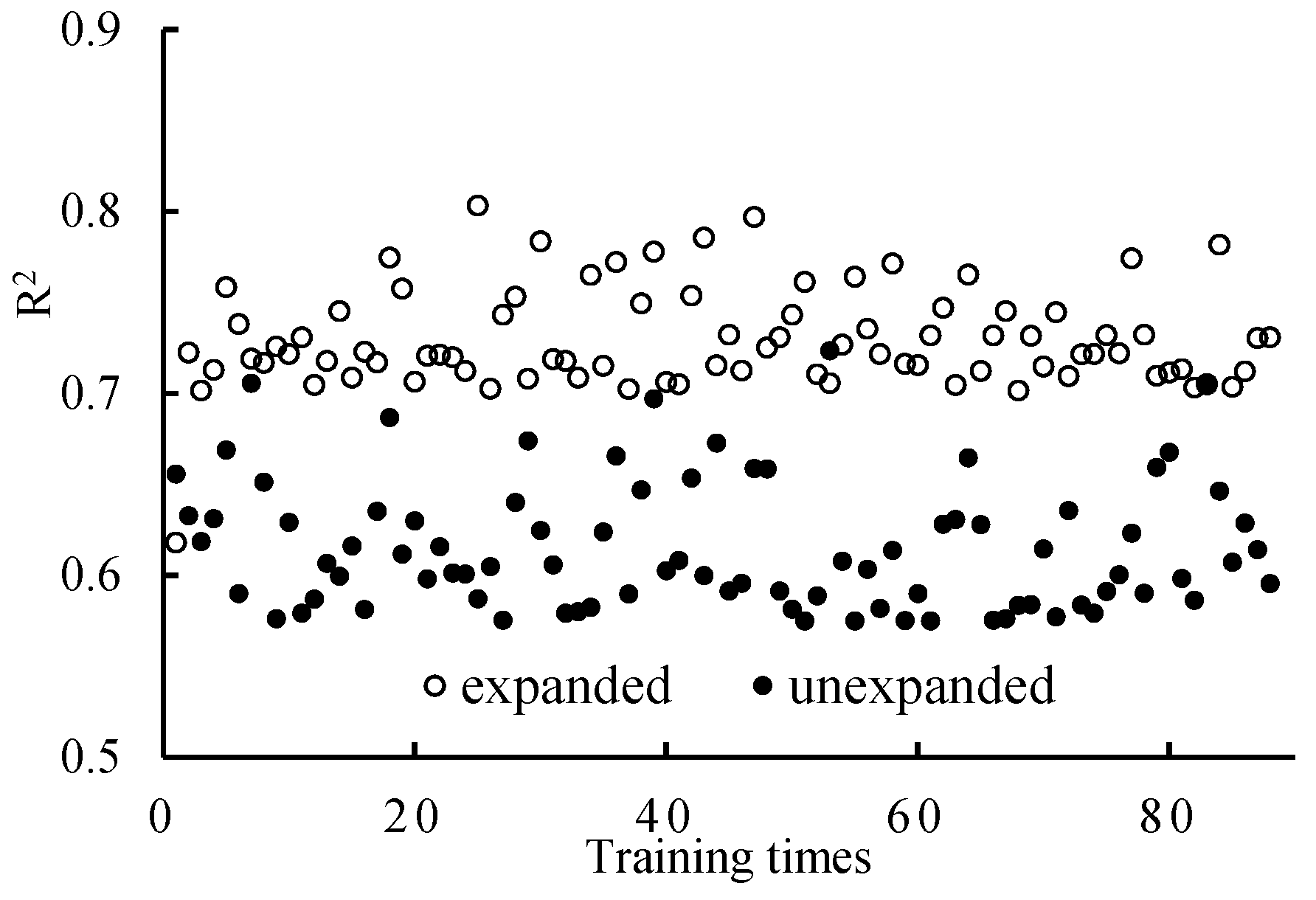
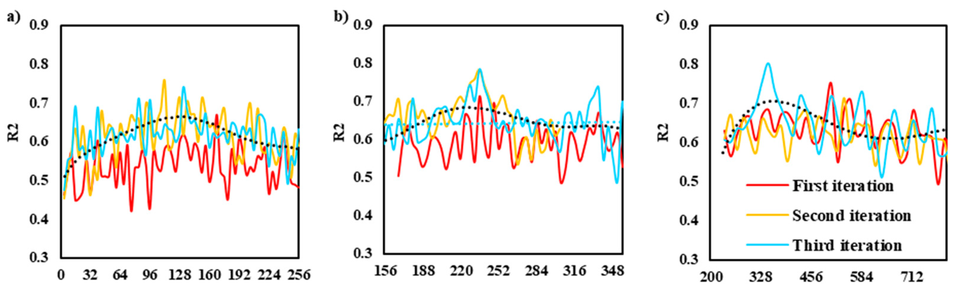
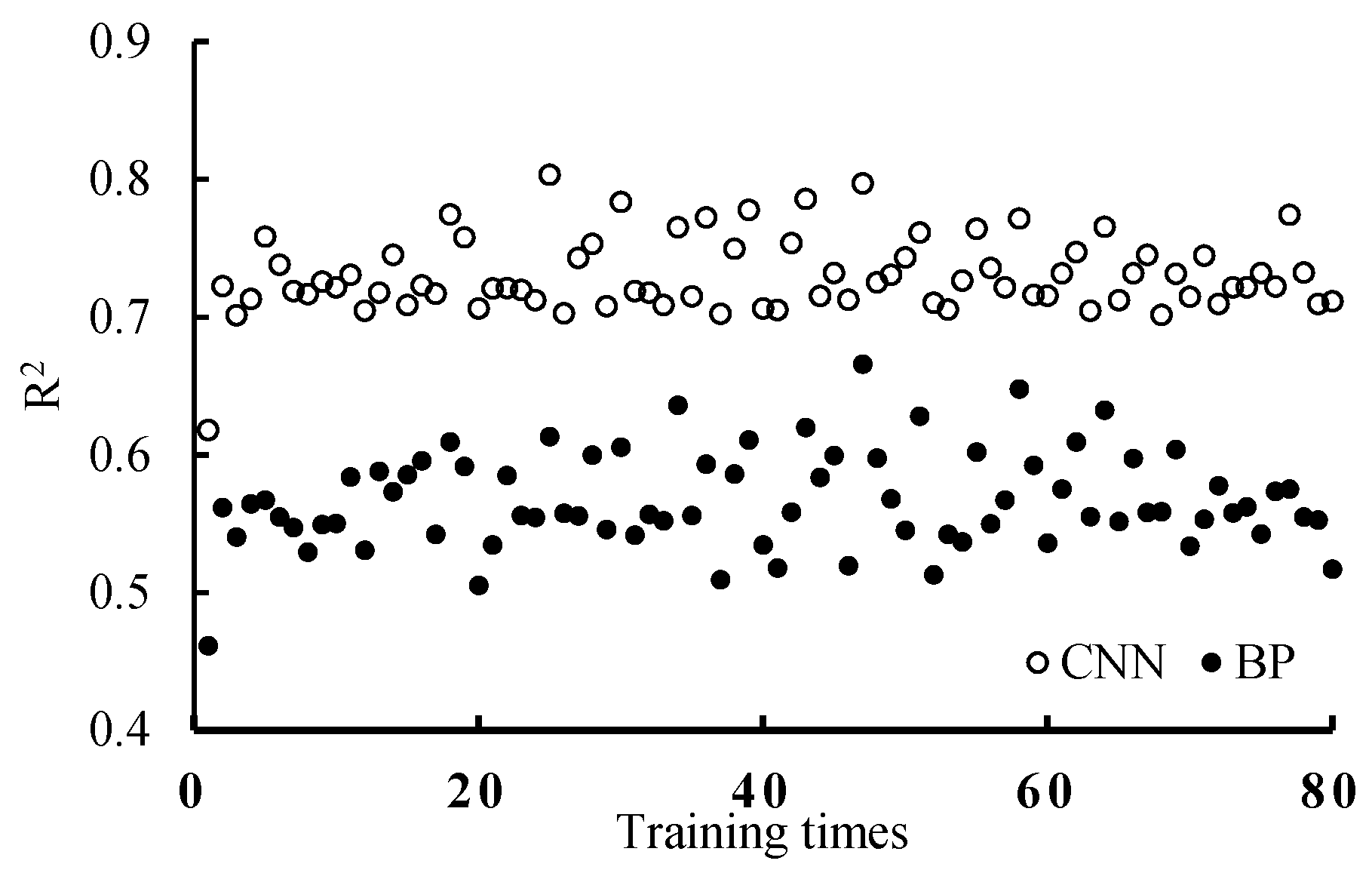
4.1. Sensitivity of Chl-a Inversion Model Based on CNN Structure

Many scholars have tried to construct water quality inversion models with CNN and achieved good results, for example, Maier et al. used a 1D CNN for Chl-a simulation training [56], and Aptoula et al. used a 2D CNN and a 3D CNN for Chl-a simulation training, where the R2 reached 0.93 [57]. We used a 2D CNN for training in our experiments, and Figure 17 shows the effect of the number of convolutional kernels per layer on the effect of the model, and the accuracy curves for the first three iterations are plotted in the figure. We found that as the number of iterations increased, the accuracy of the first and second layers improved significantly, while the accuracy of the third layer improved less. Pu et al. concluded that the optimal number of convolutional kernel layers for inverse water quality grading in convolutional neural networks is two to seven layers [55], which is consistent with our observation. We finally determined the CNN structure as 4-(136-236-340)-1-1, the learning rate was set to 0.001, the number of iterations was set to 100, and the regularization parameter was set to 0.001. Its correlation coefficient R2 reached 0.803. This accuracy level is normal because the wide spectral bandwidth of GF-2 images weakened the spectral features [58]. We trained with Sentinel-2 images under CNN and found that its best correlation coefficient R2 reached 0.887, which is similar to the accuracy level of the related study [59].

4.2. Advantages

The CNN-based Chl-a inversion model can effectively reflect the rich spatial information of the fused images and obtain high spatial resolution Chl-a inversion results [60]. Figure 18 shows the correlation level between BP (backpropagation) and the CNN, and the accuracy of the CNN is higher than BP when there are enough samples [61]. The CNN takes full advantage of the high-resolution features of the fused images and reduces the unexpected errors caused by the small field of view of traditional inversion methods [38,62].
In pursuit of data reliability and accessibility, scholars have often used open-source data such as Sentinel-2 (10 m), Landsat series (15 m), and Modis (500 m) for remote sensing inversion [63,64,65]. Lin et al. found that the area of BYD lake in flood season can reach 290 km2 [66], and it is difficult to achieve remote sensing inversion with a large range, a high frequency, and a high spatial resolution. Yang et al. used STF for the inversion of surface temperature in Zhengzhou City [54], and we applied STF to the inversion of Chl-a with the same good results. A similar study was conducted by Liu et al. who used Sentinel-2, Landsat-8, and Modis for spatio-temporal fusion and SPM (suspended particulate matter) inversion [67]. Compared to this author, we proposed image-matching and pixel correction algorithms to further complement the time series and improve the accuracy of the inversion. Related data show that Baiyangdian has abundant precipitation during the flood season from July to September [68], and some scholars [69] found that precipitation can cause the short-term growth of Chl-a, which is consistent with our observation.

4.3. Limitations

The combination of STF and CNN has been well applied in Chl-a inversion. This method can also be applied to any area with sufficient data for water quality sampling points, but it still has some limitations. For example, our study has only 92 sample points; in the study of Aptoula, E. et al., the number of sample points reached 320 and their R2 was higher than ours [57]. Although we increased the sample points via data expansion, more measured sample points could lead to higher accuracy [70]. Limited by the current sensor development, there are fewer satellites with both high spatial resolution and good spectral characteristics [71]. Therefore, in order to obtain better accuracy for water quality inversion, fusion experiments with hyperspectral satellites and UAVs can be further investigated [58,72]. Since many scholars have improved the fusion algorithm, further research can be conducted using better STF methods, such as EFSDAF [73].

5. Conclusions

In this study, we developed and verified an inversion model of Chl-a concentration based on CNN with fused high spatial and temporal resolution images, and analyzed the variation of Chl-a concentrations in Baiyangdian from July 2019 to September 2019. We found that CNN can reflect the spatial information of spatio-temporal fused images more effectively. In order to supplement the time series, a data conversion method is proposed to convert the Landsat images and supplement the Sentinel-2 images. To overcome the distortion of the fusion result, a pixel correction method based on image element decomposition was proposed to correct the inversion results of GF2-like images. The measured Chl-a and retrieved Chl-a had a high correlation (R2 = 0.803), and the correlation R2 increased to 0.879 after pixel correction. The Chl-a concentrations in BYD lake decreased and then increased from July to August and reached the maximum value on 31 August. This study shows that the proposed inversion model can reflect the spatial and temporal distribution of water quality parameters more accurately, and this method can also be applied to any area with sufficient water quality sampling point data.

Author Contributions

Conceptualization, H.Y. and Y.D.; methodology, Y.D.; validation, H.Z.; formal analysis, Y.D.; investigation, H.Z. and F.C.; resources, F.C.; writing—original draft preparation, Y.D.; writing—review and editing, H.Y. and H.Z.; supervision, H.Y.; project administration, H.Y.; funding acquisition, H.Y. All authors have read and agreed to the published version of the manuscript.

Funding

This research was supported by the National Key R&D Program of China (Grant No. 2018YFC0406505). Science and technology project of Henan Province (Grant No. 142102210069). Key scientific research projects of Henan colleges and universities (Grant No. 19A170014).

Institutional Review Board Statement

Not applicable.

Informed Consent Statement

Not applicable.

Data Availability Statement

Some data, models, or code that support the findings of this study are available from the corresponding author upon reasonable request.

Acknowledgments

These authors would like to thank the European Space Agency for providing us with the Sentinel-2 data (https://scihub.copernicus.eu (accessed on 16 December 2020)).

Conflicts of Interest

The authors declare that they have no known competing financial interest or personal relationships that could have appeared to influence the work reported in this paper.

References

  1. Galgani, L.; Loiselle, S.A. Plastic pollution impacts on marine carbon biogeochemistry. Environ. Pollut. 2021, 268, 115598. [Google Scholar] [CrossRef] [PubMed]
  2. Olaka, L.A.; Ogutu, J.O.; Said, M.Y.; Oludhe, C. Projected Climatic and Hydrologic Changes to Lake Victoria Basin Rivers under Three RCP Emission Scenarios for 2015–2100 and Impacts on the Water Sector. Water 2019, 11, 1449. [Google Scholar] [CrossRef] [Green Version]
  3. Fazi, S.; Amalfitano, S.; Venturi, S.; Pacini, N.; Vazquez, E.; Olaka, L.A.; Tassi, F.; Crognale, S.; Herzsprung, P.; Lechtenfeld, O.J.; et al. High concentrations of dissolved biogenic methane associated with cyanobacterial blooms in East African lake surface water. Commun. Biol. 2021, 4, 845. [Google Scholar] [CrossRef] [PubMed]
  4. Moss, B. Cogs in the endless machine: Lakes, climate change and nutrient cycles: A review. Sci. Total Environ. 2012, 434, 130–142. [Google Scholar] [CrossRef] [PubMed]
  5. Yin, D.; Wang, L.; Zhu, Z.; Clark, S.S.; Cao, Y.; Besek, J.; Dai, N. Water quality related to Conservation Reserve Program (CRP) and cropland areas: Evidence from multi-temporal remote sensing. Int. J. Appl. Earth Obs. Geoinf. 2021, 96, 102272. [Google Scholar] [CrossRef]
  6. Schaeffer, B.A.; Schaeffer, K.G.; Keith, D.; Lunetta, R.S.; Conmy, R.; Gould, R.W. Barriers to adopting satellite remote sensing for water quality management. Int. J. Remote Sens. 2013, 34, 7534–7544. [Google Scholar] [CrossRef]
  7. Malahlela, O.E.; Iop. Spatio-temporal assessment of inland surface water quality using remote sensing data in the wake of changing climate. In Proceedings of the Third International Conference on Energy Engineering and Environmental Protection, Sanya, China, 19–21 November 2018; Volume 227. [Google Scholar]
  8. Pinardi, M.; Villa, P.; Free, G.; Giardino, C.; Bresciani, M. Evolution of Native and Alien Macrophytes in a Fluvial-wetland System Using Long-term Satellite Data. Wetlands 2021, 41, 16. [Google Scholar] [CrossRef]
  9. Villa, P.; Bresciani, M.; Bolpagni, R.; Braga, F.; Bellingeri, D.; Giardino, C. Impact of upstream landslide on perialpine lake ecosystem: An assessment using multi-temporal satellite data. Sci. Total Environ. 2020, 720, 137627. [Google Scholar] [CrossRef]
  10. Gupana, R.S.; Odermatt, D.; Cesana, I.; Giardino, C.; Nedbal, L.; Damm, A. Remote sensing of sun-induced chlorophyll-a fluorescence in inland and coastal waters: Current state and future prospects. Remote Sens. Environ. 2021, 262, 112482. [Google Scholar] [CrossRef]
  11. Yin, Z.; Li, J.; Liu, Y.; Xie, Y.; Zhang, F.; Wang, S.; Sun, X.; Zhang, B. Water clarity changes in Lake Taihu over 36 years based on Landsat TM and OLI observations. Int. J. Appl. Earth Obs. Geoinf. 2021, 102, 102457. [Google Scholar] [CrossRef]
  12. Randhawa, S.; Guruprasad, R.B.; Balivada, S.R.; Hirani, P.; Guha, S. Bluewater Eye: Using satellite as a low cost water pollution sensor: Analytics for deriving long term pollution insights based on mapping water turbidity. In Proceedings of the Remote Sensing for Agriculture, Ecosystems, and Hydrology Xx, Berlin, Germany, 10–13 September 2019; Volume 10783. [Google Scholar]
  13. Tsapanou, A.; Oikonomou, E.; Drakopoulos, P.; Poulos, S.; Sylaios, G. Coupling remote sensing data with in-situ optical measurements to estimate suspended particulate matter under the Evros river influence (North-East Aegean sea, Greece). Int. J. Remote Sens. 2020, 41, 2062–2080. [Google Scholar] [CrossRef]
  14. Campbell, G.; Phinn, S.R.; Dekker, A.G.; Brando, V.E. Remote sensing of water quality in an Australian tropical freshwater impoundment using matrix inversion and MERIS images. Remote Sens. Environ. 2011, 115, 2402–2414. [Google Scholar] [CrossRef] [Green Version]
  15. Yang, M.M.; Ishizaka, J.; Goes, J.I.; Gomes, H.d.R.; Maúre, E.d.R.; Hayashi, M.; Katano, T.; Fujii, N.; Saitoh, K.; Mine, T.; et al. Improved MODIS-Aqua Chlorophyll-a Retrievals in the Turbid Semi-Enclosed Ariake Bay, Japan. Remote Sens. 2018, 10, 1335. [Google Scholar] [CrossRef] [Green Version]
  16. Qun’ou, J.; Lidan, X.; Siyang, S.; Meilin, W.; Huijie, X. Retrieval model for total nitrogen concentration based on UAV hyper spectral remote sensing data and machine learning algorithms—A case study in the Miyun Reservoir, China. Ecol. Indic. 2021, 124, 107356. [Google Scholar] [CrossRef]
  17. Kuhn, C.; Valerio, A.d.M.; Ward, N.; Loken, L.; Sawakuchi, H.O.; Kampel, M.; Richey, J.; Stadler, P.; Crawford, J.; Striegl, R.; et al. Performance of Landsat-8 and Sentinel-2 surface reflectance products for river remote sensing retrievals of chlorophyll-a and turbidity. Remote Sens. Environ. 2019, 224, 104–118. [Google Scholar] [CrossRef] [Green Version]
  18. Wu, D.; Yu, W.; Xie, T. Application of GF-2 Satellite Data for Monitoring Organic Pollution Delivered to Water Bodies in the Guangdong-Hong Kong-Macao Greater Bay Area. Trop. Geogr. 2020, 40, 675–683. [Google Scholar]
  19. Jiang, G.; Loiselle, S.A.; Yang, D.; Ma, R.; Su, W.; Gao, C. Remote estimation of chlorophyll a concentrations over a wide range of optical conditions based on water classification from VIIRS observations. Remote Sens. Environ. 2020, 241, 111735. [Google Scholar] [CrossRef]
  20. Ekercin, S. Water Quality Retrievals from High Resolution Ikonos Multispectral Imagery: A Case Study in Istanbul, Turkey. Water Air Soil Pollut. 2007, 183, 239–251. [Google Scholar] [CrossRef]
  21. Bramich, J.M.; Bolch, C.J.; Fischer, A.M. Evaluation of atmospheric correction and high-resolution processing on SeaDAS-derived chlorophyll-a: An example from mid-latitude mesotrophic waters. Int. J. Remote Sens. 2018, 39, 2119–2138. [Google Scholar] [CrossRef]
  22. Andrzej Urbanski, J.; Wochna, A.; Bubak, I.; Grzybowski, W.; Lukawska-Matuszewska, K.; Łącka, M.; Śliwińska, S.; Wojtasiewicz, B.; Zajączkowski, M. Application of Landsat 8 imagery to regional-scale assessment of lake water quality. Int. J. Appl. Earth Obs. Geoinf. 2016, 51, 28–36. [Google Scholar] [CrossRef]
  23. Zhang, C.; Long, D.; Zhang, Y.; Anderson, M.C.; Kustas, W.P.; Yang, Y. A decadal (2008–2017) daily evapotranspiration data set of 1 km spatial resolution and spatial completeness across the North China Plain using TSEB and data fusion. Remote Sens. Environ. 2021, 262, 112519. [Google Scholar] [CrossRef]
  24. Cao, Z.; Ma, R.; Duan, H.; Xue, K.; Shen, M. Effect of Satellite Temporal Resolution on Long-Term Suspended Particulate Matter in Inland Lakes. Remote Sens. 2019, 11, 2785. [Google Scholar] [CrossRef] [Green Version]
  25. Johnson, M.C.; Reich, B.J.; Gray, J.M. Multisensor fusion of remotely sensed vegetation indices using space-time dynamic linear models. J. R. Stat. Soc. C-Appl. 2021, 70, 793–812. [Google Scholar] [CrossRef]
  26. Li, Y.; Sun, W.; Zhang, J.; Meng, J.; Zhao, Y. Reconstruction of arctic SST data and generation of multi-source satellite fusion products with high temporal and spatial resolutions. Remote Sens. Lett. 2021, 12, 695–703. [Google Scholar] [CrossRef]
  27. Chu, H.-J.; Kong, S.-J.; Chang, C.-H. Spatio-temporal water quality mapping from satellite images using geographically and temporally weighted regression. Int. J. Appl. Earth Obs. Geoinf. 2018, 65, 1–11. [Google Scholar] [CrossRef]
  28. Gao, W.; Shen, F.; Tan, K.; Zhang, W.; Liu, Q.; Lam, N.S.N.; Ge, J. Monitoring terrain elevation of intertidal wetlands by utilising the spatial-temporal fusion of multi-source satellite data: A case study in the Yangtze (Changjiang) Estuary. Geomorphology 2021, 383, 107683. [Google Scholar] [CrossRef]
  29. Liu, X.; Wang, M. Super-Resolution of VIIRS-Measured Ocean Color Products Using Deep Convolutional Neural Network. IEEE Trans. Geosci. Remote Sens. 2021, 59, 114–127. [Google Scholar] [CrossRef]
  30. Gao, F.; Masek, J.; Schwaller, M.; Hall, F. On the blending of the Landsat and MODIS surface reflectance: Predicting daily Landsat surface reflectance. IEEE Trans. Geosci. Remote Sens. 2006, 44, 2207–2218. [Google Scholar] [CrossRef]
  31. Fu, D.; Chen, B.; Wang, J.; Zhu, X.; Hilker, T. An Improved Image Fusion Approach Based on Enhanced Spatial and Temporal the Adaptive Reflectance Fusion Model. Remote Sens. 2013, 5, 6346–6360. [Google Scholar] [CrossRef] [Green Version]
  32. Zhang, W.; Li, A.; Jin, H.; Bian, J.; Zhang, Z.; Lei, G.; Qin, Z.; Huang, C. An Enhanced Spatial and Temporal Data Fusion Model for Fusing Landsat and MODIS Surface Reflectance to Generate High Temporal Landsat-Like Data. Remote Sens. 2013, 5, 5346–5368. [Google Scholar] [CrossRef] [Green Version]
  33. Zhu, X.; Helmer, E.H.; Gao, F.; Liu, D.; Chen, J.; Lefsky, M.A. A flexible spatiotemporal method for fusing satellite images with different resolutions. Remote Sens. Environ. 2016, 172, 165–177. [Google Scholar] [CrossRef]
  34. Alves, B.; Llovería, M.; Pérez-Cabello, F.; Vlassova, L. Fusing Landsat and MODIS data to retrieve multispectral information from fire-affected areas over tropical savannah environments in the Brazilian Amazon. Int. J. Remote Sens. 2018, 39, 7919–7941. [Google Scholar] [CrossRef]
  35. Chen, C.; Chen, Q.; Li, G.; He, M.; Dong, J.; Yan, H.; Wang, Z.; Duan, Z. A novel multi-source data fusion method based on Bayesian inference for accurate estimation of chlorophyll-a concentration over eutrophic lakes. Environ. Model. Softw. 2021, 141, 105057. [Google Scholar] [CrossRef]
  36. Abowarda, A.S.; Bai, L.; Zhang, C.; Long, D.; Li, X.; Huang, Q.; Sun, Z. Generating surface soil moisture at 30 m spatial resolution using both data fusion and machine learning toward better water resources management at the field scale. Remote Sens. Environ. 2021, 255, 112301. [Google Scholar] [CrossRef]
  37. Emelyanova, I.V.; McVicar, T.R.; Van Niel, T.G.; Li, L.T.; van Dijk, A.I.J.M. Assessing the accuracy of blending Landsat-MODIS surface reflectances in two landscapes with contrasting spatial and temporal dynamics: A framework for algorithm selection. Remote Sens. Environ. 2013, 133, 193–209. [Google Scholar] [CrossRef]
  38. Feng, L. Key issues in detecting lacustrine cyanobacterial bloom using satellite remote sensing. J. Lake Sci. 2021, 33, 647–652. [Google Scholar]
  39. Li, S.; Song, K.; Wang, S.; Liu, G.; Wen, Z.; Shang, Y.; Lyu, L.; Chen, F.; Xu, S.; Tao, H.; et al. Quantification of chlorophyll-a in typical lakes across China using Sentinel-2 MSI imagery with machine learning algorithm. Sci. Total Environ. 2021, 778, 146271. [Google Scholar] [CrossRef]
  40. Hu, C.; Feng, L.; Guan, Q. A Machine Learning Approach to Estimate Surface Chlorophyll a Concentrations in Global Oceans from Satellite Measurements. IEEE Trans. Geosci. Remote Sens. 2021, 59, 4590–4607. [Google Scholar] [CrossRef]
  41. Wang, H.; Seaborn, T.; Wang, Z.; Caudill, C.C.; Link, T.E. Modeling tree canopy height using machine learning over mixed vegetation landscapes. Int. J. Appl. Earth Obs. Geoinf. 2021, 101, 102353. [Google Scholar] [CrossRef]
  42. Cao, H.; Gong, T.; Yuan, C.; Jiang, J. Quantitative retrieval of chlorophyll-a concentration in northern part of Lake Taihu based on RBF model. Chin. J. Environ. Eng. 2016, 10, 6499–6504. [Google Scholar] [CrossRef]
  43. Tang, X.D.; Huang, M.T. Inversion of Chlorophyll-a Concentration in Donghu Lake Based on Machine Learning Algorithm. Water 2021, 13, 1179. [Google Scholar] [CrossRef]
  44. Zhang, G.; Huang, F.; Gong, S.; Sun, D.; Li, Y. Estimation of suspended solids concentration at the Taihu Lake using FY-3A/MERSI data. J. Northeast Norm. Univ. 2016, 48, 148–153. [Google Scholar]
  45. Lei, F.; Yu, Y.; Zhang, D.; Feng, L.; Guo, J.; Zhang, Y.; Fang, F. Water remote sensing eutrophication inversion algorithm based on multilayer convolutional neural network. J. Intell. Fuzzy Syst. 2020, 39, 5319–5327. [Google Scholar] [CrossRef]
  46. Zhou, Y.; He, B.; Xiao, F.; Feng, Q.; Kou, J.; Liu, H. Retrieving the Lake Trophic Level Index with Landsat-8 Image by Atmospheric Parameter and RBF: A Case Study of Lakes in Wuhan, China. Remote Sens. 2019, 11, 457. [Google Scholar] [CrossRef] [Green Version]
  47. Pyo, J.; Park, L.J.; Pachepsky, Y.; Baek, S.-S.; Kim, K.; Cho, K.H. Using convolutional neural network for predicting cyanobacteria concentrations in river water. Water Res. 2020, 186, 116349. [Google Scholar] [CrossRef]
  48. Zhao, X.; Xu, H.; Ding, Z.; Wang, D.; Deng, Z.; Wang, Y.; Wu, T.; Li, W.; Lu, Z.; Wang, G. Comparing deep learning with several typical methods in prediction of assessing chlorophyll-a by remote sensing: A case study in Taihu Lake, China. Water Supply 2021, 21, 3710–3724. [Google Scholar] [CrossRef]
  49. Xi, C.; Mingwu, O.; Shi, J.; Ying, L. Remote Sensing Retrieval and Evaluation of Chlorophyll-a Concentration in East Dongting Lake, China. IOP Conf. Ser. Earth Environ. Sci. 2021, 668, 012035. [Google Scholar] [CrossRef]
  50. Xue, Y.; Zhu, L.; Zou, B.; Wen, Y.-M.; Long, Y.-H.; Zhou, S.-L. Research on Inversion Mechanism of Chlorophyll-A Concentration in Water Bodies Using a Convolutional Neural Network Model. Water 2021, 13, 664. [Google Scholar] [CrossRef]
  51. Cao, Z.; Ma, R.; Duan, H.; Pahlevan, N.; Melack, J.; Shen, M.; Xue, K. A machine learning approach to estimate chlorophyll-a from Landsat-8 measurements in inland lakes. Remote Sens. Environ. 2020, 248, 111974. [Google Scholar] [CrossRef]
  52. Zhao, Y.; Wang, S.; Zhang, F.; Shen, Q.; Li, J.; Yang, F. Remote Sensing-Based Analysis of Spatial and Temporal Water Colour Variations in Baiyangdian Lake after the Establishment of the Xiong’an New Area. Remote Sens. 2021, 13, 1729. [Google Scholar] [CrossRef]
  53. Zhu, J.; Zhou, Y.; Wang, S.; Wang, L.; Liu, W.; Li, H.; Mei, J. Ecological function evaluation and regionalization in Baiyangdian Wetland. Acta Ecol. Sin. 2020, 40, 459–472. [Google Scholar]
  54. Yang, H.; Xi, C.; Zhao, X.; Mao, P.; Wang, Z.; Shi, Y.; He, T.; Li, Z. Measuring the Urban Land Surface Temperature Variations under Zhengzhou City Expansion Using Landsat-Like Data. Remote Sens. 2020, 12, 801. [Google Scholar] [CrossRef] [Green Version]
  55. Pu, F.L.; Ding, C.J.; Chao, Z.Y.; Yu, Y.; Xu, X. Water-Quality Classification of Inland Lakes Using Landsat8 Images by Convolutional Neural Networks. Remote Sens. 2019, 11, 1674. [Google Scholar] [CrossRef] [Green Version]
  56. Maier, P.M.; Keller, S.; Hinz, S. Deep Learning with WASI Simulation Data for Estimating Chlorophyll a Concentration of Inland Water Bodies. Remote Sens. 2021, 13, 718. [Google Scholar] [CrossRef]
  57. Aptoula, E.; Ariman, S. Chlorophyll-a Retrieval from Sentinel-2 Images Using Convolutional Neural Network Regression. IEEE Geosci. Remote Sens. Lett. 2022, 19, 6002605. [Google Scholar] [CrossRef]
  58. Yang, Z.; Lu, X.; Wu, Y.; Miao, P.; Zhou, J. Retrieval and model construction of water quality parameters for UAV hyperspectral remote sensing. Sci. Surv. Mapp. 2020, 45, 60. [Google Scholar]
  59. Niroumand-Jadidi, M.; Bovolo, F.; Bruzzone, L. Water Quality Retrieval from PRISMA Hyperspectral Images: First Experience in a Turbid Lake and Comparison with Sentinel-2. Remote Sens. 2020, 12, 3984. [Google Scholar] [CrossRef]
  60. Du, X.F.; He, Y.F.; Li, J.M.; Xie, X.; IEEE. Single Image Super-Resolution via Multi-Scale Fusion Convolutional Neural Network. In Proceedings of the 8th IEEE International Conference on Awareness Science and Technology (iCAST), Chaoyang University of Technology, Taichung, Taiwan, 8–10 November 2017; pp. 544–551. [Google Scholar]
  61. Wang, Y.H.; Gu, L.J.; Ren, R.Z.; Zheng, X.; Fan, X.T. A Land-cover Classification Method of High-resolution Remote Sensing Imagery Based on Convolution Neural Network. In Proceedings of the Conference on Earth Observing Systems XXIII, San Diego, CA, USA, 21–23 August 2018. [Google Scholar]
  62. Liu, D.; Yu, S.; Duan, H. Different storm responses of organic carbon transported to Lake Taihu by the eutrophic Tiaoxi River, China. Sci. Total Environ. 2021, 782, 146874. [Google Scholar] [CrossRef]
  63. Chen, J.; Zhu, W.N.; Tian, Y.Q.; Yu, Q.; Zheng, Y.H.; Huang, L.T. Remote estimation of colored dissolved organic matter and chlorophyll-a in Lake Huron using Sentinel-2 measurements. J. Appl. Remote Sens. 2017, 11, 036007. [Google Scholar] [CrossRef]
  64. Wu, H.; Guo, Q.; Zang, J.; Qiao, Y.; Zhu, L.; He, Y. Study on Water Quality Parameter Inversion based on Landsat 8 and Measured Data. Remote Sens. Technol. Appl. 2021, 36, 898–907. [Google Scholar]
  65. Hui, J.; Yao, L. Analysis and Inversion of the Nutritional Status of China’s Poyang Lake Using MODIS Data. J. Indian Soc. Remote Sens. 2016, 44, 837–842. [Google Scholar] [CrossRef]
  66. Lin, H.; Wu, X.; Liu, F.; Bian, J. Wetland resources monitoring for Baiyangdian lake by remote sensing technology. J. Cent. South Univ. For. Technol. 2012, 32, 127–130. [Google Scholar]
  67. Liu, C.J.; Duan, P.; Zhang, F.; Jim, C.Y.; Tan, M.L.; Chan, N.W. Feasibility of the Spatiotemporal Fusion Model in Monitoring Ebinur Lake’s Suspended Particulate Matter under the Missing-Data Scenario. Remote Sens. 2021, 13, 3952. [Google Scholar] [CrossRef]
  68. Li, C.; Cui, Y.; Wei, Y.; Xu, X.; Jiao, Y.; Wang, H. Preliminary studies on regulation of ecological water level of the Baiyangdian. China Water Resour. 2021, 72, 29–37. [Google Scholar]
  69. He, L.; Xiao, H.; Luo, Z.; Ming, W. Assessment of rainstorm impact on chlorophyll-a in Bohai Bay by MODlS-250 m. China Sci. 2015, 10, 2534–2538. [Google Scholar]
  70. Hernandez, J.A.; IEEE. Learning from data: Applications of Machine Learning in optical network design and modeling. In Proceedings of the International Conference on Optical Network Design and Modeling (ONDM), Castelldefels, Spain, 18–21 May 2020. [Google Scholar]
  71. Xiao, Z.; Wang, D.; Wen, J.; Fang, H.; Hu, Y.; Xu, N. Overview of the ground application system of satellite-aviation-ground remote sensing data at home and abroad. J. Geomech. 2015, 21, 117–128. [Google Scholar]
  72. Cao, Z.; Ma, R.; Liu, J.; Ding, J. Improved Radiometric and Spatial Capabilities of the Coastal Zone Imager Onboard Chinese HY-1C Satellite for Inland Lakes. IEEE Geosci. Remote Sens. Lett. 2021, 18, 193–197. [Google Scholar] [CrossRef]
  73. Shi, C.L.; Wang, X.H.; Zhang, M.; Liang, X.J.; Niu, L.Z.; Han, H.Q.; Zhu, X.M. A Comprehensive and Automated Fusion Method: The Enhanced Flexible Spatiotemporal DAta Fusion Model for Monitoring Dynamic Changes of Land Surface. Appl. Sci. 2019, 9, 3693. [Google Scholar] [CrossRef] [Green Version]
Figure 1. Location and selected regions of Baiyangdian lake (The area is divided into eight regions indicated by the dashed lines, and the blue box represents two detail display boxes).
Remotesensing 14 01267 g001
Figure 2. Overall research framework.
Remotesensing 14 01267 g002
Figure 3. Process of spatio-temporal fusion algorithm.
Remotesensing 14 01267 g003
Figure 4. Example of an image matching result on 25 August 2019.
Remotesensing 14 01267 g004
Figure 5. Structure diagram of CNN and matrix expansion method.
Remotesensing 14 01267 g005
Figure 6. Schematic diagram of pixel correction.
Remotesensing 14 01267 g006
Figure 7. Spatio-temporal fusion result for 16 August 2019 (region I, see Figure 1).
Remotesensing 14 01267 g007
Figure 8. Box plot of GF-2 and GF2-like images at sampling points on 16 August 2019.
Remotesensing 14 01267 g008
Figure 9. Band comparison of GF-2 and GF2-like images for 16 August 2019.
Remotesensing 14 01267 g009
Figure 10. Correlation level of unexpanded data and expanded data.
Remotesensing 14 01267 g010
Figure 11. Retrieved Chl-a results for BYD lake on 21 August 2019, after pixel correction (a). For insets, results of region II (same as Figure 1) are shown for: Chl-a based on Sentinel-2 image (b), Chl-a based on GF-2-like image (c), and Chl-a after pixel correction (d).
Remotesensing 14 01267 g011
Figure 12. Detailed information, including image STF result and retrieved Chl-a in region I and II for 21 August 2019 ((a1) region I of Sentinel-2, (b1) region II of Sentinel-2, (a2) region I of GF2-like, (b2) region II of GF2-like, (a3) Chl-a result of region I of Sentinel-2, (b3) Chl-a result of region II of Sentinel-2, (a4) Chl-a result of region I of GF2-like after pixel correction, (b4) Chl-a result of region II of GF2-like after pixel correction).
Remotesensing 14 01267 g012
Figure 13. Correlation of Chl-a time series based on GF2-like images and Sentinel-2 images.
Remotesensing 14 01267 g013
Figure 14. Detailed comparison of Chl-a time series based on Sentinel-2 and GF2-like images (region II, see Figure 1).
Remotesensing 14 01267 g014
Figure 15. Chl-a concentration map generated based on STF image and CNN model (based on GF2-like images).
Remotesensing 14 01267 g015
Figure 16. Box plots of the distribution of Chl-a concentrations in the eight regions indicated on the map of Figure 1.
Remotesensing 14 01267 g016
Figure 17. Effect of the number of nuclei in the hidden layer (based on GF2-like image on 21 August 2019) (a) kernel number of the first layer, (b) kernel number of the second layer, (c) kernel number of the third layer).
Remotesensing 14 01267 g017
Figure 18. Correlation of Chl-a retrieved from of BP model and CNN model (Based on GF2-like image on 21 August 2019, before pixel correction).
Remotesensing 14 01267 g018
Table 1. Images for inversion between July and August (“√”: Available for download; “/”: Too much cloud coverage or lack of images).
SensorsThe Date of the Image Covering BYD Lake from July to August (2019)
7–27–127–278–18–168–218–258–31
Landsat 7///////
Landsat 8///8–17///
Sentinel-2//
GF-27–3//////
Publisher’s Note: MDPI stays neutral with regard to jurisdictional claims in published maps and institutional affiliations.

