Dominant Factors and Spatial Heterogeneity of Land Surface Temperatures in Urban Areas: A Case Study in Fuzhou, China

Abstract

The urban heat island (UHI) phenomenon caused by rapid urbanization has become an important global ecological and environmental problem that cannot be ignored. In this study, the UHI effect was quantified using Landsat 8 image inversion land surface temperatures (LSTs). With the spatial scale of street units in Fuzhou City, China, using ordinary least squares (OLS) regression, geographically weighted regression (GWR) models, and multi-scale geographically weighted regression (MGWR), we explored the spatial heterogeneities of the influencing factors and LST. The results indicated that, compared with traditional OLS models, GWR improved the model fit by considering spatial heterogeneity, whereas MGWR outperformed OLS and GWR in terms of goodness of fit by considering the effects of different bandwidths on LST. Building density (BD), normalized difference impervious surface index (NDISI), and the sky view factor (SVF) were important influences on elevated LST, while building height (BH), forest land percentage (Forest_per), and waterbody percentage (Water_per) were negatively correlated with LST. In addition, built-up percentage (Built_per) and population density (Pop_Den) showed significant spatial non-stationary characteristics. These findings suggest the need to consider spatial heterogeneity in analyses of impact factors. This study can be used to provide guidance on mitigation strategies for UHIs in different regions.

1. Introduction

According to the seventh population census, the urbanization rate of China’s resident population will be 63.89% by 2020. In the process of urbanization, land use patterns undergo dramatic changes: the original vegetation and water systems are replaced by impermeable surfaces. The urban heat island (UHI) phenomenon [1] has been shown to cause a variety of problems, including reduced biodiversity [2], deteriorating air quality [3,4,5], and even increased health risks and mortality [6,7,8]. Therefore, analyses of the UHI effect are vital for guiding sustainable urban development.

UHIs are mainly divided into the urban canopy layer (UCL), urban boundary layer (UBL), and surface urban heat island (SUHI) [9]. The first two components require sophisticated equipment and monitoring point distributions, leading to difficulties in achieving high accuracies. With the current widespread use of remote sensing technology and the development of GIS software packages, more extensive research has been conducted regarding SUHI. Such studies monitored SUHI temperature changes by inverting land surface temperatures (LSTs) from remotely sensed data. Among the many factors that affect UHIs, the main factors that are widely studied are: (1) land cover characteristics: expanding urban areas replace large amounts of agricultural land, wetlands, water bodies, and green areas with impervious surfaces that are dominated by buildings and concrete. Impervious surfaces have a lower rainwater retention capacity, which in turn lowers their potential evapotranspiration, leading to high LSTs [10,11]; (2) biophysical composition: Remote sensing (RS)-based biophysical compositions of urban surfaces, including the normalized difference vegetation index (NDVI), normalized difference water index (NDWI), normalized difference build-up index (NDBI), and normalized difference impervious surface index (NDISI), have been widely used to analyze the impact of UHIs. These indicators have all been shown to be significantly associated with LST [12,13,14,15]; (3) landscape metrics configuration and diversity: the impacts of landscape patterns on different types of ecosystem services have been measured using surface land use types combined with landscape metrics [16]. Quantitative analyses of urban landscape components have characterized the relationships between the composition and diversity of landscape patches, their spatial configuration, and LST, and confirmed that optimizing the landscape structure and composition can have positive impacts on mitigating LST [17,18,19,20,21,22]; (4) anthropogenic components: social influences such as population density and night light (NL) index are spatially correlated with LST. Higher population densities, stronger social activities, higher anthropogenic heat emissions, and night light data have been used to identify urban expansion and urban heat island effects in studies [23,24,25,26,27,28]. Studies have shown that increases in impervious surfaces due to urban sprawl and dense urban centers are the main reasons for increases in LST [29]; and (5) urban spatial structure: urban form is composed of different densities and heights, in which the areas, scales, and geometries of urban buildings substantially affect the scope and intensity of the UHI effect [30]. As a main factor affecting UHIs, quantitative evaluations of building structure are necessary to study the mitigation of the UHI effect. Oke [31] proposed the sky view factor (SVF) to evaluate the UHI effect. The geometric structure formed by the height and spacing of buildings is known as the urban canyon effect, which affects air circulation, wind flow, and heat absorption in cities because dense buildings are less likely to release heat into the atmosphere and taller buildings impede wind flow and isolate hot air within the canyon, thus affecting urban temperatures [32,33]. Building floor area ratio [34], building height [35], building density [29], and other spatial structures of buildings have also been shown to be important indicators that affect LST.

Many statistical methods have been used to explore the relationship between these influencing factors and LST, including Pearson correlation analysis and global regression models such as ordinary least squares (OLS) [36], which tends to ignore the problem of spatial heterogeneity, and the geographically weighted regression (GWR) model. The non-stationary spatial relationship can be solved by adding spatial distribution information to the regression parameters [37]; however, this is limited by the application of its bandwidth to all dependent variables. The multi-scale geographically weighted regression (MGWR) model is an optimized version of the GWR model and allows the relationships between independent and dependent variables to vary at different spatial scales, thereby allowing different bandwidths (rather than a constant bandwidth) to be used [38]. However, the factors influencing LST vary non-linearly in space in terms of their degree of influence on LST [39,40], and the spatial scales in different study areas affect the results. Thus, to reduce these differences, we analyzed spatial scales using the street unit (which divides the boundaries by roads and does not divide the building groups) [41] for each influencing factor at a block unit scale to determine the relationship between each factor and UHI.

Fuzhou City, China is currently in a rapidly urbanizing development stage, and its high temperatures have led to its current title as a “furnace city” with outstanding thermal environment problems. Therefore, we studied the influences of Fuzhou’s urban factors on the UHI effect at a street unit scale. We used OLS, GWR, and MGWR models to determine the factors influencing UHI and MGWR models to analyze the spatially non-stationary variation of each influencing factor. The findings will be used to provide a theoretical basis for guiding urban planning and design.

2. Methods

2.1. Study Area

Fuzhou is located in the eastern part of Fujian Province (25°15′–26°39′ N, 118°08′–120°31′ E) and is one of the central cities in the economic zone on the west coast of the Taiwan Strait, with an area of 1785 km². Fuzhou is located in a typical estuarine basin and has a typical subtropical monsoon climate, with an annual average precipitation of 900–2100 mm and an annual average temperature of 20–25 °C. According to the data published by the Fuzhou City Bureau of Statistics in 2020, the resident population of Fuzhou is 8.29 million, with an urbanization rate of 72.5%. Fuzhou is currently in a rapid development phase, and rapid urbanization has led to an increase in impervious surfaces in urban areas and a decrease in wetlands and green spaces, resulting in a severe heat island effect [10,42]. According to the results of the Fuzhou Meteorological Bureau, the number of high temperature (above 35 °C) days in Fuzhou City in 2020 is 61–76 days, with some areas breaking the highest temperature in history for the same period. The main urban area of Fuzhou, which is the most populated area in the city [42], was selected as the study area, the central and southern parts of which are crossed by the Min and Wulong rivers, respectively, with a total area of approximately 248 km² (Figure 1).

2.2. Multi-Source Data

Landsat8 OLI/TIRS data were extracted from the U.S. Geological Survey (USGS, https://www.usgs.gov/, accessed on 5 February 2022) at a spatial resolution of 30 m. To obtain more reliable results, several remote sensing images were acquired for LST interpretation, which were focused on the summer season (July–September), because the year-round UHI effect is most pronounced in this season. To obtain high-quality interpretation, three images with clear and cloud-free weather were selected, on 6 September 2019, 22 July 2020, and 27 September 2021.

Land classification was used to further calculate the landscape pattern metrics based on 2018 Gaofen-1 satellite (GF-1) images, which have a panchromatic resolution of 2 m and a multi-spectral resolution of 8 m [43]. Object-oriented classification was performed using the eCognition software (Definiens Imaging, Inc., Germany). Classifications were obtained for forest land, built-up land, water body, cropland and unused land, and the classification accuracy was assessed using Google high-resolution historical imagery as a reference layer, reaching 89% overall. The factors of the land use types included green area, water system area, and building area in each unit. Water systems were considered because of the developed water systems in Fuzhou. Grassland, arable land, and unused land were not considered in this study, as they are not distributed extensively in the main urban area.

Building height (BH), building density (BD), and sky view factor (SVF) were used as important indicators to reflect the spatial forms of urban. Building data were obtained from the Baidu Map Service Platform (https://lbsyun.baidu.com/, accessed on 5 February 2022). The building outlines and heights in Fuzhou in 2020 were obtained using an open API programmed in Python. Building density was calculated as the ratio of the total built-up area to the unit area [29]:

$$Built-upDensity=\frac{Built-uparea}{Totalarea}$$

(1)

The SVF is another 3D characteristic measure of UHIs and was calculated using:

$$SVF=1-{\displaystyle \sum }_{i=1}^N{\sin }^2{\beta }_i(\frac{{\alpha }_i}{360°})$$

(2)

where $N$ is the total number of sectors in the sky hemisphere obscured by obstacles and ${\alpha }_i$ and ${\beta }_i$ are the azimuth and maximum building height angles in each sector, respectively [44].

Social factors used to monitor and assess socioeconomic and urbanization dynamics included population density (Pop_Den) and night light index (NL). The population density data were obtained from (https://www.worldpop.org/, accessed on 5 February 2022), with a 100 m resolution [45], and the night light data, which is considered to be an important socioeconomic indicator that affects LST [46], were obtained from Wuhan University’s Luojia1-01 scientific satellite, with an accuracy of 130 m.

The sources and descriptions of the data used in the study are shown in (

Table 1. Data source and descriptions.

Data Source	Date	Spatial Resolution (m)	Description
Landsat8 OLI	6 September 2019	Multispectral: 30 m; Thermal: 100 m	The cloud covers were 15.07, 11.77, and 0.88, respectively. Data for retrieving LST
	22 July 2020
	27 September 2021
Night light image	2020	130 m	Study area night light data extraction
Population density	2020	100 m	Study area population extraction
Building data	2020	Vector	Building height, density, SVF calculation
Gaofen-1 satellite	2018	Panchromatic resolution: 2 m; multi-spectral: 8 m	Land use mapping and calculation of landscape metrics
Google Earth	2018, 2019	1 m	Reference of sample selection for mapping and accuracy assessment

).

2.3. LST Retrieval

The data were radiometrically and atmospherically corrected using the ENVI5.3 (Harris Geospatial Solutions Inc., Boulder, CO, USA) software. LST was used as the dependent variable in this study, and the temperature inversion was based on a radiative transfer approach using Landsat8 to invert the land surface temperatures we used its thermal infrared band data to interpret LST in this study:

$$L_{\lambda }=\left[\epsilon B\left(T_s\right)+\left(1-\epsilon \right)L_d\right]\tau +L_{\mu }$$

(3)

where $\epsilon$ is the surface-specific emissivity, $T_s$ is the real surface temperature LST, $B\left(T_s\right)$ is the blackbody thermal radiation brightness, and $\tau$ is the transmittance of the atmosphere in the thermal infrared band. $L_d$ and $L_{\mu }$ are the downward and upward radiance of the atmosphere respectively, whose values can be calculated based on the time and the central latitude and longitude obtained from the remote sensing image (Atmospheric Correction Parameter Calculator). Thus, the radiative brightness $B\left(T_s\right)$ of a blackbody at temperature T in the thermal infrared band is:

$$B\left(T_s\right)=\frac{L_{\lambda }-L_{\mu }-\tau \left(1-\epsilon \right)L_d}{\tau \epsilon }$$

(4)

T_s can be obtained using a function of Planck’s formula:

$$T_s=\frac{K_2}{\ln \left(K_1/B\left(T_s\right)+1\right)}$$

(5)

For Landsat8, K₁ = 774.89 W/(m²·µm·sr) and K₂ = 1321.08 K.

2.4. Determination of Influencing Factors

NDVI is an indicator that is widely used to characterize vegetation cover, and has the highest sensitivity to vegetation changes and lower sensitivities to climatic effects and soil type. NDVI is calculated as:

$$\mathrm{NDVI}=\frac{{\mathrm{R}}_{\mathrm{NIR}}-{\mathrm{R}}_{\mathrm{RED}}}{{\mathrm{R}}_{\mathrm{NIR}}+{\mathrm{R}}_{\mathrm{RED}}}$$

(6)

The NDISI [47] can be calculated using:

$$\mathrm{NDISI}=\frac{\mathrm{TIR}-\left(\mathrm{MNDWI}+\mathrm{NIR}+{\mathrm{MIR}}_1\right)/3}{\mathrm{TIR}+\left(\mathrm{MNDWI}+\mathrm{NIR}+{\mathrm{MIR}}_1\right)/3}$$

(7)

where NIR, MIR₁, RED, and TIR are the near-infrared, mid-infrared1, red band, and thermal-infrared bands of the Landsat8 images, respectively. The MNDWI uses the improved normalized water body index proposed by Xu [48] and can be calculated using.

$$\mathrm{MNDWI}=\frac{\mathrm{Green}-{\mathrm{MIR}}_1}{\mathrm{Green}+{\mathrm{MIR}}_1}$$

(8)

where Green is the green light band.

Landscape patterns are concrete manifestations of landscape heterogeneity and can be used to analyze the spatial distributions and combined patterns of landscape patches. Previous studies have shown that the composition and configuration of landscape patterns have substantial influences on LST [49]. Based on previous studies, we selected patch density (PD), largest patch index (LPI), landscape shape index (LSI), effective mesh size (MESH), and Shannon’s diversity index (SHDI), and used the Fragstats 4.2 software package [50] to analyze the landscape metrics [17,51,52]. The selected metrics represent area metrics, density size, shape metrics, aggregation metrics, and diversity metrics of the landscape pattern.

In summary, we selected 15 influencing factors to analyze LST in Fuzhou City (

Table 2. Descriptions of the variables selected for this study.

Variable Category	Variable	Description	Unit	Min	Max	Mean	Std. Dev.
Urban form factors	BH	Average height of total buildings	m	0	180	19.957	16.615
	BD	Building area to unit ratio	%	0	0.608	0.184	0.110
	SVF	Average sky viewing angle within the unit		0.571	1	0.846	0.009
Biophysical parameters	NDISI	Normalized difference impervious surface index		0.040	0.592	0.435	0.080
	NDVI	Normalized difference vegetation index		−0.002	0.409	0.155	0.005
Land use type	Forest_per	Percentage of forest land in the spatial unit	%	0	0.932	0.176	0.118
	Built_per	Percentage of built-up land in the spatial unit	%	0	0.997	0.621	0.190
	Water_per	Percentage of water body in the spatial unit	%	0	0.669	0.019	0.050
Socioeconomics	Pop_Den	Population density in the spatial unit	people/km2	0	784.164	146.358	132.789
	NL	Mean value of nighttime light in spatial unit		0	0.0036	0.0003	0.00023
Landscape metrics	PD	Land use patch density in the spatial unit	n/km2	15.570	2732.394	884.262	416.714
	LPI	Largest patch index of land use in the spatial unit		10.719	100	56.376	18.094
	LSI	Landscape shape index of the landscape in the spatial unit		1.107	25.539	6.192	2.945
	SHDI	Shannon diversity index of the landscape in the spatial unit		0	1.651	0.862	0.240
	MESH	Effective mesh size of the landscape in the spatial unit	Hectares	0.178	155.391	3.491	6.532

), including Urban form factors, biophysical parameters, land use types, and socioeconomic and landscape metrics. The data were processed using the ArcGIS 10.2 (ESRI, Redlands, CA, USA) software.

2.5. Spatial Autocorrelation Analysis (Moran’s I)

Spatial autocorrelation is divided into Global Moran’s I and Local Moran’s I, where the Global Moran’s I statistic is used to estimate the spatial characteristics of the LST throughout the study area and is important for describing the spatial distribution of the LST within the study area. Global Moran’s I values range from 1 to −1, where values greater than 0 indicate a positive spatial autocorrelation, values less than 0 indicate a negative spatial autocorrelation, and 0 indicates no spatial autocorrelation (LST is randomly distributed). We used Moran scatter plots to visualize the spatial autocorrelations of LST, and local indicators of spatial association (LISA) plots were used to visualize the results of the local spatial autocorrelation, which were classified as High-High (H-H), Low-Low (L-L), Low-High (L-H), or High-Low (H-L). The H-H and L-L clusters represent significant clusters surrounded by clusters with similar high and low values, respectively. Spatial autocorrelation analysis of LSTs was performed using the GeoDa (v.1.14.0; Luc Anselin, AZ, USA) software package.

The formula for global spatial autocorrelation can be expressed as:

$$I=\frac{n}{S_0} \frac{{{\displaystyle \sum }}_{i=1}^n{{\displaystyle \sum }}_{j=1}^n{w}_{i,j}{z}_i{z}_j}{{{\displaystyle \sum }}_{i=1}^n{z}_i^2}$$

(9)

where n is the total number of spatial units, $z_i$ is the attribute of element i with its mean ($x_i$-$\overline{x}$), $w_{i,j}$ is the spatial weight value between i,j, and $S_0$ is the aggregation of all spatial weights.

$$S_0={{\displaystyle \sum }}_{i=1}^n{{\displaystyle \sum }}_{j=1}^n{w}_{ij},$$

(10)

The $z_x$ score for the statistic is given by:

$$z_x=\frac{I-E\left[I\right]}{\sqrt{V\left[I\right]}}$$

(11)

where

$$E\left[I\right]=\raisebox{1ex}{$-1$}\!\left/ \!\raisebox{-1ex}{$\left(n-1\right)$}\right.$$

(12)

$$V\left[I\right]=E\left[I^2\right]-E{\left[I\right]}^2$$

(13)

2.6. Ordinary Least Squares Regression (OLS)

The OLS model is a traditional global regression model used to identify the relationships between LST and its influencing factors [37]:

$$y=X\beta +\epsilon$$

(14)

where X is the matrix of explanatory variables, β denotes the slope vector, and ε denotes the vector of the random error terms. All of the variables were standardized prior to OLS regression analysis. All variance inflation factors (VIF) for the variables were then calculated to exclude the presence of collinearities. In addition, we utilized Global Moran’s I values to test whether the traditional OLS model had spatial autocorrelations.

2.7. Local Regression Modeling

2.7.1. Geographically Weighted Regression (GWR)

GWR is a local modeling tool based on the optimization of global regression models, which complements the global model by providing a set of coefficients for each geographic unit to determine the spatial variability of the observations [53]. The GWR4 software package was used to analyze the indicators:

$$y_i={\beta }_0\left(u_i,v_i\right)+{\displaystyle \sum }_{k=1}^n{\beta }_k \left(u_i,v_i\right)x_{ik}+{\epsilon }_i$$

(15)

where $\left(u_i,v_i\right)$ denotes the coordinates of the i-th point in space, ${\beta }_k \left(u_i,v_i\right)$ is the regression coefficient of each variable at point i, ${\beta }_0\left(u_i,v_i\right)$ is a constant term, and ε_i is the random error term at point i. n is the number of independent variables. To estimate the parameters in Equation (15), an observation is weighted according to its proximity to a specific point i. Larger weights are assigned to observations closer to point i. When correcting the GWR Model, the weight is usually calculated by the Gaussian function, and the weight matrix for each location observation value k is established. The Gaussian function is:

$$w_{i,j}=\exp (-\frac{1}{2}{(\frac{d_{ij}}{b})}^2)$$

(16)

where w_i,j is the geographical weight of the j-th geographical unit with respect to geographical unit i, $d_{ij}$ is the Euclidean distance between geographical units i and j, and b is the bandwidth. The optimal bandwidth used in this study was based on the golden section search under the A-corrected Akaike information criterion (AICc); when AICc is the smallest in the model, bandwidth b is the best.

2.7.2. Multi-Scale Geographically Weighted Regression (MGWR)

The traditional GWR model contains some bias in the spatial heterogeneity analysis, as it assumes that all of the influencing factors are constant on spatial scales. However, many influencing factors usually have different degrees of influence in space, so we used a multi-scale geo-weighted regression model (MGWR) to demonstrate the non-stationary characteristics of spatial data. This model allowed us to study the relationships between different influencing factors at different scales, and used different bandwidths (rather than a constant bandwidth) to address this issue, which can better explain the influences of the independent variable coefficients in space [38]. We used the MGWR2.2 software package to calculate the MGWR [54], which is expressed as:

$$y_i={\beta }_0\left(u_i,v_i\right)+{\displaystyle \sum }_{k=1}^n{\beta }_{bwk} \left(u_i,v_i\right)x_{ik}+{\epsilon }_i$$

(17)

where bwk in ${\beta }_{bwk}$ is “the bandwidth used for calibration of the j-th conditional relationship”, and the rest of the parameters are the same as Equation (15).

The goodness of fit (R²), A-corrected Akaike information criterion (AICc), and the residual sum of squares (RSS) were used to describe the strengths and weaknesses of the model results [55,56]. In general, if the difference in AICc values between the two models is less than 3, the difference in the fit between the two models is considered to be insignificant [38]. Otherwise, the model with the smaller of the two AICc values should be selected [57]. For RSS, a smaller RSS value represents a better fit of the model to the empirical data [6].

3. Results

3.1. Spatiotemporal Patterns of LST

The LST range indicates the temperature differences in the main urban area of Fuzhou. The maximum and minimum temperatures in the study area were 51.500 °C and 37.169 °C, respectively (Figure 2a), with a standard deviation of 1.901 °C. The LISA map shows that the H-H high LST clusters were mainly located around Gao Gai Mountain in the southern part of the industrial area, with a smaller number of scattered clusters in the central and northern parts of the city (Figure 2b). In contrast, the L-L clusters were located around Forest Park and near West Lake Park in the west, and Qingliang Mountain Park in the southeast. The LST values based on Global Moran’s I reached 0.620 (Figure 2c) and the p-value was significant at the 0.01 level, indicating that LST was spatially clustered.

3.2. Dominant Impact Factors

Before performing the OLS model regression, all of the indicators passed the VIF test, with indicators below five, indicating that no collinearity existed between the indicators and that no redundancy was present in the variables. The results of the OLS regression model indicated that BD, SVF, NDISI, Built_per, and PD had significant positive correlations with LST, and the indicator with the largest contribution to temperature among the positive indicators was BD. In contrast, BH, NDVI, Forest_per, Water_per, Pop_Den, and SHDI were negatively correlated with LST, and NDVI had the greatest influence. Of the landscape metrics, only PD and SHDI were correlated with LST, and both had low degrees of influence (

Table 3. OLS regression model results.

Variable Category	Variable	Standardized Coefficient	VIF
Urban form factors	BH	−0.211 ***	1.129
	BD	0.334 ***	2.629
	SVF	0.268 ***	3.468
Biophysical parameters	NDISI	0.136 ***	2.821
	NDVI	−0.271 ***	2.334
Land use type	Forest_per	−0.104 **	1.787
	Water_per	−0.109 ***	1.932
	Built_per	0.098 ***	1.614
Socioeconomics	Pop_Den	−0.167 ***	1.510
	NL	−0.083 *	1.274
Landscape metrics	PD	0.089 ***	1.584
	LPI	−0.030	2.853
	LSI	0.035	2.096
	SHDI	−0.087 **	1.550
	MESH	−0.016	3.400
Moran’s I (error)		0.493 ***

Note: ***, **, and * represent significance at the 0.001, 0.01, and 0.05 levels, respectively.

).

Global Moran’s I was used to validate the spatial residual distribution of the OLS model, yielding a value of 0.493 (Table 3). This indicates that significant spatial clustering of the individual influencing factors occurred, and that the OLS model does not accurately reflect the influence of each variable on LST. Therefore, further analysis using GWR was required [37,38].

3.3. Optimal Regression Model

Table 4. The model fit metrics for OLS, GWR, and MGWR.

Model Index	OLS	GWR	MGWR
R2	0.440	0.773	0.852
AICc	4509.120	3473.876	3023.696
RSS	1109.548	448.940	293.295

shows the results of the OLS, GWR and MGWR models. Compared with the OLS model, the R² of the GWR model was better than the OLS model, and the improvement was significant, while the AICc and RSS were significantly decreased, which indicates that the parameters of the GWR model were better than those of the OLS model. The R² of the MGWR model further exceeded that of the GWR model, while the R² of the MGWR model was higher, and the values of AICc and RSS were smaller, indicating a better model fit. The MGWR model can more accurately reflect the relationship between the LST and the explanatory variables and the local spatial non-stationarity characteristics.

In contrast to the GWR model, the MGWR model can reflect the differing scales of influence of each indicator on LST. The bandwidths in the GWR model were fixed (

Table 5. GWR and MGWR model results.

Variable	Bandwidth
	GWR	GWR
Constant	219	44
BH	219	179
BD	219	1032
SVF	219	311
NDISI	219	1201
NDVI	219	44
Forest_per	219	1980
Water_per	219	1980
Built_per	219	44
Pop_Den	219	44
NL	219	166
PD	219	117
LPI	-	-
LSI	219	221
SHDI	219	1970
MESH	219	1980

), reflecting only the average effects of the indicators, whereas the bandwidths in the MGWR model varied considerably. This indicates that there were differences in the degree of the spatial non-stationarity of the indicators, which more directly reflect the differing scales of action of the variables. A small bandwidth indicates a high degree of spatial non-stationarity of the indicator, whereas a large bandwidth indicates a high degree of spatial stationarity of the indicator. According to the MGWR model results, indicators with insignificant p-values (p-value > 0.05) were excluded. From the results, BD, NDISI, Forest_per, Water_per, SHDI and MESH had large bandwidths and lower degrees of spatial non-stationarity, whereas BH, SVF, NDVI, built_per, Pop_Den, NL, PD and LSI had lower bandwidth values, indicating that their influences on LST varied widely across regions and were characterized by spatial non-stationarity.

Figure 3 shows the local R² values of the GWR (Figure 3a) and MGWR (Figure 3b) models. Unlike the OLS model, the spatial patterns of R² for both the GWR and MGWR models exhibited regional divergence, with the strongest indicator being explanatory power for LST in the southern and eastern parts of the study area. The models had less explanatory power in the central part of the city, but the MGWR model had a better local fit than that of the GWR model.

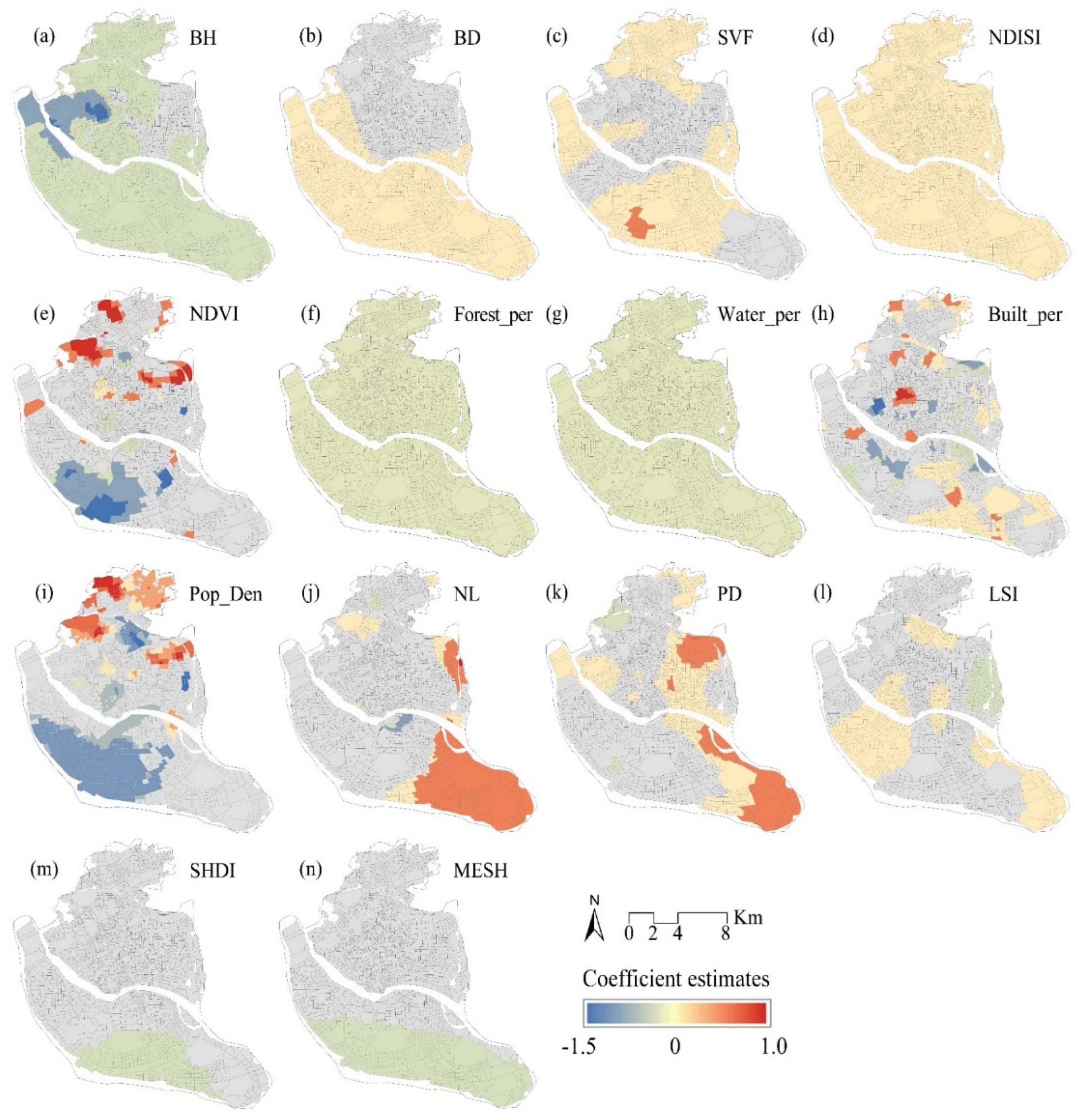
3.4. Spatial Pattern Analysis of Regression Coefficients

Figure 4a shows the proportion of positive and negative influence of each factor on LST. BH, Forest_per, Water_per, SHDI and MESH were negatively correlated with LST, while BD SVF and NDISI were positively correlated with LST. NDVI exhibited mainly negative effects on LST (88.08%), while the opposite occurred for built_per, which had higher proportions of positive than negative effects, with a positive value of 68.56%. The coefficients of both indicators contained both positive and negative values with strong spatial non-stationary, and NL, PD, and LSI had positive effects on LST overall, the negative values accounting for a smaller proportion: 8.91%, 2.32%, and 14.51%, respectively. Pop_Den had almost equal positive and negative proportions, with positive effects accounting for 51.25% and negative effects accounting for 48.75%. Figure 4b shows the statistical distribution of the coefficient estimates for the different variables. In the positive effect, SVF had a greater degree of influence on LST, and BH was an important indicator that affected the reduction of LST. Built_per and pop_den had a wide range of positive and negative coefficients, and the spatial non-smoothness feature was obvious.

Figure 5 shows the spatial distributions of the influencing factor coefficients in the MGWR model. Colored areas represent units with significant local parameter estimates, with positive estimates in red and negative estimates in blue. Estimates in grey units were not significantly correlated. Specifically, among the urban spatial form indicators, BH had the most significant cooling effect in the western part of the urban area, with little change in the northern part of the south, and an overall cooling effect on LST (Figure 5a). The areas with significant correlation between BD and LST were mainly distributed in the south (Figure 5b). The influence range of SVF was basically around the urban area, and the correlation was not significant in the central part of the urban area (Figure 5c).

Among the biophysical parameters, NDVI showed strong spatial non-stationarity characteristics and was spatially distributed mainly in the south and north, with a small aggregation in the central part; some areas in the north had a positive influence on LST (Figure 5e), but the indicator coefficient was negative overall and had a cooling effect on LST. NDISI, on the other hand, is a global variable and had a positive influence on LST in the whole urban area (Figure 5d).

The coefficients for the forest_per and water_per shares of the land-use type factors were small and did not vary significantly spatially, which is consistent with the bandwidth results (Figure 5f,g). However, the overall indicator had a negative effect on LST, indicating that increasing the vegetation and water system shares per unit area have a positive effect on cooling. The built-up percentage, on the other hand, had a positive effect on LST in the southern industrial area, the Gulou district of the city center, and the north railway station (Figure 5h).

The socioeconomic factors also exhibited spatial instability, with population density being negatively correlated with LST in the south and positively correlated in the north (Figure 5i). This is consistent with the trend in the population density distribution (higher in the northern part of Fuzhou City than in the south. NL had a lower degree of influence on LST, and its spatial non-stationarity was more obvious, showing a negative correlation in a smaller area in the north of the city and around Minjiang River, while the eastern part of the city had an obvious spatial aggregation with a positive correlation (Figure 5j).

Among the landscape metrics, PD and LSI had positive effects on LST (Figure 5k,l). SHDI and MESH are negative metrics, mainly distributed in the southern part of the urban area (Figure 5m,n), but the metrics had a lower degree of influence on LST (lower coefficient).

4. Discussion

4.1. Spatial LST Differences

LST distributions were aggregated in Fuzhou, with high LST distributed mainly in the southern (large villages and dense, old, short buildings) and eastern (industrial parks) parts of the city, as well as in the Gulou district at the center of the city (tourist attractions and population catchment area). Denser buildings with narrower streets lead to obstructed ventilation and affect air circulation, and large areas of buildings, which absorb a lot of heat, increase the LST. Large industrial areas with high waste emissions and wastewater lead to higher LSTs. Gulou District, which is a famous tourist area in Fuzhou, is at the center of the city with a high flow of people and dense traffic. In addition, to preserve the integrity of monuments, the buildings in this area are denser and have mostly pedestrian streets, which are not conducive to air flow, leading to higher LST in the area.

4.2. Spatial Heterogeneity of Factors Affecting LST

Comparing the OLS, GWR, and MGWR models, the results indicated that, relative to the OLS model, the GWR and MGWR models had better performances, considered spatial scales and spatial heterogeneity, and could identify the local details of the factors that influenced spatial variations in LST. In addition, the MGWR model had more advantages due to its use of variable bandwidths, which can reflect the differentiated scales of each indicator’s impact on LST.

Building height had a cooling effect on LST: taller buildings can shield more solar radiation and have a larger shaded areas, while wider building spacing and better air conductivity can also lead to cooling effects [51,58,59,60]. The degree of influence of BD and LST was positively correlated, which is also consistent with the results of many previous studies [44], with areas of high building density exhibiting diminished ventilation, while high density means more heat storage and less evaporation, resulting in a consistently high LST environment [30,44]. The SVF showed a more consistent spatial pattern across quarters, with indicator coefficients being positively correlated with LST [30]. Regions with higher SVF values were generally surrounded by lower building density and open sites, implying that more solar heat was absorbed, leading to higher LSTs. Low SVF values indicated shading by vegetation and buildings, more building shading in the center of the urban area, and larger shaded areas, which led to low LSTs [30,61].

The overall effect of NDVI on LST was negatively correlated, but positively correlated with LST in some areas of urban centers [56], meaning that this phenomenon may be related to the reduction of vegetation in urban areas due to urbanization, increased vegetation fragmentation, and differences in vegetation type [62,63]. The NDISI was positively correlated with LST [39], and both NDVI and NDISI exhibited higher degrees of influence on LST [52]. Higher NDVI values indicated that the area has high vegetation cover, which indicates high vegetation evapotranspiration. This contributes to reducing LSTs, while LST increases with increases in the impervious surface area. Impervious surfaces represent the expansion of anthropogenic areas instead of natural landscapes (such as vegetation, water bodies, and wetlands); thus, these surfaces have the greatest degree of influence on LST. Urbanization leads to complex urban landscapes where impervious surfaces contribute to LST as the main influencing factor [51,63]. The overall negative correlations between the water and forests and LST indicates that increasing vegetation and water body areas within the unit scale have a positive effect on reducing LSTs [38].

Among the socioeconomic indicators, population density exhibited spatial instabilities. Population density was significantly positively correlated with LST in the north, and negatively correlated in the south, while the night light index was positively correlated with LST in the east and south, and negatively correlated with a few areas in the urban center. Generally, the distributions of urban hotspots and population concentrations coincided; thus, the more densely populated areas have higher LSTs. However, the population concentration areas in Fuzhou are not located in LST hotspots. The LST of the population concentration area was lower than the core area of the city, with high LST in the north, and the area with the highest night light index was located in the eastern part of the city, which led to the difference in its effect on LST, probably because the hotspots in Fuzhou were distributed in multiple areas, which can lead to the inconsistency between the population distribution and high LST [35].

The landscape metrics exhibited spatial non-stationarity; PD and LSI were positively correlated with LST as a whole [51], while SHDI and MESH were negatively correlated, but the latter two indicators influenced LST to a lesser extent. This indicates that the influence of landscape configuration and diversity factors on LST variation was relatively weak due to the influence of multiple factors [52]. The study area is located in the urban core, with fewer large green areas and relatively fragmented green areas, leading to higher LST. However, the impact of the landscape indicator coefficients on LST were relatively low [52,64].

4.3. Suggestions for Managing Sustainable Development

The results of this study provide a reference for urban planners to mitigate UHIs. The results indicated that spatial heterogeneity leads to different factors influencing LST in different areas. Thus, when planning for different areas, specific analyses of high-LST areas can be targeted to determine corresponding planning strategies. For example, in the eastern part of the urban center, where more industrial concentrations are located, optimizing neighborhood space and reducing waste emissions are methods that can improve the LST. In the southern high LST area, more buildings, unreasonable planning, concentrations of low buildings, less green space, and densely spaced buildings affect air flow and the low reflection of buildings while absorbing heat energy, resulting in high LST. In addition, it is difficult to conduct large area greening in the smaller spaces of older neighborhoods. Therefore, vertical greening and vegetation density should be increased [65,66], while reducing the building density and improving air circulation to alleviate the effect of LST to some extent. Meanwhile, the results of this study indicated that increasing water system areas and the proportion of vegetation can effectively reduce LST. Water systems act as important cooling factors, and their effect on mitigating LST can be higher than that of vegetation. Fuzhou water bodies are more developed; thus, strengthening the management and optimization of the water systems can play a more positive role in cooling [10]. For the landscape pattern index, more fragmented green space patches yielded higher LSTs; thus, increasing the areas of continuous green space patches can improve the cooling effect. Simultaneously, in the context of limited land resources, implementing more stringent greening policies for new expansion areas, combined with an optimal park cooling range and scale, can help to mitigate the negative effects of the UHI effect [67].

4.4. Limitations and Future Research

In this study, 15 common environmental influences were selected to explore the impacts of the factors influencing LST. The results indicated that, due to the complex and variable environment in Fuzhou, the ability of the indicators to explain some parts of the study area remains insufficient, and LST can exhibit more obvious differences during different seasons. Therefore, more detailed and comprehensive indicators are required to analyze urban UHIs in the future, including further analyses of UHIs during different seasons using anthropogenic emissions and weather station data, to improve the performance and reliability of the model.

5. Conclusions

This study used the OLS, GWR, and MGWR models to quantify the spatial relationships between LST and its driving factors in Fuzhou, China. The results showed that the land surface temperature in Fuzhou City shows a more obvious spatial aggregation, and the distribution of high LST is mainly concentrated in the southern and eastern regions. GWR had a better model fit than OLS considering spatial heterogeneity, while MGWR considers the different bandwidths scale between different influence indicators and LST, and the fitting effect was better than GWR. Building density, sky view factor, and normalized difference impervious surface index were significantly positively correlated with LST, building height, forest land percentage, and waterbody percentage were negatively correlated with LST. NDVI, built-up percentage, and population density showed spatially non-stationary characteristics. Among the landscape indicators, PD and LSI showed positive effects on LST, while SHDI and MESH showed lower effects and less explanatory power on LST. These findings indicated that when conducting spatial analysis, it is necessary to consider the influence mechanisms of each influencing factors on LST in different areas and consider the synergistic management under different influencing factors, which can take better integrated measures to mitigate the UHI effect in rapidly urbanizing areas, and is important for guiding urban planning.

References

1. Oke, T.R. City size and the urban heat island. Atmos. Environ. 1973, 7, 769–779. [Google Scholar] [CrossRef]
2. Ceplová, N.; Kalusová, V.; Lososová, Z. Effects of settlement size, urban heat island and habitat type on urban plant biodiversity. Landsc. Urban Plan. 2017, 159, 15–22. [Google Scholar] [CrossRef]
3. Guattari, C.; Evangelisti, L.; Balaras, C.A. On the assessment of urban heat island phenomenon and its effects on building energy performance: A case study of Rome (Italy). Energy Build. 2018, 158, 605–615. [Google Scholar] [CrossRef]
4. Sarrat, C.; Lemonsu, A.; Masson, V.; Guédalia, D. Impact of urban heat island on regional atmospheric pollution. Atmos. Environ. 2006, 40, 1743–1758. [Google Scholar] [CrossRef]
5. Grimm, N.B.; Faeth, S.H.; Golubiewski, N.E.; Redman, C.L.; Wu, J.G.; Bai, X.; Briggs, J.M. Global change and the ecology of cities. Science 2008, 319, 756–760. [Google Scholar] [CrossRef] [Green Version]
6. Song, J.; Yu, H.; Lu, Y. Spatial-scale dependent risk factors of heat-related mortality: A multiscale geographically weighted regression analysis. Sustain. Cities Soc. 2021, 74, 103159. [Google Scholar] [CrossRef]
7. Guo, Y.; Li, S.; Liu, D.L.; Chen, D.; Williams, G.; Tong, S. Projecting future temperature-related mortality in three largest Australian cities. Environ. Pollut. 2016, 208, 66–73. [Google Scholar] [CrossRef] [PubMed]
8. Gasparrini, A.; Guo, Y.; Sera, F.; Cabrera, A.M.V.; Huber, V.; Tong, S.; Coelho, M.D.S.Z.S.; Saldiva, P.H.N.; Lavigne, E.; Correa, P.M.; et al. Projections of temperature-related excess mortality under climate change scenarios. Lancet Planet. Health 2017, 1, e360–e367. [Google Scholar] [CrossRef]
9. Voogt, J.A.; Oke, T.R. Thermal remote sensing of urban climates. Remote Sens. Environ. 2003, 86, 370–384. [Google Scholar] [CrossRef]
10. Du, J.; Xiang, X.; Zhao, B.; Zhou, H. Impact of urban expansion on land surface temperature in Fuzhou, China using Landsat imagery. Sustain. Cities Soc. 2020, 61, 102346. [Google Scholar] [CrossRef]
11. Jiang, Y.; Fu, P.; Weng, Q. Assessing the Impacts of Urbanization-Associated Land Use/Cover Change on Land Surface Temperature and Surface Moisture: A Case Study in the Midwestern United States. Remote Sens. 2015, 7, 4880–4898. [Google Scholar] [CrossRef] [Green Version]
12. Guo, G.; Wu, Z.; Xiao, R.; Chen, Y.; Liu, X.; Zhang, X. Impacts of urban biophysical composition on land surface temperature in urban heat island clusters. Landsc. Urban Plan. 2015, 135, 1–10. [Google Scholar] [CrossRef]
13. Firozjaei, M.K.; Fathololoumi, S.; Kiavarz, M.; Arsanjani, J.J.; Alavipanah, S.K. Modelling surface heat island intensity according to differences of biophysical characteristics: A case study of Amol city, Iran. Ecol. Indic. 2020, 109, 105816. [Google Scholar] [CrossRef]
14. Deng, C.; Wu, C. Examining the impacts of urban biophysical compositions on surface urban heat island: A spectral unmixing and thermal mixing approach. Remote Sens. Environ. 2013, 131, 262–274. [Google Scholar] [CrossRef]
15. Xiao, R.-B.; Ouyang, Z.-Y.; Zheng, H.; Li, W.-F.; Schienke, E.W.; Wang, X.-K. Spatial pattern of impervious surfaces and their impacts on land surface temperature in Beijing, China. J. Environ. Sci. 2007, 19, 250–256. [Google Scholar] [CrossRef]
16. Yu, X.J.; Ng, C.N. Spatial and temporal dynamics of urban sprawl along two urban–rural transects: A case study of Guangzhou, China. Landsc. Urban Plan. 2007, 79, 96–109. [Google Scholar] [CrossRef]
17. Chen, A.; Yao, L.; Sun, R.; Chen, L. How many metrics are required to identify the effects of the landscape pattern on land surface temperature? Ecol. Indic. 2014, 45, 424–433. [Google Scholar] [CrossRef]
18. Zhou, W.; Huang, G.; Cadenasso, M.L. Does spatial configuration matter? Understanding the effects of land cover pattern on land surface temperature in urban landscapes. Landsc. Urban Plan. 2011, 102, 54–63. [Google Scholar] [CrossRef]
19. Estoque, R.C.; Murayama, Y.; Myint, S.W. Effects of landscape composition and pattern on land surface temperature: An urban heat island study in the megacities of Southeast Asia. Sci. Total Environ. 2017, 577, 349–359. [Google Scholar] [CrossRef]
20. Li, W.; Cao, Q.; Lang, K.; Wu, J. Linking potential heat source and sink to urban heat island: Heterogeneous effects of landscape pattern on land surface temperature. Sci. Total Environ. 2017, 586, 457–465. [Google Scholar] [CrossRef]
21. Yao, L.; Li, T.; Xu, M.; Xu, Y. How the landscape features of urban green space impact seasonal land surface temperatures at a city-block-scale: An urban heat island study in Beijing, China. Urban For. Urban Green. 2020, 52, 126704. [Google Scholar] [CrossRef]
22. Du, S.; Xiong, Z.; Wang, Y.-C.; Guo, L. Quantifying the multilevel effects of landscape composition and configuration on land surface temperature. Remote Sens. Environ. 2016, 178, 84–92. [Google Scholar] [CrossRef]
23. Du, H.; Wang, D.; Wang, Y.; Zhao, X.; Qin, F.; Jiang, H.; Cai, Y. Influences of land cover types, meteorological conditions, anthropogenic heat and urban area on surface urban heat island in the Yangtze River Delta Urban Agglomeration. Sci. Total Environ. 2016, 571, 461–470. [Google Scholar] [CrossRef] [PubMed]
24. Huang, G.; Zhou, W.; Cadenasso, M. Is everyone hot in the city? Spatial pattern of land surface temperatures, land cover and neighborhood socioeconomic characteristics in Baltimore, MD. J. Environ. Manag. 2011, 92, 1753–1759. [Google Scholar] [CrossRef]
25. Li, J.; Wang, F.; Fu, Y.; Guo, B.; Yu, H. A Novel SUHI Referenced Estimation Method in Multi-centers Urban Agglomeration with DMSP/OLS Nighttime Light Data. IEEE J. Stars 2020, 13, 1416–1425. [Google Scholar]
26. Liang, Z.; Huang, J.; Wang, Y.; Wei, F.; Wu, S.; Jiang, H.; Zhang, X.; Li, S. The mediating effect of air pollution in the impacts of urban form on nighttime urban heat island intensity. Sustain. Cities Soc. 2021, 74, 102985. [Google Scholar] [CrossRef]
27. Zhang, X.; Estoque, R.C.; Murayama, Y. An urban heat island study in Nanchang City, China based on land surface temper-ature and social-ecological variables. Sustain. Cities Soc. 2017, 32, 557–568. [Google Scholar] [CrossRef]
28. Huang, X.; Schneider, A.; Friedl, M.A. Mapping sub-pixel urban expansion in China using MODIS and DMSP/OLS nighttime lights. Remote Sens. Environ. 2016, 175, 92–108. [Google Scholar] [CrossRef]
29. Dutta, D.; Rahman, A.; Paul, S.; Kundu, A. Impervious surface growth and its inter-relationship with vegetation cover and land surface temperature in peri-urban areas of Delhi. Urban Clim. 2021, 37, 100799. [Google Scholar] [CrossRef]
30. Yin, C.; Yuan, M.; Lu, Y.; Huang, Y.; Liu, Y. Effects of urban form on the urban heat island effect based on spatial regression model. Sci. Total Environ. 2018, 634, 696–704. [Google Scholar] [CrossRef]
31. Oke, T.R. Canyon geometry and the nocturnal urban heat island: Comparison of scale model and field observations. J. Clim. 1981, 1, 237–254. [Google Scholar] [CrossRef]
32. Oke, T.R. Street design and urban canopy layer climate. Energy Build. 1988, 11, 103–113. [Google Scholar] [CrossRef]
33. Unger, J. Connection between urban heat island and sky view factor approximated by a software tool on a 3D urban database. Int. J. Environ. Pollut. 2009, 36, 59. [Google Scholar] [CrossRef] [Green Version]
34. Giridharan, R.; Ganesan, S.; Lau, S. Daytime urban heat island effect in high-rise and high-density residential developments in Hong Kong. Energy Build. 2004, 36, 525–534. [Google Scholar] [CrossRef]
35. Yu, X.; Liu, Y.; Zhang, Z.; Xiao, R. Influences of buildings on urban heat island based on 3D landscape metrics: An investigation of China’s 30 megacities at micro grid-cell scale and macro city scale. Landsc. Ecol. 2021, 36, 2743–2762. [Google Scholar] [CrossRef]
36. Deilami, K.; Kamruzzaman, M.; Liu, Y. Urban heat island effect: A systematic review of spatio-temporal factors, data, methods, and mitigation measures. Int. J. Appl. Earth Obs. Geoinf. 2018, 67, 30–42. [Google Scholar] [CrossRef]
37. Li, S.; Zhao, Z.; Miaomiao, X.; Wang, Y. Investigating spatial non-stationary and scale-dependent relationships between urban surface temperature and environmental factors using geographically weighted regression. Environ. Model. Softw. 2010, 25, 1789–1800. [Google Scholar] [CrossRef]
38. Gao, Y.; Zhao, J.; Han, L. Exploring the spatial heterogeneity of urban heat island effect and its relationship to block morphology with the geographically weighted regression model. Sustain. Cities Soc. 2021, 76, 103431. [Google Scholar] [CrossRef]
39. Chen, X.-L.; Zhao, H.-M.; Li, P.-X.; Yin, Z.-Y. Remote sensing image-based analysis of the relationship between urban heat island and land use/cover changes. Remote Sens. Environ. 2006, 104, 133–146. [Google Scholar] [CrossRef]
40. Zhao, X.; Zhao, Y.; Kuang, D. Seasonal dynamics of the relationship between landscape pattern and land surface temperature in a coastal city. In Proceedings of the 2014 Third International Workshop on Earth Observation and Remote Sensing Applications, Changsha, China, 11–14 June 2014; pp. 418–422. [Google Scholar] [CrossRef]
41. Lu, Y.; Yue, W.; Liu, Y.; Huang, Y. Investigating the spatiotemporal non-stationary relationships between urban spatial form and land surface temperature: A case study of Wuhan, China. Sustain. Cities Soc. 2021, 72, 103070. [Google Scholar] [CrossRef]
42. Cai, Y.; Chen, Y.; Tong, C. Spatiotemporal evolution of urban green space and its impact on the urban thermal environment based on remote sensing data: A case study of Fuzhou City, China. Urban For. Urban Green. 2019, 41, 333–343. [Google Scholar] [CrossRef]
43. Yang, C.; Yan, F.; Zhang, S. Comparison of land surface and air temperatures for quantifying summer and winter urban heat island in a snow climate city. J. Environ. Manag. 2020, 265, 110563. [Google Scholar] [CrossRef] [PubMed]
44. Li, H.; Li, Y.; Wang, T.; Wang, Z.; Gao, M.; Shen, H. Quantifying 3D building form effects on urban land surface temperature and modeling seasonal correlation patterns. Build. Environ. 2021, 204, 108132. [Google Scholar] [CrossRef]
45. Tatem, A.J. WorldPop, open data for spatial demography. Sci. Data 2017, 4, 170004. [Google Scholar] [CrossRef]
46. Zhang, Q.; Seto, K.C. Mapping urbanization dynamics at regional and global scales using multi-temporal DMSP/OLS nighttime light data. Remote Sens. Environ. 2011, 115, 2320–2329. [Google Scholar] [CrossRef]
47. Xu, H. A New Remote Sensing Index for Fastly Extracting Impervious Surface Information. Geomat. Inf. Sci. Wuhan Univ. 2008, 33, 1150–1153. [Google Scholar]
48. Xu, H. Modification of normalised difference water index (NDWI) to enhance open water features in remotely sensed imagery. Int. J. Remote Sens. 2006, 27, 3025–3033. [Google Scholar] [CrossRef]
49. Connors, J.P.; Galletti, C.S.; Chow, W. Landscape configuration and urban heat island effects: Assessing the relationship be-tween landscape characteristics and land surface temperature in Phoenix, Arizona. Landsc. Ecol. 2013, 28, 271–283. [Google Scholar] [CrossRef]
50. Mcgarigal, K.S.; Cushman, S.A.; Neel, M.C.; Ene, E. FRAGSTATS: Spatial Pattern Analysis Program for Categorical Maps. 2002. Available online: www.umass.edu/landeco/research/fragstats/fragstats.html (accessed on 15 September 2020).
51. Li, J.; Song, C.; Cao, L.; Zhu, F.; Meng, X.; Wu, J. Impacts of landscape structure on surface urban heat islands: A case study of Shanghai, China. Remote Sens. Environ. 2011, 115, 3249–3263. [Google Scholar] [CrossRef]
52. Peng, J.; Jia, J.; Liu, Y.; Li, H.; Wu, J. Seasonal contrast of the dominant factors for spatial distribution of land surface temper-ature in urban areas. Remote Sens. Environ. 2018, 215, 255–267. [Google Scholar] [CrossRef]
53. Jiang, W.; Wang, Y.; Dou, M.; Liu, S.; Liu, H. Solving Competitive Location Problems with Social Media Data Based on Cus-tomers’ Local Sensitivities. Int. J. Geoinf. 2019, 8, 202. [Google Scholar]
54. Oshan, T.M.; Li, Z.; Kang, W.; Wolf, L.J.; Fotheringham, A.S. mgwr: A Python Implementation of Multiscale Geographically Weighted Regression for Investigating Process Spatial Heterogeneity and Scale. ISPRS Int. J. Geoinf. 2019, 8, 269. [Google Scholar] [CrossRef] [Green Version]
55. Zhao, C.; Jennifer, J.; Weng, Q.; Russell, W. A Geographically Weighted Regression Analysis of the Underlying Factors Related to the Surface Urban Heat Island Phenomenon. Remote Sens. 2018, 10, 1428. [Google Scholar] [CrossRef] [Green Version]
56. Guo, A.; Yang, J.; Sun, W.; Xiao, X.; Cecilia, J.X.; Jin, C.; Li, X. Impact of urban morphology and landscape characteristics on spatiotemporal heterogeneity of land surface temperature. Sustain. Cities Soc. 2020, 63, 102443. [Google Scholar] [CrossRef]
57. Burnham, K.; Anderson, D. Multimodel inference: Understanding AIC and BIC in Model Selection. Sociol. Methods Res. 2004, 33, 261–304. [Google Scholar] [CrossRef]
58. Zhang, N.; Zhang, J.; Chen, W.; Su, J. Block-based variations in the impact of characteristics of urban functional zones on the urban heat island effect: A case study of Beijing. Sustain. Cities Soc. 2021, 76, 103529. [Google Scholar] [CrossRef]
59. Perini, K.; Magliocco, A. Effects of vegetation, urban density, building height, and atmospheric conditions on local temperatures and thermal comfort. Urban For. Urban Green. 2014, 13, 495–506. [Google Scholar] [CrossRef]
60. Alavipanah, S.; Schreyer, J.; Haase, D.; Lakes, T.; Qureshi, S. The effect of multi-dimensional indicators on urban thermal conditions. J. Clean. Prod. 2017, 177, 115–123. [Google Scholar] [CrossRef]
61. Yang, X.; Li, Y. The impact of building density and building height heterogeneity on average urban albedo and street surface temperature. Build. Environ. 2015, 90, 146–156. [Google Scholar] [CrossRef]
62. Chun, B.; Guldmann, J.M. Impact of greening on the urban heat island: Seasonal variations and mitigation strategies. Comput. Environ. Urban Syst. 2018, 71, 165–176. [Google Scholar] [CrossRef]
63. Masoudi, M.; Tan, P.Y.; Fadaei, M. The effects of land use on spatial pattern of urban green spaces and their cooling ability. Urban Clim. 2020, 35, 100743. [Google Scholar] [CrossRef]
64. Xiang, Y.; Huang, C.; Huang, X.; Zhou, Z.; Wang, X. Seasonal variations of the dominant factors for spatial heterogeneity and time inconsistency of land surface temperature in an urban agglomeration of central China. Sustain. Cities Soc. 2021, 75, 103285. [Google Scholar] [CrossRef]
65. Azhdari, A.; Soltani, A.; Alidadi, M. Urban morphology and landscape structure effect on land surface temperature: Evidence from Shiraz, a semi-arid city. Sustain. Cities Soc. 2018, 41, 853–864. [Google Scholar] [CrossRef]
66. Chen, M.; Dai, F.; Yang, B.; Zhu, S. Effects of neighborhood green space on PM2.5 mitigation: Evidence from five megacities in China. Build. Environ. 2019, 156, 33–45. [Google Scholar] [CrossRef]
67. Yao, X.; Yu, K.; Zeng, X.; Lin, Y.; Ye, B.; Shen, X.; Liu, J. How can urban parks be planned to mitigate urban heat island effect in “Furnace cities”? An accumulation perspective. J. Clean. Prod. 2021, 330, 129852. [Google Scholar] [CrossRef]
Figure 1. Study area: (a) Fujian Province, China; (b) Fuzhou City, Fujian Province; (c) land cover map of the study area based on satellite imagery from GF-1 (2018).
Remotesensing 14 01266 g001
Figure 2. (a) Spatial distribution of land surface temperature (LST); (b) local indicators of spatial associations (LISA); (c) Global Moran’s I of LST.
Remotesensing 14 01266 g002
Figure 3. (a) Local R2 values for the GWR and (b) MGWR models.
Remotesensing 14 01266 g003
Figure 4. (a) Proportions of positive and negative effects of the different variables; (b) box plots of coefficients for the different variables.
Remotesensing 14 01266 g004
Figure 5. (an) Spatial distribution of the coefficients of each variable. Red indicates a positive correlation with LST, blue indicates a negative correlation, and gray indicates no spatial correlation.
Remotesensing 14 01266 g005