From Regression Based on Dynamic Filter Network to Pansharpening by Pixel-Dependent Spatial-Detail Injection

Abstract

Compared with hardware upgrading, pansharpening is a low-cost way to acquire high-quality images, which usually combines multispectral images (MS) in low spatial resolution with panchromatic images (PAN) in high spatial resolution. This paper proposes a pixel-dependent spatial-detail injection network (PDSDNet). Based on a dynamic filter network, PDSDNet constructs nonlinear mapping of the simulated panchromatic band from low-resolution multispectral bands through filtering convolution regression. PDSDNet reduces the possibility of spectral distortion and enriches spatial details by improving the similarity between the simulated panchromatic band and the real panchromatic band. Moreover, PDSDNet assumes that if an ideal multispectral image that has the same resolution with the panchromatic image exists, each band of it should have the same spatial details as in the panchromatic image. Thus, the details we fill into each multispectral band are the same and they can be extracted effectively in one pass. Experimental results demonstrate that PDSDNet can generate high-quality fusion images with multispectral images and panchromatic images. Compared with BDSD, MTF-GLP-HPM-PP, and PanNet, which are widely applied on IKONOS, QuickBird, and WorldView-3 datasets, pansharpened images of the proposed method have rich spatial details and present superior visual effects without noticeable spectral and spatial distortion.

1. Introduction

Remote sensing sensors generate images by capturing information of electromagnetic waves reflected off the Earth’s surface. However, it is arduous to obtain images with both high spatial resolution and high spectral resolution simultaneously. The energy received by the sensor is double the integral of the electromagnetic wave in space and wavelength. Generating images with higher spatial and spectral resolution means that the energy is integrated at shorter wavelengths and in smaller areas. Consequently, the energy is weaker, resulting in poorer image qualities. Only one can be enhanced at a time. Thus, it is challenging to acquire high-quality images with high spectral and spatial resolution, limited by the equipment on remote sensing platforms. Compared with hardware upgrading, pansharpening is a low-cost way to sufficiently utilize data to obtain high spectral and spatial resolution images. Pansharpening combines multispectral images (MS) with low spatial resolution and panchromatic images (PAN) with high spatial resolution.

A promising pansharpening method should produce results that meet following requirements:

• Spectral fidelity: The spatial information of fusion result should be as close as possible to the spatial information of original MS. Chromatic aberration and spectral distortion should be avoided.
• Exact spatial details: The spatial details of fusion result should be as close as possible to details of original PAN. Blur, lack, and distortion of details should be avoided.

Up to now, pansharpening methods fall into three main categories: the first one is component substitution (CS), the second one is multi-resolution analysis (MRA), and the third one is deep learning (DL). A quick review of these three main methods is described as follows.

• The CS-based method is a class of methods that decompose MS into spectral information and structural information, then substitute the structural information with PAN, such as intensity–hue–saturation transform (IHS) [1,2,3,4], brovey transform (BT) [5], Gram–Schmidt transform (GS) [6,7], principal component analysis (PCA) [8,9], band-dependent spatial-detail (BDSD) [10], partial replacement adaptive component substitution (PRACS) [11], etc. Higher correlation between the PAN and the component being replaced will reduce the distortion of the fused image.
• The MRA-based method is a class of methods that adopt a multi-resolution decomposition on the PAN for low-frequency information, and then inject the details from the differences between them into MS. The way of decomposition can be based on wavelets [12], for instance, undecimated wavelet transform (UDWT) [13], decimated wavelet transform (DWT) [14,15], “à trous” wavelet transform (ATWT) [16,17,18], or not, such as Laplacian pyramid (LP) [19]. The key is to find a filter to acquire the low frequency component and the most common being the modulation transfer function (MTF) [20,21,22].
• The deep-learning-based method [23] is a rapidly developing pansharpening method in recent years. Deep-learning-based methods commonly develop on the structure of super-resolution methods [24], such as PNN [25], DRPNN [26], and MSDCNN [27]. Some methods combine component substitution and nonlinear mapping, for example, PanNet [28], Target-PNN [29], cross-scale learning model based on Target-PNN [30], RSIFNN [31], etc. These methods do not just regard the output of deep convolution network as fusion result, but apply the deep network to learn the details MS lacked, then attach the details to the upsampled MS to generate fusion image. In addition, deep-learning-based methods have another branch based on generative adversarial network (GAN) [32] that combines the theory of reinforcement learning (RL), for instance, PSGAN [33], RED-cGAN [34], Pan-GAN [35], PanColorGAN [36], etc. With a two-stream structure model, PSGAN [33] based on TFNet [37] accomplishes fusion in feature domain. PanColorGAN [36] based on CS, regarding pansharpening as a guided colorization task rather than a super-resolution task.

From the process of fulfilling pansharpening, the CS-based and MRA-based methods are dedicated to solving the following sub-problems, i.e., details extraction and details injection.

Regardless of details injection, as far as details extraction is concerned, both CS-based and MRA-based methods assume that the details come from the differences between the high spatial resolution PAN and the low spatial resolution PAN. The difference lies only in how the low spatial resolution PAN is acquired. In most CS-based methods, the low spatial resolution PAN is assumed to be a linear combination of low spatial resolution multispectral bands. In contrast, in MRA-based methods, the low spatial resolution PAN is assumed to be the low-frequency version of the high spatial resolution PAN.

The DL-based methods directly construct a convolution neural network (CNN) model to represent the relationship between lower spatial resolution multispectral bands and higher spatial resolution PAN by training down-sampled data, then directly apply the CNN model to the higher spatial resolution PAN to obtain sharpened multispectral bands. The relationship constructed by the CNN model is non-linear.

In this article, we propose a novel CS-based pansharpening method that employs an adaptive filter model as the non-linear combination mapping between the low spatial resolution PAN and the low spatial resolution multispectral bands. Further, we extract the details in the same way as CS-based method by the difference between the high spatial resolution PAN and the low spatial resolution PAN, then inject details back to the low spatial resolution multispectral bands. The adaptive filter model is a pixel-dependent spatial-detail injection model. Our method combines multispectral bands to obtain a low-resolution PAN through pixel-dependent local band adaptive filter convolution. The adaptive filters of multispectral bands are generated based on a “dynamic filter network” (DFN) [38]. The DFN adopts an encoder–decoder structure to learn the location-dependent kernel and applies a separate subnet to predict the convolution filter weight at each pixel. The network learns in a supervised way and has high flexibility due to its self-adaptability.

The proposed method presents superior visual effects due to the following aspects:

(1)

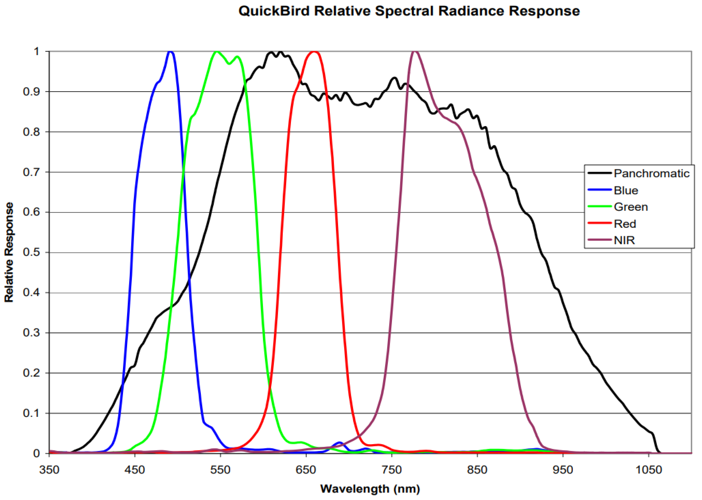
Based on the dynamic filter network, the nonlinear mapping between the panchromatic band and the low-resolution multispectral bands through filter convolution regression is constructed. Compared with other CS-based methods, the proposed method is more reasonable. Figure 1 shows spectral response functions of panchromatic and multispectral imagery for QuickBird sensors. Spectral response functions are similar to a normal distribution of a single peak function. Obviously, it is challenging to generalize the radiance between PAN and multispectral bands by linear combination model. Traditional CS-based methods are not completely accurate.

(2)

Assuming that if an ideal MS that has the same resolution with PAN exists, each band of it should have the same spatial details as in PAN, spatial details are acquired in the same way as CS-based method from the differences between the high spatial resolution PAN and the low spatial resolution PAN, then inject the details back to the low spatial resolution multispectral bands; therefore, the pansharpened images have rich spatial details. Compared with PNN-based methods, the proposed method is more explainable.

(3)

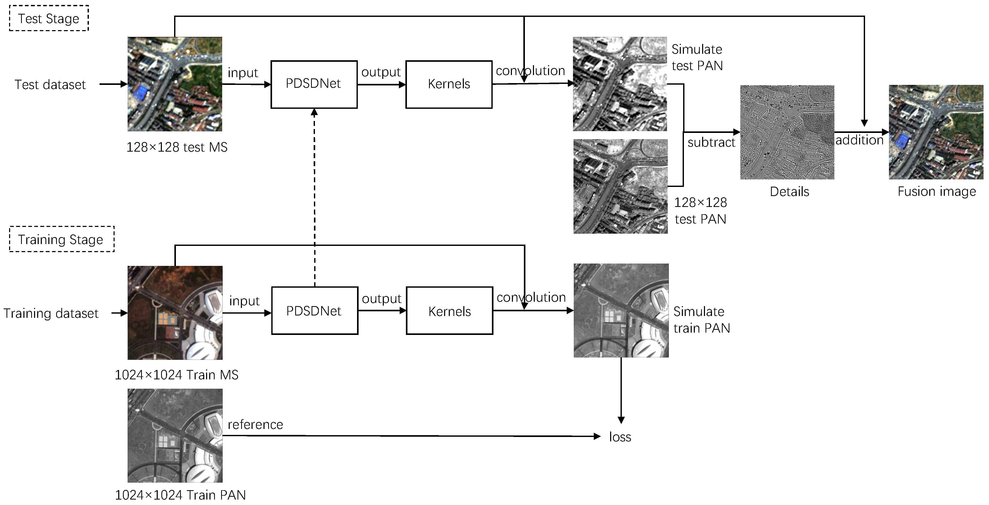
Different from the general DL-based fusion method, no extra work is required to make truth values at a small scale. In most image fusion methods, training datasets and ground truth need to be made artificially at the downscale level to learn the mapping between MS, PAN, and fusion images in reduced resolution then apply it on a larger scale.

We have introduced an overview of traditional fusion methods and methods based on deep learning. The rest of this paper is organized as follows: In Section 2, firstly, we focus on the development of the injection model and propose the pixel-dependent spatial-detail injection model (PDSDNet), then we introduce DFN and describe the adaptations that were made for the application of DFN to remote sensing. Next, we describe datasets and the process of our experiments in detail, and the results are shown in Section 3. The last Section 4 draws our conclusion.

2. Pixel-Dependent Spatial-Detail Network and Dynamic Filter Network

Let $MS$ represent original multispectral image (MS) and $M{S}_b$ denote the b-th band of $MS$. B is the total number of MS bands, and b is from 1 to B. For example, $M{S}_1$ represents the first band of original MS. $\widetilde{M{S}_b}$ is the upsampled $M{S}_b$. P is the original panchromatic image (PAN) and $P_{LP}$ is the low-resolution PAN. The size of $\widetilde{M{S}_b}$ is the same as original PAN. F is the fused image, $F_b$ represents the b-th band of the fused image. $L_1$ and $L_2$ is the width and height of the image of PAN. The resolution ratio of PAN and MS is R. For IKONOS, QuickBird, and WorldView-3 images, the value of the scale ratio R is four.

For CS-based spatial-detail model, we recall that Andrea Garzelli presented two linear injection models [10]. The first model is the single spatial-detail (SSD) image model, and the model extracts a spatial-detail image from the PAN band by subtracting low-pass version PAN, which can be obtained with convolution by an MTF-shaped filter with approximately 1/R cutoff frequency [20]. Alternatively, the low-pass version can be obtained by the linear regression of overlapped multispectral bands; the second model is the band-dependent spatial-detail (BDSD) model, which adopts different detail images extracted from the PAN band to pansharpen MS depending on the particular MS band.

We present the third model, a pixel-dependent spatial-detail network (PDSDNet) model, which extracts the details from the PAN and low-pass version PAN. The low-resolution PAN is generated by filters particularly depending on the pixel of MS.

2.1. SSD Model & BDSD Model

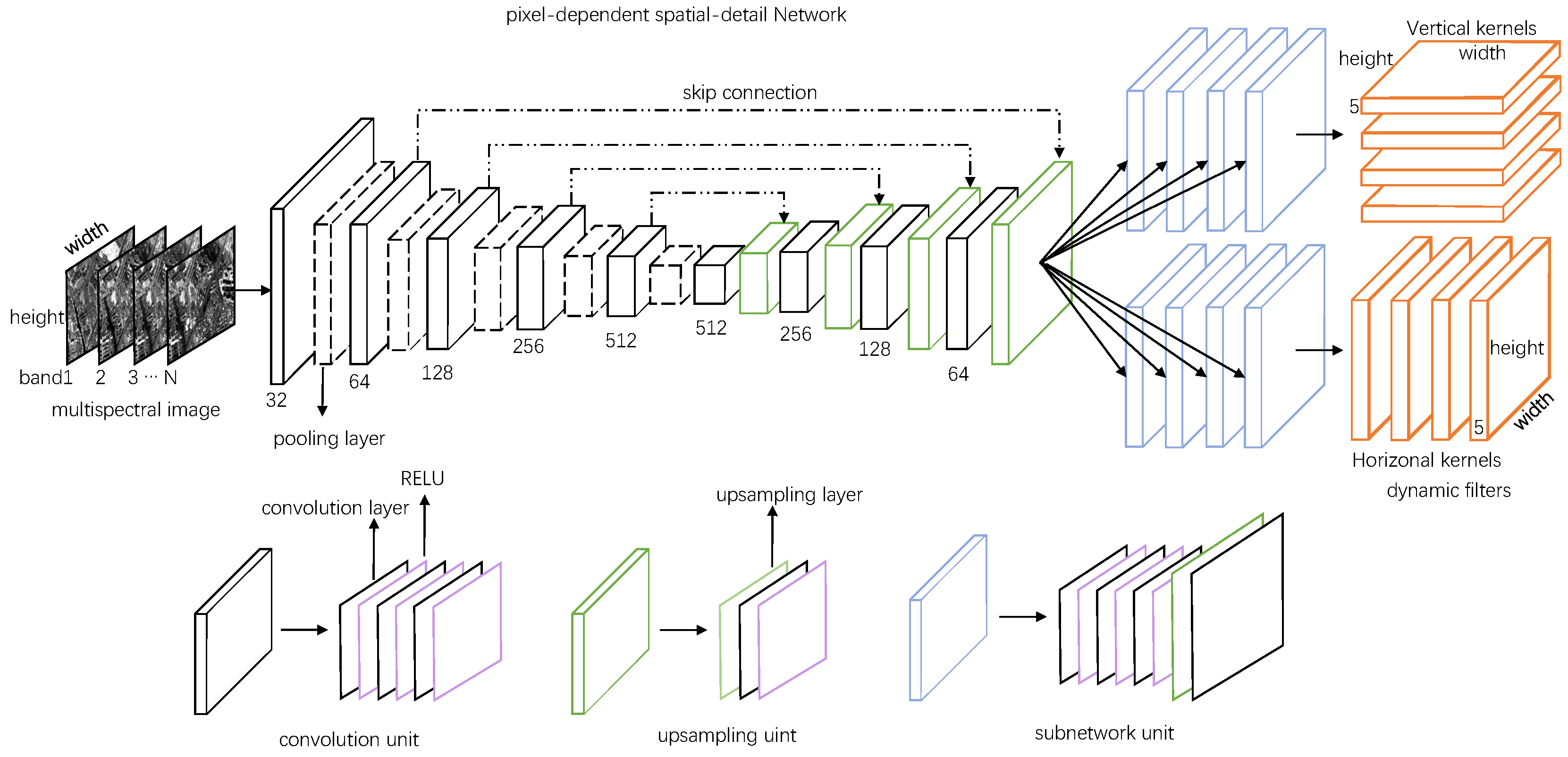
In the SSD model, such as IHS transform as the representative of component substitution, the low-resolution panchromatic image is substantially regarded as a linear combination of multiple bands from the multispectral image. Thus, approximate PAN with weighted parameters is described as Equation (1).

$$F_b={\widetilde{MS}}_b+g_b(P-P_{LP})$$

(1)

where $g_b$ is a gain parameter of the b-th band that controls the injection of the extracted details. $P_{LP}$ is the simulated panchromatic image, $P-P_{LP}$ is the spatial details MS lacked. $\widetilde{M{S}_b}$ is the b-th band of the upsampled version of the low spatial resolution MS. In the component substitution method, $P_{LP}$ is the intensity component of MS which is the weighted combination of MS bands, as Equation (2). In the SSD model, the detail image is the same for all MS bands.

$$P_{LP}=\sum _{b=1}^B{w}_b{\widetilde{MS}}_b$$

(2)

$w_b$ is the weighting coefficient of the b-th MS band, B is the number of bands. Many CS-based pansharpening algorithms rely upon Equation (1), just changing the ways to estimate the injection coefficient $g_b$ and the weight $w_b$. In IHS transform, $w_b=1/B$.

In the BDSD model, Equation (1) could be further rewritten in the following Equation (3):

$$F_b={\widetilde{MS}}_b+g_b(P-\sum _{k=1}^B{w}_{b,k}{\widetilde{MS}}_b)$$

(3)

here detail image extracted from PAN is calculated for each MS band by evaluating a band-dependent generalized intensity from the B MS bands.

2.2. PDSDNet Model

We propose a non-linear spatial-detail model in which the detail image is extracted for each pixel from PAN. The detail image is calculated by evaluating a pixel-dependent generalized intensity from the B MS bands, as Equation (4). Only the MS bands overlapped with the PAN band participate in calculating.

$$P_{LP,(x,y)}=\sum _{b=1}^B{\widetilde{MS}}_{b,(x,y)}\ast D{F}_{b,(x,y)}$$

(4)

where $(x,y)$ denotes the position of the pixel in image, ∗ means the convolution operator, $D{F}_{b,(x,y)}$ denotes the adaptive convolution kernel or filter depending on MS band b and pixel position, which is obtained by a dynamic filter network (DFN). For each band, convolution will be achieved through a sliding window whose size is the same as the convolution kernel.

According to the model of CS-based methods, the pansharpened image $F_b$ is equal to the sum of the upsampled MS band ${\widetilde{MS}}_b$ and the injected details $P-P_{LP,(x,y)}$. Here we ignore the injection coefficients considering that the detail image is pixel-dependent spatial-detail by adaptive filter network; therefore, the PDSDNet can be summarized as Equation (5):

$$F_b={\widetilde{MS}}_b+(P-P_{LP,(x,y)})$$

(5)

In low-resolution PAN $P_{LP,(x,y)}$, the parameters of adaptive filters $D{F}_{b,(x,y)}$ can be learned from a large-scale training dataset by approximating $P_{LP,(x,y)}$ to P. Accordingly, the loss function of network for simulating PAN is designed to measure the similarity of ground truth P and the result of the network $P_{LP,(x,y)}$. The loss function is described as Equation (6):

$$Loss=\frac{1}{N}\sum _{k=1}^N{∥P_{\left\{k\right\}}-{\{\sum _{b=1}^B{\widetilde{MS}}_{b,(x,y)}\ast D{F}_{b,(x,y)}\}}_{\left\{k\right\}}∥}_F^2$$

(6)

where N represents the number of training examples, ${\parallel ·\parallel }_F$ is the Frobenius norm, and $P_{\left\{k\right\}}$ is the k-th example PAN extracted from the ground truth image.

Minimize $Loss$ to train the network for simulating PAN and the pansharpened image can be calculated by Equation (5).

2.3. Dynamic Filter Network (DFN)

The adaptive filters $\left\{D{F}_{b,(x,y)}\right\}$ are obtained locally and dynamically depending on the input images by the dynamic filter generation network [38]. In DFN, parameters consist of model parameters and dynamically generated parameters. Model parameters, that is the layer parameters, are initialized in advance and only updated during training. When the train is finished, model parameters are fixed and are the same for all test samples. Dynamically generated parameters do not need to be initialized and are sample-specifically generated on the fly. Dynamically generated parameters denote dynamic filters in our method. The filter generating network dynamically outputs generated parameters, while its own parameters are part of the model parameters. Dynamic filters of our method are implemented by generating two convolution kernels per pixel instead of sharing a convolution kernel across the full image, thus enhancing the adaptability of the network.

The filter generation network is shown in Figure 2. The encoder–decoder block is used as the main component, which includes four units: convolution, pooling, upsampling, and subnetwork. The convolution unit is composed of three convolution layers and activation layers alternately. The pooling unit is an average pooling layer. The upsampling unit consists of upsampling layer, convolution layers and activation layer. The way of upsampling is bilinear interpolation. The convolution unit and the upsampling unit constitute the subnetwork unit. The network inputs B bands MS and outputs B groups of filters for simulating PAN. MS is convolved with these filters to obtain the simulated PAN.

For the inspiration of [39,40,41], our adaptive filters $D{F}_{b,(x,y)}$ have two separable single-dimensional convolution kernels for each band b and each pixel: vertical kernel and horizontal kernel. $D{F}_{b,(x,y)}$ is k × k patch in the center of $x,y$ if the size of vertical kernel and horizontal kernel is k.

2.4. Implementation Details

We chose three datasets from different satellites for experiments in

Table 1. Details of datasets.

Satellite	Sensor	Spatial Resolution	Spectral Resolution	Band Number & Band	Size	Data Volume
IKONOS	Pan	1 m	1 band	1 Pan	1024 × 1024	200
	MS	4 m	4 bands	1 Blue, 2 Green, 3 Red, 4 NIR	256 × 256 × 4	200
QuickBird	Pan	0.61 m	1 band	1 Pan	1024 × 1024	500
	MS	2.44 m	4 bands	1 Blue, 2 Green, 3 Red, 4 NIR	256 × 256 × 4	500
WorldView-3	Pan	0.31 m	1 band	1 Pan	1024 × 1024	160
	MS	1.24 m	8 bands	1 Costal, 2 Blue, 3 Green, 4 Yellow, 5 Red, 6 Red Edge, 7 NIR, 8 NIR2	256 × 256 × 4	160

. Before the experiment, the data need to be preprocessed. Firstly, 256 × 256 MS is upsampled to the same 1024 × 1024 size as PAN. Secondly, MS and PAN are normalized with Z-Score normalization (zero-mean normalization), which makes the mean of images become 0 and the standard deviation 1. Thirdly, the data are randomly divided into two parts, 90% for the training stage and 10% for the testing stage. Further, the data for the training stage are cropped into 128 × 128 patches in two ways. One is sequentially cropping in step size 64, and the other is randomly cropping, which randomly selects 100 points on the graph as the center point. So 325 patches in size of 128 × 128 are produced from each 1024 × 1024 image. The result is 20% of patches for validation and 80% for training in the training process.

The process is illustrated as Figure 3. The experiments were implemented by PyTorch, a common deep learning framework. The input of the network is the upsampled and normalized MS, which are four bands, and the output is the simulated PAN, the reference of which is the normalized PAN. We set the batch as 20 and kernel size 5. The convolution kernel of the convolution layer is 3 × 3 with stride 1 and padding 1. The convolution kernel of the average pooling layer is 2 × 2 with stride 2 in the encoding process. Correspondingly, the scale factor of the upsampling layer is 2 in the decoding process. The optimizer is an Adam optimizer with an initial learning rate of 0.001. The loss function is mean-square error (MSE) as Equation (6).

3. Experiments and Results

To assess the performance of the proposed methods, we have implemented multiple experiments with real-world multi-resolution images, exploring a wide range of situations. Consider the typical case when training and test data are acquired with the same sensor but come from different scenes, three state-of-the-art algorithms are employed for comparison, which are BDSD [10], MTF-GLP-HPM-PP [22], and PanNet [28]. BDSD is one of the usual methods of CS [42], which is an accurate linear injection model in the minimum mean-square-error (MMSE) sense. BDSD extracts details by evaluating a band-dependent generalized intensity from the MS bands. CS-based methods are inclined to generate spectral distortion but usually have no obvious spatial distortion. MTF-GLP-HPM-PP is one of the effective methods of MRA [42], which is based on a generalized Laplacian pyramid (GLP) [43] with modulation transfer function (MTF)-matched filter [20], multiplicative injection model [44] and post-processing (MTF-GLP-HPM-PP) [22]. MRA-based methods are prone to spatial distortion but generally have little spectral distortion. PanNet is a fusion method based on deep learning, which trains network parameters in the high-pass filtering domain rather than the image domain. PanNet learns the details from high-frequency information of MS and PAN, then adds upsampled MS to the network output. These methods have a common pre-processing step, applying MTF to process the image. This step is not performed in PDSDNet.

3.1. Datasets for Experiments

The data of our experiments were selected from a special large-scale publicly available benchmark dataset for pansharpening from [42]. HR PAN images are 1024 × 1024 and LR MS images are 256 × 256. In addition, the geometrical registration of datasets has been performed in [42]. These data contain a variety of features such as urban, green vegetation, water scenario, and mixed features. Considering satellites, spatial resolution and number of bands, we chose datasets of three satellites from [42]. The datasets consist of 200 IKONOS, 500 QuickBird, and 160 WorldView-3 image patches in different spatial resolutions. As Table 1 shows, the multispectral image (MS) of IKONOS and QuickBird have four bands while WorldView-3 has eight.

Table 2. Band settings of different satellites.

Satellite	Pan	Coastal	Blue	Green	Yellow	Red	Red Edge	NIR	NIR2
IKONOS	450–900		450–530	520–610		640–720		760–860
QuickBird	450–900		450–520	520–600		630–690		760–900
WorldView-3	450–800	400–450	450–510	510–580	585–625	630–690	705–745	770–895	860–1040

shows the wavelength of bands of different satellite sensors. “Pan” corresponds to the band range of panchromatic image, and from “Coastal” to “NIR2” is the first to eighth band corresponding to the multispectral image of WorldView-3. “Blue”, “Green”, “Red”, and “NIR” are the first to the fourth band of the multispectral image of IKONOS and QuickBird.

The four bands of IKONOS’s MS overlap with PAN, and they were all put into the network for simulating PAN, so is QucikBird. It is important to note that our method utilizes only six bands of WorldView-3 from Blue to NIR for simulating PAN because the range of Coastal and NIR2 have no overlap with PAN; however, in other cases, the data of WorldView-3 is processed with eight bands. Assuming that if an ideal MS that has the same resolution with PAN exists, each band of it should have the same spatial details as in PAN, the details obtained by simulated PAN and original PAN are added to eight bands, not six.

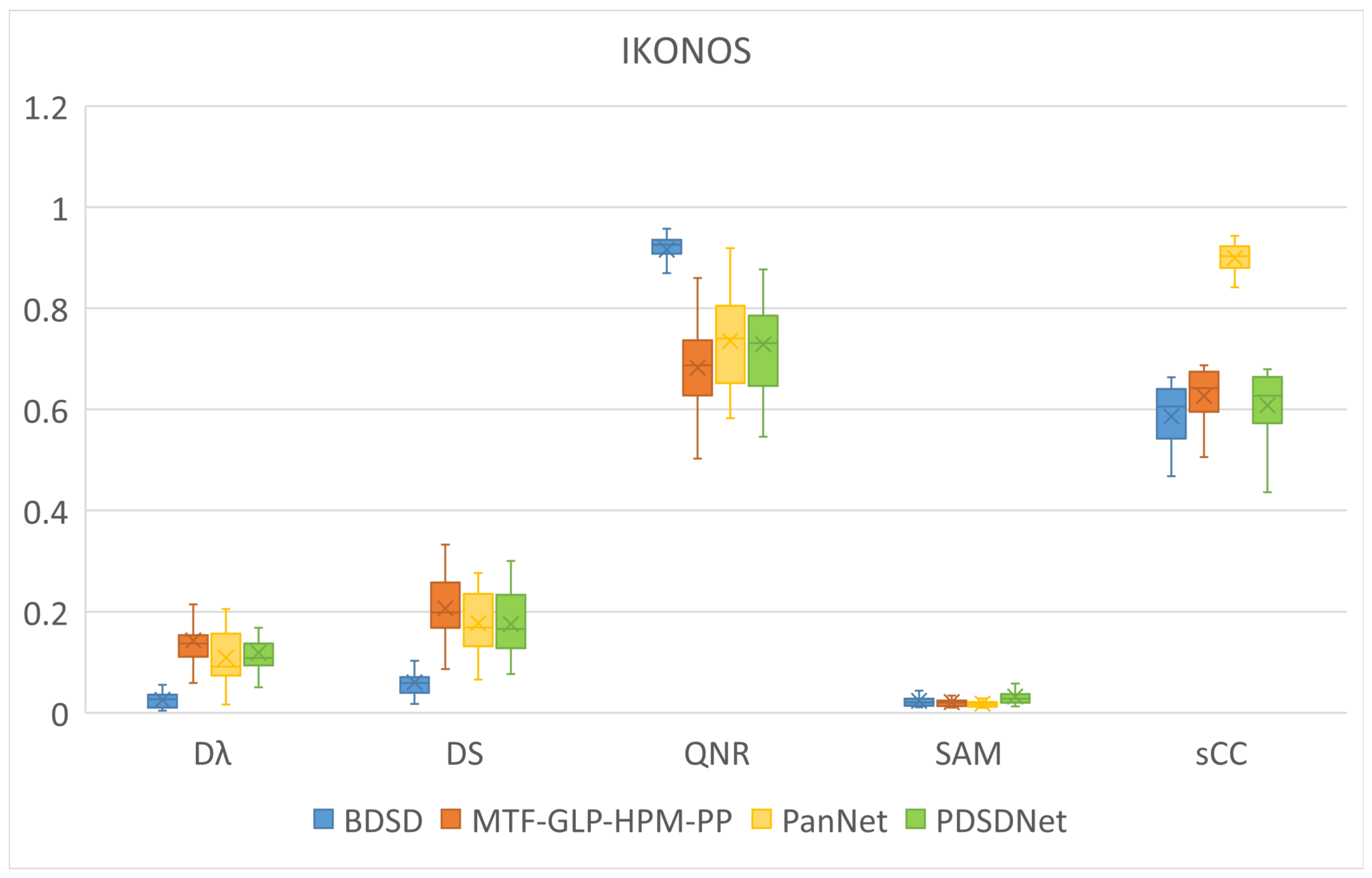
3.2. Evaluation Indexes

In addition to visual evaluation, we have chosen two types of five indexes for quality assessment. One type is full-resolution assessment, which infers the quality of the pansharpened image at the scale of the PAN image without resorting to a single no-reference image [45]. The index of the quality with no reference (QNR) [46], the spectral distortion $D_{\lambda }$ and the spatial distortion $D_S$ are contained in this type. QNR measures spectral and spatial consistencies by calculating mutual similarities between any couples of MS bands and each MS band and PAN. The consistencies are assumed unchanged on average before and after fusion. Another type is reduced-resolution assessment, which measures the similarity of the fused product and an ideal reference, i.e., the original MS. The index of spectra mapper angle (SAM) [47] and spatial correlation coefficient (sCC) [48] are chosen for this purpose.

QNR, SAM, and sCC are calculated as

Table 3. Quality indexes.

Index	Equation	Meaning
$D_{\lambda }$	$D_{\lambda }=\frac{1}{B(B-1)}{\sum }_{b=1}^B{\sum }_{j=1,j\ne b}^B\left|UIQI(F_b,F_j)-UIQI(M{S}_b,M{S}_j)\right|$	the smaller the better
$D_S$	$D_S=\frac{1}{B}{\sum }_{b=1}^B\left|UIQI(F_b,P)-UIQI(M{S}_b,P_{LP})\right|$	the smaller the better
QNR	$QNR=(1-D_{\lambda })(1-D_S)$	the bigger the better
SAM	$SAM=\frac{1}{L_1{L}_2}{\sum }_{i=1}^{L_1{L}_2}arccos\frac{{\sum }_{b=1}^B(R_{i,b}·F_{i,b})}{\sqrt{{\sum }_{b=1}^B{R}_{i,b}^2}\sqrt{{\sum }_{b=1}^B{F}_{i,b}^2}}$	the smaller the better
sCC	$sCC=\frac{{\sum }_{b=1}^B{\sum }_{i=1}^{L_1{L}_2}(\widehat{P_{i,b}}·\widehat{F_{i,b}})}{\sqrt{{\sum }_{b=1}^B{\sum }_{i=1}^{L_1{L}_2}{\widehat{P_{i,b}}}^2}\sqrt{{\sum }_{b=1}^B{\sum }_{i=1}^{L_1{L}_2}{\widehat{F_{i,b}}}^2}}$	the bigger the better

, where symbols used have the same meaning as in Section 2. $MS$ is the multispectral image (MS), P is the panchromatic image (PAN) and $P_{LP}$ is the low-resolution PAN, F is the fused image, R is the reference image. B is the total number of MS bands, $F_{i,b}$ represents the value of position i in b-th band of the fused image, b is an integer from 1 to B. When the correlation coefficient between PAN and fusion image or MS is calculated, PAN with only one band will be replicated B times to obtain B bands for convenience of calculation. $P_{i,b}$ is the same when b takes any integer value between 1 and B. ^denotes the image processed through high-pass filter. $L_1$ and $L_2$ is the width and height of an image. ${\sigma }_I$ represents the standard variance of image vector I and ${\sigma }_{IJ}$ is the covariance of I and J. $\overline{I}$ denotes the mean value of I.

It is noted that QNR is the unique quality index combined two distortions of the spectral distortion $D_{\lambda }$ and the spatial distortion $D_S$ as Equation (7):

$$QNR={(1-D_{\lambda })}^{\alpha }{(1-D_S)}^{\beta }$$

(7)

where usually $\alpha =\beta =1$, and $QNR\in [0,1]$ with 1 being the best attainable value. The spectral distortion $D_{\lambda }$ and the spatial distortion $D_S$ both are calculated through universal image quality index (UIQI) [49] defined as Equation (8):

$$UIQI(I,J)=\frac{{\sigma }_{IJ}}{{\sigma }_I{\sigma }_J}·\frac{2\overline{I}\overline{J}}{{\overline{I}}^2+{\overline{J}}^2}·\frac{2{\sigma }_I{\sigma }_J}{{\sigma }_I^2+{\sigma }_J^2}$$

(8)

Obviously, UIQI is a comprehensive index calculating the similarity between two images, which is a combination of three factors: loss of correlation, luminance distortion, and contrast distortion. If the value of UIQI is 1, it means that the image has the best fidelity for the reference image.

The description of each index in Table 3 is described as follows:

• $D_{\lambda }$ represents the spectral distortion of the image. $D_{\lambda }$ calculates the correlation of the interband between the UIQI of the fused image and the reference image. Smaller $D_{\lambda }$ means smaller spectral distortion of the fused image, and so is SAM. If $D_{\lambda }$ is 0, the fused image has no spectral distortion.
• $D_S$ shows the spatial distortion of the image. $D_S$ measures the correlation of the interband between the UIQI of fused image and PAN. Smaller $D_S$ represents smaller spatial distortion. If $D_S$ is 0, the fusion image has no spatial distortion.
• QNR stands for no reference quality index and measures the quality of full-resolution fused images. QNR is the combination of $D_{\lambda }$ and $D_S$. Bigger QNR denotes better image quality. When both of $D_{\lambda }$ and $D_S$ are 0, QNR will be 1, which means the fusion image has effective quality.
• SAM measures spectral mapper angle between the fused image and the reference image. Smaller spectral distortion corresponds to smaller SAM. It means perfect image when SAM goes to 0. SAM is expressed in radians in our indexes.
• sCC calculates the spatial correlation coefficient between the fusion image and PAN. The spatial details of PAN and fused image are obtained by high-pass filtering, such as Sobel operator measuring horizontal edge. A greater relative relationship leads to bigger sCC. The optimal value of sCC is 1.

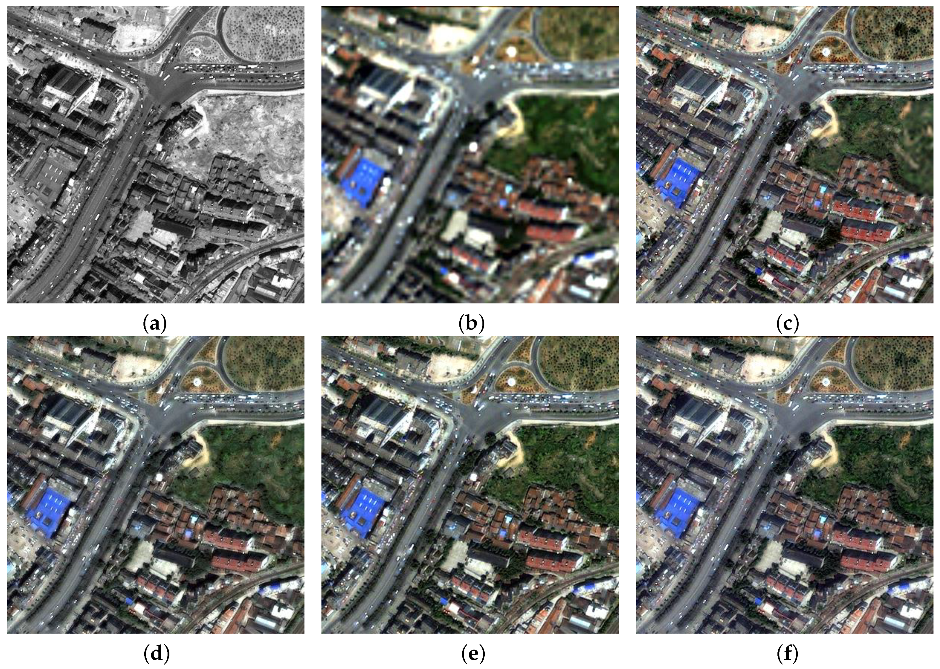
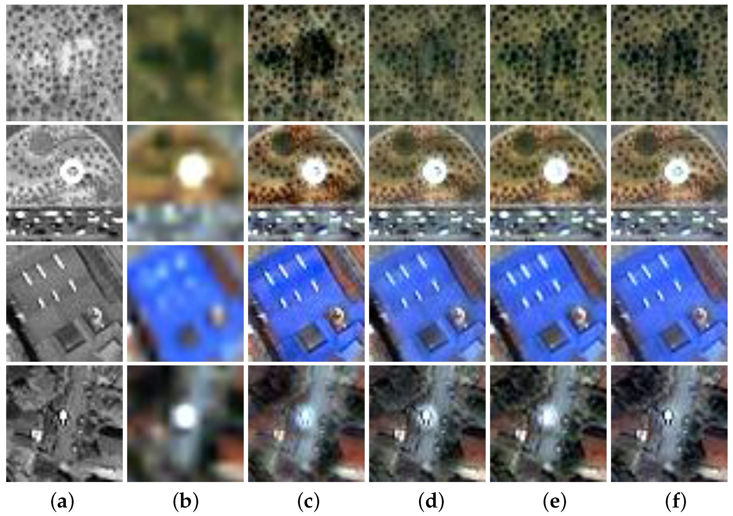
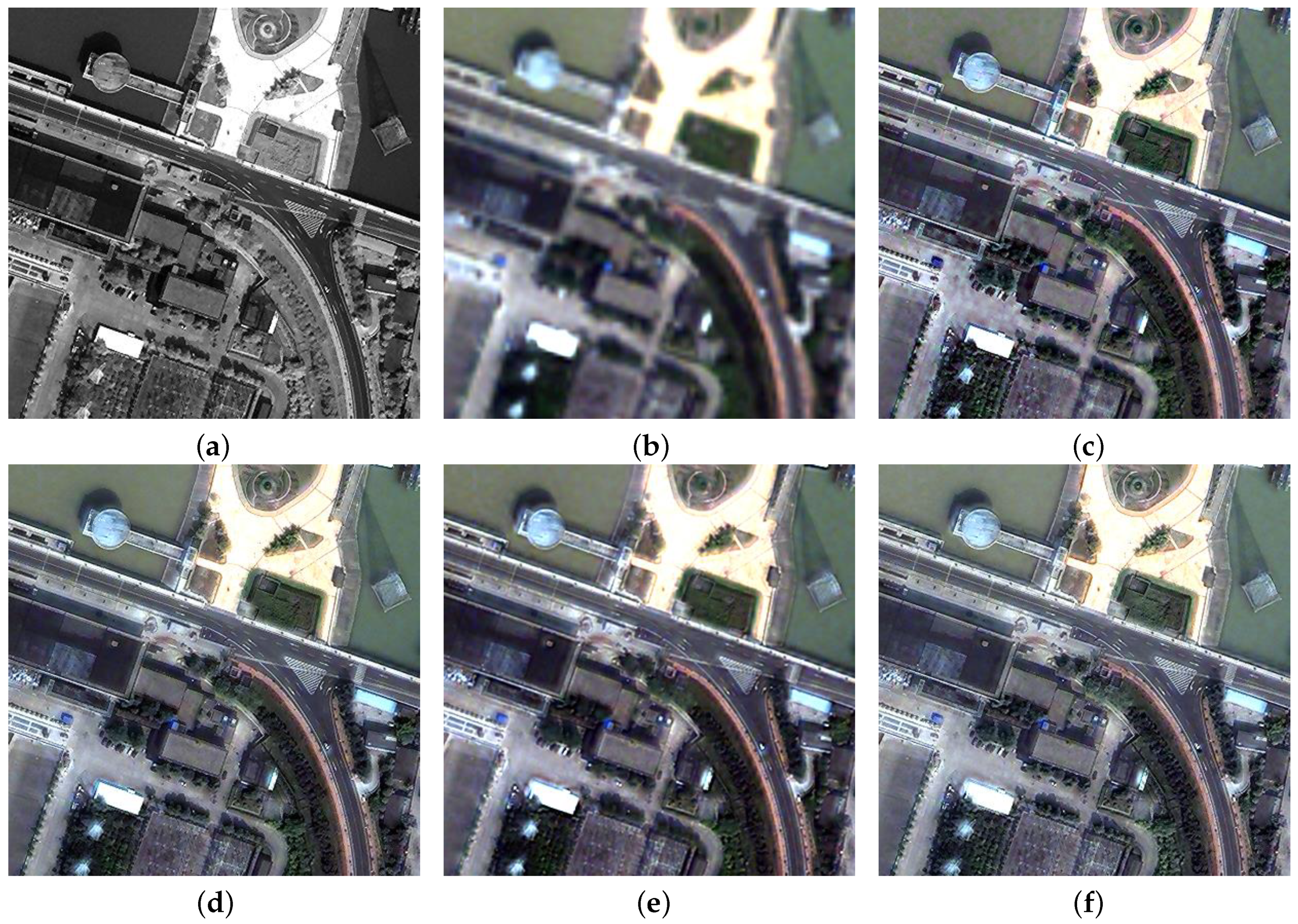
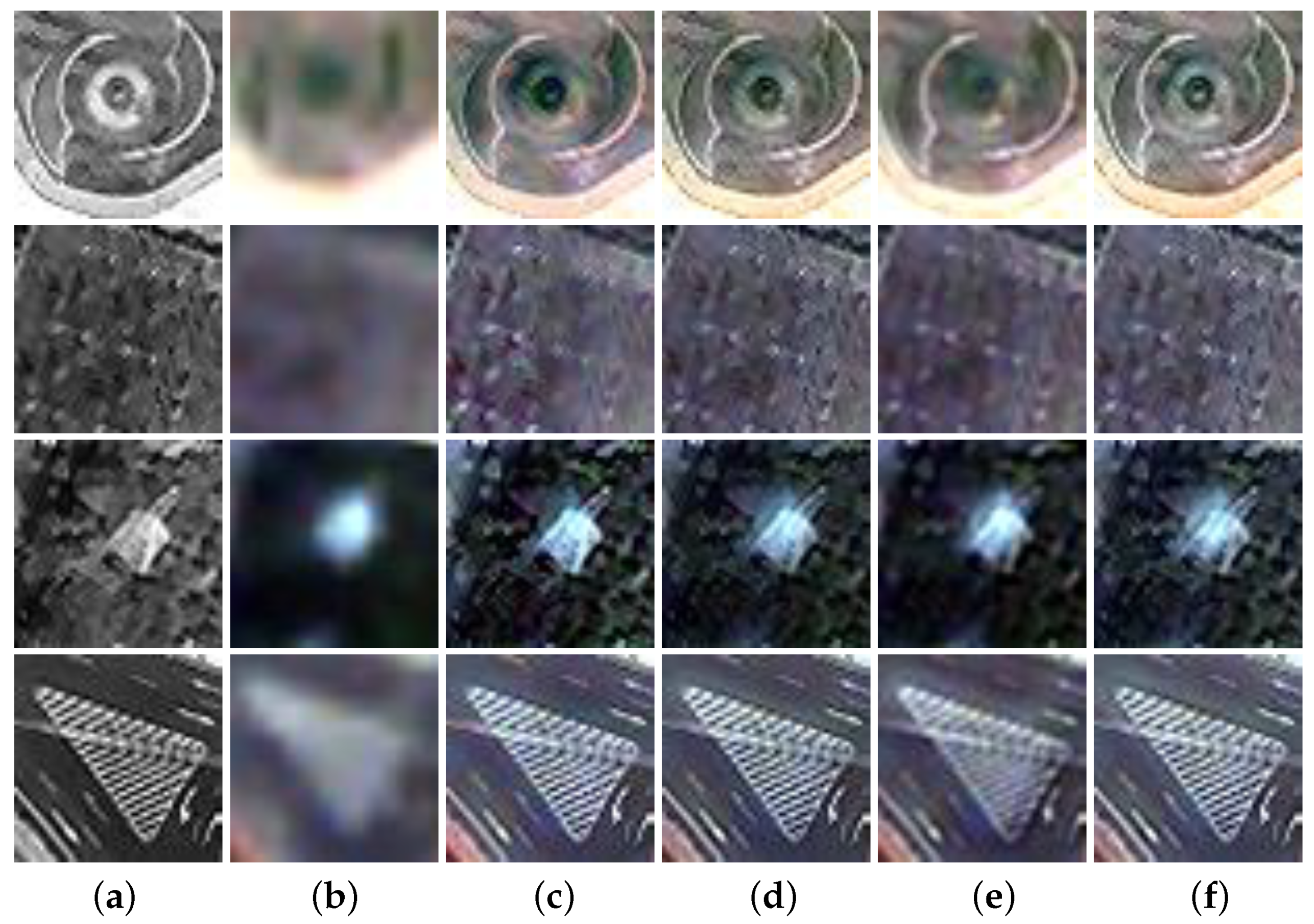
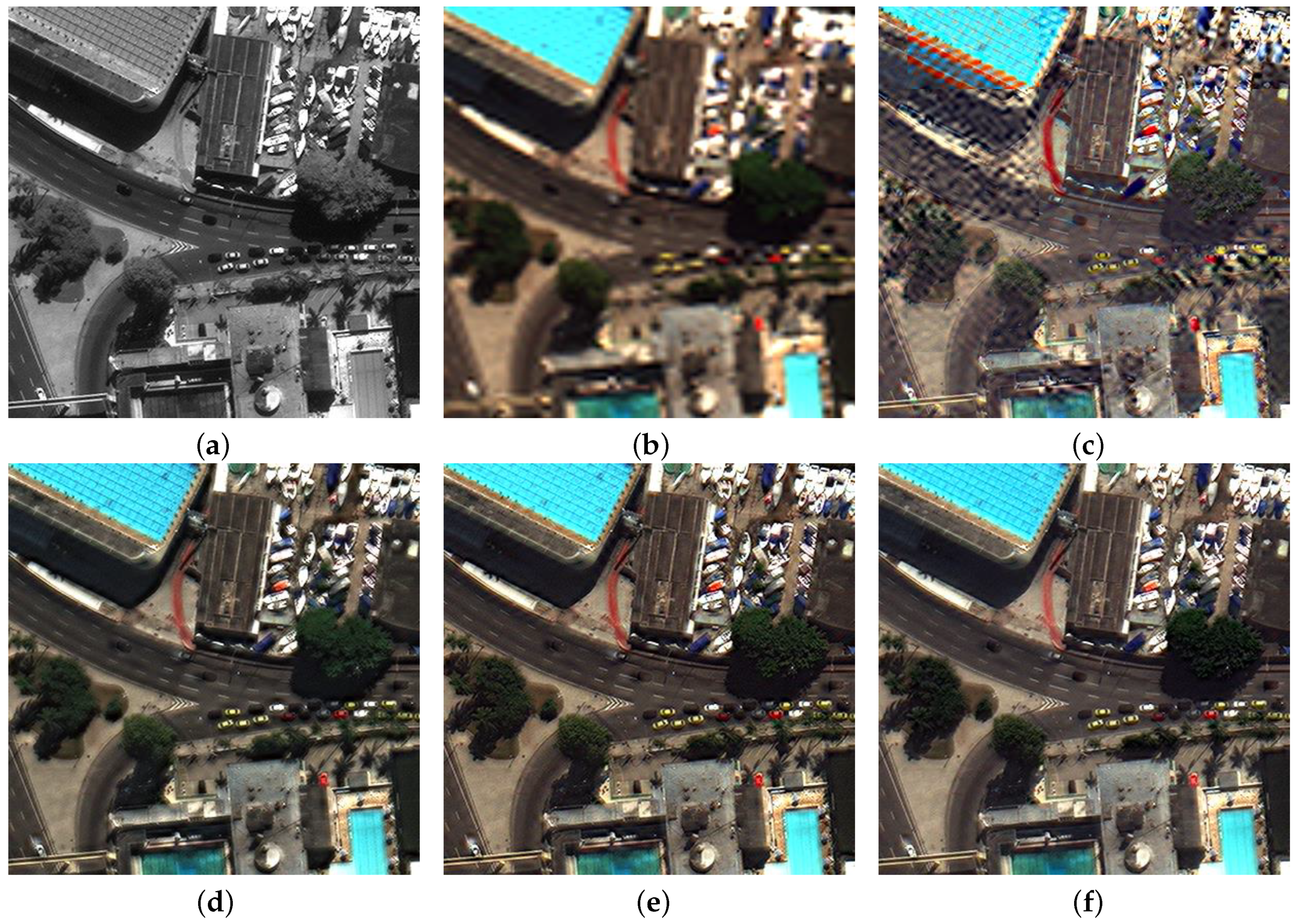
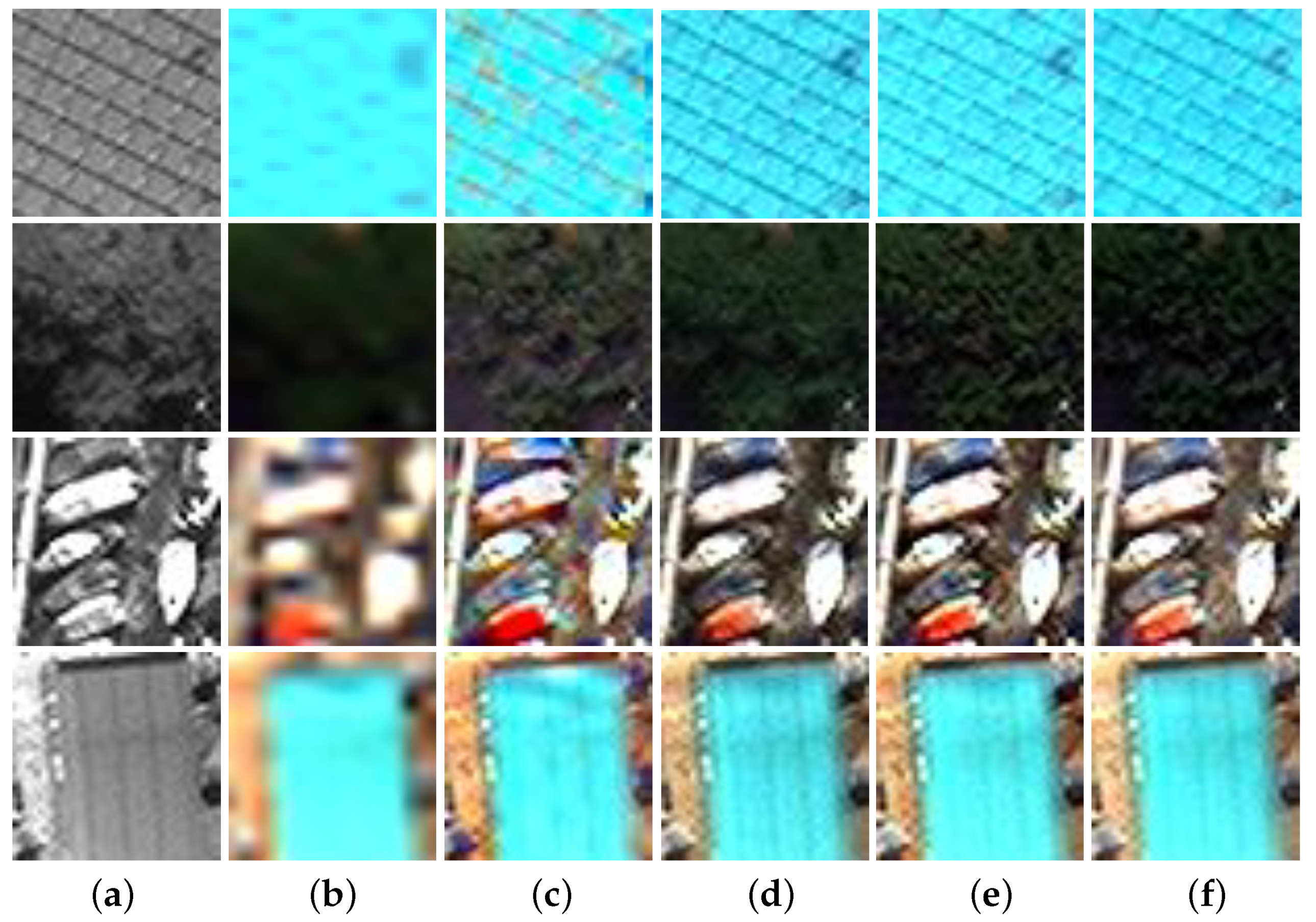
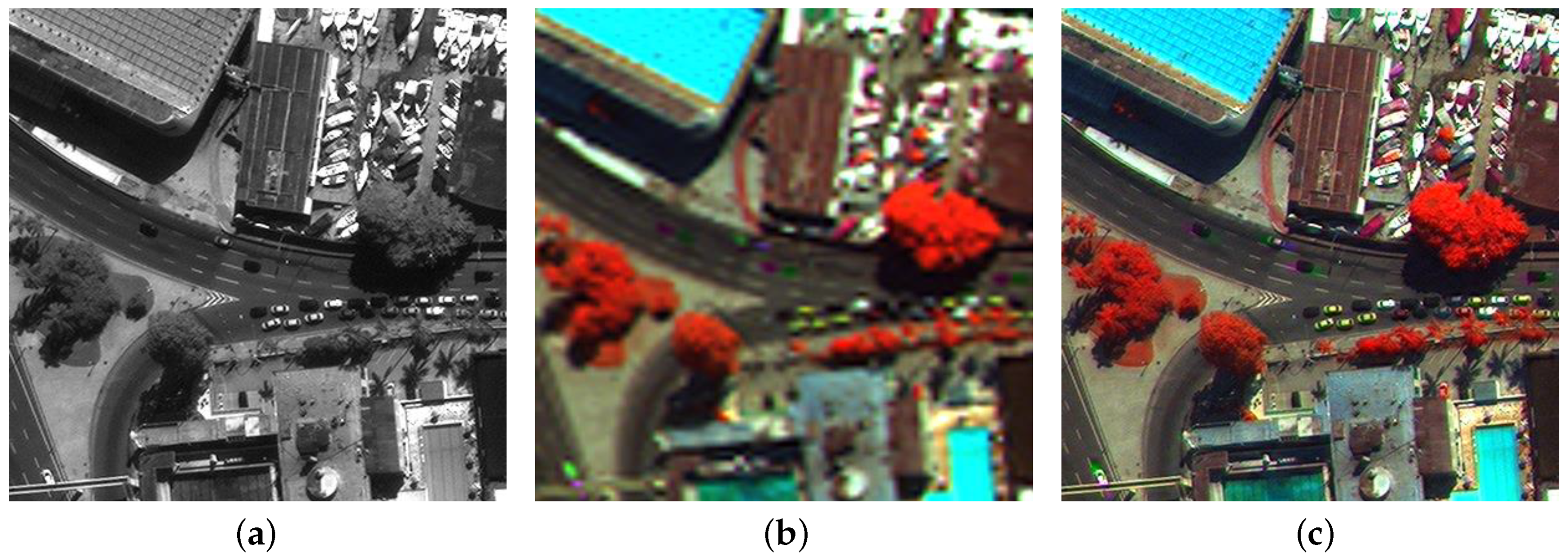
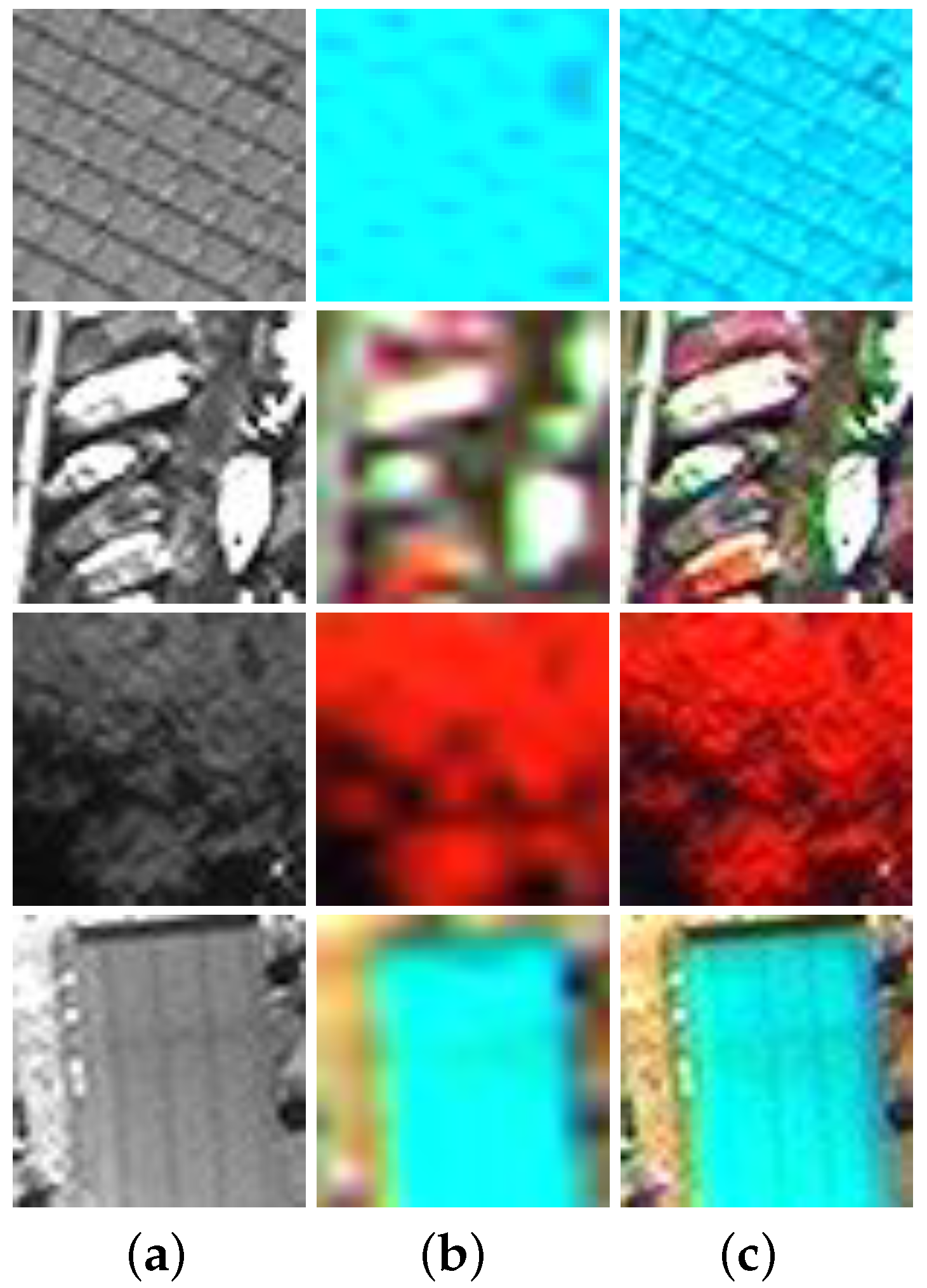
3.3. Results of IKONOS Dataset

For the original IKONOS, the data volume is 200, 20 pairs of test images in 1024 × 1024, 11,700 pairs of validation images in 128 × 128 and 46,800 pairs of training images in 128 × 128 are produced after pre-processing. The details of pre-processing are described in Section 2.4. Figure 4 is the visualization of results of BDSD, MTF-GLP-HPM-PP, PanNet, and our method. Figure 5 is its subsets to show local details. Figure 4 and Figure 5 show RGB image synthesized from red, green, and blue bands of results for comparing visual effects conveniently; (a,b) are original PAN and MS; (c–f) are the fusion result of BDSD, MTF-GLP-HPM-PP, PanNet, and our method.

Each image in Figure 4 is a partial region in size of 400 × 400 clipped from one of the test images in size of 1024 × 1024, and patches in size of 50 × 50 in Figure 5 show more details.

Figure 4 shows that our method achieves promising visual results both in spectral and spatial dimension, which can reach equal effect with the MTF-GLP-HPM-PP method and PanNet. Results of MTF-GLP-HPM-PP, PanNet, and our method have no evident spectral distortion, but some blur regions exist on results of BDSD and PanNet, especially in subsets of the second and fourth rows of (c) and (e) in Figure 5. In comparison, our method and MTF-GLP-HPM-PP show distinct spatial details, particularly details of the edges of bright objects in the subsets.

Table 4. Quality indexes of IKONOS test images.

Satellite	Method	${\mathit{D}}_{\mathit{\lambda }}$	${\mathit{D}}_{\mathit{S}}$	QNR	SAM	sCC
IKONOS	BDSD	0.025444	0.060288	0.915776	0.023733	0.586412
IKONOS	MTF-GLP-HPM-PP	0.142897	0.206561	0.682524	0.020904	0.626434
IKONOS	PanNet	0.109174	0.177450	0.735754	0.018246	0.899323
IKONOS	PDSDNet	0.118761	0.175408	0.728854	0.032151	0.608364

and Figure 6 are the values of quality indexes of results of different methods. The average value of quality indexes of these images is shown in Table 4; the dispersion of the values of quality indexes is shown by boxplot in Figure 6.

The boxplot represents the dispersion of the data through maximum, minimum, median, upper and lower quartiles of quality indexes of test images. The length of the box shows the interquartile range (IQR), and the smaller range means more concentrated data. The line’s location in the box is the median, which represents the general state of the data. Moreover, the ‘×’ is the position of mean value corresponds to the value in Table 4. The upper and lower edge line means maximum and minimum.

For IKONOS datasets, the visual effect of MTF-GLP-HPM-PP and our method are best; however, the conclusion becomes different when it comes to quantitative indicators. On no-reference indexes, the results of BDSD have the best performance as the first row shown in Figure 6. As Table 4 and Figure 6 show, the results of PanNet and our method are similar, better than MTF-GLP-HPM-PP. As for referenced indexes, PanNet shows better performance than other methods, while BDSD, MTF-GLP-HPM-PP and our method perform similarly. The results demonstrate that there is a gap between visual evaluation and quantitative evaluation.

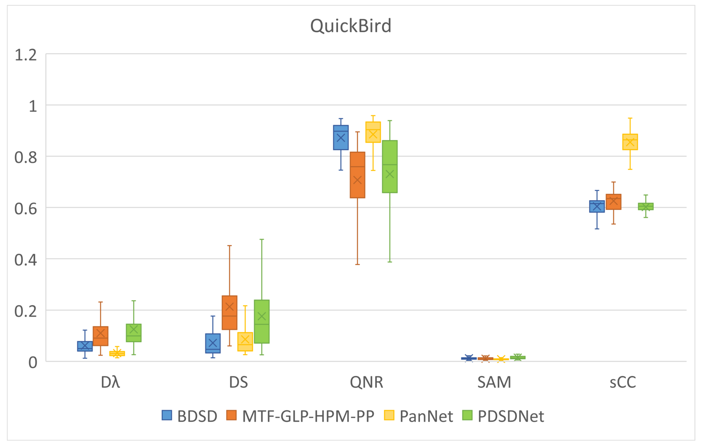
3.4. Results of QuickBird Dataset

For the original QuickBird, the data volume is 500, 50 pairs of test images in 1024 × 1024, 29,250 pairs of validation images in 128 × 128 and 117,000 pairs of training images in 128 × 128 are generated from pre-processing. Figure 7 and Figure 8 are the visualization of results of different methods on QuickBird test datasets. The third, the second, and the first band were chosen as RGB channels for visualization from four bands of QuickBird test results. The ranges of bands have been shown in Table 2. In Figure 7 and Figure 8, (a,b) are original PAN and MS, (c–f) are the fusion result of BDSD, MTF-GLP-HPM-PP, PanNet, and our method. Every image of Figure 8 is a 400 × 400 path clipped from one of 1024 × 1024 QuickBird test images or results, and 50 × 50 patches in Figure 8 show more particulars. From Figure 7, the results prove that our method also achieves superior visual results on QuickBird test images. Our method’s results still have no apparent spectral distortion and spatial distortion. Figure 8 shows that our method’s results have sharper outlines than other methods, specifically on the samples in the first row and third row. The patches of PanNet are somewhat ambiguous, and the zebra crossing on the samples in the fourth row can not be distinguished easily.

Table 5. Quality indexes of QuickBird test images.

Satellite	Method	${\mathit{D}}_{\mathit{\lambda }}$	${\mathit{D}}_{\mathit{S}}$	QNR	SAM	sCC
QuickBird	BDSD	0.061218	0.071605	0.872024	0.011920	0.604250
QuickBird	MTF-GLP-HPM-PP	0.110081	0.213027	0.707572	0.010014	0.625727
QuickBird	PanNet	0.032097	0.085783	0.885333	0.008449	0.855061
QuickBird	PDSDNet	0.124512	0.175785	0.730688	0.014147	0.602224

and Figure 9 are the values of quality indexes of different method results. The average of quantitative indicators of all QuickBird test images is shown in Table 5. Figure 9 gives the boxplot of values of quality indexes. Compared with the performance on IKONOS, our method reach closer results on QuickBird with MTF-GLP-HPM-PP method. BDSD and PanNet show similar performance on no-reference indexes. Although PanNet achieves the best results on almost all indicators in Figure 9, its visual effects are no match for MTF-GLP-HPM-PP and our method.

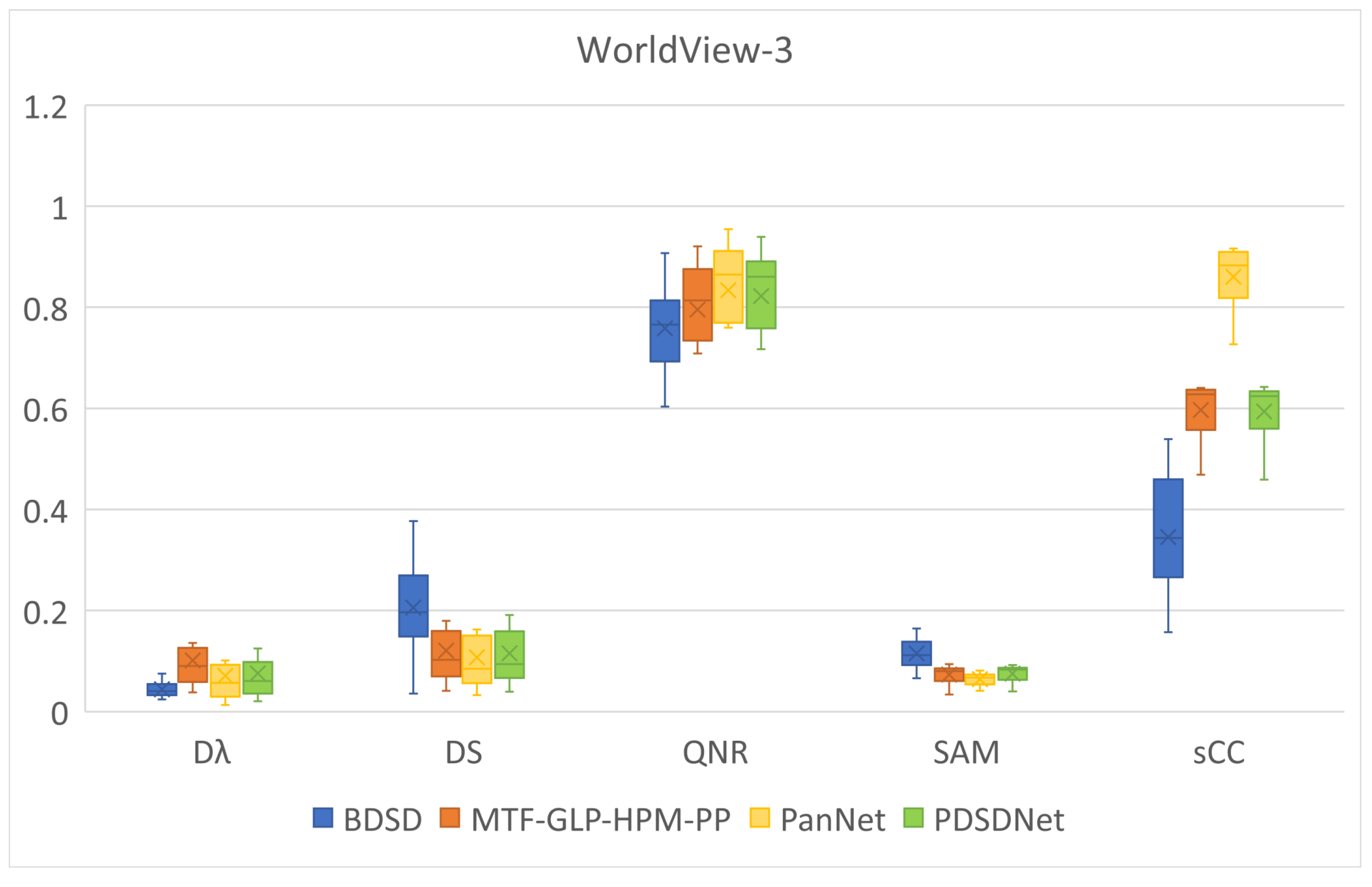
3.5. Results of WorldView-3 Dataset

In pre-processing, 16 pairs of test images in 1024 × 1024, 9360 pairs of validation images in 128 × 128, and 37,440 pairs of training images in 128 × 128 are produced from 160 original WorldView-3 images. Figure 10 and Figure 11 are the visualization of results of different methods on WorldView-3 test datasets. For convenience to facilitate the comparison of the visual effects, the fifth, third, and second band of the eight bands of WorldView-3 were combined as RGB channels for display. Figure 10 shows a 400 × 400 area on one of 1024 × 1024 WorldView-3 test images, and Figure 11 provides the local patches. As shown in Figure 7, our method also achieves outstanding visual results on WorldView-3 test images. In line with the visual effects of IKONOS and QuickBird datasets above, our method’s results have no evident spectral distortion and spatial distortion; however, the spectral preservation ability of MTF-GLP-HPM-PP method decreases. The results of BDSD suffers from severe spectral distortion, such as the architecture on BDSD result in (c) of Figure 7. Many speckles and over-saturated points arise on the whole image (c). As shown in Figure 11, BDSD method’s results have some slight mixed colors, for example, yellow or gray, especially in the first row and the third row of (c).

Table 6. Quality indexes of WorldView-3 test images.

Satellite	Method	${\mathit{D}}_{\mathit{\lambda }}$	${\mathit{D}}_{\mathit{S}}$	QNR	SAM	sCC
WorldView-3	BDSD	0.044381	0.206057	0.758531	0.115358	0.345156
WorldView-3	MTF-GLP-HPM-PP	0.101469	0.120643	0.795284	0.073263	0.597091
WorldView-3	PanNet	0.070647	0.107669	0.833849	0.064444	0.860472
WorldView-3	PDSDNet	0.075793	0.115544	0.821917	0.075176	0.593716

and Figure 12 are the values of quality indexes of different method results. The value of quantitive indicators of 16 WorldView-3 test images can be observed in Figure 12. The average of 16 images is shown in Table 6. Compared with the performance on IKONOS and QuickBird, our method also reach close results on WorldView-3 with MTF-GLP-HPM-PP, but the performance of our method becomes better on WorldView-3 than other two datasets. Compared with IKONOS and QuickBird, WorldView-3 dataset has eight bands rather than four. When the number of bands increases, quantitative indicators of PanNet’s results are still ahead overall; however, the gap in the performance of PDSDNet and PanNet decreases, while MTF-GLP-HPM-PP shows the opposite. The difference in the performance of MTF-GLP-HPM-PP and PDSDNet increases. It means that whether all bands are utilized for simulating low-resolution PAN will have an influence on fusion results when some multispectral bands have no intersection with the panchromatic band in wavelength.

For only six bands participating in learning the simulated PAN in PDSDNet, but with the details being added to all bands, we select the eighth, third, and first band for false color composite (FCC) to observe the effect in Figure 13. The eighth band and the first band were not involved in simulating PAN. The details are shown in Figure 14, and the first row from left to right is PAN, FCC of MS, and FCC of PDSDNet result, then the second and the third row is four groups of local details of the first row images. No obvious spectral or spatial distortion appears in visualization, although the two bands have not participated in the network of producing filters.

4. Discussion

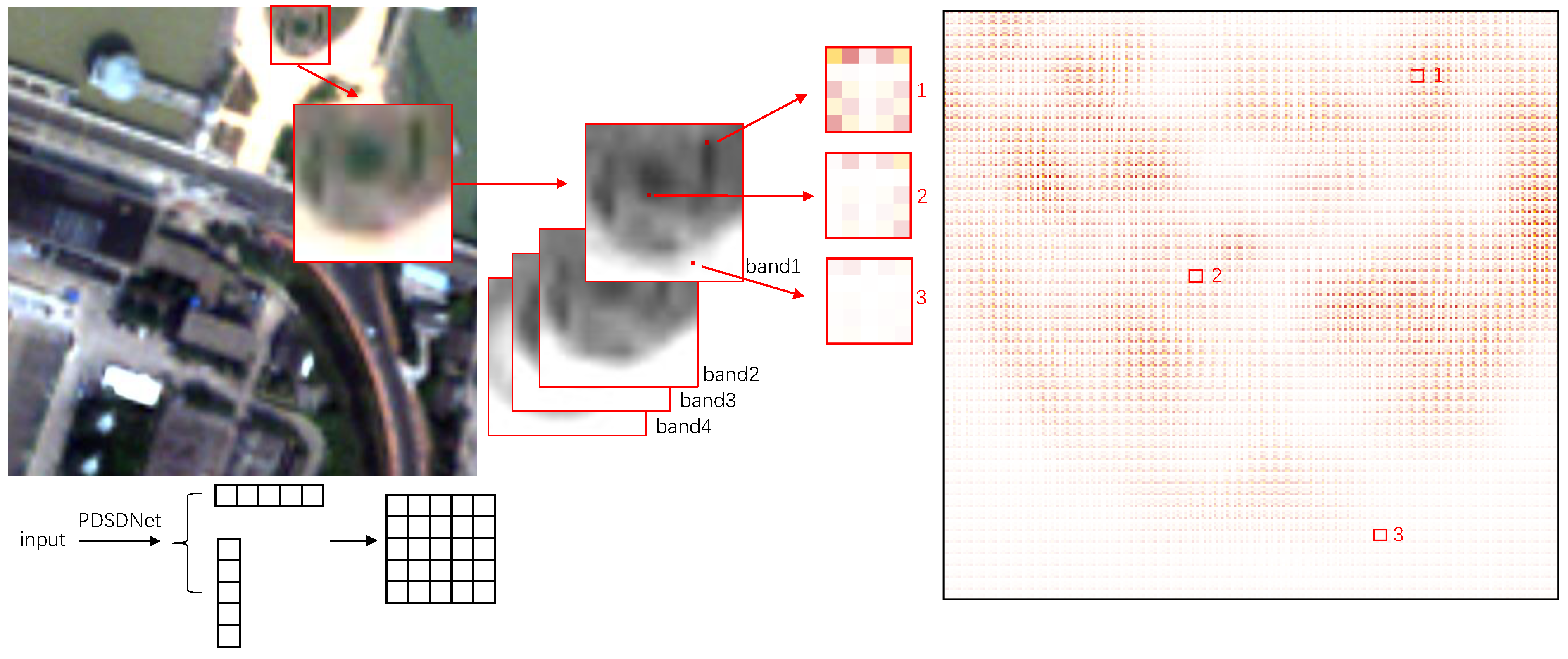
4.1. Visualization of Filters

In order to validate whether it is necessary for the adaptive filter network to generate a set of convolution kernels for each pixel instead of sharing the convolution kernels for the full image, we select a test image and output its filter after the simulating network. For convenience for the visualization, we multiply two single-dimensional filters together, so each pixel corresponds to one 5 × 5 kernel, then tile kernels according to the pixel location. The heat map of this matrix was drawn, and 250 × 250 area on the map is shown in Figure 15 for observing, which corresponds to the 50 × 50 local test patch. The deeper red represents the bigger value, and the greater yellow denotes the smaller value. When the value is close to the middle of the 250 × 250 data distribution, the map shows white. From Figure 15, it is clear that filters of different pixels have significant differences, which are related to the edges of the object.

4.2. Comparative Analysis of Methods

We have conducted experiments on IKONOS, QuickBird, and WorldView-3 datasets with BDSD, MTF-GLP-HPM-PP, PanNet, and PDSDNet. Visualization and quantitative evaluation of the results of four methods on three datasets with five indexes have been shown. Figure 4, Figure 7, and Figure 10 demonstrate a whole effect of 400 × 400 areas where spectral preservation can be observed. Figure 5, Figure 8, and Figure 11 focus on the local details of 50 × 50 areas. Figure 6, Figure 9, and Figure 12 show the data distribution of the quantitative indicators of the results. Table 4, Table 5 and Table 6 show the average value of the quantitative indicators of the results. Figure 13 and Figure 14 show the performance of the proposed method on WorldView-3 dataset in the Coastal and NIR2 band, which are not involved in simulating panchromatic image. Figure 15 shows the visualization of filters corresponding to part of pixels of one band generated by the proposed method in this paper.

From the above results of the three datasets, the visual effect of our method is promising with no conspicuous spectral distortion. The results of the proposed method indicate that the spectral effect of simulating PAN obtained by the combination of MS bands is relatively close to the real PAN. The proposed method in this paper assumes that if the resolution of panchromatic and multispectral images are consistent, the panchromatic band has the same details as each multispectral band; therefore, the spatial detail is identical for each band when the details obtained from the real PAN and simulating PAN are infused to the upsampled MS. The visualization of the two other bands in the eight-band dataset presents as much detail as the others without spatial distortion. It is consistent with the previous assumption. The results showed no evident spatial distortion in the local patches. Compared with other methods, the visual effect of the proposed method demonstrates more advantages.

In terms of quantitative indicators, the results of the proposed method are not the most outstanding on the three datasets among the four methods, but no significant difference exists between our method and the best or second-best method most of the time. The quantitative performance may be related to the perspective of measurement. Although the results of BDSD are block-fuzzy, BDSD performs well in the no-reference quantitative indexes on IKONOS dataset and QuickBird dataset. The values of quantitative indicators of PanNet’s results are positive, but detailed information is not abundant enough with fuzzy edge in visual. It indicates that the performance of quantitative indexes could be inconsistent with the visual effect. Whether the method is local optimal or global optimal, and whether the index is calculated by averaging the values of the local areas or measured in pixels, may affect the evaluation of the method in terms of the index.

5. Conclusions

In this paper, a pixel-dependent spatial-detail injection network (PDSDNet) is proposed. Based on the dynamic filter network, PDSDNet constructs the nonlinear mapping of the simulated panchromatic band from the low-resolution multispectral band through filter convolution regression. On the one hand, PDSDNet reduces the possibility of spectral distortion and spatial distortion by improving the similarity between the simulated panchromatic band and the real panchromatic band. On the other hand, the pansharpened images have rich spatial details, assuming that the panchromatic band has the same spatial details as each multispectral band.

The experimental results show that PDSDNet can generated high-quality fusion image with multi-resolution images and panchromatic images. The comparison between the proposed method and the widely utilized methods BDSD, MTF-GLP-HPM-PP, PanNet of pansharpening on IKONOS, QuickBird, and WorldView-3 datasets demonstrates that the proposed network presents superior visual effects without noticeable spectral distortion and spatial distortion. The quality indexes show that the PDSDNet only obtain result in approximate level similar to the MTF-GLP-HPM-PP’s results, not the best one.

Our experimental results demonstrate that quantitative indicators in the evaluation do not match the expected visual evaluation outcomes. It is not a novel finding. Devising new quantitative indicators that match the human perceptual assessment is still an open research problem in image fusion.

Although the proposed method has superior fusion visual performance, quantitative results are not outstanding enough. In fact, in this paper, quantitative indicators were applied to evaluate fusion images, but the optimization in PDSDNet is to simulate panchromatic band. In future work, we will explore establishing a pixel-dependent spatial-detail injection model on dynamic filter networks to obtain both promising visual and quantitative results.

References

1. Tu, T.M.; Su, S.C.; Shyu, H.C.; Huang, P.S. A new look at IHS-like image fusion methods. Inf. Fusion 2001, 2, 177–186. [Google Scholar] [CrossRef]
2. Koutsias, N.; Karteris, M.; Chuvieco, E. The Use of Intensity-Hue-Saturation Transformation of Landsat5 Thematic Mapper Data for Burned Land Mapping. Photogramm. Eng. Remote Sens. 2000, 66, 829–839. [Google Scholar]
3. Rahmani, S.; Strait, M.; Merkurjev, D.; Moeller, M.; Wittman, T. An Adaptive IHS Pan-Sharpening Method. IEEE Geosci. Remote Sens. Lett. 2010, 7, 746–750. [Google Scholar] [CrossRef] [Green Version]
4. Gonzalez-Audicana, M.; Saleta, J.; Catalan, R.; Garcia, R. Fusion of multispectral and panchromatic images using improved IHS and PCA mergers based on wavelet decomposition. IEEE Trans. Geosci. Remote Sens. 2004, 42, 1291–1299. [Google Scholar] [CrossRef]
5. Gillespie, A.R.; Kahle, A.B.; Walker, R.E. Color enhancement of highly correlated images. II. Channel ratio and “chromaticity” transformation techniques. Remote Sens. Environ. 1987, 22, 343–365. [Google Scholar] [CrossRef]
6. Maurer, T. How to pan-sharpen images using the Gram-Schmidt pan-sharpen method—A recipe. ISPRS-Int. Arch. Photogramm. Remote Sens. Spat. Inf. Sci. 2013, XL-1/W1, 239–244. [Google Scholar] [CrossRef] [Green Version]
7. Aiazzi, B.; Baronti, S.; Selva, M. Improving Component Substitution Pansharpening Through Multivariate Regression of MS +Pan Data. IEEE Trans. Geosci. Remote Sens. 2007, 45, 3230–3239. [Google Scholar] [CrossRef]
8. Chavez, P., Jr.; Kwarteng, A. Extracting spectral contrast in Landsat Thematic Mapper image data using selective principal component analysis. Photogramm. Eng. Remote Sens. 1989, 55, 339–348. [Google Scholar]
9. Chavez, P.S., Jr.; Sides, S.C.; Anderson, J.A. Comparison of three different methods to merge multiresolution and multispectral data: LANDSAT TM and SPOT panchromatic. Photogramm. Eng. Remote Sens. 1991, 57, 265–303. [Google Scholar]
10. Garzelli, A.; Nencini, F.; Capobianco, L. Optimal MMSE Pan Sharpening of Very High Resolution Multispectral Images. IEEE Trans. Geosci. Remote Sens. 2008, 46, 228–236. [Google Scholar] [CrossRef]
11. Choi, J.; Yu, K.; Kim, Y. A New Adaptive Component-Substitution-Based Satellite Image Fusion by Using Partial Replacement. IEEE Trans. Geosci. Remote Sens. 2011, 49, 295–309. [Google Scholar] [CrossRef]
12. Otazu, X.; González-Audicana, M.; Fors, O.; Murga, J. Introduction of Sensor Spectral Response into Image Fusion Methods. Application to Wavelet-Based Methods. IEEE Trans. Geosci. Remote Sens. 2005, 43, 2376–2385. [Google Scholar] [CrossRef] [Green Version]
13. Nason, G.; Silverman, B. The Stationary Wavelet Transform and some Statistical Applications. In Wavelets and Statistics; Lecture Notes in Statistics; Springer: New York, NY, USA, 1995; pp. 281–300. [Google Scholar] [CrossRef]
14. Mallat, S. A theory for multiresolution signal decomposition: The wavelet representation. IEEE Trans. Pattern Anal. Mach. Intell. 1989, 11, 674–693. [Google Scholar] [CrossRef] [Green Version]
15. Khan, M.M.; Chanussot, J.; Condat, L.; Montanvert, A. Indusion: Fusion of Multispectral and Panchromatic Images Using the Induction Scaling Technique. IEEE Geosci. Remote Sens. Lett. 2008, 5, 98–102. [Google Scholar] [CrossRef] [Green Version]
16. Shensa, M. The discrete wavelet transform: Wedding the a trous and Mallat algorithms. IEEE Trans. Signal Process. 1992, 40, 2464–2482. [Google Scholar] [CrossRef] [Green Version]
17. Ranchin, T.; Wald, L. Fusion of high spatial and spectral resolution images: The ARSIS concept and its implementation. Photogramm. Eng. Remote Sens. 2000, 66, 49–61. [Google Scholar]
18. Nunez, J.; Otazu, X.; Fors, O.; Prades, A.; Pala, V.; Arbiol, R. Multiresolution-based image fusion with additive wavelet decomposition. IEEE Trans. Geosci. Remote Sens. 1999, 37, 1204–1211. [Google Scholar] [CrossRef] [Green Version]
19. Burt, P.J.; Adelson, E.H. The Laplacian Pyramid as a Compact Image Code. In Readings in Computer Vision; Fischler, M.A., Firschein, O., Eds.; Morgan Kaufmann: San Francisco, CA, USA, 1987; pp. 671–679. [Google Scholar] [CrossRef]
20. Aiazzi, B.; Alparone, L.; Baronti, S.; Garzelli, A.; Selva, M. MTF-tailored Multiscale Fusion of High-resolution MS and Pan Imagery. Photogramm. Eng. Remote Sens. 2006, 72, 591–596. [Google Scholar] [CrossRef]
21. Vivone, G.; Restaino, R.; Dalla Mura, M.; Licciardi, G.; Chanussot, J. Contrast and Error-Based Fusion Schemes for Multispectral Image Pansharpening. IEEE Geosci. Remote Sens. Lett. 2014, 11, 930–934. [Google Scholar] [CrossRef] [Green Version]
22. Lee, J.; Lee, C. Fast and Efficient Panchromatic Sharpening. IEEE Trans. Geosci. Remote Sens. 2010, 48, 155–163. [Google Scholar] [CrossRef]
23. Huang, W.; Xiao, L.; Wei, Z.; Liu, H.; Tang, S. A New Pan-Sharpening Method with Deep Neural Networks. IEEE Geosci. Remote Sens. Lett. 2015, 12, 1037–1041. [Google Scholar] [CrossRef]
24. Dong, C.; Loy, C.C.; He, K.; Tang, X. Image Super-Resolution Using Deep Convolutional Networks. IEEE Trans. Pattern Anal. Mach. Intell. 2016, 38, 295–307. [Google Scholar] [CrossRef] [PubMed] [Green Version]
25. Masi, G.; Cozzolino, D.; Verdoliva, L.; Scarpa, G. Pansharpening by Convolutional Neural Networks. Remote Sens. 2016, 8, 594. [Google Scholar] [CrossRef] [Green Version]
26. Wei, Y.; Yuan, Q.; Shen, H.; Zhang, L. Boosting the Accuracy of Multispectral Image Pansharpening by Learning a Deep Residual Network. IEEE Geosci. Remote Sens. Lett. 2017, 14, 1795–1799. [Google Scholar] [CrossRef] [Green Version]
27. Yuan, Q.; Wei, Y.; Meng, X.; Shen, H.; Zhang, L. A Multiscale and Multidepth Convolutional Neural Network for Remote Sensing Imagery Pan-Sharpening. IEEE J. Sel. Top. Appl. Earth Obs. Remote Sens. 2018, 11, 978–989. [Google Scholar] [CrossRef] [Green Version]
28. Yang, J.; Fu, X.; Hu, Y.; Huang, Y.; Ding, X.; Paisley, J. PanNet: A Deep Network Architecture for Pan-Sharpening. In Proceedings of the 2017 IEEE International Conference on Computer Vision (ICCV), Venice, Italy, 22–29 October 2017; pp. 1753–1761. [Google Scholar] [CrossRef]
29. Scarpa, G.; Vitale, S.; Cozzolino, D. Target-Adaptive CNN-Based Pansharpening. IEEE Trans. Geosci. Remote Sens. 2018, 56, 5443–5457. [Google Scholar] [CrossRef] [Green Version]
30. Vitale, S.; Scarpa, G. A Detail-Preserving Cross-Scale Learning Strategy for CNN-Based Pansharpening. Remote Sens. 2020, 12, 348. [Google Scholar] [CrossRef] [Green Version]
31. Shao, Z.; Cai, J. Remote Sensing Image Fusion With Deep Convolutional Neural Network. IEEE J. Sel. Top. Appl. Earth Obs. Remote Sens. 2018, 11, 1656–1669. [Google Scholar] [CrossRef]
32. Goodfellow, I.; Pouget-Abadie, J.; Mirza, M.; Xu, B.; Warde-Farley, D.; Ozair, S.; Courville, A.; Bengio, Y. Generative Adversarial Networks. In Proceedings of the Advances in Neural Information Processing Systems, Montreal, QC, Canada, 8–13 October 2014; Volume 27. [Google Scholar] [CrossRef]
33. Liu, Q.; Zhou, H.; Xu, Q.; Liu, X.; Wang, Y. PSGAN: A Generative Adversarial Network for Remote Sensing Image Pan-Sharpening. IEEE Trans. Geosci. Remote Sens. 2021, 59, 10227–10242. [Google Scholar] [CrossRef]
34. Shao, Z.; Lu, Z.; Ran, M.; Fang, L.; Zhou, J.; Zhang, Y. Residual Encoder–Decoder Conditional Generative Adversarial Network for Pansharpening. IEEE Geosci. Remote Sens. Lett. 2020, 17, 1573–1577. [Google Scholar] [CrossRef]
35. Ma, J.; Yu, W.; Chen, C.; Liang, P.; Guo, X.; Jiang, J. Pan-GAN: An unsupervised pan-sharpening method for remote sensing image fusion. Inf. Fusion 2020, 62, 110–120. [Google Scholar] [CrossRef]
36. Ozcelik, F.; Alganci, U.; Sertel, E.; Unal, G. Rethinking CNN-Based Pansharpening: Guided Colorization of Panchromatic Images via GANs. IEEE Trans. Geosci. Remote Sens. 2021, 59, 3486–3501. [Google Scholar] [CrossRef]
37. Liu, X.; Liu, Q.; Wang, Y. Remote sensing image fusion based on two-stream fusion network. Inf. Fusion 2020, 55, 1–15. [Google Scholar] [CrossRef] [Green Version]
38. Jia, X.; De Brabandere, B.; Tuytelaars, T.; Gool, L.V. Dynamic Filter Networks. In Proceedings of the Advances in Neural Information Processing Systems, Barcelona, Spain, 5–10 December 2016; Volume 29. [Google Scholar]
39. Niklaus, S.; Mai, L.; Liu, F. Video Frame Interpolation via Adaptive Separable Convolution. In Proceedings of the IEEE International Conference on Computer Vision (ICCV), Venice, Italy, 22–29 October 2017. [Google Scholar]
40. Niklaus, S.; Mai, L.; Liu, F. Video Frame Interpolation via Adaptive Convolution. In Proceedings of the IEEE Conference on Computer Vision and Pattern Recognition (CVPR), Honolulu, HI, USA, 21–26 July 2017. [Google Scholar]
41. Jin, X.; Tang, P.; Zhang, Z. Sequence Image Datasets Construction via Deep Convolution Networks. Remote Sens. 2021, 13, 1853. [Google Scholar] [CrossRef]
42. Meng, X.; Xiong, Y.; Shao, F.; Shen, H.; Sun, W.; Yang, G.; Yuan, Q.; Fu, R.; Zhang, H. A Large-Scale Benchmark Data Set for Evaluating Pansharpening Performance: Overview and Implementation. IEEE Geosci. Remote Sens. Mag. 2021, 9, 18–52. [Google Scholar] [CrossRef]
43. Aiazzi, B.; Alparone, L.; Baronti, S.; Garzelli, A. Context-driven fusion of high spatial and spectral resolution data based on oversampled multiresolution analysis. IEEE Trans. Geosci. Remote Sens. 2002, 40, 2300–2312. [Google Scholar] [CrossRef]
44. Aiazzi, B.; Alparone, L.; Baronti, S.; Garzelli, A.; Selva, M. An MTF-based spectral distortion minimizing model for pan-sharpening of very high resolution multispectral images of urban areas. In Proceedings of the 2003 2nd GRSS/ISPRS Joint Workshop on Remote Sensing and Data Fusion over Urban Areas, Berlin, Germany, 22–23 May 2003; pp. 90–94. [Google Scholar] [CrossRef]
45. Aiazzi, B.; Alparone, L.; Baronti, S.; Carlà, R.; Garzelli, A.; Santurri, L. Full scale assessment of pansharpening methods and data products. Proc. SPIE- Int. Soc. Opt. Eng. 2014, 9244, 924402. [Google Scholar] [CrossRef]
46. Alparone, L.; Aiazzi, B.; Baronti, S.; Garzelli, A.; Nencini, F.; Selva, M. Multispectral and Panchromatic Data Fusion Assessment Without Reference. ASPRS J. Photogramm. Eng. Remote Sens. 2008, 74, 193–200. [Google Scholar] [CrossRef] [Green Version]
47. Yuhas, R.H.; Goetz, A.; Boardman, J. Discrimination among Semi-Arid Landscape Endmembers Using the Spectral Angle Mapper (SAM) Algorithm. In Proceedings of the Summaries of the Third Annual JPL Airborne Geoscience Workshop, Pasadena, CA, USA, 1–5 June 1992; Volume 1, pp. 147–149. [Google Scholar]
48. Zhou, J.; Civco, D.L.; Silander, J.A. A wavelet transform method to merge Landsat TM and SPOT panchromatic data. Int. J. Remote Sens. 1998, 19, 743–757. [Google Scholar] [CrossRef]
49. Wang, Z.; Bovik, A. A universal image quality index. IEEE Signal Process. Lett. 2002, 9, 81–84. [Google Scholar] [CrossRef]
Figure 1. Spectral response of the QuickBird panchromatic and multispectral imagery.
Remotesensing 14 01242 g001
Figure 2. The structure of PDSDNet, which inputs four bands MS and outputs filters for simulating PAN.
Remotesensing 14 01242 g002
Figure 3. The process of our fusion method.
Remotesensing 14 01242 g003
Figure 4. Visualization of IKONOS test image: (a) PAN; (b) MS; (c) BDSD; (d) MTF-GLP-HPM-PP; (e) PanNet; (f) PDSDNet.
Remotesensing 14 01242 g004
Figure 5. Visualization of local details of IKONOS test image: (a) PAN; (b) MS; (c) BDSD; (d) MTF-GLP-HPM-PP; (e) PanNet; (f) PDSDNet.
Remotesensing 14 01242 g005
Figure 6. Quality indexes of results of BDSD, MTF-GLP-HPM-PP, PanNet, and PDSDNet.
Remotesensing 14 01242 g006
Figure 7. Visualization of QuickBird test images: (a) PAN; (b) MS; (c) BDSD; (d) MTF-GLP-HPM-PP; (e) PanNet; (f) PDSDNet.
Remotesensing 14 01242 g007
Figure 8. Visualization of local details of QuickBird test images: (a) PAN; (b) MS; (c) BDSD; (d) MTF-GLP-HPM-PP; (e) PanNet; (f) PDSDNet.
Remotesensing 14 01242 g008
Figure 9. Quality indexes of results of BDSD, MTF-GLP-HPM-PP, PanNet, and PDSDNet.
Remotesensing 14 01242 g009
Figure 10. Visualization of WorldView-3 test images: (a) PAN; (b) MS; (c) BDSD; (d) MTF-GLP-HPM-PP; (e) PanNet; (f) PDSDNet.
Remotesensing 14 01242 g010
Figure 11. Visualization of local details of WorldView-3 test images: (a) PAN; (b) MS; (c) BDSD; (d) MTF-GLP-HPM-PP; (e) PanNet; (f) PDSDNet.
Remotesensing 14 01242 g011
Figure 12. Quality indexes of results of BDSD, MTF-GLP-HPM-PP, PanNet, and PDSDNet.
Remotesensing 14 01242 g012
Figure 13. (a) PAN; (b,c) the eighth, the third, and the first band for false color composite; (b) MS; (c) PDSDNet.
Remotesensing 14 01242 g013
Figure 14. Local details: (a) PAN; (b,c) the eighth, the third, and the first band for false color composite; (b) MS; (c) PDSDNet.
Remotesensing 14 01242 g014
Figure 15. The heat map of the PDSDNet filters corresponding to the first row test image in Figure 8.
Remotesensing 14 01242 g015