
A Planted Forest Mapping Method Based on Long-Term Change Trend Features Derived from Dense Landsat Time Series in an Ecological Restoration Region


Abstract
:1. Introduction
2. Materials and Methods
2.1. Materials
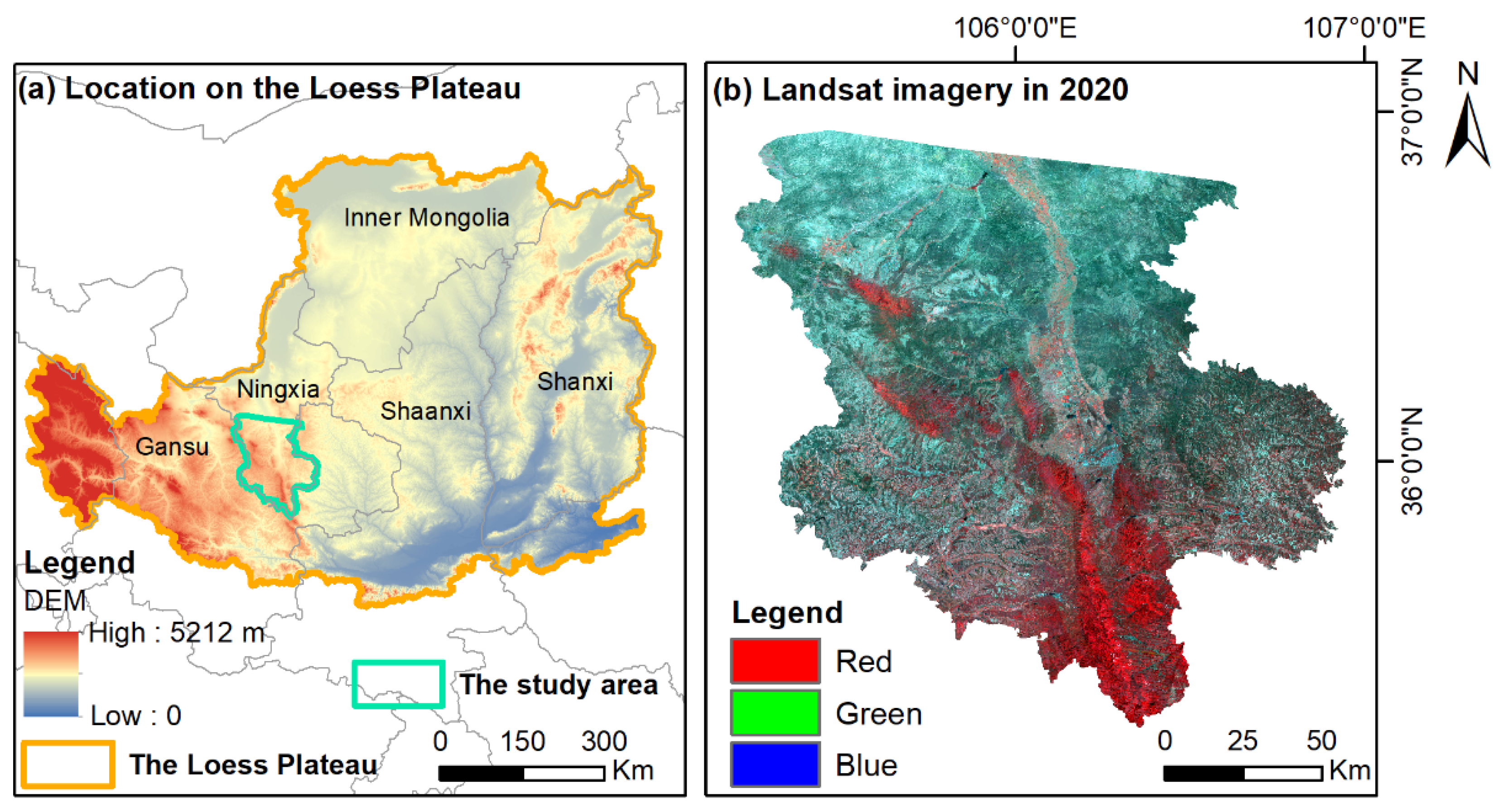
2.1.1. Study Area
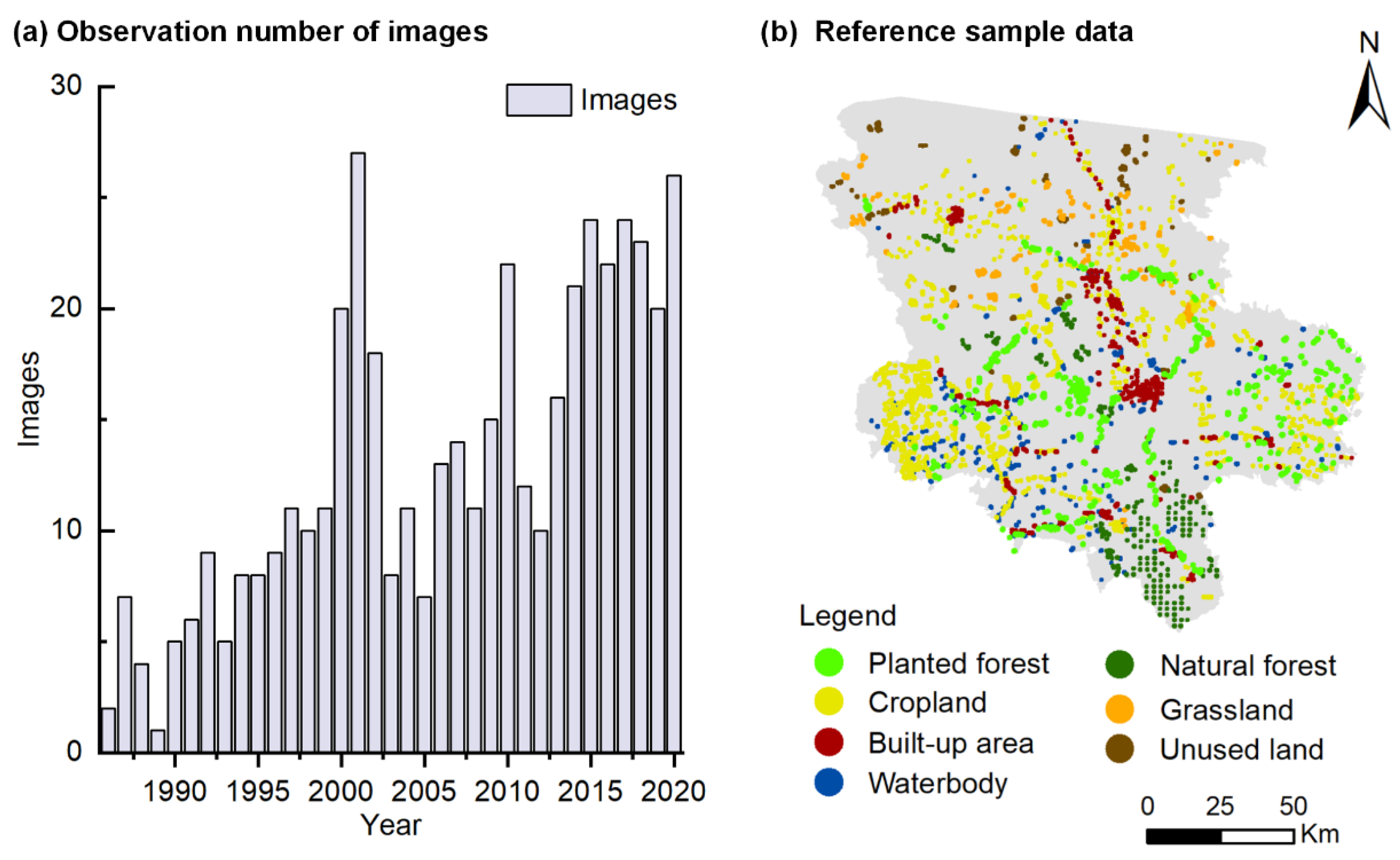
2.1.2. Landsat Time Series Processing
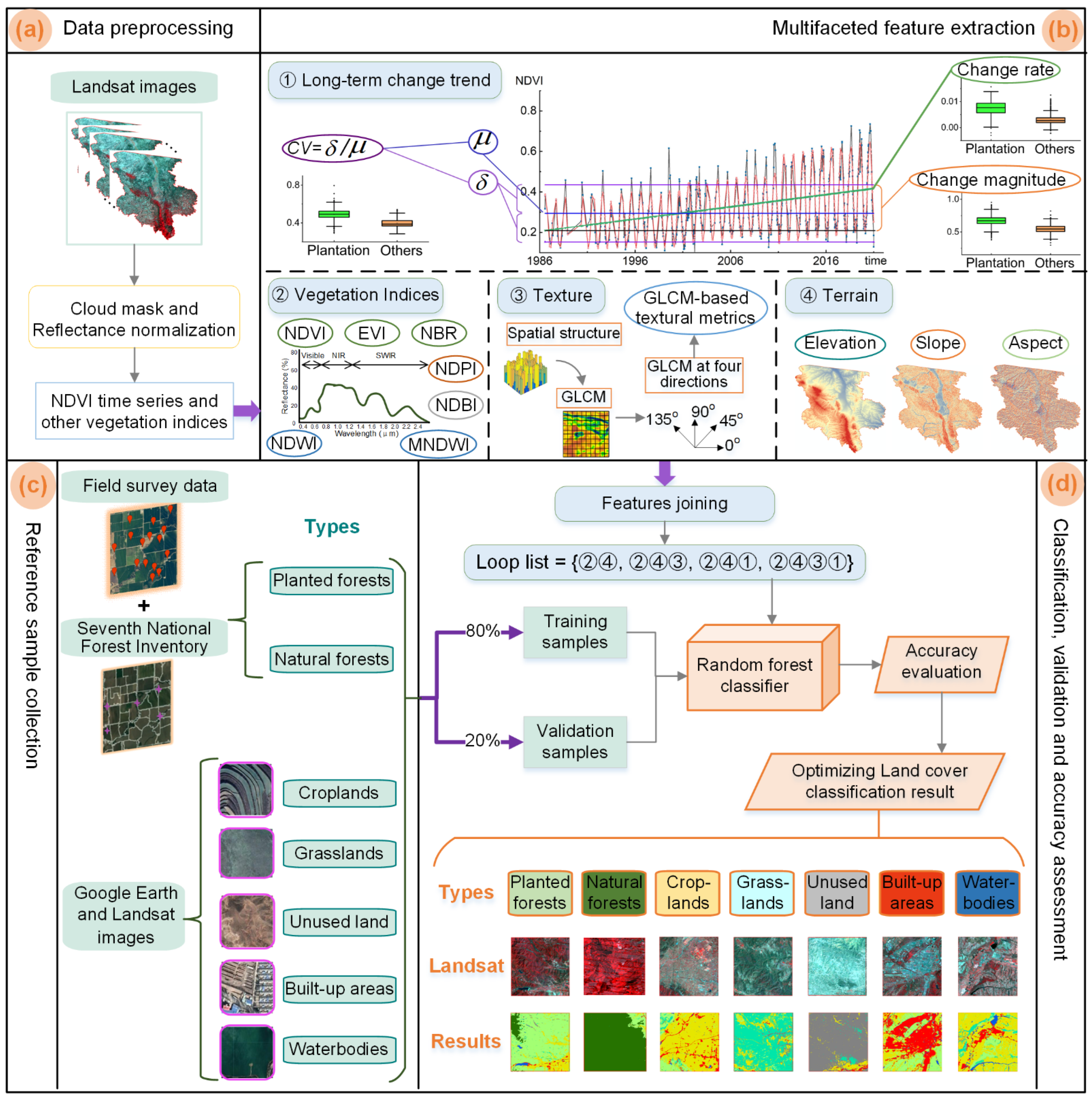
2.2. Multifaceted Feature Extraction
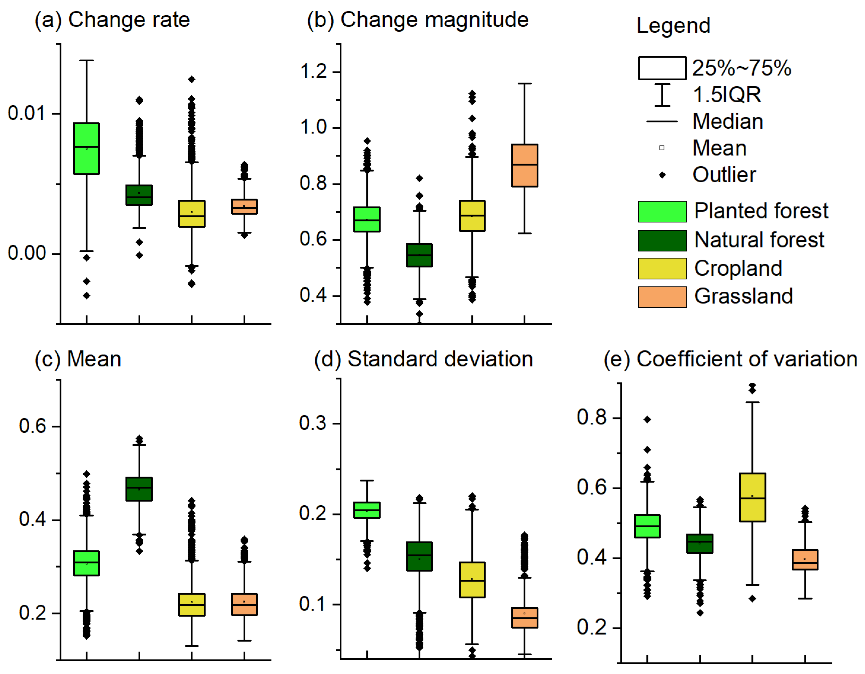
2.2.1. Long-Term Change Trend Features
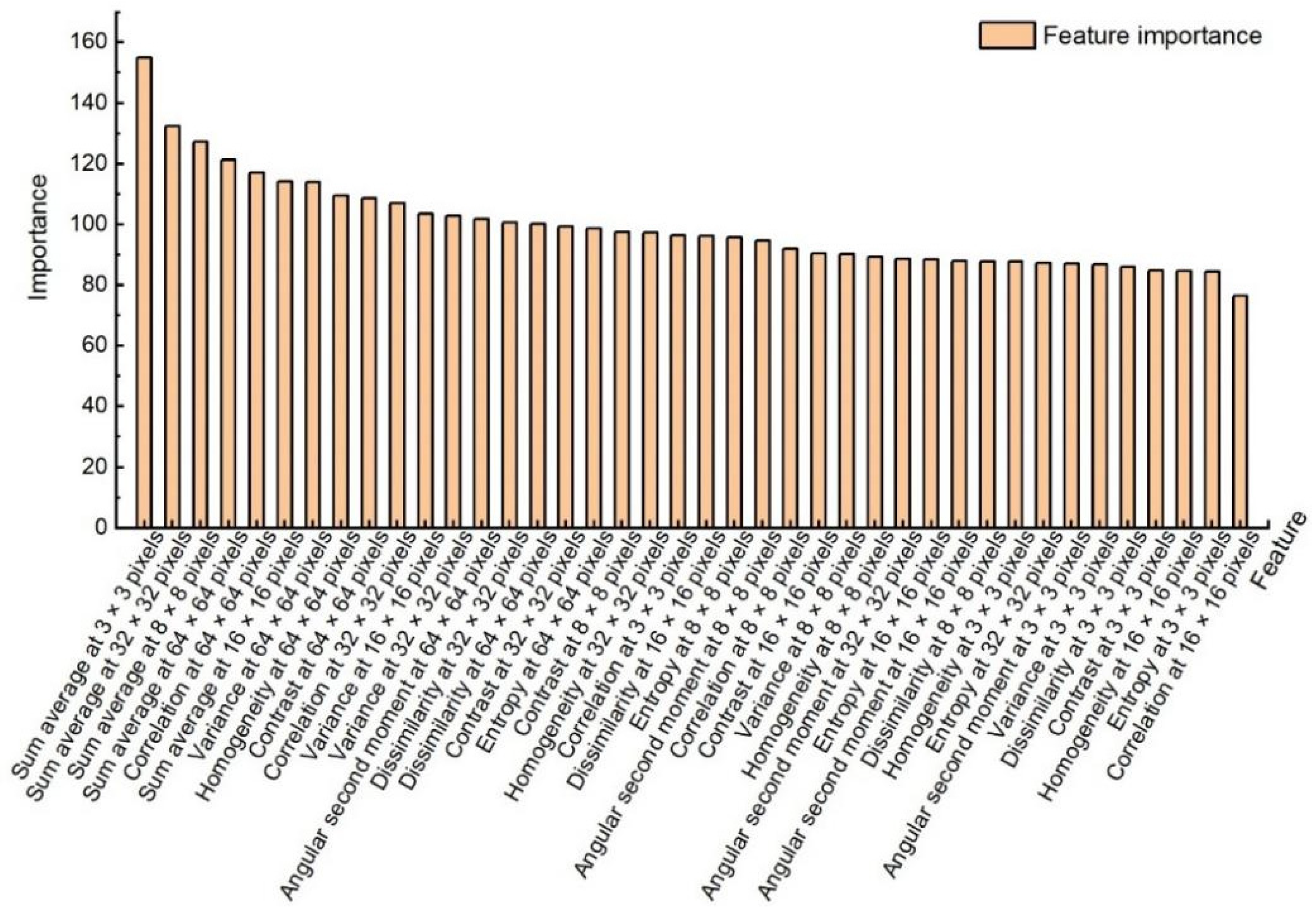
2.2.2. Textural Metrics
2.2.3. Terrain Metrics
2.3. Reference Sample Collection
2.3.1. Field Sampling Data
2.3.2. Reference Data Based on Images
2.4. Classification, Validation and Accuracy Assessment
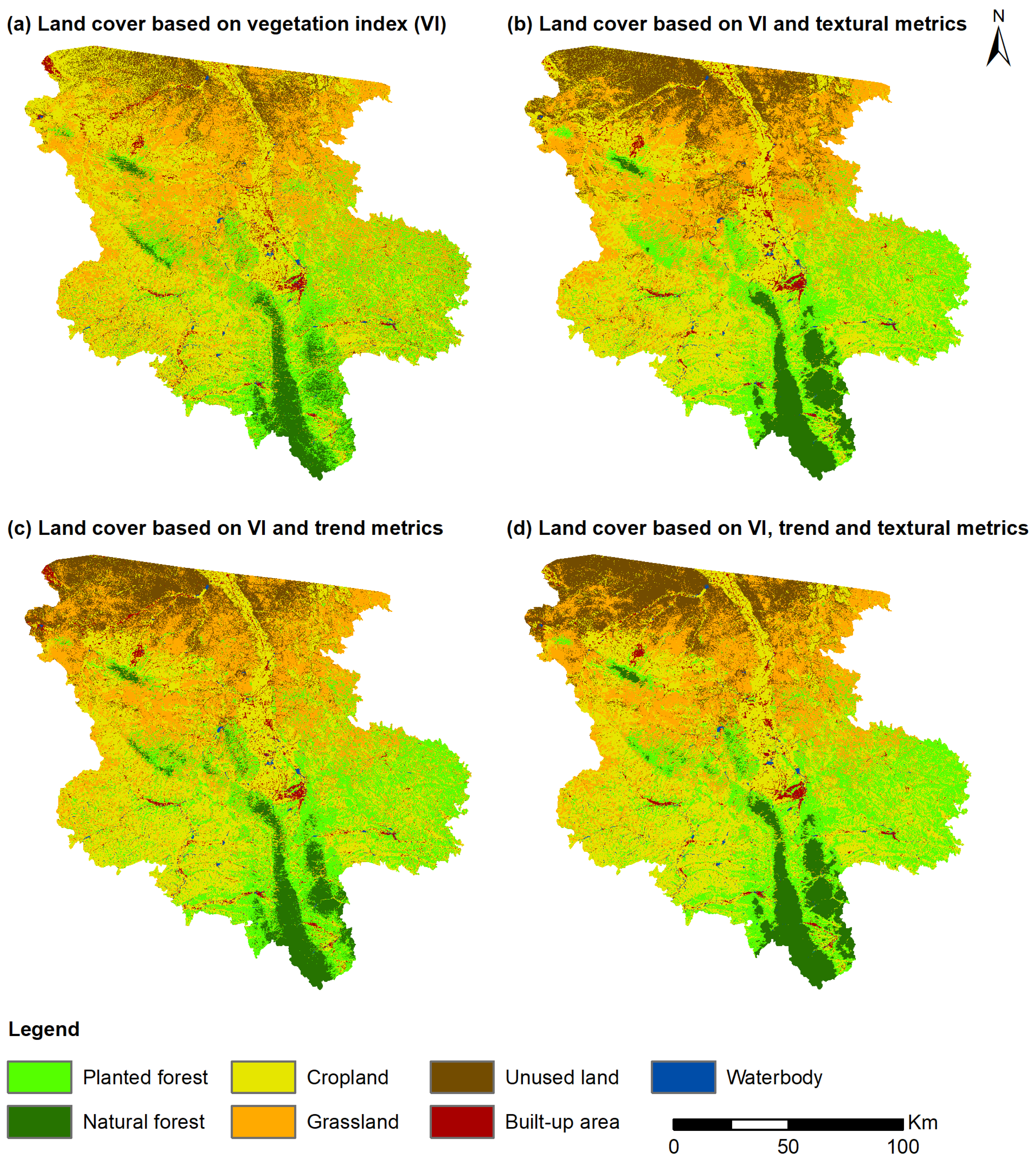
3. Results
4. Discussion
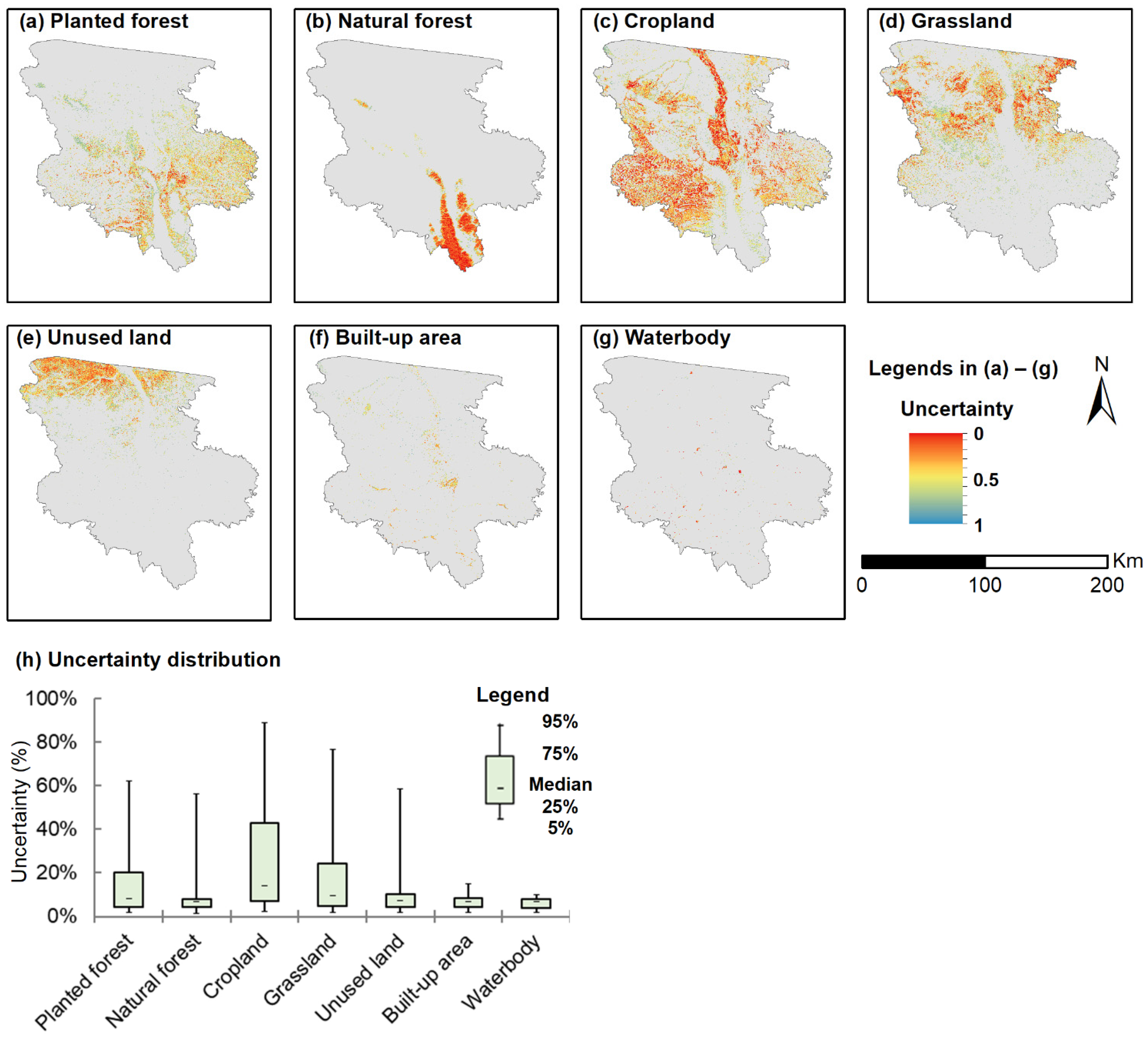
4.1. Uncertainty Analysis
4.2. Limitations and Direction of Future Studies
5. Conclusions
Author Contributions
Funding
Data Availability Statement
Acknowledgments
Conflicts of Interest
Appendix A


| Vegetation Index | Equations | References |
|---|---|---|
| Normalized Difference Vegetation Index (NDVI) | [52] | |
| Enhanced Vegetation Index (EVI) | [53] | |
| Normalized Burn Ratio (NBR) | [54] | |
| Normalized Difference Built-up Index (NDBI) | [55] | |
| Normalized Difference Water Index (NDWI) | [56] | |
| Modified Normalized Difference Water Index (MNDWI) | [57] | |
| Normalized Difference Phenology Index (NDPI) | [58] |
| Texture Features | Equations |
|---|---|
| Angular second moment (ASM) | |
| Contrast (CON) | |
| Correlation (COR) | |
| Variance (VAR) | |
| Homogeneity (HOM) | |
| Sum average (SAVG) | |
| Entropy (ENT) | |
| Dissimilarity (DIS) |
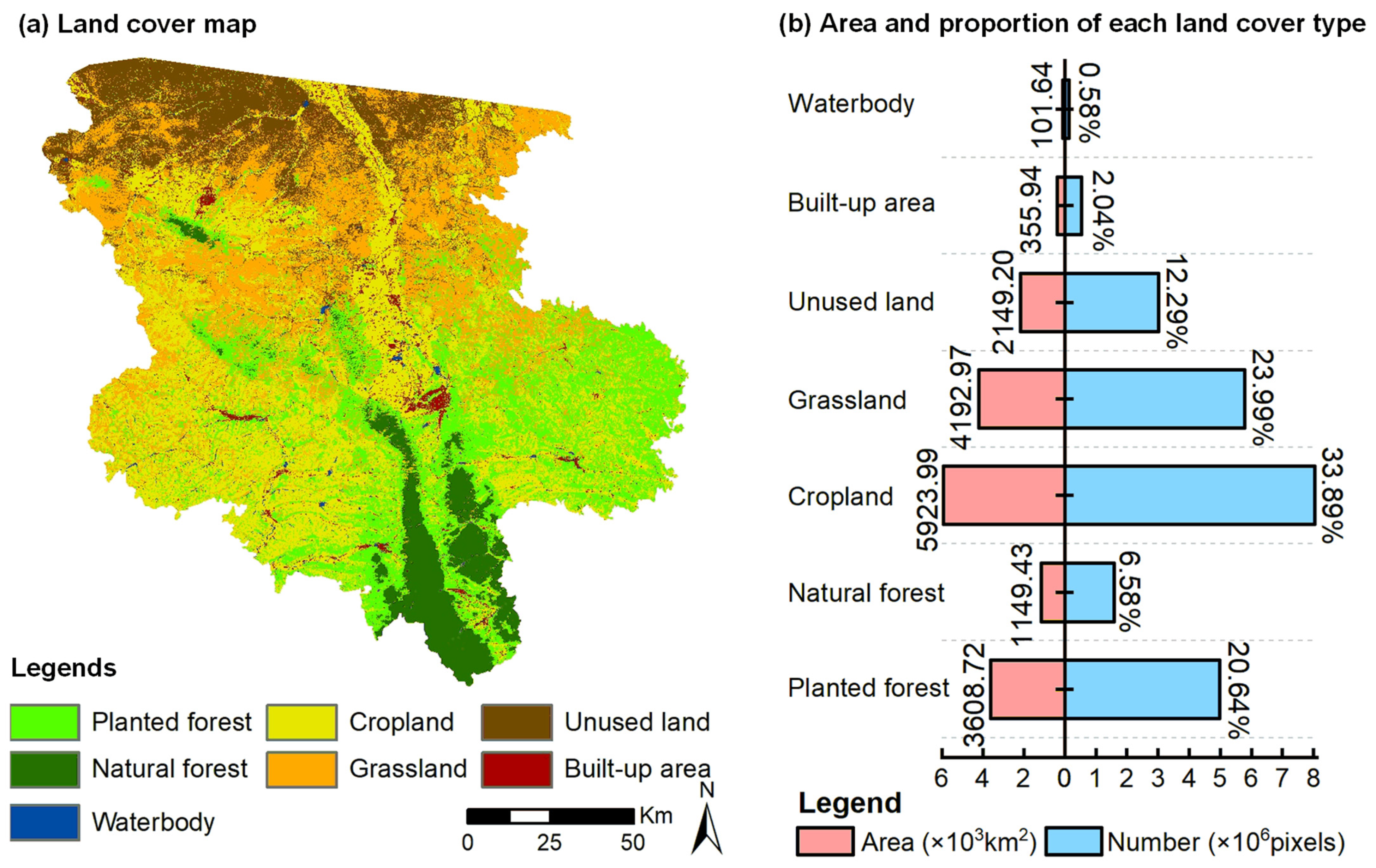
| Land Cover Types | Description |
|---|---|
| Planted forest | Planted trees, shrubs, bamboo and other forest vegetation. |
| Natural forest | Natural trees, shrubs, bamboo and other forest vegetation. |
| Cropland | Land for crop planting, including cultivated land, newly reclaimed land, fallow land, rotation and rest land, and cereal croplands. |
| Grassland | Dominated by herbaceous vegetation. |
| Unused land | Nonvegetated barren (sand, rock, and soil) areas. |
| Built-up area | Land for industrial activities, mining and vehicles in urban and rural residential areas. |
| Waterbody | Covered by permanent water bodies and water conservancy facilities. |
References
- Tong, X.W.; Brandt, M.; Yue, Y.M.; Horion, S.; Wang, K.L.; De Keersmaecker, W.; Tian, F.; Schurgers, G.; Xiao, X.M.; Luo, Y.Q.; et al. Increased vegetation growth and carbon stock in China karst via ecological engineering. Nat. Sustain. 2018, 1, 44–50. [Google Scholar] [CrossRef]
- Wang, Z.; Peng, D.; Xu, D.; Zhang, X.; Zhang, Y. Assessing the water footprint of afforestation in Inner Mongolia, China. J. Arid Environ. 2020, 182, 104257. [Google Scholar] [CrossRef]
- Cao, S.; Chen, L.; Shankman, D.; Wang, C.; Wang, X.; Zhang, H. Excessive reliance on afforestation in China’s arid and semi-arid regions: Lessons in ecological restoration. Earth-Sci. Rev. 2011, 104, 240–245. [Google Scholar] [CrossRef]
- Wang, Y.H.; Brandt, M.; Zhao, M.F.; Tong, X.W.; Xing, K.X.; Xue, F.; Kang, M.Y.; Wang, L.H.; Jiang, Y.; Fensholt, R. Major forest increase on the Loess Plateau, China (2001–2016). Land Degrad. Dev. 2018, 29, 4080–4091. [Google Scholar] [CrossRef]
- Zhang, Y.; Peng, C.H.; Li, W.Z.; Tian, L.X.; Zhu, Q.Q.; Chen, H.; Fang, X.Q.; Zhang, G.L.; Liu, G.M.; Mu, X.M.; et al. Multiple afforestation programs accelerate the greenness in the ‘Three North’ region of China from 1982 to 2013. Ecol. Indic. 2016, 61, 404–412. [Google Scholar] [CrossRef]
- Fassnacht, F.E.; Latifi, H.; Sterenczak, K.; Modzelewska, A.; Lefsky, M.; Waser, L.T.; Straub, C.; Ghosh, A. Review of studies on tree species classification from remotely sensed data. Remote Sens. Environ. 2016, 186, 64–87. [Google Scholar] [CrossRef]
- Griffiths, P.; Kuemmerle, T.; Baumann, M.; Radeloff, V.C.; Abrudan, I.V.; Lieskovsky, J.; Munteanu, C.; Ostapowicz, K.; Hostert, P. Forest disturbances, forest recovery, and changes in forest types across the Carpathian ecoregion from 1985 to 2010 based on Landsat image composites. Remote Sens. Environ. 2014, 151, 72–88. [Google Scholar] [CrossRef]
- Spracklen, B.; Spracklen, D.V. Synergistic Use of Sentinel-1 and Sentinel-2 to map natural forest and acacia plantation and stand ages in North-Central Vietnam. Remote Sens. 2021, 13, 185. [Google Scholar] [CrossRef]
- Tropek, R.; Sedlacek, O.; Beck, J.; Keil, P.; Musilova, Z.; Simova, I.; Storch, D. Comment on “High-resolution global maps of 21st-century forest cover change”. Science 2014, 344, 3. [Google Scholar] [CrossRef] [Green Version]
- Ye, S.; Rogan, J.; Sangermano, F. Monitoring rubber plantation expansion using Landsat data time series and a Shapelet-based approach. Isprs J. Photogramm. Remote Sens. 2018, 136, 134–143. [Google Scholar] [CrossRef]
- Chazdon, R.L.; Brancalion, P.H.S.; Laestadius, L.; Bennett-Curry, A.; Buckingham, K.; Kumar, C.; Moll-Rocek, J.; Vieira, I.C.G.; Wilson, S.J. When is a forest a forest? Forest concepts and definitions in the era of forest and landscape restoration. Ambio 2016, 45, 538–550. [Google Scholar] [CrossRef] [PubMed]
- Xi, W.Q.; Du, S.H.; Du, S.H.; Zhang, X.Y.; Gu, H.Y. Intra-annual land cover mapping and dynamics analysis with dense satellite image time series: A spatiotemporal cube based spatiotemporal contextual method. Giscience Remote Sens. 2021, 58, 1195–1218. [Google Scholar] [CrossRef]
- Ji, Q.; Liang, W.; Fu, B.; Zhang, W.; Yan, J.; Lu, Y.; Yue, C.; Jin, Z.; Lan, Z.; Li, S.Y.; et al. Mapping land use/cover dynamics of the Yellow River Basin from 1986 to 2018 supported by Google Earth Engine. Remote Sens. 2021, 13, 1299. [Google Scholar] [CrossRef]
- Li, Y.C.; Liu, C.L.; Zhang, J.; Zhang, P.; Xue, Y.F. Monitoring spatial and temporal patterns of rubber plantation dynamics using time-series Landsat images and Google Earth Engine. IEEE J. Sel. Top. Appl. Earth Observ. Remote Sens. 2021, 14, 9450–9461. [Google Scholar] [CrossRef]
- Poortinga, A.; Tenneson, K.; Shapiro, A.; Quyen, N.; San Aung, K.; Chishtie, F.; Saah, D. Mapping plantations in Myanmar by fusing Landsat-8, Sentinel-2 and Sentinel-1 data along with systematic error quantification. Remote Sens. 2019, 11, 831. [Google Scholar] [CrossRef] [Green Version]
- Heilmayr, R.; Echeverria, C.; Fuentes, R.; Lambin, E.F. A plantation-dominated forest transition in Chile. Appl. Geogr. 2016, 75, 71–82. [Google Scholar] [CrossRef] [Green Version]
- Gao, T.; Zhu, J.; Zheng, X.; Shang, G.; Huang, L.; Wu, S. Mapping spatial distribution of larch plantations from multi-seasonal Landsat-8 OLI imagery and multi-scale textures using Random Forests. Remote Sens. 2015, 7, 1702–1720. [Google Scholar] [CrossRef] [Green Version]
- Kou, W.; Dong, J.; Xiao, X.; Hernandez, A.J.; Qin, Y.; Zhang, G.; Chen, B.; Lu, N.; Doughty, R. Expansion dynamics of deciduous rubber plantations in Xishuangbanna, China during 2000–2010. Gisci. Remote Sens. 2018, 55, 905–925. [Google Scholar] [CrossRef]
- Torbick, N.; Ledoux, L.; Salas, W.; Zhao, M. Regional mapping of plantation extent using multisensor imagery. Remote Sens. 2016, 8, 236. [Google Scholar] [CrossRef] [Green Version]
- Qiu, B.W.; Zou, F.L.; Chen, C.C.; Tang, Z.H.; Zhong, J.P.; Yan, X.F. Automatic mapping afforestation, cropland reclamation and variations in cropping intensity in central east China during 2001–2016. Ecol. Indic. 2018, 91, 490–502. [Google Scholar] [CrossRef]
- Dong, J.; Xiao, X.; Chen, B.; Torbick, N.; Jin, C.; Zhang, G.; Biradar, C. Mapping deciduous rubber plantations through integration of PALSAR and multi-temporal Landsat imagery. Remote Sens. Environ. 2013, 134, 392–402. [Google Scholar] [CrossRef]
- Bey, A.; Meyfroidt, P. Improved land monitoring to assess large-scale tree plantation expansion and trajectories in Northern Mozambique. Environ. Res. Commun. 2021, 3, 14. [Google Scholar] [CrossRef]
- Fagan, M.E.; Morton, D.C.; Cook, B.D.; Masek, J.; Zhao, F.; Nelson, R.F.; Huang, C. Mapping pine plantations in the southeastern US using structural, spectral, and temporal remote sensing data. Remote Sens. Environ. 2018, 216, 415–426. [Google Scholar] [CrossRef]
- Yu, Z.; Zhao, H.; Liu, S.; Zhou, G.; Fang, J.; Yu, G.; Tang, X.; Wang, W.; Yan, J.; Wang, G.; et al. Mapping forest type and age in China′s plantations. Sci. Total Environ. 2020, 744, 140790. [Google Scholar] [CrossRef] [PubMed]
- Liu, L.Y.; Tang, H.; Caccetta, P.; Lehmann, E.A.; Hu, Y.; Wu, X. Mapping afforestation and deforestation from 1974 to 2012 using Landsat time-series stacks in Yulin District, a key region of the Three-North Shelter region, China. Environ. Monit. Assess. 2013, 185, 9949–9965. [Google Scholar] [CrossRef] [PubMed]
- Wang, F.; Pan, X.; Gerlein-Safdi, C.; Cao, X.; Wang, S.; Gu, L.; Wang, D.; Lu, Q. Vegetation restoration in Northern China: A contrasted picture. Land Degrad. Dev. 2020, 31, 669–676. [Google Scholar] [CrossRef]
- Kim, J.; Song, C.; Lee, S.; Jo, H.; Park, E.; Yu, H.N.; Cha, S.; An, J.; Son, Y.; Khamzina, A.; et al. Identifying potential vegetation establishment areas on the dried Aral Sea floor using satellite images. Land Degrad. Dev. 2020, 31, 2749–2762. [Google Scholar] [CrossRef]
- Li, S.; Yang, S.; Liu, X.; Liu, Y.; Shi, M. NDVI-based analysis on the influence of climate change and human activities on vegetation restoration in the Shaanxi-Gansu-Ningxia Region, Central China. Remote Sens. 2015, 7, 11163–11182. [Google Scholar] [CrossRef] [Green Version]
- Yang, J.; Huang, X. The 30 m annual land cover dataset and its dynamics in China from 1990 to 2019. Earth Syst. Sci. Data 2021, 13, 3907–3925. [Google Scholar] [CrossRef]
- Zhu, Z.; Woodcock, C.E.; Olofsson, P. Continuous monitoring of forest disturbance using all available Landsat imagery. Remote Sens. Environ. 2012, 122, 75–91. [Google Scholar] [CrossRef]
- Roy, D.P.; Kovalskyy, V.; Zhang, H.K.; Vermote, E.F.; Yan, L.; Kumar, S.S.; Egorov, A. Characterization of Landsat-7 to Landsat-8 reflective wavelength and normalized difference vegetation index continuity. Remote Sens. Environ. 2016, 185, 57–70. [Google Scholar] [CrossRef] [PubMed] [Green Version]
- Pan, N.; Feng, X.; Fu, B.; Wang, S.; Ji, F.; Pan, S. Increasing global vegetation browning hidden in overall vegetation greening: Insights from time-varying trends. Remote Sens. Environ. 2018, 214, 59–72. [Google Scholar] [CrossRef]
- Yao, Y.; Piao, S.; Wang, T. Future biomass carbon sequestration capacity of Chinese forests. Sci. Bull. 2018, 63, 1108–1117. [Google Scholar] [CrossRef] [Green Version]
- Wilson, B.T.; Knight, J.F.; McRoberts, R.E. Harmonic regression of Landsat time series for modeling attributes from national forest inventory data. Isprs J. Photogramm. Remote Sens. 2018, 137, 29–46. [Google Scholar] [CrossRef]
- Sellers, P.J.; Tucker, C.J.; Collatz, G.J.; Los, S.O.; Justice, C.O.; Dazlich, D.A.; Randall, D.A. A revised land surface parameterization (SiB2) for atmospheric GCMS. Part II: The generation of global fields of terrestrial biophysical parameters from satellite data. J. Clim. 1996, 9, 706–737. [Google Scholar] [CrossRef] [Green Version]
- Song, D.; Huang, C.; Sexton, J.O.; Channan, S.; Feng, M.; Townshend, J.R. Use of Landsat and Corona data for mapping forest cover change from the mid-1960s to 2000s: Case studies from the Eastern United States and Central Brazil. Isprs J. Photogramm. Remote Sens. 2015, 103, 81–92. [Google Scholar] [CrossRef] [Green Version]
- Tuominen, S.; Pekkarinen, A. Performance of different spectral and textural aerial photograph features in multi-source forest inventory. Remote Sens. Environ. 2005, 94, 256–268. [Google Scholar] [CrossRef]
- Farr, T.G.; Rosen, P.A.; Caro, E.; Crippen, R.; Duren, R.; Hensley, S.; Kobrick, M.; Paller, M.; Rodriguez, E.; Roth, L.; et al. The shuttle radar topography mission. Rev. Geophys. 2007, 45, 33. [Google Scholar] [CrossRef] [Green Version]
- Olofsson, P.; Foody, G.M.; Herold, M.; Stehman, S.V.; Woodcock, C.E.; Wulder, M.A. Good practices for estimating area and assessing accuracy of land change. Remote Sens. Environ. 2014, 148, 42–57. [Google Scholar] [CrossRef]
- Cao, B.; Yu, L.; Naipal, V.; Ciais, P.; Li, W.; Zhao, Y.; Wei, W.; Chen, D.; Liu, Z.; Gong, P. A 30-meter terrace mapping in China using Landsat 8 imagery and digital elevation model based on the Google Earth Engine. Earth Syst. Sci. Data 2021, 13, 2437–2456. [Google Scholar] [CrossRef]
- Loosvelt, L.; Peters, J.; Skriver, H.; Lievens, H.; Van Coillie, F.M.B.; De Baets, B.; Verhoest, N.E.C. Random Forests as a tool for estimating uncertainty at pixel-level in SAR image classification. Int. J. Appl. Earth Obs. Geoinf. 2012, 19, 173–184. [Google Scholar] [CrossRef]
- Zhu, Z.; Fu, Y.C.; Woodcock, C.E.; Olofsson, P.; Vogelmann, J.E.; Holden, C.; Wang, M.; Dai, S.; Yu, Y. Including land cover change in analysis of greenness trends using all available Landsat 5, 7, and 8 images: A case study from Guangzhou, China (2000–2014). Remote Sens. Environ. 2016, 185, 243–257. [Google Scholar] [CrossRef] [Green Version]
- Zhu, Z.; Woodcock, C.E.; Holden, C.; Yang, Z.Q. Generating synthetic Landsat images based on all available Landsat data: Predicting Landsat surface reflectance at any given time. Remote Sens. Environ. 2015, 162, 67–83. [Google Scholar] [CrossRef]
- Vogeler, J.C.; Braaten, J.D.; Slesak, R.A.; Falkowski, M.J. Extracting the full value of the Landsat archive: Inter-sensor harmonization for the mapping of Minnesota forest canopy cover (1973–2015). Remote Sens. Environ. 2018, 209, 363–374. [Google Scholar] [CrossRef]
- Amani, M.; Brisco, B.; Afshar, M.; Mirmazloumi, S.M.; Mahdavi, S.; Mirzadeh, S.M.; Huang, W.; Granger, J. A generalized supervised classification scheme to produce provincial wetland inventory maps: An application of Google Earth Engine for big geo data processing. Big Earth Data 2019, 3, 378–394. [Google Scholar] [CrossRef]
- Hu, J.; Xia, G.S.; Hu, F.; Zhang, L.P. A comparative study of sampling analysis in the scene classification of optical high-spatial resolution remote sensing imagery. Remote Sens. 2015, 7, 14988–15013. [Google Scholar] [CrossRef] [Green Version]
- Tong, X.Y.; Xia, G.S.; Lu, Q.K.; Shen, H.F.; Li, S.Y.; You, S.C.; Zhang, L.P. Land-cover classification with high-resolution remote sensing images using transferable deep models. Remote Sens. Environ. 2020, 237, 20. [Google Scholar] [CrossRef] [Green Version]
- Ghorbanian, A.; Kakooei, M.; Amani, M.; Mahdavi, S.; Mohammadzadeh, A.; Hasanlou, M. Improved land cover map of Iran using Sentinel imagery within Google Earth Engine and a novel automatic workflow for land cover classification using migrated training samples. ISPRS J. Photogramm. Remote Sens. 2020, 167, 276–288. [Google Scholar] [CrossRef]
- Chen, Y.; Wang, K.; Lin, Y.; Shi, W.; Song, Y.; He, X. Balancing green and grain trade. Nat. Geosci. 2015, 8, 739–741. [Google Scholar] [CrossRef]
- Chen, P.; Shang, J.; Qian, B.; Jing, Q.; Liu, J. A new regionalization scheme for effective ecological restoration on the Loess Plateau in China. Remote Sens. 2017, 9, 1323. [Google Scholar] [CrossRef] [Green Version]
- Gelviz-Gelvez, S.M.; Pavon, N.P.; Illoldi-Rangel, P.; Ballesteros-Barrera, C. Ecological niche modeling under climate change to select shrubs for ecological restoration in Central Mexico. Ecol. Eng. 2015, 74, 302–309. [Google Scholar] [CrossRef]
- Tucker, C.J. Red and photographic infrared linear combinations for monitoring vegetation. Remote Sens. Environ. 1979, 8, 127–150. [Google Scholar] [CrossRef] [Green Version]
- Huete, A.; Didan, K.; Miura, T.; Rodriguez, E.P.; Gao, X.; Ferreira, L.G. Overview of the radiometric and biophysical performance of the MODIS vegetation indices. Remote Sens. Environ. 2002, 83, 195–213. [Google Scholar] [CrossRef]
- Key, C.H.; Benson, N.C. Landscape assessment: Sampling and analysis methods. In General Technical Report RMRS-GTR-164-CD; USDA Forest Service, Rocky Mountain Research Station: Fort Collins, CO, USA, 2006; pp. 1–55. [Google Scholar]
- Zha, Y.; Gao, J.; Ni, S. Use of normalized difference built-up index in automatically mapping urban areas from TM imagery. Int. J. Remote Sens. 2003, 24, 583–594. [Google Scholar] [CrossRef]
- McFeeters, S.K. The use of the normalized difference water index (NDWI) in the delineation of open water features. Int. J. Remote Sens. 1996, 17, 1425–1432. [Google Scholar] [CrossRef]
- Xu, H.Q. Modification of normalised difference water index (NDWI) to enhance open water features in remotely sensed imagery. Int. J. Remote Sens. 2006, 27, 3025–3033. [Google Scholar] [CrossRef]
- Wang, C.; Chen, J.; Wu, J.; Tang, Y.H.; Shi, P.J.; Black, T.A.; Zhu, K. A snow-free vegetation index for improved monitoring of vegetation spring green-up date in deciduous ecosystems. Remote Sens. Environ. 2017, 196, 1–12. [Google Scholar] [CrossRef]


| Land Cover Types | Field Survey Data | 7th National Forest Inventory | Image Data | Total Number |
|---|---|---|---|---|
| Planted forest | 695 | 0 | 0 | 695 |
| Natural forest | 120 | 135 | 0 | 255 |
| Cropland | 0 | 0 | 1406 | 1406 |
| Grassland | 0 | 0 | 722 | 722 |
| Unused land | 0 | 0 | 438 | 438 |
| Built-up area | 0 | 0 | 520 | 520 |
| Waterbody | 0 | 0 | 464 | 464 |
| Total number | 815 | 135 | 3550 | 4500 |
| Land Cover Types | Planted Forest | Natural Forest | Crop-Land | Grass-Land | Unused Land | Built-Up Area | Water-Body | Total | PA |
|---|---|---|---|---|---|---|---|---|---|
| Using the vegetation index (VI) | |||||||||
| Planted forest | 100 | 4 | 7 | 17 | 1 | 0 | 1 | 130 | 76.92% |
| Natural forest | 16 | 37 | 0 | 0 | 0 | 0 | 0 | 53 | 69.81% |
| Cropland | 4 | 0 | 242 | 10 | 2 | 6 | 0 | 264 | 91.67% |
| Grassland | 10 | 1 | 2 | 112 | 6 | 0 | 0 | 131 | 85.50% |
| Unused land | 0 | 0 | 8 | 3 | 68 | 1 | 0 | 80 | 85.00% |
| Built-up area | 0 | 0 | 21 | 0 | 1 | 94 | 0 | 116 | 81.03% |
| Waterbody | 1 | 0 | 3 | 0 | 2 | 1 | 93 | 100 | 93.00% |
| Total | 131 | 42 | 283 | 142 | 80 | 102 | 94 | OA 85.35% Kappa 0.82 | |
| UA | 76.34% | 88.10% | 85.51% | 78.87% | 85.00% | 92.16% | 98.94% | ||
| Using VI and GLCM-based textural metrics | |||||||||
| Plantedforest | 105 | 3 | 8 | 9 | 3 | 0 | 1 | 129 | 81.40% |
| Naturalforest | 10 | 37 | 1 | 3 | 0 | 0 | 0 | 51 | 72.55% |
| Cropland | 8 | 2 | 252 | 5 | 6 | 6 | 0 | 279 | 90.32% |
| Grassland | 8 | 2 | 3 | 131 | 3 | 0 | 0 | 147 | 89.12% |
| Unused land | 0 | 0 | 5 | 8 | 72 | 1 | 0 | 86 | 83.72% |
| Built-up area | 0 | 0 | 10 | 1 | 1 | 106 | 5 | 123 | 86.18% |
| Waterbody | 3 | 0 | 5 | 0 | 0 | 0 | 79 | 87 | 90.80% |
| Total | 134 | 44 | 284 | 157 | 85 | 113 | 85 | OA 85.73% Kappa 0.83 | |
| UA | 78.36% | 84.09% | 88.73% | 83.44% | 84.71% | 93.81% | 92.94% | ||
| Using VI and long-term change trend metrics | |||||||||
| Planted forest | 116 | 4 | 7 | 7 | 0 | 0 | 0 | 134 | 86.57% |
| Natural forest | 0 | 42 | 0 | 0 | 0 | 0 | 0 | 42 | 100.00% |
| Cropland | 8 | 0 | 268 | 0 | 2 | 3 | 0 | 281 | 95.37% |
| Grassland | 1 | 0 | 2 | 132 | 1 | 0 | 0 | 136 | 97.06% |
| Unused land | 0 | 0 | 2 | 7 | 79 | 4 | 0 | 92 | 85.87% |
| Built-up area | 0 | 0 | 3 | 0 | 0 | 97 | 4 | 104 | 93.27% |
| Waterbody | 0 | 0 | 3 | 0 | 0 | 3 | 94 | 100 | 94.00% |
| Total | 125 | 46 | 285 | 146 | 82 | 107 | 98 | OA 93.14% Kappa 0.91 | |
| UA | 92.80% | 91.30% | 94.04% | 90.41% | 96.34% | 90.65% | 95.92% | ||
| Using VI, textural metrics, and long-term change trend metrics | |||||||||
| Planted forest | 123 | 1 | 4 | 4 | 0 | 1 | 0 | 133 | 92.48% |
| Natural forest | 3 | 46 | 0 | 0 | 0 | 0 | 0 | 49 | 93.88% |
| Cropland | 5 | 0 | 259 | 0 | 2 | 3 | 0 | 269 | 96.28% |
| Grassland | 2 | 1 | 2 | 143 | 5 | 0 | 0 | 153 | 93.46% |
| Unused land | 1 | 0 | 3 | 5 | 75 | 3 | 0 | 87 | 86.21% |
| Built-up area | 0 | 0 | 4 | 0 | 1 | 109 | 2 | 116 | 93.97% |
| Waterbody | 0 | 0 | 2 | 0 | 1 | 2 | 85 | 90 | 94.44% |
| Total | 134 | 48 | 274 | 152 | 84 | 118 | 87 | OA 93.65% Kappa 0.92 | |
| UA | 91.79% | 95.83% | 94.53% | 94.08% | 89.29% | 92.37% | 97.70% | ||
Publisher’s Note: MDPI stays neutral with regard to jurisdictional claims in published maps and institutional affiliations. |
© 2022 by the authors. Licensee MDPI, Basel, Switzerland. This article is an open access article distributed under the terms and conditions of the Creative Commons Attribution (CC BY) license (https://creativecommons.org/licenses/by/4.0/).
Share and Cite
Meng, Y.; Wei, C.; Guo, Y.; Tang, Z. A Planted Forest Mapping Method Based on Long-Term Change Trend Features Derived from Dense Landsat Time Series in an Ecological Restoration Region. Remote Sens. 2022, 14, 961. https://doi.org/10.3390/rs14040961
Meng Y, Wei C, Guo Y, Tang Z. A Planted Forest Mapping Method Based on Long-Term Change Trend Features Derived from Dense Landsat Time Series in an Ecological Restoration Region. Remote Sensing. 2022; 14(4):961. https://doi.org/10.3390/rs14040961
Chicago/Turabian StyleMeng, Yuanyuan, Caiyong Wei, Yanpei Guo, and Zhiyao Tang. 2022. "A Planted Forest Mapping Method Based on Long-Term Change Trend Features Derived from Dense Landsat Time Series in an Ecological Restoration Region" Remote Sensing 14, no. 4: 961. https://doi.org/10.3390/rs14040961