Article

Assessing the Impact of Soil on Species Diversity Estimation Based on UAV Imaging Spectroscopy in a Natural Alpine Steppe

1
State Key Laboratory of Remote Sensing Science, Aerospace Information Research Institute, Chinese Academy of Sciences, Beijing 100101, China
2
University of Chinese Academy of Sciences, Beijing 100049, China
3
Remote Sensing Laboratories, Department of Geography, University of Zurich, CH-8057 Zurich, Switzerland
4
School of Ecology and Environmental Science, Yunnan University, Kunming 650091, China
*
Author to whom correspondence should be addressed.
Remote Sens. 2022, 14(3), 671; https://doi.org/10.3390/rs14030671
Submission received: 22 December 2021 / Revised: 22 January 2022 / Accepted: 29 January 2022 / Published: 30 January 2022
(This article belongs to the Special Issue Remote Sensing of Ecosystems)

Abstract

:
Grassland species diversity monitoring is essential to grassland resource protection and utilization. “Spectral variation hypothesis” (SVH) provides a remote sensing method for monitoring grassland species diversity at pixel scale by calculating spectral heterogeneity. However, the pixel spectrum is easily affected by soil and other background factors in natural grassland. Unmanned aerial vehicle (UAV)-based imaging spectroscopy provides the possibility of soil information removal by virtue of its high spatial and spectral resolution. In this study, UAV-imaging spectroscopy data with a spatial resolution of 0.2 m obtained in two sites of typical alpine steppe within the Sanjiangyuan National Nature Reserve were used to analyze the relationships between four spectral diversity metrics (coefficient of variation based on NDVI (CVNDVI), coefficient of variation based on multiple bands (CVMulti), minimum convex hull volume (CHV) and minimum convex hull area (CHA)) and two species diversity indices (species richness and the Shannon–Wiener index). Meanwhile, two soil removal methods (based on NDVI threshold and the linear spectral unmixing model) were used to investigate the impact of soil on species diversity estimation. The results showed that the Shannon–Wiener index had a better response to spectral diversity than species richness, and CVMulti showed the best correlation with the Shannon–Wiener index between the four spectral diversity metrics after removing soil information using the linear spectral unmixing model. It indicated that the estimation ability of spectral diversity to species diversity was significantly improved after removing the soil information. Our findings demonstrated the applicability of the spectral variation hypothesis in natural grassland, and illustrated the impact of soil on species diversity estimation.

1. Introduction

Grassland biodiversity is critical for the long-term restoration and support services of ecosystem functions [1,2,3], and is directly related to human society [4,5]. However, biodiversity is being lost due to climate change and human activities, and this trend is likely to continue in the future [6,7]. Grasslands bear the brunt of biodiversity loss due to ecosystem vulnerability and severe environmental pressure [8,9]. The Aichi target set in response to the continuing loss of global biodiversity has not yet been fully achieved [10]. The biodiversity of grassland can be divided into three levels: genetic diversity, species diversity and ecosystem diversity [11]. As the primary component of biodiversity, the species diversity of grassland remains a top priority in biodiversity monitoring.
Species diversity refers to biodiversity at the species level and can be considered at least from taxonomic, functional, and phylogenetic diversity perspectives [12,13,14]. In terms of taxonomic diversity, there are three measures based on scale dependence: α-diversity focuses on the composition of species and distribution of each species within a community, while β-diversity and γ-diversity represent the differences and synthesis between communities, respectively [15,16,17]. α-diversity, or within-habitat diversity, is most commonly used in regional species diversity monitoring and is usually demonstrated by four indicators, including species richness [16,18], Shannon–Weiner index [19,20], Simpson index [21,22] and Pielou evenness [23]. Among these, species richness is the number of different species, for which it is easier to obtain an accurate value by ground sampling. The Shannon–Wiener index and Simpson index have certain similarities, because both indices take species uniformity into account. In addition, towards the grassland diversity estimation, species richness and the Shannon–Wiener index are the more generally used indicators in the ecological and remote-sensing literature. For example, Tilman et al. [24] proved the diversity–stability hypothesis based on the variation of species richness during a decade of data collection at Cedar Creek Natural History Area. Jochum et al. [25] used species richness and the Shannon–Wiener index as indicators of taxonomic diversity to verify that the results of biodiversity-ecosystem functioning experiments were realistic in the real world.
A grassland species diversity survey is generally based on field measurements, which usually obtain accurate information for small areas. However, it is time-consuming and labor-intensive to cover large regions, and field data are prone to inconsistencies [26,27]. Remote sensing can provide spatiotemporal continuous data and assess species diversity loss of all scales in a repeatable and rapid manner [28,29,30], which has been recognized as an efficient tool in the global monitoring of biodiversity [31,32,33,34]. The technological advances in airborne and UAV-based imaging spectrometers, which measure continuous spectral coverage with high spatial resolution, provide great potential in monitoring grassland biodiversity efficiently across large areas [32,35,36].
Monitoring species diversity by remote sensing can be divided into roughly two categories: identifying the species directly and estimating the spatial distribution of species diversity indirectly based on habitat or relevant indicators [29,37]. Compared with direct species identification methods limited to big-size species or nonmixed species, spectral variation hypothesis (SVH), as the most representative indirect observation method, has strong applicability in monitoring species diversity [38,39,40,41]. The spectral variation hypothesis [38] assumes that the remotely sensed variation in spectral patterns is related to plant species diversity. There were many SVH-based applications at the individual canopy level of the forest, especially in combination with light detection and ranging (LiDAR) data, both in terms of species and functional diversity estimation [42,43,44,45]. However, the main challenge for monitoring grassland species diversity by remote sensing is the small size of plants, structural heterogeneity, and highly mixed species. The complex canopy structure of grassland makes it difficult to estimate species diversity at individual grass scale [46,47,48,49]. Therefore, spectral diversity was proposed for grassland species diversity estimation at pixel scale [32,41,50,51,52].
Spectral diversity refers to the heterogeneity of the vegetation spectrum caused by some characteristics of species, including physiological and biochemical components, phenological characteristics and canopy structure [41,49]. Many spectral diversity metrics, such as coefficient of variation (CV) [53], convex hull volume (CHV) or area (CHA) [32,51,52], spectral angle mapper (SAM) [54], and distance from the spectral centroid [55], have been developed to monitor grassland species diversity. All the metrics are based on the principle of condensing multidimensional spectral information of vegetation into a statistical measure [49]. However, whether spectral diversity works for estimating grassland species diversity, depends on several factors, such as spectral resolution and band selection, the chosen spectral diversity metrics and background disturbances such as soil, dead materials and shadows [36,56,57].
Calculating spectral diversity metrics may use a single band or characteristic vegetation index (VI) or multiple spectral bands. For instance, Gould et al. [58] estimated vascular species richness based on variation in NDVI in the Hood River region. Gholizadeh et al. [32] used averaged CV of 142 bands (427–914 nm) as a proxy of α-diversity to estimate grassland species diversity within the Central Platte River ecosystem. VIs can be obtained from commonly-used satellite remote-sensing data and applied to monitor grassland species diversity over a large geographical extent [55,59]. In contrast, spectral diversity metrics based on multiple spectral bands take advantage of increased spectral information, but may also produce the problem of data redundancy [37,60]. In addition, it should be noted that spectral diversity metrics are vulnerable to interference from the soil information of pixels, which will significantly increase the local spectral heterogeneity, thus leading to species diversity estimation with higher values [37,52]. Even spectral diversity showed a negative correlation with species diversity under the influence of soil, which is contrary to the general knowledge [61].
One commonly used method for removing soil information is to set a threshold of NDVI, such as Gholizadeh et al. [52], who selected pixels with an NDVI larger than 0.4 as vegetation based on proximal imaging spectrometry data with 0.001 m spatial resolution, while Zhao et al. [62] applied a threshold of 0.2 to UAV-imaging spectrometry data with 0.03 m spatial resolution. The spectral unmixing model is another method used for soil removal, for example, Gholizadeh et al. [52] extracted vegetation information by the fully constrained least squares spectral unmixing approach based on UAV-imaging spectroscopy data with 0.75 m spatial resolution. Setting NDVI thresholds is relatively simple, but the thresholds are not consistent and can result in a loss of nonsoil information by removing the entire pixel. The spectral unmixing model may keep the vegetation information at pixel scale, but the acquisition of the pure spectra of vegetation and soil in the image is difficult [63]. Meanwhile, regardless of the methods, soil removal is also related to the spatial resolution of observation.
Therefore, the objective of our study is to investigate the optimal spectral metrics to monitor the species diversity of natural alpine grassland while considering the impact of soil background. We compared two species-diversity indices, four spectral-diversity metrics and two approaches of soil removal by using UAV imaging spectroscopy with 0.2 m spatial resolution. The results may provide a reference for the selection of parameters in monitoring grassland species diversity by remote sensing under natural conditions.

2. Materials and Methods
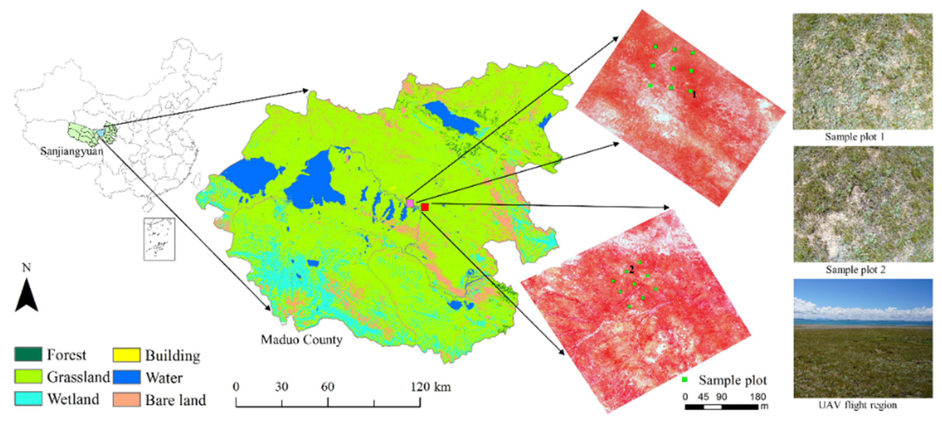
2.1. Study Area

This study area includes two UAV flight regions (center coordinates: 34°49′12″N, 98°25′12″E and 34°50′14″N, 98°19′23″E) in Maduo county at the Sanjiangyuan National Nature Reserve, Qinghai Province of China (Figure 1). Sanjiangyuan National Nature Reserve is one of the most biodiverse areas in the world and there are 760 species of vascular plants belonging to 241 genera and 50 families [64]. The average annual temperature is about −4℃ and the average annual precipitation is 303.9 mm, based on the meteorological records of the monthly standard weather station dataset (1957–2015) [65]. Maduo county, being the source of the Yellow River, is a high plain (altitude > 4000 m) with 80% acreage of grassland and has been regarded as a key conservation area for grassland diversity. Surveys show that this county is characterized by alpine meadow and alpine steppe, the dominant species are Elymus dahuricus, Leontopodium leontopodioides, Kobresia myosuroides, Potentilla chinensis, Oxytropis ochrocephala, etc. [66]. We set two UAV flight regions (No.1: 400 m × 300 m; No.2: 400 m × 400 m) with natural alpine steppe in Maduo county, where complex species composition (more than 20 dominant species) ensured the heterogeneity gradient of sample plots.

2.2. Imaging Spectroscopy Data and Preprocessing

The imaging spectroscopy data were collected on 20 August 2018 from 11:00 to 14:00 local time under cloudless conditions in Maduo county using the M600 UAV platform (DJI, Shenzhen, China). The grassland was in the growing season, which avoided spectral heterogeneity caused by the death of species. We used the UAV platform with a ZK-VNIR-FPG480 push-broom hyperspectral sensor (ZKYD Data Technology Co., Ltd., Beijing, China), which provided a spectral range of 390–1020 nm with 2.3 nm spectral resolution and a total of 270 spectral channels. We set the spatial resolution of the imaging spectroscopy data and flight altitude as 0.2 m and 150 m, respectively. Therefore, detailed ground information could be obtained, and the errors of ground sample distance caused by high flight altitude could be minimized.
The preprocessing of imaging spectroscopy data consisted of three preliminary steps. Spectral radiation calibration was performed as the first step to determine the central wavelength and bandwidth of each band, as well as the corresponding relationship between the spectral response and the true spectral radiance. Then, the reflectivity spectrum of grass was calculated based on the spectral radiance and the reference spectrum of the reflectivity whiteboard. The hyperspectral reflectance data containing geographic coordinate information was finally obtained after geometric correction based on ground control points and the curved surface spline function [68].

2.3. Field Measurements

The field measurements were conducted simultaneously with UAV-hyperspectral image acquisition. We regularly set 9 sample plots (1 m × 1 m) in both flight regions following a criterion that most dominant species within the flight regions should be included. The central coordinate pairs of each plot were recorded through a Trimble GeoXH 3000 handheld GPS and differential correction was done based on a differentially corrected global positioning system to minimize errors. The detailed survey for each sample plot included grassland species, individual coverage and number of each species. A total of 18 sample plots and 22 grassland species were investigated and there was a gradient from 3 to 8 in the number of species for each sample plot. Since the height of most species in the flight regions was about 5–10 cm, there was no significant vertical structure. The shadows or species overlap would not interfere with the calculation of spectral diversity metrics.

2.4. Species Diversity Indices

We used species richness and Shannon–Wiener index to represent species diversity and calculated them within each sample plot of 1 m2. Species richness refers to the total number of different grassland species. Shannon–Wiener index (H′) consists of two components: species number and equitability or evenness of species distribution [23,59,69]. The Shannon–Wiener index was calculated based on the following formula:
  H = i = 1 n p i ln ( p i )
where n is the total number of different species in a sample plot; pi is the proportional abundance of the species i; ln(pi) is the natural logarithm of this proportion.
Shannon–Wiener index gradually increases to the maximum value from zero, as the species distribution within the plot changes from only one species to the same abundance of all different species [70].

2.5. Spectral Diversity Metrics

CV, CHA and CHV were selected as the spectral diversity metrics in our study after comprehensively analyzing the principle and applicability of several frequently used metrics. Among them, CV could be calculated by both characteristic vegetation index (CVNDVI) and multibands (CVMulti), but CHA and CHV were necessarily based on multibands. It should be noted that all spectral diversity metrics were calculated within a pixel set of 5 × 5 in order to match the 1 m × 1 m ground sample plot.
CVNDVI was calculated based on the mean and standard deviation of NDVI (Equation (2)) of all the pixels within a sample plot (Equation (3)), while CVMulti was the mean of coefficients of variation for all bands from 390 nm to 1020 nm (Equation (4)).
NDVI = ρ 860 ρ 660 ρ 860 + ρ 660
CV NDVI = std ( NDVI ) mean ( NDVI )
CV Multi = λ = 390 1020 ( std ( ρ λ ) mean ( ρ λ ) ) n
where NDVI was calculated based on central reflectance of near-infrared (860 nm) and red (660 nm); std (NDVI) and mean (NDVI) are the standard deviation and mean value of NDVI of all pixels in a ground sample plot, while std (ρλ) and mean (ρλ) are standard deviation and mean value of reflectance at band λ; ρλ is the reflectance of band λ; n is the number of bands, which was 270 in our study.
CHV is another metric of spectral diversity, which represents the minimum volume of the convex hull formed by three-dimensional spectral information. The three-dimensional spectral information is usually obtained by dimensionality reduction of n-dimensional imaging spectroscopy data. The first three dimensions of principal component analysis (PCA) could explain 85–90% of the total information according to the gravel figure, so we used the first three principal components of the reflectance values to calculate CHV (convhull, matlab) in our study.
CHA represents the minimum area of the convex hull in a two-dimensional space formed by both the reflectance of each pixel and the mean reflectance of all pixels in one sample plot [52]. It maximizes the spectral separation between the sample plot and each pixel within this sample plot. The average value of CHA of all effective pixels represents the CHA of the sample plot, which was calculated as follows:
CHA L ¯ = K = 1 m CHA ( R K , L , R L ¯ ) m
where CHA L ¯ is the spectral diversity of a sample plot; m is the number of effective pixels of Lth plot; R K , L and R L ¯ , respectively, define two dimensions of the convex hull and R K , L represents the Kth pixel in Lth plot, while R L ¯ is the mean spectrum of all pixels in Lth plot and both are n × 1 vectors where n is band number; CHA ( R K , L , R L ¯ ) represents the area between Kth pixel and the average of Lth plot and it nears to 0 when the spectra of one pixel is extremely similar to the average spectra of sample plot.

2.6. Soil Filtering

We respectively applied two methods to filter soil information. One is setting NDVI thresholds. In this study, we used three thresholds of NDVI (0.2, 0.3 and 0.4) based on the previous studies [52,62]. Pixels with NDVI below the thresholds were removed and the four spectral diversity metrics (i.e., CVNDVI, CVMulti, CHA and CHV) of each sample plot were recalculated using the remaining pixels.
Another method is using the spectral unmixing model, which decomposes the mixed pixel into different basic components (i.e., endmembers) to filter soil information. In general, the linear spectral unmixing model considers the spectra of the mixed pixels as the linear addition of the spectra of vegetation and soil according to their respective proportions (Equations (6) and (7)).
For the pure soil selection, we marked three bare soil ground samples (0.5 m × 0.5 m) in each flight region and collected the spectra of bare soil by ASD field spectroradiometers (ASD Co., Alpharetta, GA, USA). Then we selected a total of 54 pixels from the UAV-hyperspectral imagery that were similar to the field spectra of bare soil and calculated their average spectrum as the pure soil spectrum for spectral unmixing model. Meanwhile, the fractions for both vegetation and soil were obtained from the FVC (fractional vegetation coverage) products based on dimidiate pixel mode [71,72]. Therefore, the pure vegetation spectrum of each pixel could be extracted by inverting the linear spectral unmixing model [73].
R j = R veg , j   F veg + R soil , j   F soil   j = 1 , 2 , , p
1 = F veg + F soil   F veg ,   F soil 0
where R j is the reflectance of the mixed pixel in band j; R veg , j is the pure reflectance for vegetation components in band j and R soil , j is the pure reflectance of soil components in band j; F veg and F soil are the fractional coverage of vegetation and soil within the pixel and their sum is equal to 1.

3. Results

The performance of the relationships between the two species diversity indices and the four spectral diversity metrics before and after removing the soil based on two different methods are listed as follows (Table 1).

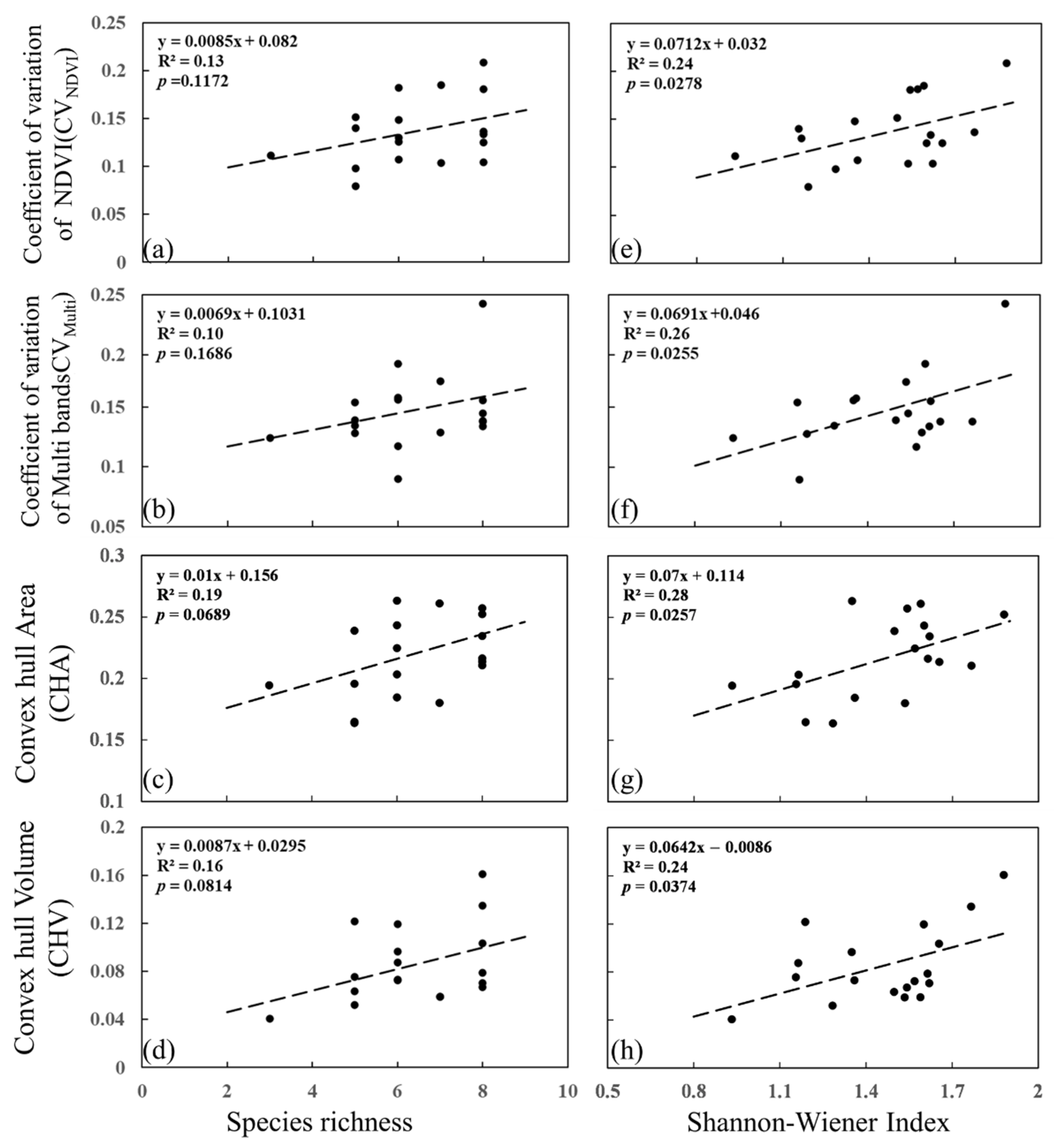
3.1. Responses of Spectral Diversity to Species Diversity

The correlations between four spectral diversity metrics (CVNDVI, CVMulti, CHV and CHA) and two species diversity indices (species richness and Shannon–Wiener index) are shown in Figure 2. From the perspective of species diversity indices, Shannon–Wiener index showed a significant positive correlation with all spectral diversity metrics (p < 0.05) compared to species richness. Species richness just reveals how many species exist in a certain region and cannot reflect the uniformity of the distribution of species, but the uniformity can be indicated by Shannon–Wiener index based on the species richness and their relative abundance (evenness). Therefore, the Shannon–Wiener index could better respond to the spectral diversity, which is consistent with the previous study of Oldeland [70]. Moreover, Figure 2a–d show the variation of spectral diversity with the same species richness. For example, the differences between the maximum and minimum CVMulti were 0.10 with six species richness and 0.11 with eight species richness, both of them were higher than 0.02, which was the difference between the mean value of CVMulti with six and eight species richness. This might be a potential reason for the nonsignificant relationships between species richness and spectral diversity metrics.
Although the Shannon–Wiener index had a better relationship with spectral diversity than species richness, the performance was shown to be similar (Figure 2e–h, R2 from 0.24 to 0.28) within the four spectral diversity metrics. This indicated there was not much difference for monitoring species diversity by these spectral diversity metrics and the optimal spectral diversity could not be determined.

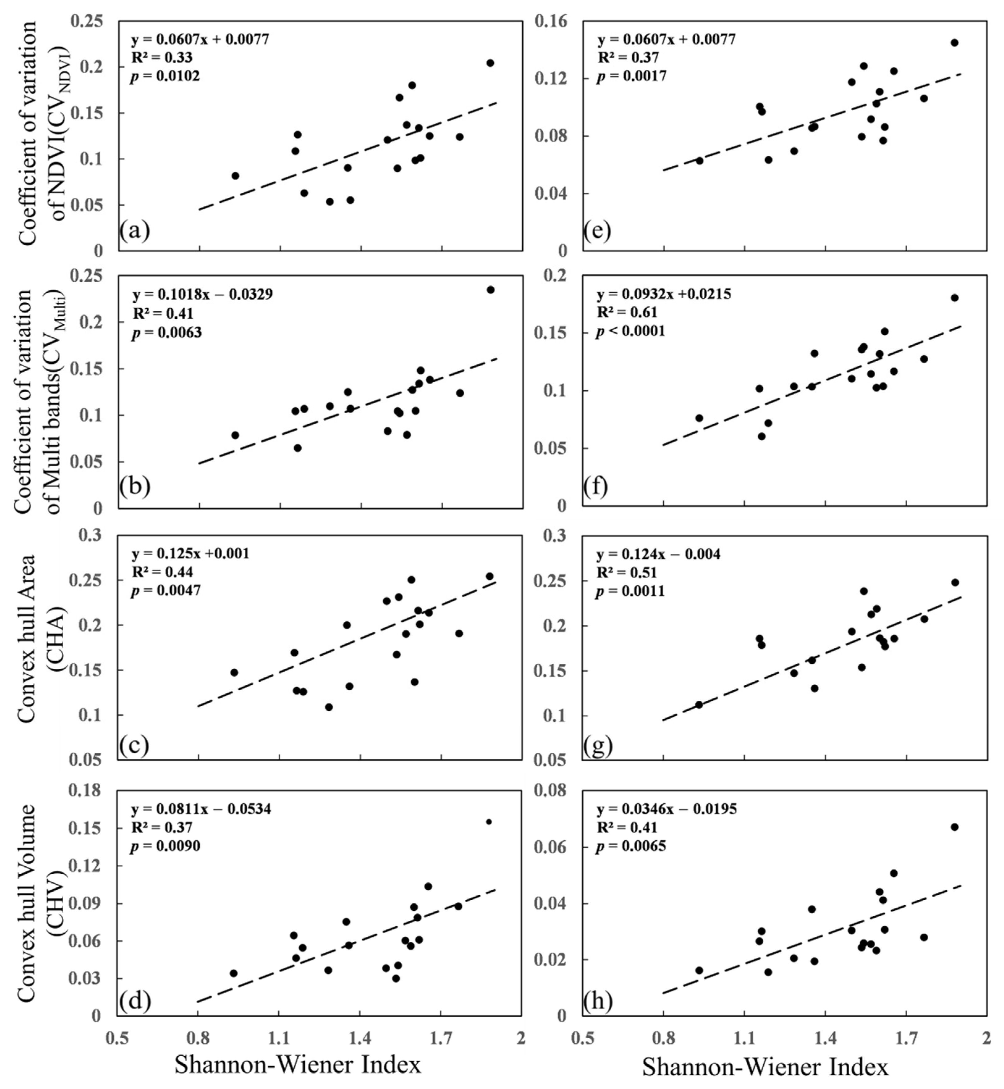
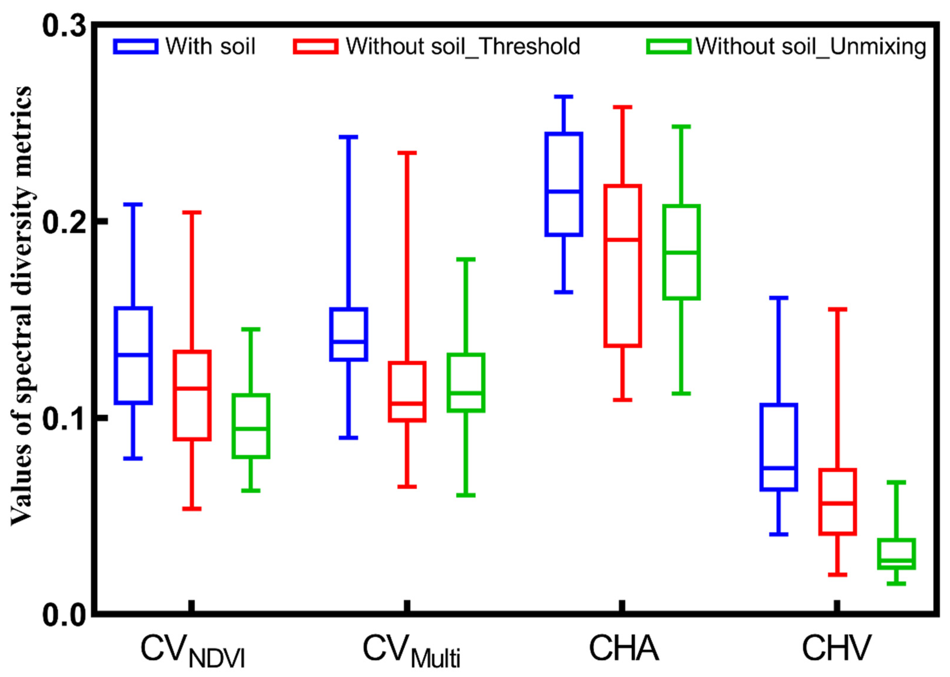
3.2. Impact of Soil on Spectral Diversity Metrics

We compared the relationships between the Shannon–Wiener index and spectral diversity calculated after soil removal using two methods. For the NDVI thresholds of soil removal, we finally used 0.4 for the following analysis due to its rigorousness for removing soil information after comparing the results of those three thresholds (Table 2). Obviously, the relationships between the Shannon–Wiener index and the four spectral diversity metrics were all improved after removing soil information (Figure 3). However, by filtering soil pixels based on NDVI threshold, the correlations between the Shannon–Wiener index and the four spectral diversity metrics had R2 from 0.33 to 0.44. In contrast, by extracting the vegetation information based on the inverted linear spectral unmixing model, the relationships between the Shannon–Wiener index and the four spectral diversity metrics had an R2 from 0.37 to 0.61, and CVMulti had the best performance (R2 = 0.61, Figure 3f).
Figure 4 shows that the median values of the 18 sample plots for the four spectral diversity metrics generally decreased after removing the soil. It demonstrates that the soil information might increase spectral heterogeneity to a certain extent, which leads to weaker relationships between spectral diversity metrics and species diversity. However, the maximum values of all spectral diversity metrics based on NDVI threshold had a slight change as the 0.4 threshold might not be suitable for soil removing of all sample plots. By contrast, the maximum values of spectral diversity metrics based on the linear spectral unmixing model showed an apparent reduction. Since the vegetation information of each pixel was extracted based on its various fractionals of vegetation coverage, rather than by a uniform threshold for all pixels, the linear spectral unmixing model could be more suitable for different grassland conditions. It demonstrated that the spectral diversity based on the linear spectral unmixing model had better performance at measuring the Shannon–Wiener index than when based on setting an NDVI threshold.
Additionally, the relationships between species richness and spectral diversity changed from nonsignificant to significant after soil removal (Table l), although the correlation between them still did not perform as well as the Shannon–Wiener index. This result also suggested that the soil information had a great effect on the response of spectral diversity to species diversity.
Based on the above results and analysis, after removing soil information by the linear spectral unmixing model, CVMulti was selected as the optimal spectral diversity metric to map the Shannon–Wiener index in this study area. We set a moving window with 5 × 5 pixels in order to match the sample plot of ground (1 m × 1 m) and calculate the regional CVMulti. Finally, the spatial distribution of the Shannon–Wiener index covering two UAV flight regions with 1 m spatial resolution was mapped and is shown in Figure 5.

4. Discussion

4.1. Methods for Grassland Species Diversity Estimation

Our findings demonstrated that the spectral variation hypothesis could be applied in the natural alpine steppe, and there was a significant positive correlation between spectral diversity and species diversity. We also highlighted that removing soil information in high-resolution UAV imaging spectroscopy data could improve the performance of spectral diversity metrics significantly, which was also observed in previous simulated and real-world grassland diversity studies [37,52]. Mixed pixels of soil and grass are ubiquitous in imaging spectroscopy data and soil information removal is a challenge. Compared with filtering soil or soil-dominant pixels by setting a fixed NDVI threshold, it is more suitable to remove soil information by the inverted linear spectral unmixing model (Figure 3). However, the spectral determination of pure soil is difficult since it is not easy to find the bare soil pixels in the natural alpine steppe, and the soil also has a variety of types over a large region. Therefore, multitemporal and hyperspectral remote sensing data could be considered in the future to extract each pixel with bare soil in the nongrowing season and accurately distinguish soil types with more spectral detail [74].
We used all bands from 390 nm to 1020 nm to calculate the spectral diversity metrics of CVMulti (R2 = 0.61), which performed much better than the CV of single band (R2 = 0.02~0.45) and CVNDVI (R2 = 0.37) to estimate the Shannon–Wiener index after soil removal based on the linear spectral unmixing model (Figure 6). It indicated that the multiple spectral bands could better explain the species heterogeneity than by a single band or certain VIs. However, the redundant and highly correlated bands still need deep analysis. For example, correlations and simple linear or random forest regression can be used for selecting the most important and nonredundant bands and PCA may be applied for extracting major axes to represent spectral heterogeneity. Additionally, the full spectral range from visible light (380–780 nm) to near infrared (780–2500 nm) could be further attempted to explore the effective band combinations.
The spectral heterogeneity essentially reflects the differences of grassland species in physiological and biochemical characteristics. Previous studies demonstrated that the many biochemical characteristics of grassland, usually considered as functional diversity, could be accurately estimated using remote sensing, such as chlorophyll a, b, β -carotene and lutein by visible bands, leaf nitrogen content and carbon content by near infrared bands and cellulose by shortwave infrared bands [75,76,77,78]. The ability of spectral diversity calculated based on the bands which might be sensitive to specific biochemical characteristics even exceeds that of NDVI for grassland diversity monitoring (Figure 6). With the relationships among spectral diversity, functional diversity and species diversity of grassland being further explored [35], the optimal functional components could also be used for indicating the species diversity.
Besides the biochemical characteristics, the functional diversity of grassland also includes the structural characteristics [45,79]. The vertical canopy structure even would mediate the link between spectral diversity and species diversity [80]. Although there are still uncertainties for obtaining grassland canopy structures, several structural characteristics of grassland have been estimated by terrestrial laser scanning. For instance, Guimarães-Steinicke et al. [81] regarded mean height and LAI as metrics of vertical structure, community stand gaps, canopy surface variation and emergent flowers as metrics of horizontal structure. Airborne or UAV-based LiDAR data could also be attempted to estimate the canopy structure characteristics of grassland over large areas [82]. However, the detection of grassland structure remains a challenge compared with forests, due to the more complex canopy structure and the smaller size of individual plants.
In addition, for the methods of mapping the species diversity of grassland, we usually consider the simple linear relationship between spectral diversity metrics and species diversity. Nevertheless, when the fundamental biochemical, structural and spectral characteristics related to the species diversity of grassland can be retrieved, a method of clustering by machine learning would be an alternative approach to monitor grassland diversity by remote sensing. For example, Zhao et al. [35] proposed a grassland species diversity estimation model that integrated the optimal biochemical components as functional diversity and spectral diversity based on the self-adaptive fuzzy c-means clustering algorithm.

4.2. Scales for Grassland Diversity Mapping

At the individual scale or leaf scale, spectral differences between species are enough to distinguish one species from another. However, it is difficult, in natural grassland, to separate individual tufts of different grassland species by some approaches applied in forests, such as the improved watershed algorithm [83,84]. Currently, most studies on grassland diversity mapping over a larger region were performed at pixel scale, just a few studies used proximal imaging spectrometry with millimeter resolution to estimate the species diversity of grassland, which was close to the individual scale [52,69]. Therefore, the spatial resolution of the acquired image and the scale of window used for estimation determine the accuracy of grassland species diversity mapping.
The commonly used Sentinel-2, Landsat TM and MODIS satellite data are mostly applied to retrieve different grassland biophysical parameters and estimate grassland types, communities or habitats by regression or classification model [85,86]. However, using these satellite data to monitor grassland species diversity based on spectral variation hypothesis is difficult, since the spectral variations are not just caused by species at such coarse spatial resolution [40]. The UAV or airborne data with spatial resolution in sub-meters provide the feasibility for estimating the α-diversity of the dominant species of grassland, which could also bridge the gaps between ground and satellite observations [36]. However, the mixture of several species within a pixel is the most common problem, even in this study by 0.2 m UAV data. Additionally, the individual size and structure of grassland plants also obviously varies between different grassland types, which exacerbates the problem of species mixing. Therefore, the optimal spatial resolution for monitoring grassland diversity at regional scale based on UAV or airborne still needs to be considered.
For the window scale of grassland diversity mapping, we used 5 × 5 pixels in this study due to the 1 m × 1 m size of thefield sample plots. Then, the simple linear relationships between spectral diversity and species diversity were demonstrated for species richness less than 10 and a Shannon–Wiener index less than 2 in each window. However, the spectral diversity could tend to reach saturation, due to the increasing species richness with upscaling the window size, which might be similar to the empirical power-law relationship between the species richness and area [87]. For example, Zhao et al. [35] found a tendency of gradual saturation based on the spectral characteristics when the species richness of grassland was above 17 within the estimation scale of 1.2 m × 1.2 m. Another study showed a contrary result that there was no saturated trend even when the species richness reached 50 within the windows of 60 m × 60 m, based on airborne data [32]. In addition, the window scale of diversity mapping is not only caused by the number of species, but also related to the environmental heterogeneity. Therefore, the optimal window scale for species diversity estimation in different study areas with different types of grassland and local environmental factors needs further study in the future by setting a gradient of window scale, especially for grassland with very high species richness.

5. Conclusions

In this study, we compared the relationships between four spectral diversity metrics and two species diversity indices, and further assessed the impact of soil on species diversity estimation based on UAV imaging spectroscopy in a natural alpine steppe in the Sanjiangyuan National Nature Reserve of China. We proved that spectral diversity metrics could be used to map grassland species diversity and the accuracy of estimation was improved effectively after removing soil information by the linear spectral unmixing model. Moreover, the Shannon–Wiener index and CVMulti were the better proxies of species diversity and spectral diversity, respectively. This result is conducive to bridging the scale gap for monitoring grassland species diversity from ground to near-ground by UAV data and provides a reference for assessing the impact of soil on species diversity estimation.
The UAV imaging spectroscopy and LiDAR technologies make it possible to monitor grassland species diversity at multiple perspectives and scales. These will also allow us to develop various methods and understand the scale differences caused by grassland itself and natural conditions. Further studies will explore the effectiveness of monitoring grassland species diversity based on more vegetation characteristics, which could be retrieved by remote sensing, such as biochemical and structural characteristics. Additionally, considering the variety of grassland types and their species, we suggest more attention should be paid to the applicability of the window scale and spatial resolution for grassland species diversity estimation, which would be a meaningful task for the accurate monitoring of grassland species diversity at a national or even global scale.

Author Contributions

Conceptualization, C.X. and Y.Z.; data curation, C.X.; formal analysis, C.X.; funding acquisition, Y.Z. and B.W.; investigation, C.X., D.Z. and W.L.; methodology, C.X. and Y.Z.; project administration, Y.Z.; resources, Y.Z.; software, C.X. and Z.M.; supervision, Y.Z.; validation, C.X., D.Z. and W.L.; visualization, C.X.; writing—original draft, C.X.; writing—review and editing, C.X., Y.Z., Z.Z. and D.Z. All authors have read and agreed to the published version of the manuscript.

Funding

This research was funded by the National Natural Science Foundation of China (No. 42071344).

Informed Consent Statement

Not applicable.

Data Availability Statement

Not applicable.

Conflicts of Interest

The authors declare no conflict of interest.

References

  1. Oliver, T.H.; Heard, M.S.; Isaac, N.J.B.; Roy, D.B.; Procter, D.; Eigenbrod, F.; Freckleton, R.; Hector, A.; Orme, C.D.L.; Petchey, O.L.; et al. Biodiversity and resilience of ecosystem functions. Trends Ecol. Evol. 2015, 30, 673–684. [Google Scholar] [CrossRef] [PubMed] [Green Version]
  2. Pan, Q.; Symstad, A.J.; Bai, Y.; Huang, J.; Wu, J.; Naeem, S.; Chen, D.; Tian, D.; Wang, Q.; Han, X. Biodiversity–productivity relationships in a natural grassland community vary under diversity loss scenarios. J. Ecol. 2021, 110, 210–220. [Google Scholar] [CrossRef]
  3. van Oijen, M.; Bellocchi, G.; Höglind, M. Effects of climate change on grassland biodiversity and productivity: The need for a diversity of models. Agronomy 2018, 8, 14. [Google Scholar] [CrossRef] [Green Version]
  4. Dirzo, R.; Raven, P.H. Global state of biodiversity and loss. Annu. Rev. Environ. Resour. 2003, 28, 137–167. [Google Scholar] [CrossRef] [Green Version]
  5. Linquist, S.; Varner, G.; Newman, J.E. Precis of defending biodiversity. Biol. Philos. 2020, 35, 14. [Google Scholar] [CrossRef]
  6. Cardinale, B.J.; Duffy, J.E.; Gonzalez, A.; Hooper, D.U.; Perrings, C.; Venail, P.; Narwani, A.; Mace, G.M.; Tilman, D.; Wardle, D.A.; et al. Biodiversity loss and its impact on humanity. Nature 2012, 486, 59–67. [Google Scholar] [CrossRef] [PubMed]
  7. Lu Yonglong, Y.Y.; Sun, B.; Yuan, J.; Yu, M.; Stenseth, N.C.; James, M.; Bullock, M.O. Spatial variation in biodiversity loss across china under multiple environmental stressors. Sci. Adv. 2020, 6, 11. [Google Scholar] [CrossRef]
  8. Harpole, W.S.; Sullivan, L.L.; Lind, E.M.; Firn, J.; Adler, P.B.; Borer, E.T.; Chase, J.; Fay, P.A.; Hautier, Y.; Hillebrand, H.; et al. Addition of multiple limiting resources reduces grassland diversity. Nature 2016, 537, 93–96. [Google Scholar] [CrossRef]
  9. Harrison, S.P.; Gornish, E.S.; Copeland, S. Climate-driven diversity loss in a grassland community. Proc. Natl. Acad. Sci. USA 2015, 112, 8672–8677. [Google Scholar] [CrossRef] [Green Version]
  10. Xu, H.; Cao, Y.; Yu, D.; Cao, M.; He, Y.; Gill, M.; Pereira, H.M. Ensuring effective implementation of the post-2020 global biodiversity targets. Nat. Ecol. Evol. 2021, 5, 411–418. [Google Scholar] [CrossRef]
  11. Hooper, D.U.; Chapin, F.S., III; Ewel, J.J.; Hector, A.; Inchausti, P.; Lavorel, S.; Lawton, J.H.; Lodge, D.M.; Loreau, M.; Naeem, S.; et al. Effects of biodiversity on ecosystem functioning: A consensus of current knowledge. Ecol. Monogr. 2005, 75, 3–35. [Google Scholar] [CrossRef]
  12. Isbell, F.; Gonzalez, A.; Loreau, M.; Cowles, J.; Diaz, S.; Hector, A.; Mace, G.M.; Wardle, D.A.; O’Connor, M.I.; Duffy, J.E.; et al. Linking the influence and dependence of people on biodiversity across scales. Nature 2017, 546, 65–72. [Google Scholar] [CrossRef] [PubMed] [Green Version]
  13. Lausch, A.; Bannehr, L.; Beckmann, M.; Boehm, C.; Feilhauer, H.; Hacker, J.M.; Heurich, M.; Jung, A.; Klenke, R.; Neumann, C.; et al. Linking earth observation and taxonomic, structural and functional biodiversity: Local to ecosystem perspectives. Ecol. Indic. 2016, 70, 317–339. [Google Scholar] [CrossRef]
  14. Lyashevska, O.; Farnsworth, K.D. How many dimensions of biodiversity do we need? Ecol. Indic. 2012, 18, 485–492. [Google Scholar] [CrossRef]
  15. Whittaker, R.H. Evolution and measurement of species diversity. Taxon 1972, 21, 213–251. [Google Scholar] [CrossRef] [Green Version]
  16. Harral, M.J.; Harral, J.E. Scale dependence in plant biodiversity. Science 2001, 291, 5. [Google Scholar] [CrossRef]
  17. Robert, J.; Whittaker, K.J.; Field, R. Scale and species richness: Towards a general, hierarchical theory of species diversity. J. Biogeogr. 2001, 18, 453–470. [Google Scholar] [CrossRef] [Green Version]
  18. Gaston, K.J. Global patterns in biodiversity. Nature 2000, 405, 8. [Google Scholar] [CrossRef]
  19. Shannon, C.E. A mathematical theory of communication. Bell Syst. Tech. J. 1948, 27, 379–423. [Google Scholar] [CrossRef] [Green Version]
  20. Magurran, A.E. Ecological Diversity and Its Measurement; Princeton University Press: Princeton, NJ, USA, 1988. [Google Scholar]
  21. Simpson, E.H. Measurement of diversity. Nature 1949, 163, 688. [Google Scholar] [CrossRef]
  22. Peet, R.K. The measurement of species diversity. Annu. Rev. Ecol. Syst. 1974, 5, 285–307. [Google Scholar] [CrossRef]
  23. Pielou, E.C. The measurement of diversity in diflerent types of biological collections. J. Theor. Biol. 1966, 13, 131–144. [Google Scholar] [CrossRef]
  24. Tilman, D.; Reich, P.B.; Knops, J.M. Biodiversity and ecosystem stability in a decade-long grassland experiment. Nature 2006, 441, 629–632. [Google Scholar] [CrossRef] [PubMed]
  25. Jochum, M.; Fischer, M.; Isbell, F.; Roscher, C.; van der Plas, F.; Boch, S.; Boenisch, G.; Buchmann, N.; Catford, J.A.; Cavender-Bares, J.; et al. The results of biodiversity-ecosystem functioning experiments are realistic. Nat. Ecol. Evol. 2020, 4, 1485–1494. [Google Scholar] [CrossRef] [PubMed]
  26. Mi, X.; Feng, G.; Hu, Y.; Zhang, J.; Chen, L.; Corlett, R.T.; Hughes, A.C.; Pimm, S.; Schmid, B.; Shi, S.; et al. The global significance of biodiversity science in china: An overview. Natl. Sci. Rev. 2021, 8, nwab032. [Google Scholar] [CrossRef]
  27. Pereira, H.M.; Ferrier, S.; Walters, M.; Geller, G.N.; Jongman, R.H.; Scholes, R.J.; Bruford, M.W.; Brummitt, N.; Butchart, S.H.; Cardoso, A.C.; et al. Ecology. Essential biodiversity variables. Science 2013, 339, 277–278. [Google Scholar] [CrossRef] [Green Version]
  28. Pettorelli, N.; Laurance, W.F.; O’Brien, T.G.; Wegmann, M.; Nagendra, H.; Turner, W.; Milner-Gulland, E.J. Satellite remote sensing for applied ecologists: Opportunities and challenges. J. Appl. Ecol. 2014, 51, 839–848. [Google Scholar] [CrossRef]
  29. Turner, W. Sensing biodiversity. Science 2015, 346, 301–304. [Google Scholar] [CrossRef]
  30. Turner, W.; Rondinini, C.; Pettorelli, N.; Mora, B.; Leidner, A.K.; Szantoi, Z.; Buchanan, G.; Dech, S.; Dwyer, J.; Herold, M.; et al. Free and open-access satellite data are key to biodiversity conservation. Biol. Conserv. 2015, 182, 173–176. [Google Scholar] [CrossRef] [Green Version]
  31. Buchanan, G.M.; Nelson, A.; Mayaux, P.; Hartley, A.; Donald, P.F. Delivering a global, terrestrial, biodiversity observation system through remote sensing. Conserv. Biol. 2009, 23, 499–502. [Google Scholar] [CrossRef]
  32. Gholizadeh, H.; Gamon, J.A.; Townsend, P.A.; Zygielbaum, A.I.; Helzer, C.J.; Hmimina, G.Y.; Yu, R.; Moore, R.M.; Schweiger, A.K.; Cavender-Bares, J. Detecting prairie biodiversity with airborne remote sensing. Remote Sens. Environ. 2019, 221, 38–49. [Google Scholar] [CrossRef]
  33. Gillespie, T.W.; Foody, G.M.; Rocchini, D.; Giorgi, A.P.; Saatchi, S. Measuring and modelling biodiversity from space. Prog. Phys. Geogr. Earth Environ. 2008, 32, 203–221. [Google Scholar] [CrossRef]
  34. Pettorelli, N.; Owen, H.J.F.; Duncan, C.; Freckleton, R. How do we want satellite remote sensing to support biodiversity conservation globally? Methods Ecol. Evol. 2016, 7, 656–665. [Google Scholar] [CrossRef]
  35. Zhao, Y.; Sun, Y.; Chen, W.; Zhao, Y.; Liu, X.; Bai, Y. The potential of mapping grassland plant diversity with the links among spectral diversity, functional trait diversity, and species diversity. Remote Sens. 2021, 13, 3034. [Google Scholar] [CrossRef]
  36. Rossi, C.; Kneubühler, M.; Schütz, M.; Schaepman, M.E.; Haller, R.M.; Risch, A.C.; Disney, M.; He, K. Spatial resolution, spectral metrics and biomass are key aspects in estimating plant species richness from spectral diversity in species-rich grasslands. Remote Sens. Ecol. Conserv. 2021, 1–18. [Google Scholar] [CrossRef]
  37. Wang, R.; Gamon, J.A.; Schweiger, A.K.; Cavender-Bares, J.; Townsend, P.A.; Zygielbaum, A.I.; Kothari, S. Influence of species richness, evenness, and composition on optical diversity: A simulation study. Remote Sens. Environ. 2018, 211, 218–228. [Google Scholar] [CrossRef]
  38. Palmer, M.W.; Earls, P.G.; Hoagland, B.W.; White, P.S.; Wohlgemuth, T. Quantitative tools for perfecting species lists. Environmetrics 2002, 13, 121–137. [Google Scholar] [CrossRef]
  39. Rocchini, D.; Bacaro, G.; Chirici, G.; Da Re, D.; Feilhauer, H.; Foody, G.M.; Galluzzi, M.; Garzon-Lopez, C.X.; Gillespie, T.W.; He, K.S.; et al. Remotely sensed spatial heterogeneity as an exploratory tool for taxonomic and functional diversity study. Ecol. Indic. 2018, 85, 983–990. [Google Scholar] [CrossRef] [Green Version]
  40. Schmidtlein, S.; Fassnacht, F.E. The spectral variability hypothesis does not hold across landscapes. Remote Sens. Environ. 2017, 192, 114–125. [Google Scholar] [CrossRef] [Green Version]
  41. Ustin, S.L.; Gamon, J.A. Remote sensing of plant functional types. New Phytol. 2010, 186, 795–816. [Google Scholar] [CrossRef]
  42. Cho, M.A.; Mathieu, R.; Asner, G.P.; Naidoo, L.; van Aardt, J.; Ramoelo, A.; Debba, P.; Wessels, K.; Main, R.; Smit, I.P.J.; et al. Mapping tree species composition in south african savannas using an integrated airborne spectral and lidar system. Remote Sens. Environ. 2012, 125, 214–226. [Google Scholar] [CrossRef]
  43. Schneider, F.D.; Morsdorf, F.; Schmid, B.; Petchey, O.L.; Hueni, A.; Schimel, D.S.; Schaepman, M.E. Mapping functional diversity from remotely sensed morphological and physiological forest traits. Nat. Commun. 2017, 8, 1441–1452. [Google Scholar] [CrossRef] [PubMed] [Green Version]
  44. Zhao, Y.; Zeng, Y.; Zheng, Z.; Dong, W.; Zhao, D.; Wu, B.; Zhao, Q. Forest species diversity mapping using airborne lidar and hyperspectral data in a subtropical forest in china. Remote Sens. Environ. 2018, 213, 104–114. [Google Scholar] [CrossRef]
  45. Zheng, Z.; Zeng, Y.; Schneider, F.D.; Zhao, Y.; Zhao, D.; Schmid, B.; Schaepman, M.E.; Morsdorf, F. Mapping functional diversity using individual tree-based morphological and physiological traits in a subtropical forest. Remote Sens. Environ. 2021, 252, 1–16. [Google Scholar] [CrossRef]
  46. Klingler, A.; Schaumberger, A.; Vuolo, F.; Kalmár, L.B.; Pötsch, E.M. Comparison of direct and indirect determination of leaf area index in permanent grassland. PFG—J. Photogramm. Remote Sens. Geoinf. Sci. 2020, 88, 369–378. [Google Scholar] [CrossRef]
  47. Lu, B.; He, Y. Species classification using unmanned aerial vehicle (uav)-acquired high spatial resolution imagery in a heterogeneous grassland. ISPRS J. Photogramm. Remote Sens. 2017, 128, 73–85. [Google Scholar] [CrossRef]
  48. Wachendorf, M.; Fricke, T.; Möckel, T. Remote sensing as a tool to assess botanical composition, structure, quantity and quality of temperate grasslands. Grass Forage Sci. 2018, 73, 1–14. [Google Scholar] [CrossRef]
  49. Wang, R.; Gamon, J.A. Remote sensing of terrestrial plant biodiversity. Remote Sens. Environ. 2019, 231, 111218. [Google Scholar] [CrossRef]
  50. Surfus, J.A.; Serrano, L.; Surfus, J.S. The photochemical refectance index: An optical indicator of photosynthetic radiation use efficiency across species, functional types, and nutrient levels. Oecologia 1997, 112, 492–501. [Google Scholar] [CrossRef]
  51. Dahlin, K.M. Spectral diversity area relationships for assessing biodiversity in a wildland–agriculture matrix. Ecol. Appl. 2016, 26, 11. [Google Scholar] [CrossRef]
  52. Gholizadeh, H.; Gamon, J.A.; Zygielbaum, A.I.; Wang, R.; Schweiger, A.K.; Cavender-Bares, J. Remote sensing of biodiversity: Soil correction and data dimension reduction methods improve assessment of α-diversity (species richness) in prairie ecosystems. Remote Sens. Environ. 2018, 206, 240–253. [Google Scholar] [CrossRef]
  53. Wang, R.; Gamon, J.; Emmerton, C.; Li, H.; Nestola, E.; Pastorello, G.; Menzer, O. Integrated analysis of productivity and biodiversity in a southern alberta prairie. Remote Sens. 2016, 8, 214. [Google Scholar] [CrossRef] [Green Version]
  54. Zhang, J.; Rivard, B.; Sánchez-Azofeifa, A.; Castro-Esau, K. Intra- and inter-class spectral variability of tropical tree species at la selva, costa rica: Implications for species identification using hydice imagery. Remote Sens. Environ. 2006, 105, 129–141. [Google Scholar] [CrossRef]
  55. Rocchini, D. Effects of spatial and spectral resolution in estimating ecosystem α-diversity by satellite imagery. Remote Sens. Environ. 2007, 111, 423–434. [Google Scholar] [CrossRef]
  56. Peng, Y.; Fan, M.; Bai, L.; Sang, W.; Feng, J.; Zhao, Z.; Tao, Z. Identification of the best hyperspectral indices in estimating plant species richness in sandy grasslands. Remote Sens. 2019, 11, 588. [Google Scholar] [CrossRef] [Green Version]
  57. Imran, H.A.; Gianelle, D.; Rocchini, D.; Dalponte, M.; Martín, M.P.; Sakowska, K.; Wohlfahrt, G.; Vescovo, L. Vis-nir, red-edge and nir-shoulder based normalized vegetation indices response to co-varying leaf and canopy structural traits in heterogeneous grasslands. Remote Sens. 2020, 12, 2254. [Google Scholar] [CrossRef]
  58. Gould, W. Remote sensing of vegetation, plant species richness, and regional biodiversity hotspots. Ecol. Appl. 2000, 10, 10. [Google Scholar] [CrossRef]
  59. Fauvel, M.; Lopes, M.; Dubo, T.; Rivers-Moore, J.; Frison, P.-L.; Gross, N.; Ouin, A. Prediction of plant diversity in grasslands using sentinel-1 and -2 satellite image time series. Remote Sens. Environ. 2020, 237, 111536. [Google Scholar] [CrossRef]
  60. Schweiger, A.K.; Cavender-Bares, J.; Townsend, P.A.; Hobbie, S.E.; Madritch, M.D.; Wang, R.; Tilman, D.; Gamon, J.A. Plant spectral diversity integrates functional and phylogenetic components of biodiversity and predicts ecosystem function. Nat. Ecol. Evol. 2018, 2, 976–982. [Google Scholar] [CrossRef]
  61. Lucas, K.; Carter, G. The use of hyperspectral remote sensing to assess vascular plant species richness on horn island, mississippi. Remote Sens. Environ. 2008, 112, 3908–3915. [Google Scholar] [CrossRef]
  62. Zhao, Y.; Sun, Y.; Lu, X.; Zhao, X.; Yang, L.; Sun, Z.; Bai, Y. Hyperspectral retrieval of leaf physiological traits and their links to ecosystem productivity in grassland monocultures. Ecol. Indic. 2021, 122, 107267. [Google Scholar] [CrossRef]
  63. Yu, X.; Guo, Q.; Chen, Q.; Guo, X. Discrimination of senescent vegetation cover from landsat-8 oli imagery by spectral unmixing in the northern mixed grasslands. Can. J. Remote Sens. 2019, 45, 192–208. [Google Scholar] [CrossRef]
  64. Zhou, X. Diversity of vascular plants in qinghai. J. Qinghai Environ. 2011, 4, 165–169. [Google Scholar] [CrossRef]
  65. Feng, M.; Che, X. Monthly surface water extent dataset for tibetan plateau and central asia (2000–2015). Natl. Tibet. Plateau Data Cent. 2019. [Google Scholar] [CrossRef]
  66. Li, C.; Peng, F.; Xue, X.; Lai, C.; Zhang, W.; You, Q.; Chen, X.; Zhang, X.; Wang, T. Degradation stage effects on vegetation and soil properties interactions in alpine steppe. J. Mt. Sci. 2021, 18, 646–657. [Google Scholar] [CrossRef]
  67. Wu, B.; Qian, J.; Zeng, Y. Land Cover Atlas of the People’s Re-Public of China (1:1,000,000); Sinomaps Press: Beijing, China, 2017. [Google Scholar]
  68. Yi, L.; Chen, J.M.; Zhang, G.; Xu, X.; Ming, X.; Guo, W. Seamless mosaicking of uav-based push-broom hyperspectral images for environment monitoring. Remote Sens. 2021, 13, 4720. [Google Scholar] [CrossRef]
  69. Lopatin, J.; Fassnacht, F.E.; Kattenborn, T.; Schmidtlein, S. Mapping plant species in mixed grassland communities using close range imaging spectroscopy. Remote Sens. Environ. 2017, 201, 12–23. [Google Scholar] [CrossRef]
  70. Oldeland, J.; Wesuls, D.; Rocchini, D.; Schmidt, M.; Jürgens, N. Does using species abundance data improve estimates of species diversity from remotely sensed spectral heterogeneity? Ecol. Indic. 2010, 10, 390–396. [Google Scholar] [CrossRef]
  71. Adams, J.B.; Smith, M.O.; Johnson, P.E. Spectral mixture modeling: A new analysis of rock and soil types at the viking lander 1 site. J. Geophys. Res. 1986, 91, 8098–8112. [Google Scholar] [CrossRef]
  72. Ding, Y.; Zheng, X.; Zhao, K.; Xin, X.; Liu, H. Quantifying the impact of ndvisoil determination methods and ndvisoil variability on the estimation of fractional vegetation cover in northeast china. Remote Sens. 2016, 8, 29. [Google Scholar] [CrossRef] [Green Version]
  73. Zeng, Y.; Schaepman, M.E.; Wu, B.; Clevers, J.G.P.W.; Bregt, A.K. Forest structural variables retrieval using eo-1 hyperion data in combination with linear spectral unmixing and an inverted geometric-optical model. J. Remote Sens. 2007, 11, 648–658. [Google Scholar]
  74. Li, F.; Zeng, Y.; Luo, J.; Ma, R.; Wu, B. Modeling grassland aboveground biomass using a pure vegetation index. Ecol. Indic. 2016, 62, 279–288. [Google Scholar] [CrossRef]
  75. Boegh, E.; Houborg, R.; Bienkowski, J.; Braban, C.F.; Dalgaard, T.; van Dijk, N.; Dragosits, U.; Holmes, E.; Magliulo, V.; Schelde, K.; et al. Remote sensing of lai, chlorophyll and leaf nitrogen pools of crop- and grasslands in five european landscapes. Biogeosciences 2013, 10, 6279–6307. [Google Scholar] [CrossRef] [Green Version]
  76. Kong, B.; Yu, H.; Du, R.; Wang, Q. Quantitative estimation of biomass of alpine grasslands using hyperspectral remote sensing. Rangel. Ecol. Manag. 2019, 72, 336–346. [Google Scholar] [CrossRef]
  77. Schiefer, F.; Schmidtlein, S.; Kattenborn, T. The retrieval of plant functional traits from canopy spectra through rtm-inversions and statistical models are both critically affected by plant phenology. Ecol. Indic. 2021, 121, 1–13. [Google Scholar] [CrossRef]
  78. Van Cleemput, E.; Vanierschot, L.; Fernández-Castilla, B.; Honnay, O.; Somers, B. The functional characterization of grass- and shrubland ecosystems using hyperspectral remote sensing: Trends, accuracy and moderating variables. Remote Sens. Environ. 2018, 209, 747–763. [Google Scholar] [CrossRef]
  79. Rossi, C.; Kneubühler, M.; Schütz, M.; Schaepman, M.E.; Haller, R.M.; Risch, A.C. From local to regional: Functional diversity in differently managed alpine grasslands. Remote Sens. Environ. 2020, 236, 111415. [Google Scholar] [CrossRef]
  80. Conti, L.; Malavasi, M.; Galland, T.; Komárek, J.; Lagner, O.; Carmona, C.P.; Bello, F.; Rocchini, D.; Šímová, P.; Feilhauer, H. The relationship between species and spectral diversity in grassland communities is mediated by their vertical complexity. Appl. Veg. Sci. 2021, 24. [Google Scholar] [CrossRef]
  81. Guimarães-Steinicke, C.; Weigelt, A.; Proulx, R.; Lanners, T.; Eisenhauer, N.; Duque-Lazo, J.; Reu, B.; Roscher, C.; Wagg, C.; Buchmann, N.; et al. Biodiversity facets affect community surface temperature via 3d canopy structure in grassland communities. J. Ecol. 2021, 109, 1969–1985. [Google Scholar] [CrossRef]
  82. Zhang, X.; Bao, Y.; Wang, D.; Xin, X.; Ding, L.; Xu, D.; Hou, L.; Shen, J. Using uav lidar to extract vegetation parameters of inner mongolian grassland. Remote Sens. 2021, 13, 656. [Google Scholar] [CrossRef]
  83. Zhao, D.; Pang, Y.; Li, Z.; Liu, L. Isolating individual trees in a closed coniferous forest using small footprint lidar data. Int. J. Remote Sens. 2014, 35, 7199–7218. [Google Scholar] [CrossRef]
  84. Zhao, D.; Pang, Y.; Li, Z.; Sun, G. Filling invalid values in a lidar-derived canopy height model with morphological crown control. Int. J. Remote Sens. 2013, 34, 4636–4654. [Google Scholar] [CrossRef]
  85. Ali, I.; Cawkwell, F.; Dwyer, E.; Barrett, B.; Green, S. Satellite remote sensing of grasslands: From observation to management. J. Plant Ecol. 2016, 9, 649–671. [Google Scholar] [CrossRef] [Green Version]
  86. Rapinel, S.; Mony, C.; Lecoq, L.; Clément, B.; Thomas, A.; Hubert-Moy, L. Evaluation of sentinel-2 time-series for mapping floodplain grassland plant communities. Remote Sens. Environ. 2019, 223, 115–129. [Google Scholar] [CrossRef]
  87. Dolnik, C.; Breuer, M. Scale dependency in the species-area relationship of plant communities. Folia Geobot. 2008, 43, 305–318. [Google Scholar] [CrossRef]
Figure 1. The location of Sanjiangyuan National Nature Reserve (left), Maduo county (middle) with land cover data with 10 m spatial resolution from ChinaCover2020 [67], and two UAV imaging spectroscopy images (NIR: 860 nm, red: 660 nm, green: 560 nm) with 18 field-measured sample plots and photographs (right).
Remotesensing 14 00671 g001
Figure 2. The relationships between species diversity and spectral diversity with soil information. The left column indicates the relationships between four spectral diversity metrics and species richness (ad) and the right column indicates the relationships between four spectral diversity metrics and Shannon–Wiener index (eh).
Remotesensing 14 00671 g002
Figure 3. The relationship between Shannon–Wiener index and spectral diversity without soil information. The left column indicates the relationship between Shannon–Wiener index and four spectral diversity metrics after removing the soil based on the NDVI threshold (NDVI threshold is 0.4. (ad); The right column represents the relationship between Shannon–Wiener index and four spectral diversity metrics after removing the soil based on the linear spectral unmixing model (eh).
Remotesensing 14 00671 g003
Figure 4. The variation of four spectral diversity metrics between 18 sample plots before and after soil information removal. Each box shows the maximum, the upper quartile, the mean, the lower quartile and the minimum. Each spectral diversity metric includes three conditions: with soil information (blue), without soil information, removed by setting NDVI threshold (red) and without soil information, removed by linear spectral unmixing model (green).
Remotesensing 14 00671 g004
Figure 5. Predicted Shannon–Wiener index with a spatial resolution of 1 m in the natural grassland of UAV flight region 1 (left) and UAV flight region 2 (right).
Remotesensing 14 00671 g005
Figure 6. The coefficient of determination (R2) of Shannon-Wiener index and CV calculated by each single band from 390 nm to 1020 nm, R2 = 0.61 (CVMulti) and 0.37 (CVNDVI) were tagged as blue and green horizontal lines.
Remotesensing 14 00671 g006
Table 1. The correlations between species diversity indices and spectral diversity metrics before and after removing soil information based on two methods in terms of R2, p-value, RMSE and bias.
Spectral DiversitySoil FilteringSpecies RichnessShannon–Wiener Index
R2p-ValueRMSEBiasR2p-ValueRMSEBias
CVNDVIWith soil0.130.123.400.240.240.03 *0.390.08
NDVI threshold0.290.02 *2.270.110.330.01 **0.170.07
Unmixing0.280.007 **2.250.090.370.002 **0.080.04
CVMultiWith soil0.100.173.760.310.260.03 *0.150.07
NDVI threshold0.340.02 *1.890.080.410.006 **0.070.04
Unmixing0.400.002 **1.740.070.61<0.001 **0.040.02
CHAWith soil0.190.072.940.170.280.003 **0.140.06
NDVI threshold0.360.01 *1.880.080.440.005 **0.070.03
Unmixing0.400.005 **1.770.070.510.001 **0.060.03
CHVWith soil0.160.083.240.200.240.04 *0.170.07
NDVI threshold0.240.04 *2.400.120.370.009 **0.090.04
Unmixing0.290.03 *2.180.100.410.007 **0.080.03
Notes: *, 0.01 < p-value < 0.05, significant; **, p-value < 0.01, extremely significant. With soil represents spectral diversity metrics before soil removal; NDVI threshold represents spectral diversity metrics after soil removal based on NDVI threshold; unmixing represents spectral diversity metrics after soil removal based on linear spectral unmixing model.
Table 2. The correlations between species diversity indices and spectral diversity metrics after removing soil information based on three NDVI thresholds in terms of R2, p-value, RMSE and bias.
Spectral DiversityNDVI ThresholdSpecies RichnessShannon–Wiener Index
R2p-ValueRMSEBiasR2p-ValueRMSEBias
CVNDVI0.20.27 *0.03 *5.160.110.33 *0.01 *0.170.08
0.30.27 *0.03 *5.150.110.33 **0.009 **0.180.08
0.40.29 *0.02 *5.150.110.33 **0.01 **0.170.07
CVMulti0.20.27 *0.03 *3.980.100.41 **0.006 **0.080.04
0.30.28 *0.03 *3.900.100.41 **0.006 **0.080.04
0.40.34 *0.02 *3.570.080.41 **0.006 **0.070.04
CHA0.20.28 *0.03 *4.130.100.42 **0.004 **0.080.03
0.30.33 *0.02 *3.860.090.40 **0.005 **0.090.04
0.40.36 *0.01 *3.530.080.44 **0.005 **0.070.03
CHV0.20.22 *0.03 *6.040.130.35 **0.008 **0.080.04
0.30.24 *0.02 *5.740.110.35 **0.009 **0.080.04
0.40.24 *0.04 *5.760.120.37 **0.009 **0.090.04
Notes: *, 0.01 < p-value < 0.05, significant; **, p-value < 0.01, extremely significant.
Publisher’s Note: MDPI stays neutral with regard to jurisdictional claims in published maps and institutional affiliations.

