Article

Classifying Individual Shrub Species in UAV Images—A Case Study of the Gobi Region of Northwest China

Institute of Desertification Study, Chinese Academy of Forestry, Beijing 100091, China
*
Author to whom correspondence should be addressed.
Remote Sens. 2021, 13(24), 4995; https://doi.org/10.3390/rs13244995
Submission received: 27 October 2021 / Revised: 1 December 2021 / Accepted: 6 December 2021 / Published: 8 December 2021
(This article belongs to the Special Issue Remote Sensing of Ecosystems)

Abstract

:
Shrublands are the main vegetation component in the Gobi region and contribute considerably to its ecosystem. Accurately classifying individual shrub vegetation species to understand their spatial distributions and to effectively monitor species diversity in the Gobi ecosystem is essential. High-resolution remote sensing data create vegetation type inventories over large areas. However, high spectral similarity between shrublands and surrounding areas remains a challenge. In this study, we provide a case study that integrates object-based image analysis (OBIA) and the random forest (RF) model to classify shrubland species automatically. The Gobi region on the southern slope of the Tian Shan Mountains in Northwest China was analyzed using readily available unmanned aerial vehicle (UAV) RGB imagery (1.5 cm spatial resolution). Different spectral and texture index images were derived from UAV RGB images as variables for species classification. Principal component analysis (PCA) extracted features from different types of variable sets (original bands, original bands + spectral indices, and original bands + spectral indices + texture indices). We tested the ability of several non-parametric decision tree models and different types of variable sets to classify shrub species. Moreover, we analyzed three main shrubland areas comprising different shrub species and compared the prediction accuracies of the optimal model in combination with different types of variable sets. We found that the RF model could generate higher accuracy compared with the other two models. The best results were obtained using a combination of the optimal variable set and the RF model with an 88.63% overall accuracy and 0.82 kappa coefficient. Integrating OBIA and RF in the species classification process provides a promising method for automatic mapping of individual shrub species in the Gobi region and can reduce the workload of individual shrub species classification.

Graphical Abstract

1. Introduction

Shrubs are dominant plants in the extremely arid Gobi region of China [1]. Shrub vegetation patches are the main components of shrub communities [2]. The shrub species and their spatial distributions reflect the species composition of a shrub community and the spatial configurations of different species, both of which are fundamental indices in ecological research and key metrics in vegetation surveys of the Gobi region [3,4]. Although actual individual shrub species and spatial distribution data can be obtained using traditional field survey methods (i.e., line transects, quadrats, and belt transects) [5], it is difficult to accurately monitor shrub vegetation communities at a landscape scale because traditional field methods obtain data from plant communities at small scales. It is also more difficult and time-consuming to conduct field surveys at the scale of a single plant in areas with harsh natural conditions (e.g., the Gobi Desert) and data omissions may occur [6], which leads to uncertainties in the analytical results for species composition and the spatial distribution of shrub communities in such regions.
Over the past few decades, an increasing number of studies have been conducted on the identification and spatial distributions of vegetation species using remote sensing technology [7,8,9,10,11]. Most of these studies have focused on species classification at the landscape scale in forest, wetland, and tropical rainforest regions based on high, medium, and low spatial resolution satellite remote sensing data. Few studies have been conducted on species classification in the Gobi region. Most shrubs found in this region are sparse and less diverse than in forests, thereby increasing the difficulty of detecting them with satellite remote sensing technology and restricting its application. Fortunately, remote sensing technology is developing towards the generation and application of data with a high temporal and spatial resolution [12]. In recent years, the application of unmanned aerial vehicles (UAVs) for remote sensing in vegetation resource surveys and ecological research has improved significantly due to their high spatial resolution, speed, low cost, and reusability [13]. This has enabled the high-resolution classification of individual vegetation species in UAV images, as well as rapid mapping of spatial vegetation distributions in the Gobi region at a landscape scale.
Remotely sensed data obtained using UAVs have mainly included light detection and ranging (Lidar) point clouds, hyperspectral images, multispectral images, and RGB images [14,15,16]. In general, vegetation species classification based on Lidar point clouds is achieved using a range of features related to tree structures. For instance, the geometric part of Lidar data have been used to detect the architecture of tree crowns [17], while the intensity of the backscattered signal can be used to differentiate foliage type [18] and leaf size [19]. Classification of vegetation species based on aerial multispectral images and hyperspectral images is accomplished by combining spectral features with spatial features [16,20,21]. However, deriving the architecture of crowns from Lidar data requires extremely high-quality point cloud data when the local surface vegetation is less than 2 m tall, which makes data collection in the Gobi area difficult where sparse shrubs are only 15 cm high [5]. In addition, the high cost and complicated data processing related to hyperspectral images have seriously hindered their application and popularity [22]. In contrast, the common digital camera sensors carried by UAV have wider application prospects because they are inexpensive and can quickly acquire high spatial resolution RGB images [23]. Although they lack the three-dimensional information of a Lidar point cloud and the detailed spectral information contained in multispectral or hyperspectral images, their spatial structure feature is quite robust [24]. Recently, various non-parametric decision tree algorithms, including support vector machine (SVM), random forest (RF), and kernel nearest neighbor (k-NN), have been most used to classify vegetation species based on UAV RGB images [25,26,27,28]. The RF algorithm, also known as machine learning, is an integrated model that builds decision trees by randomly selecting variables and training sample data [29,30]. It is regarded as the optimal classification model for remote sensing data in areas with complex environments and noise because of its high predictive stability and classification accuracy compared to other traditional classification models [31,32].
Establishing feature sets is the basis for vegetation species classification [33,34]. The UAV RGB images are composed of three bands (red, green, and blue), each of which has a high resolution. Therefore, the effective utilization of the spectral data and the spatial structural features of UAV RGB images are critical for accurately classifying vegetation species. Spectral indices are often used to identify vegetation features. Currently, various spectral indices (i.e., excess blue index (ExB), visible atmospherically resistant index (VARI), and red blue ratio index (RBRI)) have been developed for UAV RGB images [35]. Some studies have successfully used different spectral indices to distinguish dominant species from non-dominant species in desert areas and extract their location information [5,36]. However, due to the spectral heterogeneity and spatial complexity of the target area, classifying vegetation species using one or more simple spectral indices is complex [37,38]. With the advance in machine vision and pattern recognition technology, crown texture features have become more meaningful for classifying vegetation species [39,40,41]. Crown texture features are helpful for distinguishing species with small spectral differences but different canopy surface structures [42]. Textural features of images are commonly quantified by Gray-level co-occurrence matrix (GLCM) indices, which are fundamental indices in image texture analysis because of their ability to capture changes in objects with different textures, including smooth, irregular, or bumpy tree crowns and grasses [43]. Each index can highlight specific texture properties, such as smoothness, convexity, and irregularity, which can improve the classification accuracy of different objects [44]. In previous studies, eight GLCM indices (mean, variance, correlation, contrast, dissimilarity, homogeneity, energy, and entropy) have been used to characterize the landscape patterns of urban canopies, results of which have shown that GLCM indices can effectively represent the textural and structural characteristics of different canopy types [45]. In addition to these derived spectral or textural indices, complementary variables such as digital elevation models, digital surface models, etc., have been used for complex classification tasks.
Ideally, the classification accuracy increases with more variables [46]. However, issues such as high variable correlation and increased computational complexity can undermine the classification accuracy and efficiency [47]. Therefore, it is necessary to find a feature subset that can balance the prediction accuracy and model efficiency. Principal component analysis (PCA) can be used for feature extraction and data dimensionality reduction. In remote sensing image classification tasks, PCA transforms input bands to generate a new set of uncorrelated variables, which have reduced dimensionality while retaining the essential information [48]. The resulting principal component (PC) band is a combination of input bands. PC bands containing the main information can be used directly for remote sensing image classification instead of the original bands [49].
Previous studies of vegetation species classification have mainly focused on stand scale classification, and the study objects have generally been pure or mixed forests of artificially planted trees that were aggregated and had high densities [11,50,51,52]. However, few studies have classified the species of individual plants growing in original shrub vegetation communities in the Gobi region. A few studies have focused on the canopy segmentation of a single plant, and the research targets have generally been tall tree species [53]. The surface of the Gobi region comprises sparse shrub vegetation patches, Gobi gravel, and heterogeneous soil patches. Due to the long-term impact of environmental factors, such as dust weather and water limitations, the vegetation community types in the Gobi region are quite different: the plants are short and sparse, and their growth varies significantly. In high spatial resolution UAV RGB images obtained from this area, the changes in noise, light, and spectral resolution in the image background and within the plant canopy increase the heterogeneity among the pixels, which has a large negative impact on the classification results and increases the difficulty of species classification based on the image pixels.
Object-based image analysis (OBIA) has great potential for addressing this issue [54,55]. OBIA uses homogeneous areas of the image, which replace individual pixels as the basic elements of image analysis. Simultaneously, the texture features of the region can be used for classification [56]. This method includes two parts: image segmentation and classification. More accurate classification of vegetation species can be achieved with an appropriate image segmentation algorithm. Multi-scale segmentation is a widely used bottom-up algorithm that combines adjacent pixels to form homogeneous and adjacent objects (blocks) by adjusting different parameters to minimize the average difference between the objects [57]. The multi-scale segmentation parameters include scale, shape, and tightness. Studies have shown that varying segmentation parameters greatly affects the quality of the image segmentation [58,59]. When processing high spatial resolution images of vegetation, OBIA directly classifies the segmented vegetation canopy to lower the negative effect of pixel spectral changes, thereby capturing multi-pixel vegetation targets more effectively than single pixel-based classification and obtaining more accurate classification results [54]. Previous research has shown that the OBIA method is superior to the pixel-based classification method for classifying vegetation species, particularly in high spatial resolution images [60].
Taking into account challenges of classifying individual shrub species at a fine scale and rapidly mapping their spatial distributions in the complex surface environment of the Gobi region, as well as the impacts of different classification methods and variable sets on species classification accuracy, this study aimed to: (1) test the shrub species classification capabilities of several non-parametric decision tree classifiers and different sets of variables with UAV RGB images of the Gobi area to determine the optimal classifier with the best set of variable; (2) integrate this optimal classifier with OBIA to develop a reliable strategy for shrub species classification based on UAV RGB images of the Gobi region; and (3) classify shrub species in the Gobi region using the optimal classifier and reveal spatial patterns of shrub species at different locations in the Gobi region.

2. Materials and Methods

2.1. Study Area

The study area (41.840518–42.061273° N, 83.84486–84.212092° E) is located in the Gobi region in northern Luntai County, Xinjiang, China (Figure 1). This region is composed of alluvial fans of different sizes that were formed by seasonal rivers, which is a typical landscape type in the Gobi region. The study area has a typical continental climate in the middle temperate zone that is characterized by arid conditions, little rain, and high evaporation. Precipitation mostly occurs from June to August, with average annual precipitation and evaporation of 47.4 and 2082 mm, respectively. The study area covers an area of ~374 km2, with an altitude range of 1050–1350 m and a slope range of 0–10°. The ground surface in the study region consists primarily of Gobi gravel and soil crusts, with hard soil surfaces. These topographic and climatic conditions have contributed to the formation of a unique Gobi shrub vegetation community.
The Gobi region is mainly covered by bare land with sparsely distributed vegetation composed of shrub species (e.g., Ephedra przewalskii, Salsola laricifolia, Sarcozygium xanthoxylon, Gymnocarpos przewalskii, and Reaumuria songarica). Four vegetation alliances (namely EPPR, EPPR–SAXA–GYPR, EPPR–SALA–GYPR, and EPPR–SALA) represent the dominant habitat types. These four alliances are the dominant habitats of Ephedra przewalskii and exhibit a repetitive pattern of shrubs throughout the landscape. The EPPR consists entirely of Ephedra przewalskii. EPPR–SAXA–GYPR is the main shrub species-dominant habitat that includes Ephedra przewalskii, Sarcozygium xanthoxylon, and Gymnocarpos przewalskii. The EPPR–SALA habitat consists of Ephedra przewalskii and Salsola laricifolia. The EPPR–SALA–GYPR habitat is composed of Ephedra przewalskii, Salsola laricifolia, and Gymnocarpos przewalskii.

2.2. Field Sampling Data

Field surveys were conducted from July to September in 2018, 2019, and 2020 (vegetation-growing season). We developed four survey transects within the study area by referring to a four-band (red, green, blue, and near-infrared; NIR) high-resolution satellite image obtained in 2018. Six representative 100 × 100 m plots were positioned along each transect, parallel to the elevation gradient. In addition, to maintain the uniformity of the vegetation survey, we randomly selected another 14 plots. In total, we analyzed 38 sample plots that covered all of the vegetation alliance types. The distribution of sampling locations is shown in Figure 2.
A Hemisphere S320 GPS (Hemisphere GNSS, Inc., Calgary, AB, Canada) device with ±10 mm horizontal precision was used to collect the location information at each plot. The GPS location, shrub species, shrub height, crown breadth, and survival status of each shrub within the plot areas were also recorded simultaneously. Based on the plot data collected in 2018, we delineated the vegetation alliances in the study area and designed a species classification scheme that included four different shrub species category. During the three years (2018 to 2020) of field investigations in the study area, we did not find any significant changes in the spatial distributions of the vegetation alliances and shrub species. Therefore, in this study, we assumed that vegetation alliances are unvarying.

2.3. Acquisition and Pre-Processing of UAV RGB Images

UAV images were acquired at 60 m ground height between time points 12:00 and 14:00 in July 2018 under fine weather conditions. The DJI Phantom 4pro UAV (DJI-Innovations, Shenzhen, China) was used for high quality RGB image collection, which uses a quadrotor flight system that integrates a waypoint navigation system and a digital camera. The camera was set to shoot the plots vertically, resulting in 194 raw images per plot at an average pixel size of 1.5 cm. The forward overlap was 70% and the side overlap was 80%. A total of 38 survey flights were conducted, covering all of the 100 × 100 m plots. We measured five ground control points (GCP) at each plot and used GPS to georeference the images.
UAV image pre-processing was performed using the Agisoft PhotoScan software (Agisoft LLC, Petersburg, Russia), which uses the structure from motion algorithm to extract features that appear in a series of overlapping images. Each feature point was georeferenced using the ground control points, after which high-resolution orthomosaics were exported for each of the RGB bands. A total of 38 plots were produced from the UAV RGB orthomosaics. Example results of pre-processing are shown for three plots in Figure 2, which clearly shows morphological characteristics and species information for shrubs. Figure 3 shows ground-based field survey photos of the different shrub species and their corresponding UAV images.

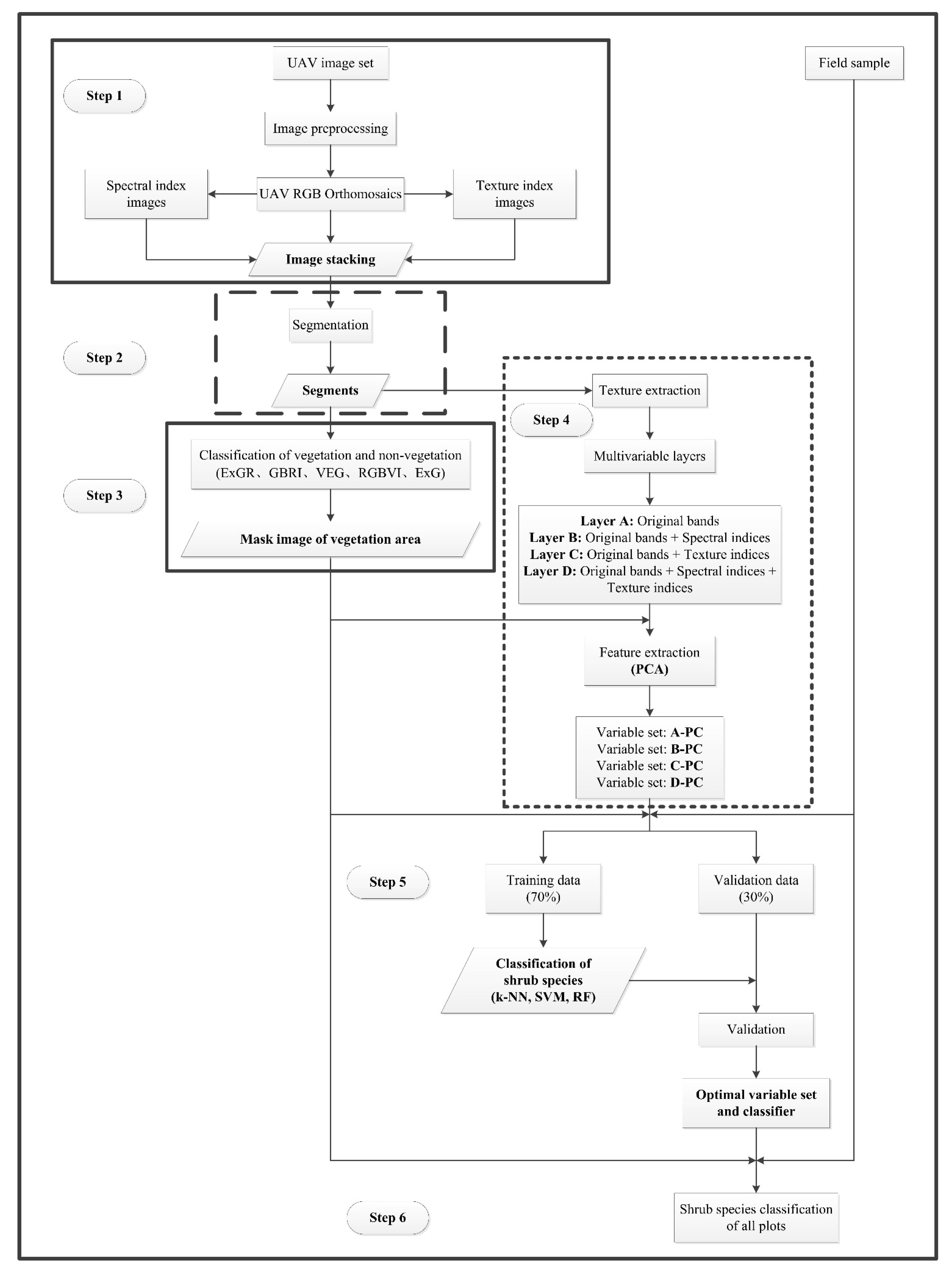
2.4. Fine Scale Classification of Individual Shrub Species

2.4.1. UAV RGB Image Segmentation

Figure 4 shows the workflow for classification of individual shrub species. When the input data pixel size (in this case, 1.5 cm) is smaller than the size of the vegetation patches, an OBIA approach is recommended [54,61,62,63]. This approach consists of two parts: image segmentation and classification. Multi-scale segmentation is a region-based segmentation method that merges a pixel with adjacent pixels to create homogeneous and contiguous segments [34]. This method includes three parameters (scale, shape, and tightness) that can each affect the results. We used the multi-scale segmentation method to implement image segmentation prior to shrub species classification in this study. Canopy crowns of the different shrub species in the study area differ; therefore, to avoid over or under-segmentation, we considered the canopy segmentation as the main principal and used the visual discriminant method to determine the optimal segmentation parameters. The multi-scale segmentation of all UAV images was conducted using the eCognition Developer 9 software (Trimble Inc., Munich, Germany).

2.4.2. Variable Derivation for Classification

Referring to previous studies of spectral and textural indices [24,33,45,64,65,66,67,68,69,70,71,72], we defined two categories of features that included both the original spectral bands (three bands) and spectral and textural indices derived from the UAV RGB images, and used them to characterize the spectral and textural features of the images. In addition, we carefully considered other features that are helpful for image classification based on a literature review (Appendix B, Table A3).
In this study, we obtained 23 derived indices based on three RGB bands (Appendix B, Table A3). Additionally, we calculated eight GLCM indices (mean, variance, homogeneity, contrast, dissimilarity, entropy, energy, and correlation) (Appendix A, Table A1) using the blue, green, and red bands. Next, 24 texture variables were generated. For all of the variables, we calculated the mean and standard deviation for all segments. All of the derived variables were stacked together with the original bands (RGB) to construct a new layer with 100 variable sets for classification. The variable sets used for shrub species classification were divided into four types, namely: (A) original bands (Red, Green, and Blue bands), (B) original bands + all derived spectral bands, (C) original bands + all derived texture bands, and (D) original bands + all derived spectral bands + all derived texture bands. Analyses were performed in R (R Core Team, R Foundation for Statistical Computing, Vienna, Austria), ENVI 5.3 (Exelis VIS, Boulder, CO, USA), and ArcGIS 10.7 (ESRI, Redlands, CA, USA).
PCA was used to decorrelate the data and reduce the dataset dimension of the four sets of variables. This method eliminates the duplication of information shared between different variables. The number of variables resulting from PCA is the same as the number of input variables. In addition, eigenvalues are used to identify useful components. In general, the first three components contain most of the information. The first PCA band includes the widest percentage of the data variance, while the later PCA bands contain more noise [48]. In this study, the A-PC, B-PC, C-PC, and D-PC represent the sets of variables used in the classification experiments of shrub species after principal component analysis (PCA) of variable sets A, B, C, and D, respectively. Since this research only focused on shrub vegetation, the non-vegetation pixels were masked out during PCA. The mask images were extracted based on the visible vegetation index. See Section 2.4.4 for specific implementation of this process.

2.4.3. Training and Testing Data Construction

The locations and species information of single shrubs within the plot areas collected in 2018 and 2019 were imported into the ArcGIS 10.7 software as ground reference sampling points to construct training and testing datasets for shrub species classification and accuracy verification. Based on the species classification scheme that included four shrub species, and the density of the species we investigated, samples with different sizes were selected for each shrub species. In total, 2991 random segments (which correspond to the ~4% of the total segments, Table 1) segmented from UAV images of three vegetation alliances were selected. These segments were then divided into two datasets (including the 70% (2094 segments) and 30% (897 segments) of segments) using a random stratified sampling approach for training and testing procedures (accuracy assessment). The class names and their descriptions are presented in Table 1.

2.4.4. Shrub Species Classification

In the classification step, segments generated from the UAV images of shrub vegetation alliances formed the basic units for classification. In order to exclude the influence of background information on shrub species classification, five commonly used visible vegetation indices (excess green red index (ExGR), green blue ratio index (GBRI), vegetative index (VEG), red green blue vegetation index (RGBVI), excess green index (ExG)) were combined with a fixed threshold classification method to extract vegetation and non-vegetation segments. We first determined classification thresholds of vegetation and non-vegetation feature types using the mean value of each index. Plant regions of interest were then binarized using a selected threshold value for all segments. Segments with a mean vegetation index greater than the optimal threshold values were classified as vegetation, and were otherwise classified as non-vegetation [73]. After comparing the vegetation and non-vegetation classification accuracy of five vegetation indices, we used the one with the highest classification accuracy to divide all images into vegetation and non-vegetation segments. Detailed vegetation classification was then conducted based on the confirmed class of vegetation. The vegetation and non-vegetation mask images were also applied to improve the classification efficiency.
Notably, different combinations of variables in the dataset will lead to deviations in the classification results, and could affect the computational efficiency and model accuracy. In this study, we conducted four classification experiments with different types (A-PC, B-PC, C-PC, and D-PC) of variable sets to analyze the influence of different types of derived variable sets (spectral indices and texture indices) on species classification. Moreover, we compared the classification accuracy for both RF, SVM, and k-NN classifiers to select the top model with optimal variable set and classifier. The classification was completed using 2094 training samples in the R package ‘caret’ [74].
Three classifiers were used to classify segments from four stacked variable sets into shrub species types. The k-NN classifier uses the observed Euclidean distance to classify it to the nearest training sample observation and assign it to the class. It is usually used for single tree detection in forests [28,75]. The SVM classifier has strong robustness to noise and high-dimensional data, requires relatively little training data, is widely used in tree species classification, and is suitable for complex canopy vegetation [25,75]. The default parameters of the caret package were used in SVM and k-NN classifiers. The RF classifier provides two decision tree models (classification regression tree (CART) and conditional inference tree) to perform the classification. CART is a binary tree for recursive partitioning, and the CART based random forest (CART-RF) model tends to generate higher classification accuracies [46]. CART-RF required two parameters: the number of features inside the set (mtry) and the overall number of trees (ntree). Both parameters for the CART-RF model were selected by testing them with 10-fold cross validation on the training data. To optimize the two parameters, we set the ntree value to 500, and tested it with the mtry values used in [3,9]. We then chose the combination of values that yielded the highest accuracy (ntree = 500 and mtry = 7).
After obtaining the optimal classification variable set and the top classification model, we classified shrub species from UAV images of 38 survey plots and counted the number and area of species in each plot.

2.4.5. Classification Model Validation

We first evaluated the vegetation and non-vegetation results extracted by five vegetation indices using the overall accuracy (OA) and Kappa coefficient and identified the vegetation index with the highest vegetation classification accuracy. Thereafter, we compared the accuracy of different types of variable sets in three classification models to assess the contributions of the derived indices (spectral indices and texture indices) and the shrub species classification capabilities of different models in the Gobi region. In this step, a confusion matrix was constructed using the 897 independent test segments (30% of the segments). The selected accuracy indicators included OA, user accuracy (UA), producer accuracy (PA), and the Kappa coefficient (Appendix A, Table A2). In addition, we also visually compared the shrub species classification maps of four types of variable sets generated by the optimal model.

3. Results

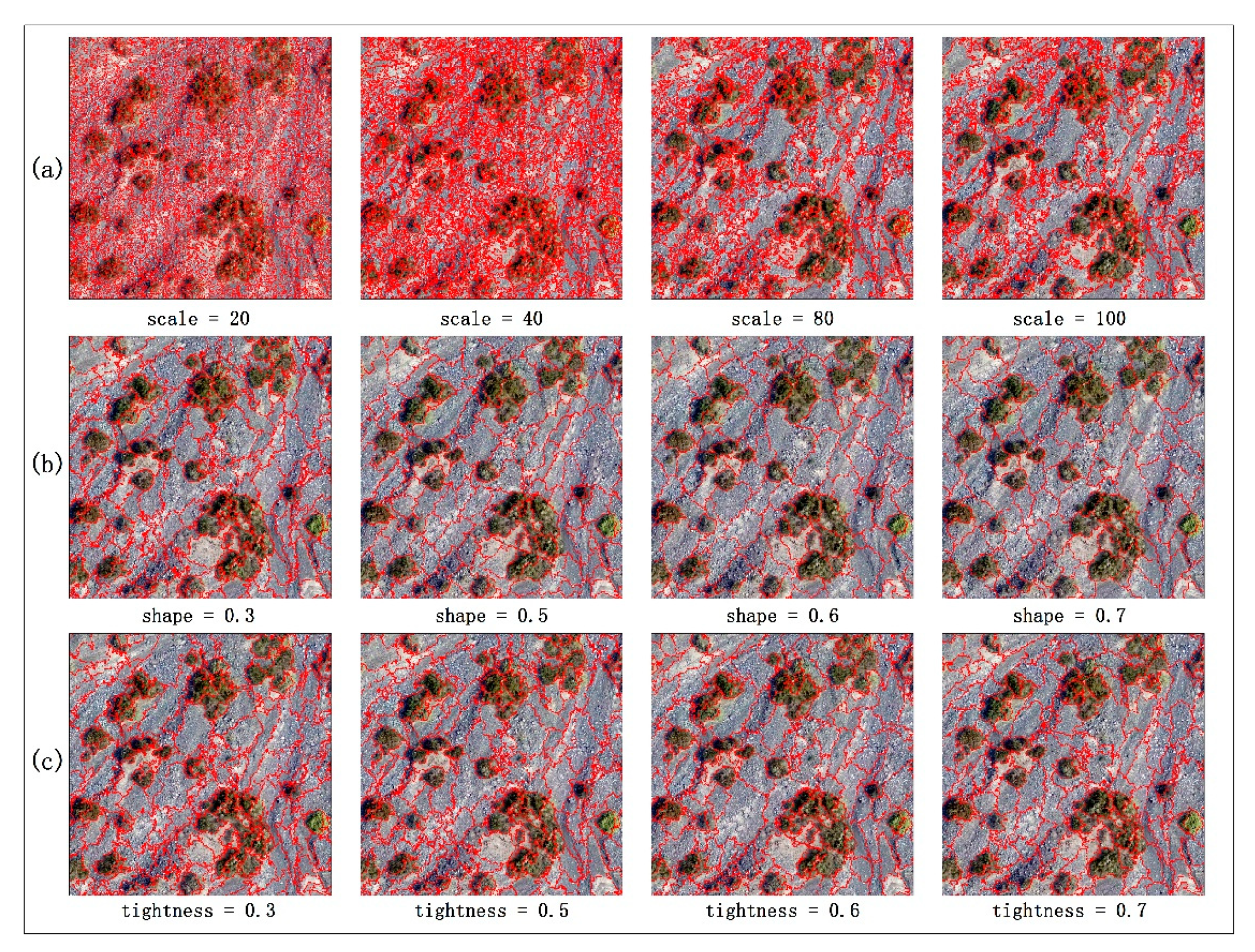
3.1. Image Segmentation Parameter Selection

A combination of different parameters, including scale, shape, and tightness, was examined to select the optimal parameter set for the multi-scale segmentation. In consideration of the image pixel resolution and the canopy widths of the different shrub species, each parameter was tested with four different values used in previous studies. The ranges and intervals of these values were not exactly the same. The ranges of the shape and tightness parameters were both 0.3–0.7. The scale ranged from 20 to 100. The segmentation results for the different parameters are shown in Figure 5. We first tested the scale parameters with the shape and tightness parameters initially set to 0.5. As shown in Figure 5, the segmentation was too scattered at scale parameters of 20 and 50. Under-segmentation occurred when the scale was 100. When the scale was 80, neighboring canopies with similar features were combined into one class.
We then tested the shape and tightness parameters. The scale value was set to the already-determined optimal value of 80, while the tightness parameter was initially set to 0.5. When the shape parameter was 0.3, we obtained a more regular crown shape, which we determined was the optimal value. When the scale and shape were set to 80 and 0.3, respectively, we found that a tightness value of 0.7 yielded a more complete canopy segmentation. Therefore, we set the scale, shape, and tightness parameters to 80, 0.3, and 0.7, respectively, and used the optimal combined parameters of the multi-scale segmentation method. These parameters produced segments with relatively homogeneous spectral and textural features.

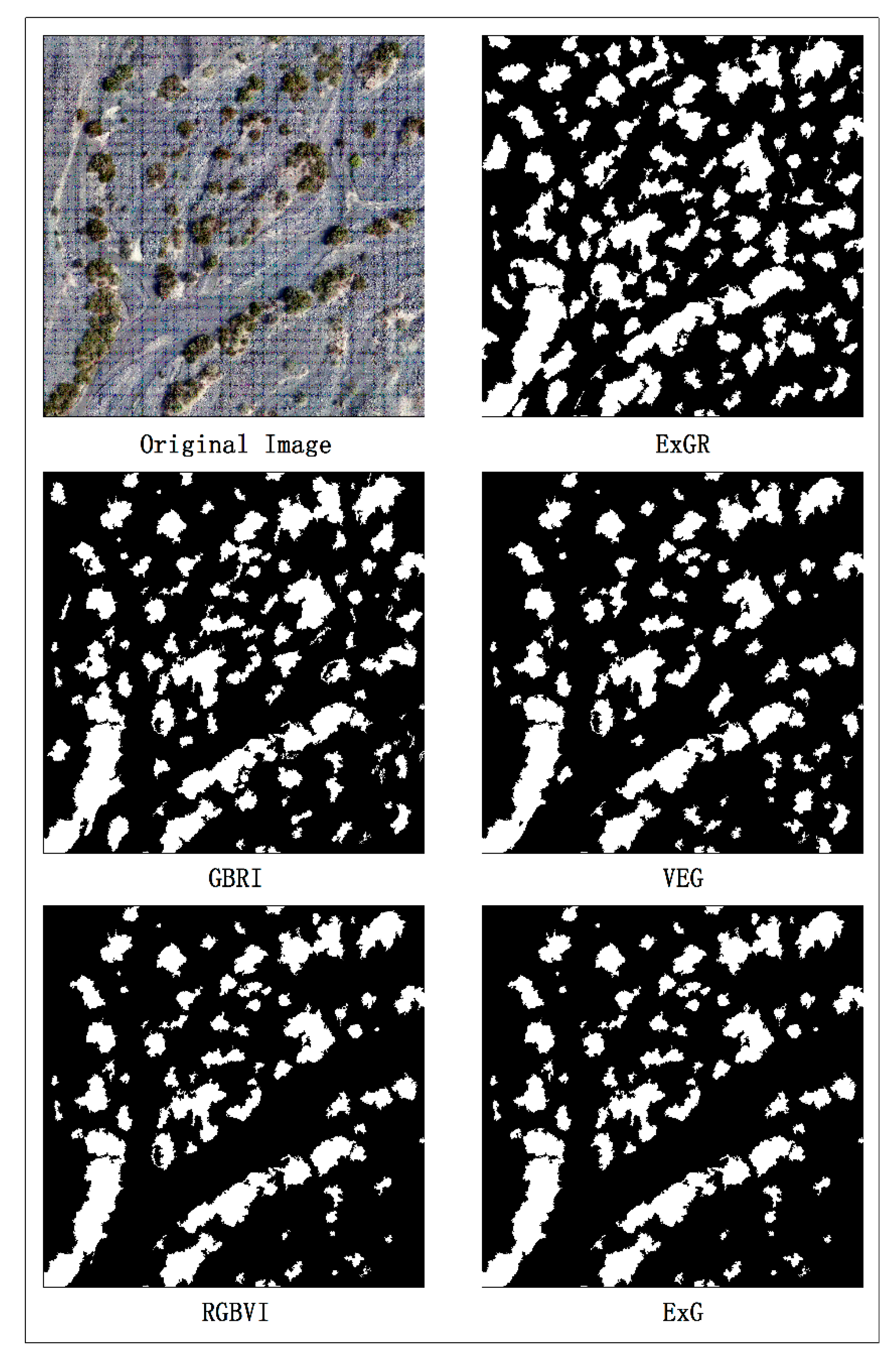
3.2. Classification Results for Vegetation and Non-Vegetation

The threshold values of the five vegetation indices (ExG, ExGR, GBRI, RGBVI, and VEG) were 0.03, −0.11, 1.4, 0.07, and 1.03, respectively. Based on thresholds of different vegetation indices, we obtained the vegetation distribution maps of EXG, ExGR, GBRI, RGBVI, and VEG. A sample of the results is presented in Figure 6, with the vegetation areas and non-vegetation areas shown in white and black, respectively. As is shown in Figure 6, the ExG and RGBVI indices exhibited significant differences from the other indices, in terms of the grey values representing vegetation and non-vegetation areas. The grey values of the vegetation and non-vegetation area were similar for the remaining vegetation indices. The vegetation distribution maps extracted with ExGR and GBRI were very similar, and they both exhibited more misclassifications in the classification process. In most cases, the vegetation commonly exhibited mutual crossovers and overlapped with the non-vegetation area, and the bare soil was commonly mistaken for vegetation. In other words, neither ExGR nor GBRI could discriminate between plants and the background, with the chosen threshold values. The VEG index could distinguish most plants well, but mutual crossovers between some vegetation types and bare soil existed. Therefore, it was clear that ExG and RGBVI were better at separating vegetation from the background in the Gobi region. To better compare the vegetation classification accuracy of different vegetation indices, we classified the vegetation of 38 samples in the Gobi region using each vegetation index. The results shown in Table 2 indicate that ExG performed the best in vegetation classification, with an OA of 0.96 and a maximum Kappa coefficient of 0.93 (Table 2).

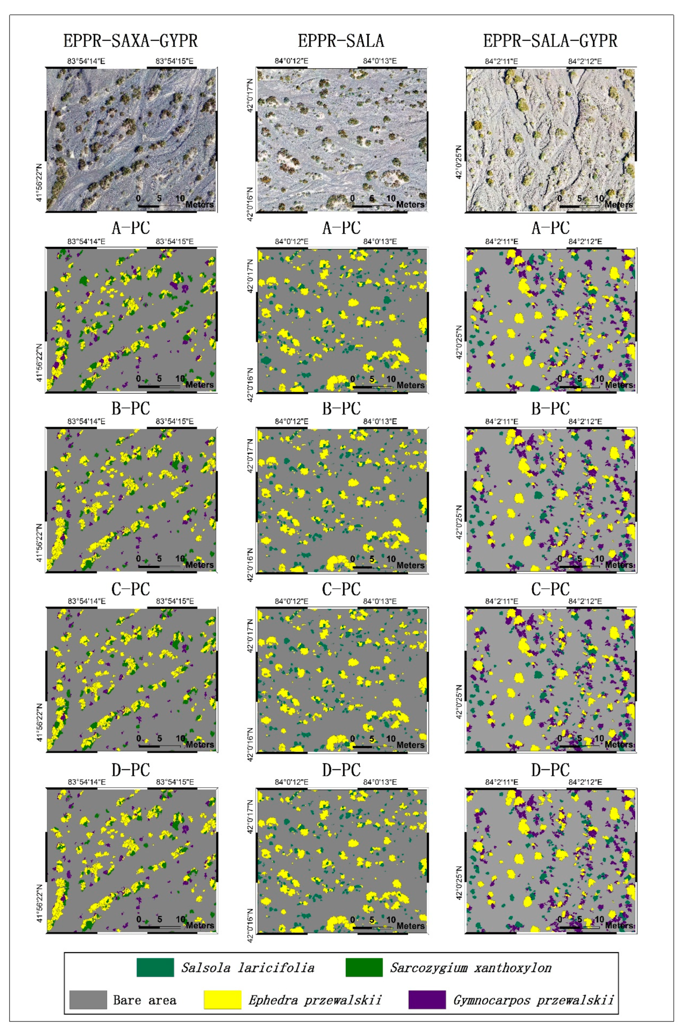
3.3. Classification Results for Individual Shrub Species

PCA produced uncorrelated bands, and the main information was usually contained with the first few components. The important components were selected from all principal components in each type of variable set. Among the four types of variable sets, PC1 and PC2 represented the majority of information, about 94% (Appendix C, Table A4). The first six components with the highest variance were used in each type of variable set, although P3–P6 showed lower information (less than 2.22%, Table A4). All six components were included as the classification input. This was done to reduce the possibility of omissions resulting from the contribution of low-information variables.
Three classifiers were used to classify species from different variable sets. The RF model returned the highest OA (78% on average) and Kappa (0.65 on average), closely followed by the SVM with an average OA and Kappa of 76% and 0.63, respectively. The highest classification accuracy value was produced by a combination of the D-PC variable set and the RF model, with 89% OA and Kappa of 0.82. The results generated by RF and SVM were significantly higher than those generated by k-NN (average OA of 0.62 and average Kappa of 0.50). The evaluations of the three classifiers are presented in Table 3.
Table 4 shows the shrub species classification results generated by a combination of the RF model and four types of variable set (A-PC, B-PC, C-PC, and D-PC). The classification maps for individual shrub species generated by the D-PC variable set (containing a combination of the original bands, all derived spectral indices, and all derived texture indices) had the highest OA, while the classification maps from the A-PC variable set that contained only the original bands had the lowest OA (Table 3 and Table 4). When original bands were combined with all derived spectral indices for shrub species classification, the prediction accuracy was significantly higher, as shown by the B-PC variable set. The combination of original bands and all derived textural indices also improved the prediction accuracy, as shown by the C-PC variable set. However, the classification accuracy produced by the C-PC variable set was slightly lower than that of the B-PC variable set. Moreover, when comparing the UA with the PA, the D-PC variable set generated classification maps with higher accuracies across different categories. Three vegetation alliance types containing at least two shrub species were selected for a more detailed examination of the results, to compare the shrub species classification results in different vegetation alliances. The classification results for each vegetation alliance are shown in Appendix D, Table A5, Table A6 and Table A7.
In each shrub vegetation alliance, the highest classification accuracy was generated by the D-PC variable set, while the lowest classification accuracy was generated by the A-PC variable set. Furthermore, we determined that EPPR–SALA (including two shrub species) had a higher classification accuracy than the other two vegetation alliances. The highest OA and Kappa values obtained based on the best variable set exceeded 94% and 0.89, respectively (Appendix D, Table A6). However, the results of the four variable sets differed greatly between EPPR–SALA–GYPR and EPPR–SAXA–GYPR, especially for B-PC and C-PC. In EPPR–SALA–GYPR, the classification accuracy obtained by the variable set B-PC was higher than that generated by C-PC, while the opposite result was generated in EPPR–SAXA–GYPR (Appendix D, Table A5 and Table A7). The individual shrub species classification maps for the three vegetation alliances, generated by the four types of variable sets, are shown in Figure 7.
When examining the classification success per shrub species, the classification of Ephedra przewalskii was the most accurate since it was the dominant species in all community alliances (Table 4). In EPPR–SAXA–GYPR and EPPR–SALA–GYPR, the classification accuracy of Gymnocarpos przewalskii was low, particularly in EPPR–SALA–GYPR. In addition, the PA and UA of Gymnocarpos przewalskii generated by the optimal variable set (D-PC) were only 0.71 and 0.56, respectively (Appendix D, Table A7), which were far lower than the classification accuracies of the other shrub species. However, the classification accuracy of Gymnocarpos przewalskii generated by D-PC was much higher, as the PA and UA generated by A-PC were 0.29 and 0.24, respectively. In EPPR–SAXA–GYPR, the classification accuracy of Sarcozygium xanthoxylon generated by A-PC was relatively low. However, with the addition of spectral and texture indices as classification variables, the classification accuracy was significantly improved. Its PA and UA increased from 0.43 and 0.5 to 0.68 and 0.77, respectively (Appendix D, Table A5). Moreover, it is worth noting that variable sets C-PC and D-PC produced the same classification accuracy in EPPR–SAXA–GYPR.
In general, whether from the perspective of vegetation alliance type or shrub species category, B-PC (including original bands and all derived spectral indices) and C-PC (including original bands and all derived texture indices) both produced higher accuracies than A-PC, which only used the original band information to classify the shrub species. In contrast, the classification generated by C-PC was slightly less accurate than that of B-PC. The optimal variable set D-PC, which integrates all spectral and textural variables, has the highest classification accuracy, and is more conducive to classifying individual shrub species with different spectral and spatial complexities in the Gobi surface environment.
Table 5 shows statistical results of species types and quantity in 38 sample plots, obtained with a combination of the optimal variable set (D-PC) and RF model. The spatial distributions of species across different regions of the alluvial fans are shown in Figure 8 (Figure 8 shows only three groups of typical plots, representing the top, middle, and bottom of alluvial fans, respectively). Overall, the number of different species was the greatest at the top of the alluvial fan. As the altitude decreased, the type and number of plants decreased significantly. At the bottom of the alluvial fans, only a few Ephedra przewalskii survived. From Figure 8, the spatial distribution of different species on alluvial fans in the Gobi region can be intuitively understood.

4. Discussion

4.1. Use of Multi-Scale Segmentation to Segment UAV Images

Our findings demonstrate the ability to integrate the multi-scale image segmentation algorithm with the RF classification model to estimate individual shrub species in a spatially explicit and consistent way at large scales in the Gobi region. Compared with mapping shrub species based on pixels or by manual measurements during field surveys, the individual shrub-based method developed in this study can directly extract variations between individual shrubs and allows us to combine spectral and structural traits within and between species [76,77]. However, the quality of image segmentation has a major effect on the species classification results. The multi-scale segmentation method is commonly used in high-resolution image segmentation because of its robustness in processing high-resolution images. In this study, the species were sparsely distributed with large gaps between them, so segmentation parameters had varying effects on image segmentation when classifying individual shrub species. By combining the parameters, we found that different parameter combinations (scale, shape, and tightness) yielded varying segmentation results for the UAV images from the Gobi region. The segmentation was too fragmented at smaller scales, while under-segmentation occurred when the scale was too large. Moreover, it was difficult to segment plants with large spectral differences, and adjacent plants with small shape differences were easily incorrectly grouped into the same segment. Therefore, continuous testing is required to determine the most appropriate parameter combination to best separate individual shrubs.

4.2. Individual Shrub-Based Species Classification

Assigning individuals to species using a few remotely sensed features extracted from RGB spectral data is challenging, particularly in the Gobi region where most species are spectrally similar. Even by coalescing both spectral and textural features, only ~89% of all individuals could be correctly assigned to a species (Table 3 and Table 4). However, this level of accuracy was considerable for classification of individual shrub species from only UAV RGB images. In addition, the background (Gobi gravel, sandbags, shadows, etc.) of the Gobi surface has become more complicated due to intense light radiation and erosion by wind and sand throughout the year, making shrub species classification more difficult. The vegetation index can distinguish between vegetation and non-vegetation areas. In this study, we tested the ability of five commonly used vegetation indices to classify vegetation and non-vegetation. The results showed that both ExG and RGBVI could effectively distinguish between vegetation and non-vegetation areas. This has also been verified in many other studies [78,79]. By comparing the vegetation and non-vegetation classification results of the five vegetation indices, we further found that ExG had better vegetation extraction capability than RGBVI in the Gobi region with complex background. This discovery can improve the efficiency of future research on vegetation classification and species classification in the Gobi region.
Four types of variable sets and three classifiers were used for shrub species classification, and PCA was used for feature extraction of each type of variable set. We found that the feature extraction process could provide more reliable and efficient classifications of the variable sets. The first three components of each type of variable set generated by PCA retained most of the information of the different variable sets, which effectively removed redundant variables and significantly improved the classification efficiency. However, in order to balance the computational efficiency and avoid omissions of the contribution for species classification resulting from the low-information variables, the first six components of each variable set were used for the shrub species classification. Of these three classifiers, the RF model produced higher classification accuracy compared with the other two classifiers. However, results of different classifiers showed that the SVM also had a high potential for shrub species classification, although its classification accuracy was slightly lower than RF (Table 3). This was consistent with some previous studies [15,80,81]. In addition, the variable set consisting of the original RGB bands and all the derived spectral and texture indices had more obvious advantages over the others, particularly for some shrub species that were hard to differentiate (e.g., Gymnocarpos przewalskii and Sarcozygium xanthoxylon). Therefore, the variable set selection process was more conducive to classifying these shrub species. Overall, the best variable set combined with the RF model successfully mapped individual shrub species in different vegetation alliances in the Gobi region, with OA and Kappa values of 88.63% and 0.82, respectively.
In the classification process of the three shrub vegetation alliances, the vegetation alliance EPPR–SALA produced higher shrub species classification accuracy than the other two vegetation alliances, indicating that the quantity of shrub species in a shrub vegetation alliance affects the classification accuracy. In general, fewer species will achieve higher classification accuracy, while more species will increase the noise caused by the spectral and textural similarities among the different species, complicating classification and reducing classification accuracy [81]. In addition, as shown in Table 4, the optimal variable set D-PC yielded a higher classification accuracy than the variable set B-PC that only contained the original bands and all derived spectral indices. This may be because textural information helps to distinguish between different species at various scales. This was consistent with the findings of several previous studies. For instance, Tian et al. found that textural measurements could be useful for distinguishing between conifers and broadleaved trees [30], while Cao et al. concluded that textural measurements could help distinguish between tree species with weak spectral differences but large differences in leaf surface structures [55]. Furthermore, the differences between the classification results of the variable sets B-PC and C-PC in the vegetation alliances EPPR–SAXA–GYPR and EPPR–SALA–GYPR showed that both spectral information and texture information could affect the species classification accuracy. Therefore, it was difficult to distinguish shrub species using only spectral information or texture information. The combined use of spectral indices and texture indices helps to classify shrub species accurately in the Gobi region.

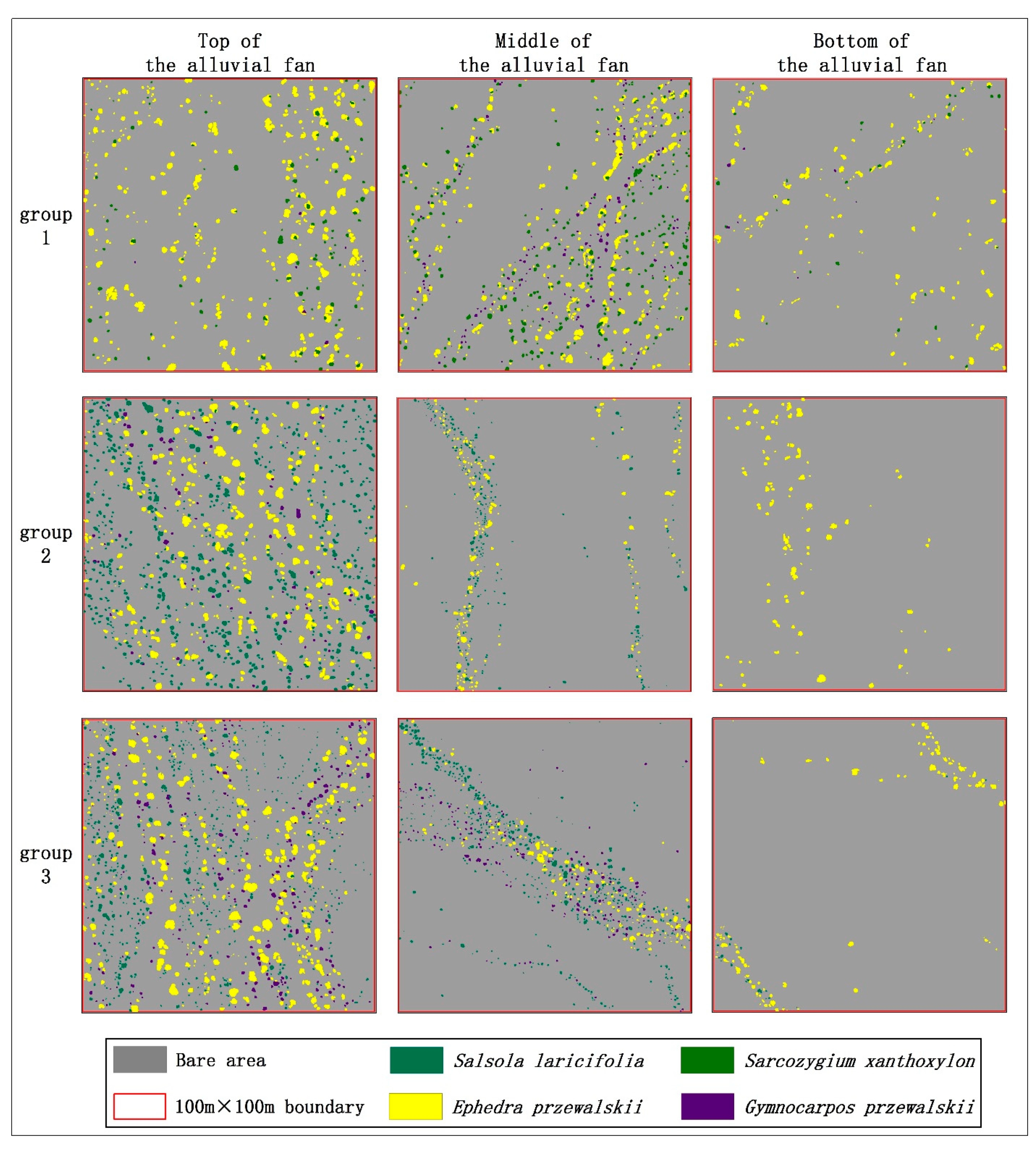
4.3. Spatial Distribution of Vegetation in Different Areas of Alluvial Fans

The species classification results for the 38 sample plots, using the optimal variable set and the RF model, revealed large spatial heterogeneity in the plant composition on the alluvial fan surfaces on the southern slope of the Tian Shan Mountains in the Gobi region. This may be closely correlated with the elevation and the redistribution of water by microtopography. At the top of alluvial fans, due to the flat terrain, the floodwater flowed slowly through the area and stayed on the surface for a long time, resulting in sufficient soil moisture and relatively uniform spatial configuration, which was conducive to the growth of different species. As a result, plants in this region demonstrated a random distribution pattern, with a relatively high number and kinds of plants. The middle and bottom areas of the alluvial fans were more affected by flood erosion and the combined effect of microtopography, forming shallow channels of different sizes. As the floodwater flows through these channels, some of the water seeps into the soil and feeds the plants. As a result, plants in this region were clustered and distributed in channels of varying sizes. In the middle of the alluvial fans, the number of plants was slightly lower than that at the top of the fan due to the limited number of channels, but the kinds of plants are similar. However, at the bottom of alluvial fans, due to the strong evaporation in the Gobi region and the influence of water permeation in the soil surface, the water flow reached this region with a slow speed and a small amount of water, which resulted in limited water supply for plant growth. Therefore, only a small amount of vegetation was distributed in the narrow shallow channel at the bottom of the alluvial fans, and plants of a single type tended to occupy these areas.
As a result of global warming and the drying caused by climate change, local sandstorms were also increasing year by year. In recent years, sandstorms occurred frequently on the edge of the oasis in southern Xinjiang, which seriously threatened the production and lives of people living along the edge of the oasis. The Gobi area in the north of the oasis on the southern slope of the Tian Shan Mountains is closely connected with the oasis, and the vegetation in this area plays an important role in inhibiting the flow of sand on the surface of the Gobi area. A comprehensive understanding of the spatial distribution of different species in the Gobi region is important for ecologists studying the vegetation in this region, including the impact of climate change on vegetation patterns, and for forest managers to take reasonable measures to manage the vegetation in the region. Simultaneously, the spatial distribution of shrub vegetation species on alluvial fans in the Gobi area indirectly reflected the spatial pattern of soil moisture, which provides a basis for afforestation planning in this area.

4.4. Advantages and Limitations

The method developed in this study is not without limitations. One disadvantage is that adequate sample data must be obtainable for a given area to train the RF model. The training data do not need to be spatially uniform, but it can be challenging to obtain sufficient species survey data from individual shrubs in the extremely harsh Gobi environment. Moreover, researchers need to have adequate knowledge of plant taxonomy to accurately distinguish the shrub vegetation species. Furthermore, due to the limitations of the vegetation index, shaded areas, Gobi gravel, or bare ground environments can be misclassified as vegetation if they have similar spectral, textural, and morphological attributes in the vegetation and non-vegetation classification stage. Shrub plants that have similar spectral and textural characteristics to bare ground, such as Gymnocarpos przewalskii and Sarcozygium xanthoxylon, can also be misclassified. This was an issue for the UAV RGB image-based classifications; however, the OBIA re-shaping helped to mitigate misclassifications in a way that cannot be achieved using only the vegetation index. Irregularly shaped objects were excluded using OBIA, or based on their spectral or textural properties. As such, it was possible to automatically segment the UAV images and obtain individual shrub polygons.
In this study, a promising method of image classification was developed and tested. Areas of vegetation were first extracted from UAV images using segmentation and the vegetation index, and then combined with spectral and textural variables within each segment. The optimal variable set was selected and then used with the RF model to classify shrub species. However, the complex surface structure in the Gobi region and the general influence of water limitations on vegetation have resulted in stunted growth and varying plant health. Further development is therefore required before this method can be used to create distribution maps of individual shrub species over large areas without extensive manual editing. Currently, this method is prone to misclassification of shrub species with similar spectral or textural features, such as Gymnocarpos przewalskii and Sarcozygium xanthoxylon. However, these shrub species can also be hard to differentiate from each other without additional data. Besides, the quality of the image segmentation seriously affects the image classification results. The multi-resolution segmentation method we adopted had a good segmentation performance. However, many unsatisfactory segmentation phenomena remain in the complex surface background of the Gobi region, even with an optimized combination of parameters. One possible solution could be using richer spectral data for the different shrub species. For example, multi-spectral or hyperspectral sensors could be carried on a UAV platform [82,83], although this could lead to increased data collection costs. Another solution may be to obtain deeper features from the UAV RGB images for image segmentation and shrub species classification. Deep learning is a recently developed machine learning technology that can mine deep features from data [84,85]. At present, deep learning has been widely used in target detection, image segmentation, image classification, and other fields, and has achieved good results [86,87,88]. The application of deep learning technology to the classification of shrub species in UAV images from the Gobi region is very promising.

5. Conclusions

There are few studies of single shrub species classification based on UAV RGB images in the Gobi region where the surface background is relatively complex. In this work, we proposed a semi-automated workflow to classify individual shrub species based on readily available high-resolution UAV RGB images using a combination of OBIA and RF. We also used PCA to select the best variable sets, and compared the classification accuracies of different classifiers using various sets of variables. We tested this method on different shrub species and vegetation alliances in the Gobi region, and were able to map individual shrub species in all alliances with a mean OA of 88.23% and Kappa of 0.79 using the RF model developed from the best variable set. The PA and UA results for the different shrub species indicate that the classification successfully identified most of the shrub species in each alliance, although the individual shrub species outlines contained false positives that had to be removed manually. In addition, we found that the best detection rates were not necessarily obtained by integrating the derived spectral and textural variables, although the individual shrub species identified were mapped at a higher accuracy using this method than by using only the original spectral bands. The process of feature extraction and variable set selection cannot only improve the running efficiency of the model but can also yield a higher classification accuracy. Some limitations also exist with respect to texturally similar backgrounds such as shading, Gobi gravel, and bare ground that were misclassified as vegetation areas. Nevertheless, the method developed in this study produced promising results, and reduced the amount of manual labor. Based on this method, we obtained and statistically analyzed the species classification results of all sample plots, and obtained the spatial distribution of different species in the study area, which provided further understanding of the composition and spatial distribution of vegetation in the Gobi region. Overall, contributions of this study are as follows: (1) we proposed a combined OBIA and RF model for species classification in the Gobi region based on UAV RGB imagery. (2) We tested the classification accuracy of individual shrub species maps with different types of variable sets generated by different models and confirmed that the combination of spectral and texture indices can significantly improve the species classification accuracy in the Gobi region. (3) By analyzing the species classification results of different locations in the Gobi region on the southern slope of the Tian Shan Mountains, we found that the plant composition of different locations in the Gobi region had greater spatial heterogeneity. Further developments in deep learning methods will hopefully lead to refined identifications of different species spectrums and textures. Therefore, the use of deep learning methods are recommended to identify individual shrub species in future work.

Author Contributions

Conceptualization, Z.L.; formal analysis, Z.L.; funding acquisition, Y.F.; investigation, Z.L., J.D. and H.Z.; methodology, Z.L.; project administration, Y.F.; software, Z.L., J.D. and H.Z.; supervision, Y.F.; validation, Z.L., J.D., H.Z. and Y.F.; visualization, Z.L. and J.D.; writing—original draft, Z.L.; writing—review and editing, Y.F. All authors have read and agreed to the published version of the manuscript.

Funding

This research was funded by the National Natural Science Foundation of China (31770764), the National Key R&D Program (2017YFC0504502), and Fundamental Research Funds for Central Public Welfare Research Institutes (Y2018ZK09).

Institutional Review Board Statement

Not applicable.

Informed Consent Statement

Not applicable.

Acknowledgments

We want to thank Wenke Guan of the XinJiang Academy of Forestry Sciences for supporting our field survey in Luntai, Xinjiang. We sincerely thank the three anonymous reviewers, whose valuable suggestions and comments helped to greatly improve the quality of the article.

Conflicts of Interest

The authors declare that they have no known competing financial interests or personal relationships that could have appeared to influence the work reported in this paper.

Appendix A

Table A1. Description of the selected texture parameters of Gray-Level Co-Occurrence Matrix (GLCM).
TypeVariableDescriptionFormula
Gray-level co-occurrence matrix (GLCM) indicesMeanMean measures the average of gray level values in an image. i = 0 N g 1 j = 0 N g 1 i · g ( i , j )
VarianceMeasures texture heterogeneity. Variance increases when the gray level values differ from their mean. i = 0 N g 1 j = 0 N g 1 ( i μ ) 2 · g ( i , j )
HomogeneityA measure of homogeneity. Sensitive to the presence of near diagonal elements in a GLCM. i = 0 N g 1 j = 0 N g 1 1 1 + ( i j ) 2 · g ( i , j )
ContrastContrast measures the drastic change in gray level between contiguous pixels. Low contrast image features low spatial frequencies. i = 0 N g 1 j = 0 N g 1 ( i j ) 2 · g 2 ( i , j )
DissimilarityDissimilarity is similar to contrast. Instead of weighting the diagonal exponentially, dissimilarity weights increase linearly. i = 0 N g 1 j = 0 N g 1 g ( i , j ) · | i j |
EntropyA measure of the disorder in an image and is highly correlated to energy. Entropy is high when an image is not texturally uniform. i = 0 N g 1 j = 0 N g 1 g 2 ( i , j ) · log ( g ( i , j ) )
EnergyMeasures texture uniformity, or pixel pair repetitions. High energy occurs when the distribution of gray level values is constant or period. i = 0 N g 1 j = 0 N g 1 g 2 ( i , j )
CorrelationMeasures the linear dependency in an image. High correlation values mean a linear relationship between the gray levels of a contiguous set of pixel pairs. i = 0 N g 1 j = 0 N g 1 ( i μ ) · ( j μ ) · g ( i , j ) / σ 2
where Ng is the number of gray levels, g(i,j) is the entry (i,j) in the GLCM, µ is the GLCM mean, and σ2 is the GLCM variance.
Table A2. Formulas of the selected accuracy verification indicators of different classifiers.
NameFormula
Producer’s Accuracy (PA) P P A = X i i X + i
User’s Accuracy (UA) P U A = X i i X i +
Overall Accuracy (OA) P O A = i = 1 n X i i M
Kappa Coefficient (Kappa) K a p p a = M i = 1 n X i i i = 1 n ( X i + · X + i ) M 2 i = 1 n ( X i + · X + i )
where X i i is the amount of correctly classified categories in the error matrix; X + i is the amount of real reference samples in that category; X i + is the number of categories classified into this category; and M is the total amount of samples.

Appendix B

Table A3. The unmanned aerial vehicle (UAV) image data and variables derived from the data.
LayerTypeVariableEquationReference
1Original bandsblue band (B)[13]
2green band (G)
3red band (R)
4Spectral indicesblue green ratio index (BGRI)B/G[64]
5blue ratio (Bratio)B/(B + G + R)[65]
6blue red ratio index (BRRI)B/R[64]
7excess blue index (ExB)1.4 × blue ratio − green ratio[66]
8excess green index (ExG)2 × green ratio − red ratio − blue ratio[66,67]
9excess green red index (ExGR)ExG − ExR[33]
10excess red index (ExR)1.4 × red ratio − green ratio[66]
11green blue ratio index (GBRI)G/B[65]
12green ratio (Gratio)G/(B + G + R)[65]
13green red ratio index (GRRI)G/R[65]
14Kawashima index (IKAW)(R − B)/(R + B)[68]
15color intensity index (INT)(R + G + B)/3[65]
16modified green red vegetation index (MGRVI)(G2 − R2)/(G2 + R2)[69]
17modified VARI (MVARI)(G − B)/(G + R − B)[24]
18normalized green blue difference index (NGBDI)(G − B)/(G + B)[70]
19red blue ratio index (RBRI)R/B[65]
20red green blue vegetation index (RGBVI)(G2 − R × B)/(G2 + R × B)[66]
21red ratio (Rratio)R/(B + G + R)[65]
22triangular greenness index (TGI)G − (0.39 × R) − (0.61 × B)[71]
23visible atmospherically resistant index (VARI)(G − R)/(G + R − B)[24]
24vegetative index (VEG)G/(R0.667 × B0.333)[72]
25visible-band difference vegetation index (VDVI)(G − R − B)/(G + R + B)[24]
26Woebbecke index (WI)(G − B)/(G + R)[67]
27–34Texture indicesB_GLCM (mean, variance, homogeneity, contrast, dissimilarity, entropy, energy, correlation)[45]
35–42G_GLCM (mean, variance, homogeneity, contrast, dissimilarity, entropy, energy, correlation)
43–50R_GLCM (mean, variance, homogeneity, contrast, dissimilarity, entropy, energy, correlation)

Appendix C

Table A4. Percentage of information contained in the first six components of the principal component analysis (PCA) of different sets of variables.
Variable SetPrincipal ComponentsVariance (%)
A-PCPC187.87
PC28.22
PC32.22
PC41.06
PC50.49
PC60.14
B-PCPC185.67
PC28.24
PC32.03
PC41.28
PC50.52
PC60.36
C-PCPC182.03
PC29.92
PC31.76
PC40.74
PC50.31
PC60.25
D-PCPC184.74
PC210.46
PC31.37
PC40.42
PC50.4
PC60.23

Appendix D

Table A5. Comparison of classification accuracies of individual shrub species maps from EPPR–SAXA–GYPR alliance of four sets of variables generated by the random forest (RF) model.
Variable SetClassProducer Accuracy Number
of Samples
Ephedra przewalskiiSarcozygium xanthoxylonGymnocarpos przewalskii
A-PCEphedra przewalskii0.83 176146219
Sarcozygium xanthoxylon0.43 6831298
Gymnocarpos przewalskii0.50 4414822
Total 2881915839
User Accuracy 0.76 0.50 0.56
Overall Accuracy (197/288) = 68.40%Kappa = 0.40
B-PCEphedra przewalskii0.89 176156137
Sarcozygium xanthoxylon0.54 6827374
Gymnocarpos przewalskii0.70 448531
Total 2881915542
User Accuracy 0.82 0.67 0.74
Overall Accuracy (224/288) = 77.78%Kappa = 0.58
C-PCEphedra przewalskii0.92 17616295
Sarcozygium xanthoxylon0.66 6894514
Gymnocarpos przewalskii0.68 4411330
Total 2881726749
User Accuracy 0.94 0.67 0.61
Overall Accuracy (237/288) = 82.29%Kappa = 0.68
D-PCEphedra przewalskii0.92 176162104
Sarcozygium xanthoxylon0.68 6819463
Gymnocarpos przewalskii0.75 447433
Total 2881886040
User Accuracy 0.86 0.77 0.83
Overall Accuracy (237/288) = 82.29%Kappa = 0.68
Table A6. Comparison of classification accuracies of individual shrub species maps from the EPPR–SALA alliance of four sets of variables generated by the random forest (RF) model.
Variable SetClassProducer Accuracy Number
of Samples
Ephedra przewalskiiSalsola laricifolia
A-PCEphedra przewalskii0.70 1379641
Salsola laricifolia0.71 14843105
Total 285139146
User Accuracy 0.69 0.72
Overall Accuracy Kappa = 0.41
(201/285) = 70.53%
B-PCEphedra przewalskii0.80 13710928
Salsola laricifolia0.84 14823125
Total 285132153
User Accuracy 0.83 0.82
Overall Accuracy Kappa = 0.64
(234/285) = 82.11%
C-PCEphedra przewalskii0.74 13710136
Salsola laricifolia0.76 14836112
Total 285137148
User Accuracy 0.74 0.76
Overall Accuracy Kappa = 0.49
(213/285) = 74.74%
D-PCEphedra przewalskii0.92 13712611
Salsola laricifolia0.97 1484144
Total 285130155
User Accuracy 0.97 0.93
Overall Accuracy Kappa = 0.89
(270/285) = 94.74%
Table A7. Comparison of classification accuracies of individual shrub species maps from EPPR–SALA–GYPR alliance of four sets of variables generated by the random forest (RF) model.
Variable SetClassProducer Accuracy Number
of Samples
Ephedra przewalskiiSalsola laricifoliaGymnocarpos przewalskii
A-PCEphedra przewalskii0.73 1441052514
Salsola laricifolia0.74 1462110817
Gymnocarpos przewalskii0.29 3422210
Total 32412815541
User Accuracy 0.82 0.70 0.24
Overall Accuracy
(223/324) = 68.83%
Kappa = 0.48
B-PCEphedra przewalskii0.76 144110268
Salsola laricifolia0.85 1461012412
Gymnocarpos przewalskii0.44 3441515
Total 32412416535
User Accuracy 0.89 0.75 0.43
Overall Accuracy
(249/324) = 76.85%
Kappa = 0.61
C-PCEphedra przewalskii0.64 14492466
Salsola laricifolia0.79 146231167
Gymnocarpos przewalskii0.65 346622
Total 32412116835
User Accuracy 0.76 0.69 0.63
Overall Accuracy
(230/324) = 70.99%
Kappa = 0.51
D-PCEphedra przewalskii0.90 14413059
Salsola laricifolia0.89 146613010
Gymnocarpos przewalskii0.71 341024
Total 32413614543
User Accuracy 0.96 0.90 0.56
Overall Accuracy
(284/324) = 87.65%
Kappa = 0.79

References

  1. Li, X.R. Study on shrub community diversity of Ordos Plateau, Inner Mongolia, Northern China. J. Arid Environ. 2001, 47, 271–279. [Google Scholar]
  2. Hao, H.M.; Huang, Z.; Lu, R.; Jia, C.; Liu, Y.; Liu, B.R.; Wu, G.L. Patches structure succession based on spatial point pattern features in semi-arid ecosystems of the water-wind erosion crisscross region. Glob. Ecol. Conserv. 2017, 12, 158–165. [Google Scholar] [CrossRef]
  3. Halle, H.W.; Göttingen, K.W.; Marburg, G.M. Plant communities of the southern Mongolian Gobi. Phytocoenologia 2009, 39, 331–376. [Google Scholar]
  4. Li, F.R.; Liu, J.L.; Liu, C.A.; Niu, R.X. Shrubs and species identity effects on the distribution and diversity of ground-dwelling arthropods in a Gobi desert. J. Insect Conserv. 2013, 17, 319–331. [Google Scholar] [CrossRef]
  5. Guo, Z.C.; Wang, T.; Liu, S.L.; Kang, W.P.; Chen, X.; Feng, K.; Zhang, X.Q.; Zhi, Y. Biomass and vegetation coverage survey in the Mu Us sandy land-based on unmanned aerial vehicle RGB images. Int. J. Appl. Earth Obs. Geoinf. 2021, 94, 102239. [Google Scholar] [CrossRef]
  6. Ripley, B.D. Modeling spatial patterns. J. R. Stat. Soc. 1977, 39, 172–212. [Google Scholar]
  7. Huang, H.Y.; Li, X.; Chen, C.C. Individual tree crown detection and delineation from very-high-Resolution UAV images based on Bias field and marker-controlled watershed segmentation algorithms. IEEE J. Sel. Top. Appl. Earth Obs. Remote Sens. 2018, 11, 2253–2262. [Google Scholar] [CrossRef]
  8. Chang, Y.M.; Baddeley, A.; Wallace, J.; Canci, M. Spatial statistical analysis of tree deaths using airborne digital imagery. Int. J. Appl. Earth Obs. Geoinf. 2013, 21, 418–426. [Google Scholar] [CrossRef]
  9. Salovaara, K.J.; Thessler, S.; Malik, R.N.; Tuomisto, H. Classification of Amazonian primary rain forest vegetation using Landsat ETM+ satellite imagery. Remote Sens. Environ. 2005, 97, 39–51. [Google Scholar] [CrossRef]
  10. Pant, P.; Heikkinen, V.; Hovi, I.A.; Korpela, I.; Hauta-Kasari, M.; Tokola, T. Evaluation of simulated bands in airborne optical sensors for tree species identification. Remote Sens. Environ. 2013, 138, 27–37. [Google Scholar] [CrossRef]
  11. Fassnacht, F.; Latifi, H.; Stereńczak, K.; Modzelewska, A.; Lefsky, M.; Waser, L.; Ghosh, A. Review of studies on tree species classification from remotely sensed data. Remote Sens. Environ. 2016, 186, 64–87. [Google Scholar] [CrossRef]
  12. Ozdarici-Ok, A. Automatic detection and delineation of citrus trees from VHR satellite imagery. Int. J. Remote Sens. 2015, 36, 4275–4296. [Google Scholar] [CrossRef]
  13. Zhang, X.L.; Zhang, F.; Qi, Y.X.; Deng, L.F.; Wang, X.L.; Yang, S.T. New research methods for vegetation information extraction based on visible light remote sensing images from an unmanned aerial vehicle (UAV). Int. J. Appl. Earth Obs. Geoinf. 2019, 78, 215–226. [Google Scholar] [CrossRef]
  14. Picos, J.; Bastos, G.; Míguez, D.; Alonso, L.; Armesto, J. Individual tree detection in a eucalyptus plantation using unmanned aerial vehicle (UAV)-LiDAR. Remote Sens. 2020, 12, 885. [Google Scholar] [CrossRef] [Green Version]
  15. Onishi, M.; Ise, T. Explainable identification and mapping of trees using UAV RGB image and deep learning. Sci. Rep. 2021, 11, 903. [Google Scholar] [CrossRef]
  16. Marcial-Pablo, M.d.J.; Gonzalez-Sanchez, A.; Jimenez-Jimenez, S.I.; Ontiveros-Capurata, R.E.; Ojeda-Bustamante, W. Estimation of vegetation fraction using RGB and multispectral images from UAV. Int. J. Remote Sens. 2019, 40, 420–438. [Google Scholar] [CrossRef]
  17. Riaño, D.; Chuvieco, E.; Condés, S.; González-Matesanz, J.; Ustin, S.L. Generation of crown bulk density for Pinus sylvestris L. From lidar. Remote Sens. Environ. 2004, 92, 345–352. [Google Scholar] [CrossRef]
  18. Suratno, A.; Seielstad, C.; Queen, L. Tree species identification in mixed coniferous forest using airborne laser scanning. ISPRS J. Photogramm. Remote Sens. 2009, 64, 683–693. [Google Scholar] [CrossRef]
  19. Korpela, I.; Ørka, H.O.; Hyyppä, J.; Heikkinen, V.; Tokola, T. Range and AGC normalization in airborne discrete-return LiDAR intensity data for forest canopies. ISPRS J. Photogramm. Remote Sens. 2010, 65, 369–379. [Google Scholar] [CrossRef]
  20. Zhang, K.W.; Hu, B.X. Individual urban tree species classification using very high spatial resolution airborne multi-spectral imagery using longitudinal profiles. Remote Sens. 2012, 4, 1741–1757. [Google Scholar] [CrossRef] [Green Version]
  21. Franklin, S.E. Pixel- and object-based multispectral classification of forest tree species from small unmanned aerial vehicles. J. Unmanned Veh. Syst. 2018, 6, 195–211. [Google Scholar] [CrossRef] [Green Version]
  22. Koc-San, D.; Selim, S.; Aslan, N.; San, B.T. Automatic citrus tree extraction from UAV images and digital surface models using circular Hough transform. Comput. Electron. Agric. 2018, 150, 289–301. [Google Scholar] [CrossRef]
  23. Iizuka, K.; Yonehara, T.; Itoh, M.; Kosugi, Y. Estimating tree height and diameter at breast height (DBH) from digital surface models and orthophotos obtained with an unmanned aerial system for a Japanese Cypress (Chamaecyparis obtusa) Forest. Remote Sens. 2018, 10, 13. [Google Scholar] [CrossRef] [Green Version]
  24. Cen, H.Y.; Wan, L.; Zhu, J.P.; Li, Y.J.; Li, X.R.; Zhu, Y.M.; Weng, H.Y.; Wu, W.K.; Yin, W.X.; Xu, C.; et al. Dynamic monitoring of biomass of rice under different nitrogen treatments using a lightweight UAV with dual image-frame snapshot cameras. Plant Methods 2019, 15, 32. [Google Scholar] [CrossRef] [PubMed]
  25. Karimi, Y.; Prasher, S.O.; Patel, R.M.; Kim, S.H. Application of support vector machine technology for weed and nitrogen stress detection in corn. Comput. Electron. Agric. 2006, 51, 99–109. [Google Scholar] [CrossRef]
  26. Safonova, A.; Tabik, S.; Alcaraz-Segura, D.; Rubtsov, A.; Maglinets, Y.; Herrera, F. Detection of Fir Trees (Abies sibirica) Damaged by the Bark Beetle in Unmanned Aerial Vehicle Images with Deep Learning. Remote Sens. 2019, 11, 643. [Google Scholar] [CrossRef] [Green Version]
  27. Weinstein, B.G.; Marconi, S.; Bohlman, S.A.; Zare, A.; White, E.P. Cross-site learning in deep learning RGB tree crown detection. Ecol. Inform. 2020, 56, 101061. [Google Scholar] [CrossRef]
  28. Nevalainen, O.; Honkavaara, E.; Tuominen, S.; Viljanen, N.; Hakala, T.; Yu, X.; Hyyppä, J.; Saari, H.; Pölönen, I.; Imai, N.N.; et al. Individual tree detection and classification with UAV-Based photogrammetric point clouds and hyperspectral imaging. Remote Sens. 2017, 9, 185. [Google Scholar] [CrossRef] [Green Version]
  29. Breiman, L. Random forests. Mach. Learn. 2001, 45, 5–32. [Google Scholar] [CrossRef] [Green Version]
  30. Räsänen, A.; Juutinen, S.; Tuittila, E.; Aurela, M.; Virtanen, T. Comparing ultra-high spatial resolution remote-sensing methods in mapping peatland vegetation. J. Veg. Sci. 2019, 30, 1016–1026. [Google Scholar] [CrossRef]
  31. Sheykhmousa, M.; Mahdianpari, M.; Ghanbari, H.; Mohammadimanesh, F.; Ghamisi, P.; Homayouni, S. Support Vector Machine versus Random Forest for Remote Sensing Image Classification: A Meta-Analysis and Syst-ematic Review. IEEE J. Sel. Top. Appl. Earth Obs. Remote Sens. 2020, 13, 6308–6325. [Google Scholar] [CrossRef]
  32. Talukdar, S.; Singha, P.; Mahato, S.; Shahfahad; Pal, S.; Liou, Y.-A.; Rahman, A. Land-Use Land-Cover Classification by Machine Learning Classifiers for Satellite Observations—A Review. Remote Sens. 2020, 12, 1135. [Google Scholar] [CrossRef] [Green Version]
  33. Niederheiser, R.; Rutzinger, M.; Bremer, M.; Wichmann, V. Dense image matching of terrestrial imagery for deriving high-resolution topographic properties of vegetation locations in alpine terrain. Int. J. Appl. Earth Obs. Geoinf. 2018, 66, 146–158. [Google Scholar] [CrossRef]
  34. Tian, X.M.; Chen, L.; Zhang, X.L. Classifying tree species in the plantations of southern China based on wavelet analysis and mathematical morphology. Comput. Geosci. 2021, 151, 104757. [Google Scholar] [CrossRef]
  35. Zhao, C.H.; Gao, B.; Zhang, L.J.; Wan, X.Q. Classification of Hyperspectral Imagery based on spectral gradient, SVM and spatial random forest. Infrared Phys. Technol. 2018, 95, 61–69. [Google Scholar]
  36. Xu, J.; Gu, H.B.; Meng, Q.M.; Cheng, J.H.; Liu, Y.H.; Jiang, P.A.; Sheng, J.D.; Deng, J.; Bai, X. Spatial pattern analysis of Haloxylon ammodendron using UAV imagery—A case study in the Gurbantunggut Desert. Int. J. Appl. Earth Obs. Geoinf. 2019, 83, 101891. [Google Scholar] [CrossRef]
  37. Mellor, A.; Haywood, A.; Stone, C.; Jones, S. The Performance of Random Forests in an Operational Setting for Large Area Sclerophyll Forest Classification. Remote Sens. 2013, 5, 2838–2856. [Google Scholar] [CrossRef] [Green Version]
  38. Alvarez-Taboada, F.; Paredes, C.; Julián-Pelaz, J. Mapping of the invasive species Hakea sericea using Unmanned Aerial Vehicle (UAV) and WorldView-2 imagery and an object-oriented approach. Remote Sens. 2017, 9, 913. [Google Scholar] [CrossRef] [Green Version]
  39. Mallinis, G.; Koutsias, N.; Tsakiri-Strati, M.; Karteris, M. Object-based classification using Quickbird imagery for delineating forest vegetation polygons in a Mediterranean test site. ISPRS J. Photogramm. Remote Sens. 2008, 63, 237–250. [Google Scholar] [CrossRef]
  40. Salamí, E.; Barrado, C.; Pastor, E. UAV Flight Experiments Applied to the Remote Sensing of Vegetated Areas. Remote Sens. 2014, 6, 11051–11081. [Google Scholar] [CrossRef] [Green Version]
  41. Gebreslasie, M.T.; Ahmed, F.B.; van Aardt, J.A.N. Extracting structural attributes from IKONOS imagery for Eucalyptus plantation forests in KwaZulu-Natal, South Africa, using image texture analysis and artificial neural networks. Int. J. Remote Sens. 2011, 32, 7677–7701. [Google Scholar] [CrossRef]
  42. Charoenjit, K.; Zuddas, P.; Allemand, P.; Pattanakiat, S.; Pachana, K. Estimation of biomass and carbon stock in Para rubber plantations using object-based classification from Thaichote satellite data in Eastern Thailand. J. Appl. Remote Sens. 2015, 9, 096072. [Google Scholar] [CrossRef] [Green Version]
  43. Herold, M.; Liu, X.H.; Clarke, K.C. Spatial Metrics and Image Texture for Mapping Urban Land Use. Photogramm. Eng. Remote Sens. 2003, 11, 991–1001. [Google Scholar] [CrossRef] [Green Version]
  44. Wood, E.M.; Pidgeon, A.M.; Radeloff, V.C.; Keuler, N.S. Image texture as a remotely sensed measure of vegetation structure. Remote Sens. Environ. 2012, 121, 516–526. [Google Scholar] [CrossRef]
  45. Park, Y.; Guldmann, J.M. Measuring continuous landscape patterns with Gray-Level Co-Occurrence Matrix (GLCM) indices: An alternative to patch metrics? Ecol. Indic. 2020, 109, 105802. [Google Scholar] [CrossRef]
  46. Zhang, F.; Yang, X.J. Improving land cover classification in an urbanized coastal area by random forests: The role of variable selection. Remote Sens. Environ. 2020, 251, 112105. [Google Scholar] [CrossRef]
  47. Simonetti, E.; Simonetti, D.; Preatoni, D. Phenology-Based Land Cover Classification Using Landsat 8 Time Series; European Commission Joint Research Center: Ispra, Italy, 2014. [Google Scholar]
  48. Wicaksono, P. Improving the accuracy of Multispectral-based benthic habitats mapping using image rotations: The application of Principle Component Analysis and Independent Component Analysis. Eur. J. Remote Sens. 2016, 49, 433–463. [Google Scholar] [CrossRef] [Green Version]
  49. Herkül, K.; Kotta, J.; Kutser, T.; Vahtmäe, E. Relating Remotely Sensed Optical Variability to Marine Benthic Biodiversity. PLoS ONE. 2013, 8, e55624. [Google Scholar] [CrossRef] [PubMed] [Green Version]
  50. Pu, R.L.; Liu, D.S. Segmented canonical discriminant analysis of in situ hyperspectral data for identifying 13 urban tree species. Int. J. Remote Sens. 2011, 32, 2207–2226. [Google Scholar] [CrossRef]
  51. Immitzer, M.; Atzberger, C.; Koukal, T. Tree species classification with random Forest using very high spatial resolution 8-Band WorldView-2 satellite data. Remote Sens. 2012, 4, 2661–2693. [Google Scholar] [CrossRef] [Green Version]
  52. Ke, Y.; Quackenbush, L.J.; Im, J. Synergistic use of QuickBird multispectral imagery and LIDAR data for object-based forest species classification. Remote Sens. Environ. 2010, 114, 1141–1154. [Google Scholar] [CrossRef]
  53. Brandt, M.; Tucker, C.J.; Kariryaa, A.; Rasmussen, K.; Abel, C.; Small, J.; Chave, J.; Rasmussen, L.V.; Hiernaux, P.; Diouf, A.A.; et al. An unexpectedly large count of trees in the West African Sahara and Sahel. Nature. 2020, 587, 78–82. [Google Scholar] [CrossRef] [PubMed]
  54. Blaschke, T.; Hay, G.J.; Kelly, M.; Lang, S.; Hofmann, P.; Addink, E.; Tiede, D. Geographic Object-Based Image Analysis—Towards a new paradigm. ISPRS Int. J. Geo-Inf. 2014, 87, 180–191. [Google Scholar] [CrossRef] [PubMed] [Green Version]
  55. Cao, J.J.; Leng, W.C.; Liu, K.; Liu, L.; He, Z.; Zhu, Y.H. Object-based mangrove species classification using unmanned aerial vehicle hyperspectral images and digital surface models. Remote Sens. 2018, 10, 89. [Google Scholar] [CrossRef] [Green Version]
  56. Robson, B.A.; Bolch, T.; MacDonell, S.; Hölbling, D.; Rastner, P.; Schaffer, N. Automated detection of rock glaciers using deep learning and object-based image analysis. Remote Sens. Environ. 2020, 250, 112033. [Google Scholar] [CrossRef]
  57. Tang, Y.W.; Jing, L.H.; Li, H.; Atkinson, P.M. A multiple-point spatially weighted k-NN method for object-based classification. Int. J. Appl. Earth Obs. Geoinf. 2016, 52, 263–274. [Google Scholar] [CrossRef] [Green Version]
  58. Machala, M.; Zejdová, L. Forest mapping through object-based image analysis of multispectral and LiDAR aerial data. Eur. J. Remote Sens. 2014, 47, 117–131. [Google Scholar] [CrossRef]
  59. Korznikov, K.A.; Kislov, D.E.; Altman, J.; Doležal, J.; Vozmishcheva, A.S.; Krestov, P.V. Using U-Net-Like Deep Convolutional Neural Networks for Precise Tree Recognition in Very High Resolution RGB (Red, Green, Blue) Satellite Images. Forests. 2021, 12, 66. [Google Scholar] [CrossRef]
  60. Ma, L.; Li, M.; Ma, X.; Cheng, L.; Du, P.; Liu, Y. A review of supervised object-based land-cover image classification. ISPRS J. Photogramm. Remote Sens. 2017, 130, 277–293. [Google Scholar] [CrossRef]
  61. Blaschke, T. Object based image analysis for remote sensing. ISPRS J. Photogramm. 2010, 65, 2–16. [Google Scholar] [CrossRef] [Green Version]
  62. Hossain, M.D.; Chen, D. Segmentation for object-based image analysis (OBIA): A review of algorithms and challenges fromremote sensing perspective. ISPRS J. Photogramm. 2019, 150, 115–134. [Google Scholar] [CrossRef]
  63. Johnson, B.A.; Ma, L. Image Segmentation and Object-Based Image Analysis for Environmental Monitoring: Recent Areas of Interest, Researchers’ Views on the Future Priorities. Remote Sens. 2020, 12, 1772. [Google Scholar] [CrossRef]
  64. Yue, J.B.; Feng, H.K.; Jin, X.L.; Yuan, H.H.; Li, Z.H.; Zhou, C.Q.; Yang, G.J.; Tian, Q.J. A Comparison of Crop Parameters Estimation Using Images from UAV-Mounted Snapshot Hyperspectral Sensor and High-Definition Digital Camera. Remote Sens. 2018, 10, 1138. [Google Scholar] [CrossRef] [Green Version]
  65. Maimaitijiang, M.; Sagan, V.; Sidike, P.; Maimaitiyiming, M.; Hartling, S.; Peterson, K.T.; Maw, M.J.W.; Shakoor, N.; Mockler, T.; Fritschi, F.B. Vegetation Index Weighted Canopy Volume Model (CVMVI) for soybean biomass estimation from Unmanned Aerial System-based RGB imagery. ISPRS J. Photogramm. Remote Sens. 2019, 151, 27–41. [Google Scholar] [CrossRef]
  66. Bendig, J.; Yu, K.; Aasen, H.; Bolten, A.; Bennertz, S.; Broscheit, J.; Gnypabc, M.L.; Barethac, G. Combining uav-based plant height from crop surface models, visible, and near infrared vegetation indices for biomass monitoring in barley. Int. J. Appl. Earth Obs. Geoinf. 2015, 39, 79–87. [Google Scholar] [CrossRef]
  67. Woebbecke, D.M.; Meyer, G.E.; Bargen, K.V.; Mortensenet, D.A. Color Indices for Weed Identification under Various Soil, Residue, and Lighting Conditions. Trans. ASAE 1995, 38, 259–269. [Google Scholar] [CrossRef]
  68. Kawashima, S.; Nakatani, M. An algorithm for estimating chlorophyll content in leaves using a video camera. Ann. Bot. 1998, 81, 49–54. [Google Scholar] [CrossRef] [Green Version]
  69. Nie, S.; Wang, C.; Dong, P.; Xi, X.; Zhou, H. Estimating leaf area index of maize using airborne discrete-return lidar data. IEEE J. Sel. Top. Appl. Earth Obs. Remote Sens. 2016, 9, 3259–3266. [Google Scholar] [CrossRef]
  70. Hunt, E.R.; Cavigelli, M.; Daughtry, C.S.T.; Mcmurtrey, J.E.; Walthall, C.L. Evaluation of digital photography from model aircraft for remote sensing of crop biomass and nitrogen status. Precis. Agric. 2005, 6, 359–378. [Google Scholar] [CrossRef]
  71. Hunt, E.R.; Daughtry, C.S.T.; Mirsky, S.B.; Hively, W.D. Remote sensing with simulated unmanned aircraft imagery for precision agriculture applications. IEEE J. Sel. Top. Appl. Earth Obs. Remote Sens. 2014, 7, 4566–4571. [Google Scholar] [CrossRef]
  72. Hague, T.; Tillett, N.D.; Wheeler, H. Automated crop and weed monitoring in widely spaced cereals. Precis. Agric. 2006, 7, 21–32. [Google Scholar] [CrossRef]
  73. Niazmardi, S.; Homayouni, S.; Safari, A.; Mc, H.; Shang, J.L.; Beckett, K. Histogram-based spatio-temporal feature classification of vegetation indices time-series for crop mapping. Int. J. Appl. Earth Obs. Geoinf. 2018, 72, 34–41. [Google Scholar] [CrossRef]
  74. Kuhn, M. Building Predictive Models in R Using the caret Package. J. Stat. Softw. 2008, 28, 1–26. [Google Scholar] [CrossRef] [Green Version]
  75. Jimenez-Berni, J.A.; Deery, D.M.; Rozas-Larraondo, P.; Condon, A.G.; Rebetzke, G.J.; James, R.A.; Bovill, W.D.; Furbank, R.T.; Sirault, X.R.R. High throughput determination of plant height, ground cover, and above-ground biomass in Wheat with LiDAR. Front. Plant Sci. 2018, 9, 237. [Google Scholar] [CrossRef] [PubMed] [Green Version]
  76. Jing, L.H.; Hu, B.X.; Noland, T.; Li, J.L. An individual tree crown delineation method based on multi-scale segmentation of imagery. J. Photogramm. Remote Sens. 2012, 70, 88–98. [Google Scholar] [CrossRef]
  77. Wang, H.Y.; Shen, Z.F.; Zhang, Z.H.; Xu, Z.Y.; Li, S.; Jiao, S.H.; Lei, Y.T. Improvement of Region-Merging Image Segmentation Accuracy Using Multiple Merging Criteria. Remote Sens. 2021, 13, 2782. [Google Scholar] [CrossRef]
  78. Han, L.; Yang, G.J.; Dai, H.Y.; Xu, B.; Yang, H.; Feng, H.K.; Li, Z.H.; Yang, X.D. Modeling maize above-ground biomass based on machine learning approaches using UAV remote-sensing data. Plant Methods. 2019, 15, 1–19. [Google Scholar] [CrossRef] [PubMed] [Green Version]
  79. Liu, Y.N.; Liu, S.S.; Li, J.; Guo, X.Y.; Wang, S.Q.; Lu, J.W. Estimating biomass of winter oilseed rape using vegetation indices and texture metrics derived from UAV multispectral images. Comput. Electron. Agric. 2019, 166, 105026. [Google Scholar] [CrossRef]
  80. Yan, S.; Yao, X.C.; Zhu, D.H.; Liu, D.Y.; Zhang, L.; Yu, G.J.; Gao, B.B.; Yang, J.Y.; Yun, W.J. Large-scale crop mapping from multi-source optical satellite imageries using machine learning with discrete grids. Int. J. Appl. Earth Obs. 2021, 103, 102485. [Google Scholar] [CrossRef]
  81. Casapia, X.T.; Falen, L.; Bartholomeus, H.; Cárdenas, R.; Flores, G.; Herold, M.; Coronado, E.N.H.; Baker, T.R. Identifying and Quantifying the Abundance of Economically Important Palms in Tropical Moist Forest Using UAV Imagery. Remote Sens. 2019, 12, 9. [Google Scholar] [CrossRef] [Green Version]
  82. Peerbhay, K.Y.; Mutanga, O.; Ismail, R. Investigating the capability of few strategically placed worldview-2 multispectral bands to discriminate Forest species in KwaZulu-Natal, South Africa. IEEE J. Sel. Top. Appl. Earth Obs. Remote Sens. 2014, 7, 307–316. [Google Scholar] [CrossRef]
  83. Li, Y.S.; Li, Q.T.; Liu, Y.; Xie, W.X. A spatial-spectral SIFT for hyperspectral image matching and classification. Pattern Recogn. Lett. 2019, 127, 18–26. [Google Scholar] [CrossRef]
  84. Ise, T.; Minagawa, M.; Onishi, M. Identifying 3 moss species by deep learning, using the “chopped picture” method. Open J. Ecol. 2018, 8, 166–173. [Google Scholar] [CrossRef] [Green Version]
  85. Reichstein, M.; Camps-Valls, G.; Stevens, B.; Jung, M.; Denzler, J.; Carvalhais, N. Deep learning and process understanding for data-driven Earth system science. Nature 2019, 566, 195–204. [Google Scholar] [CrossRef] [PubMed]
  86. Ma, L.; Liu, Y.; Zhang, X.; Ye, Y.; Yin, G.; Johnson, B.A. Deep learning in remote sensing applications: A meta-analysis and review. ISPRS J. Photogramm. Remote Sens. 2019, 152, 166–177. [Google Scholar] [CrossRef]
  87. Minaee, S.; Boykov, Y.Y.; Porikli, F.; Plaza, A.J.; Kehtarnavaz, N.; Terzopoulos, D. Image Segmentation Using Deep Learning: A Survey. IEEE Trans. Pattern Anal. Mach. Intell. 2021. [Google Scholar] [CrossRef]
  88. Muhammad, Z.K.; Mohan, K.G.; Yugyung, L.; Muazzam, A.K. Deep Neural Architectures for Medical Image Semantic Segmentation: Review. Access IEEE 2021, 9, 83002–83024. [Google Scholar]
Figure 1. Location of the study area (yellow rectangle) in the Gobi region. The backdrop is a Landsat-8 satellite image.
Remotesensing 13 04995 g001
Figure 2. Unmanned aerial vehicle (UAV) images processing of shrub vegetation alliances used for shrub species classification experiments and the sampling plots within the study area.
Remotesensing 13 04995 g002
Figure 3. Ground-based photos of different shrub species (ad) and their corresponding unmanned aerial vehicle (UAV) images (eh).
Remotesensing 13 04995 g003
Figure 4. Workflow for classification of individual shrub species. Abbreviations used in the classification step: excess green red index (ExGR), green blue ratio index (GBRI), vegetative index (VEG), red green blue vegetation index (RGBVI), excess green index (ExG), k-nearest neighbors (k-NN), support vector machine (SVM), random forest (RF), principal component analysis (PCA). The A-PC, B-PC, C-PC, and D-PC represent the sets of variables used in the classification experiments of shrub species after principal component analysis (PCA) of layers A, B, C, and D, respectively.
Remotesensing 13 04995 g004
Figure 5. Example of the multi-scale segmentation results with various scale, shape, and tightness parameters. (a) Segmentation results of various scales (shape = 0.5, tightness = 0.5). (b) Segmentation results of various shapes (scale = 80, tightness = 0.5). (c) Segmentation results of various tightness parameters (scale = 80, shape = 0.3).
Remotesensing 13 04995 g005
Figure 6. Results of extraction using different vegetation indices in the Gobi region (30 × 30 m). The white color is vegetation area, and black is non-vegetation area. Abbreviations: excess green red index (ExGR), green blue ratio index (GBRI), vegetative index (VEG), red green blue vegetation index (RGBVI), excess green index (ExG).
Remotesensing 13 04995 g006
Figure 7. Unmanned aerial vehicle (UAV) RGB image of the three shrub vegetation alliances (EPPR–SAXA–GYPR; EPPR–SALA; and EPPR–SALA–GYPR) and the corresponding prediction results for the four sets of variables (A-PC, B-PC, C-PC, and D-PC) generated by the random forest (RF) model.
Remotesensing 13 04995 g007
Figure 8. Spatial distribution of shrub species across different areas (top, middle, and bottom) of alluvial fans.
Remotesensing 13 04995 g008
Table 1. The shrub species classification category adopted and the number of training and testing samples.
ClassDescriptionTraining
(Number of Segments)
Testing
(Number of Segments)
Ephedra przewalskiiThe corresponding average height and crown width are 0.41 and 1 m. Growth between individual plants greatly differed. In UAV images, the individual shrub mostly appears yellowish green.1067457
Salsola laricifoliaThe average height is 0.25 m, and the average crown width is 0.49 m. It is often associated with individual Ephedra przewalskii plant. In UAV images, the individual shrub mostly appears dark green.686294
Sarcozygium xanthoxylonShrub vegetation with fewer leaves and more thick branches. The average height is 0.47 m, and the average crown width is 0.83 m. In UAV images, the individual shrub mostly appears light green.15968
Gymnocarpos przewalskiiShrub vegetation with fewer leaves and more twigs. The average height is 0.34 m, the average crown width is 0.64 m, and the number of Gymnocarpos przewalskii is less. In UAV images, the individual shrub mostly appears light green.18278
Table 2. Accuracy evaluation of vegetation extraction from different vegetation index images.
Vegetation IndicesOverall Accuracy (%)Kappa Coefficient
ExGR67.070.35
GBRI71.270.42
VEG86.190.71
RGBVI94.530.88
ExG96.310.93
Abbreviations: excess green red index (ExGR), green blue ratio index (GBRI), vegetative index (VEG), red green blue vegetation index (RGBVI), excess green index (ExG).
Table 3. Accuracy comparison for different classifiers with different types of variable set.
Variable Setk-NNSVMRF
OAKappaOAKappaOAKappa
A-PC0.530.420.650.480.690.50
B-PC0.620.460.770.630.790.66
C-PC0.610.440.740.610.760.61
D-PC0.730.680.860.80.890.82
Mean0.620.50.760.630.780.65
Abbreviations: overall accuracy (OA), k-nearest neighbors (k-NN), support vector machine (SVM), random forest (RF).
Table 4. Comparison of classification accuracies of individual shrub species maps for four types of variable set generated by the random forest (RF) model.
Variable SetClassProducer
Accuracy
Number of
Samples
Ephedra przewalskiiSalsola laricifoliaSarcozygium xanthoxylonGymnocarpos przewalskii
A-PCEphedra przewalskii0.76 457347662123
Salsola laricifolia0.72 2946421317
Sarcozygium
xanthoxylon
0.43 6831298
Gymnocarpos
przewalskii
0.41 781622832
Total 8974583015880
User Accuracy 0.76 0.71 0.50 0.40
Overall Accuracy
(621/897) = 69.23%
Kappa = 0.50
B-PCEphedra przewalskii0.82 457375541315
Salsola laricifolia0.85 2943324912
Sarcozygium
xanthoxylon
0.54 6827374
Gymnocarpos
przewalskii
0.59 781215546
Total 8974473185577
User Accuracy 0.84 0.78 0.67 0.60
Overall Accuracy
(707/897) = 78.82%
Kappa = 0.66
C-PCEphedra przewalskii0.78 45735582911
Salsola laricifolia0.78 294592287
Sarcozygium
xanthoxylon
0.66 6894514
Gymnocarpos
przewalskii
0.67 78761352
Total 8974303166784
User Accuracy 0.83 0.72 0.67 0.62
Overall Accuracy
(680/897) = 75.81%
Kappa = 0.61
D-PCEphedra przewalskii0.91 457418161013
Salsola laricifolia0.93 2941027410
Sarcozygium
xanthoxylon
0.68 6819463
Gymnocarpos
przewalskii
0.73 78710457
Total 8974543006083
User Accuracy 0.92 0.91 0.77 0.69
Overall Accuracy
(795/897) = 88.63%
Kappa = 0.82
Table 5. The average number of each shrub species at the top, middle, and bottom of alluvial fans in unmanned aerial vehicle (UAV) images of 38 sample plots in the Gobi region.
LocationTop of Alluvial FansMiddle of Alluvial FansBottom of Alluvial Fans
Shrub Species
Ephedra przewalskii22818943
Salsola laricifolia3322190
Sarcozygium xanthoxylon36310
Gymnocarpos przewalskii42200
Publisher’s Note: MDPI stays neutral with regard to jurisdictional claims in published maps and institutional affiliations.

