

Classification of Radar Targets with Micro-Motion Based on RCS Sequences Encoding and Convolutional Neural Network

Abstract
:1. Introduction
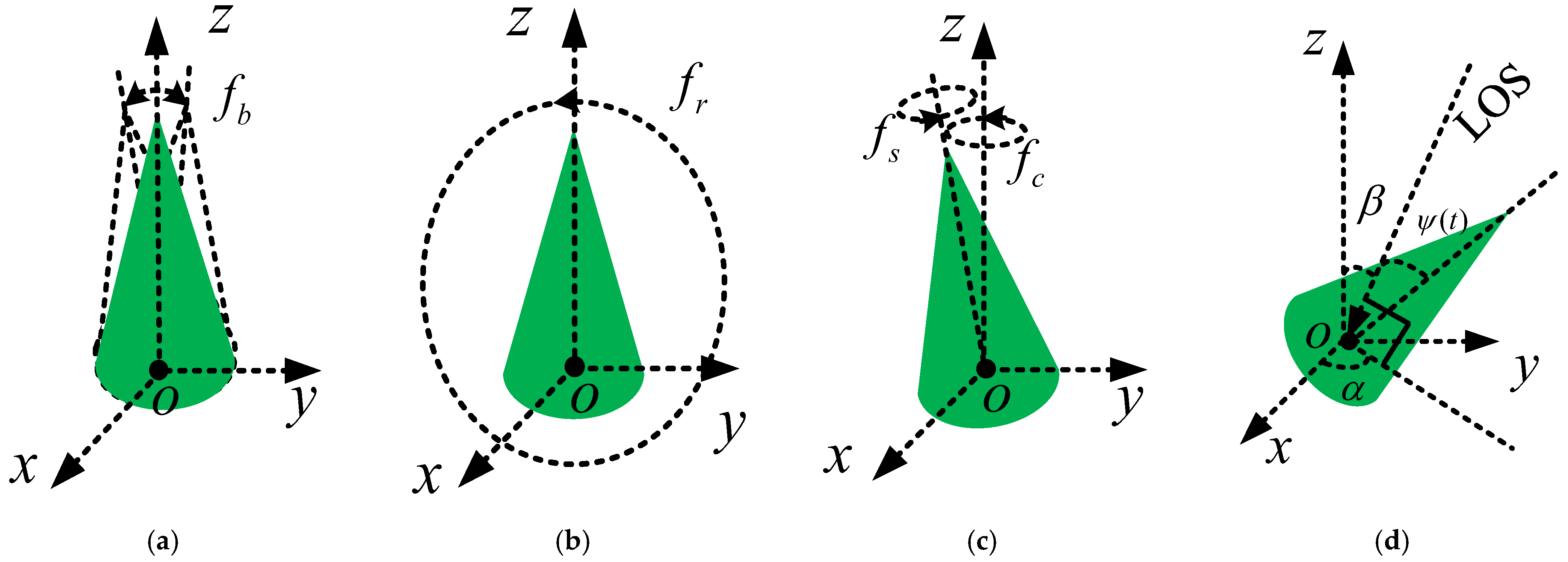
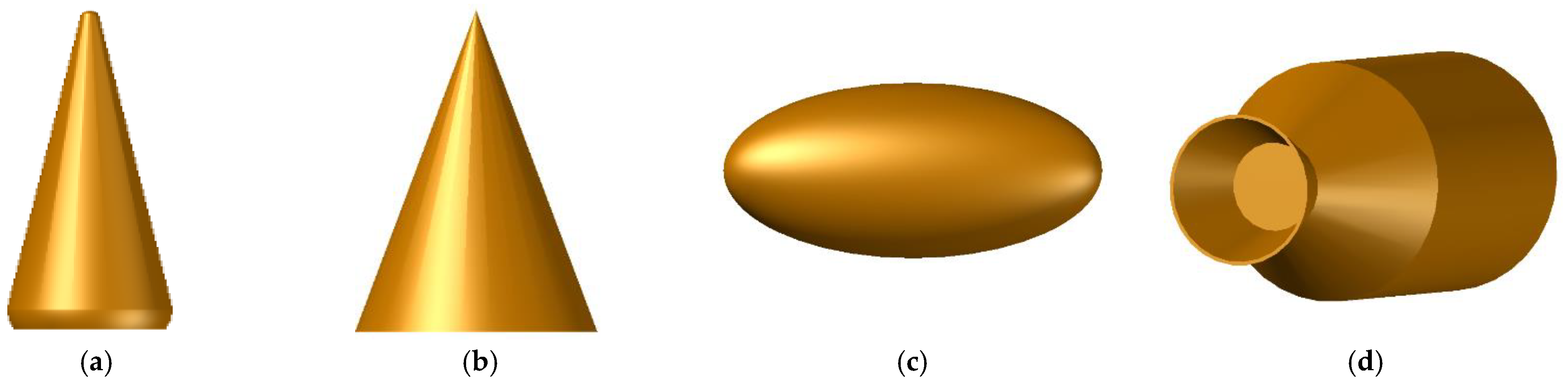
2. The Micro-Motion Model of BTs
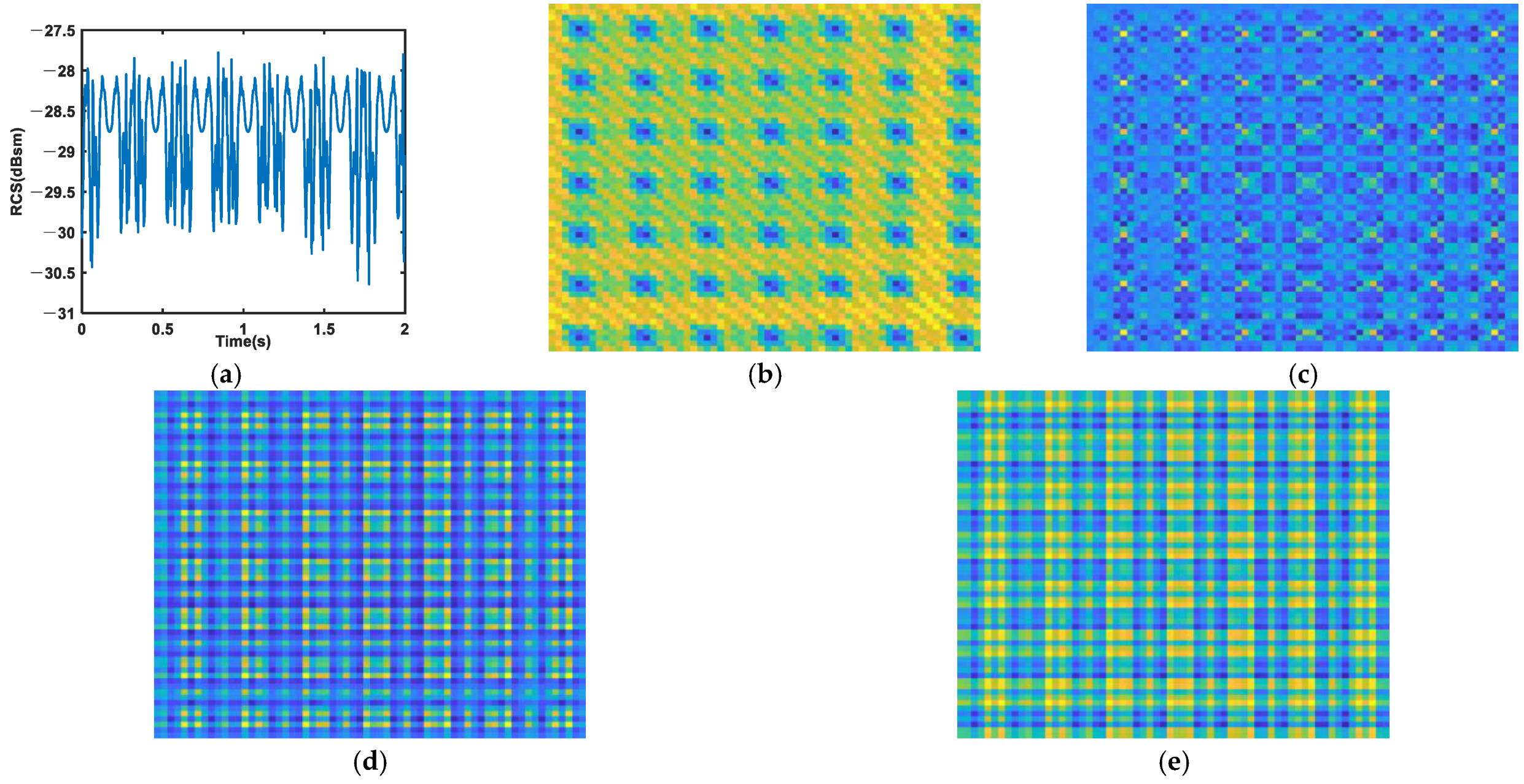
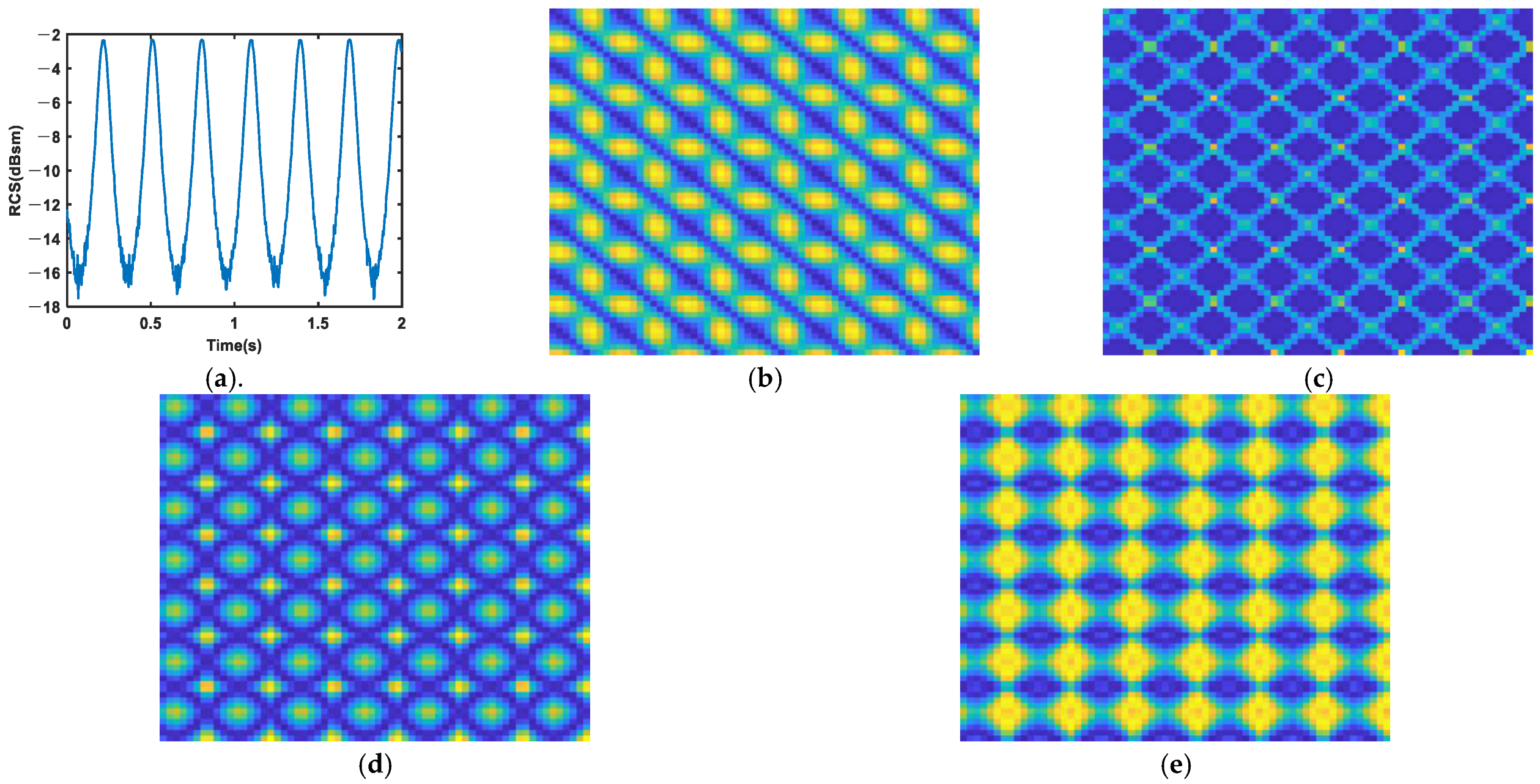
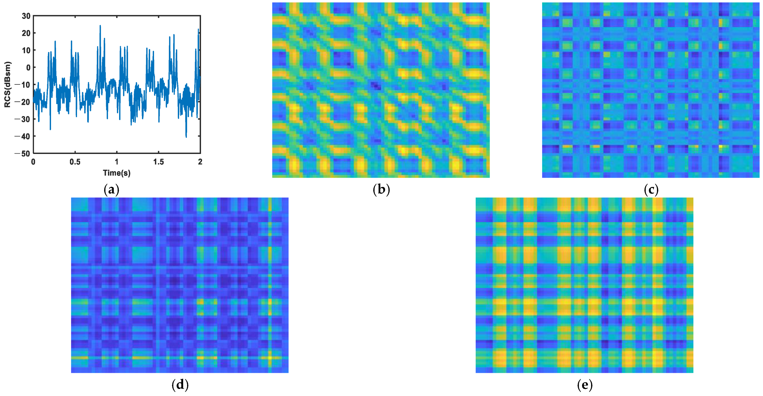
3. Methods for RCS Sequences Encoding
3.1. MTF
3.2. GAF
3.3. RP
4. Proposed Network
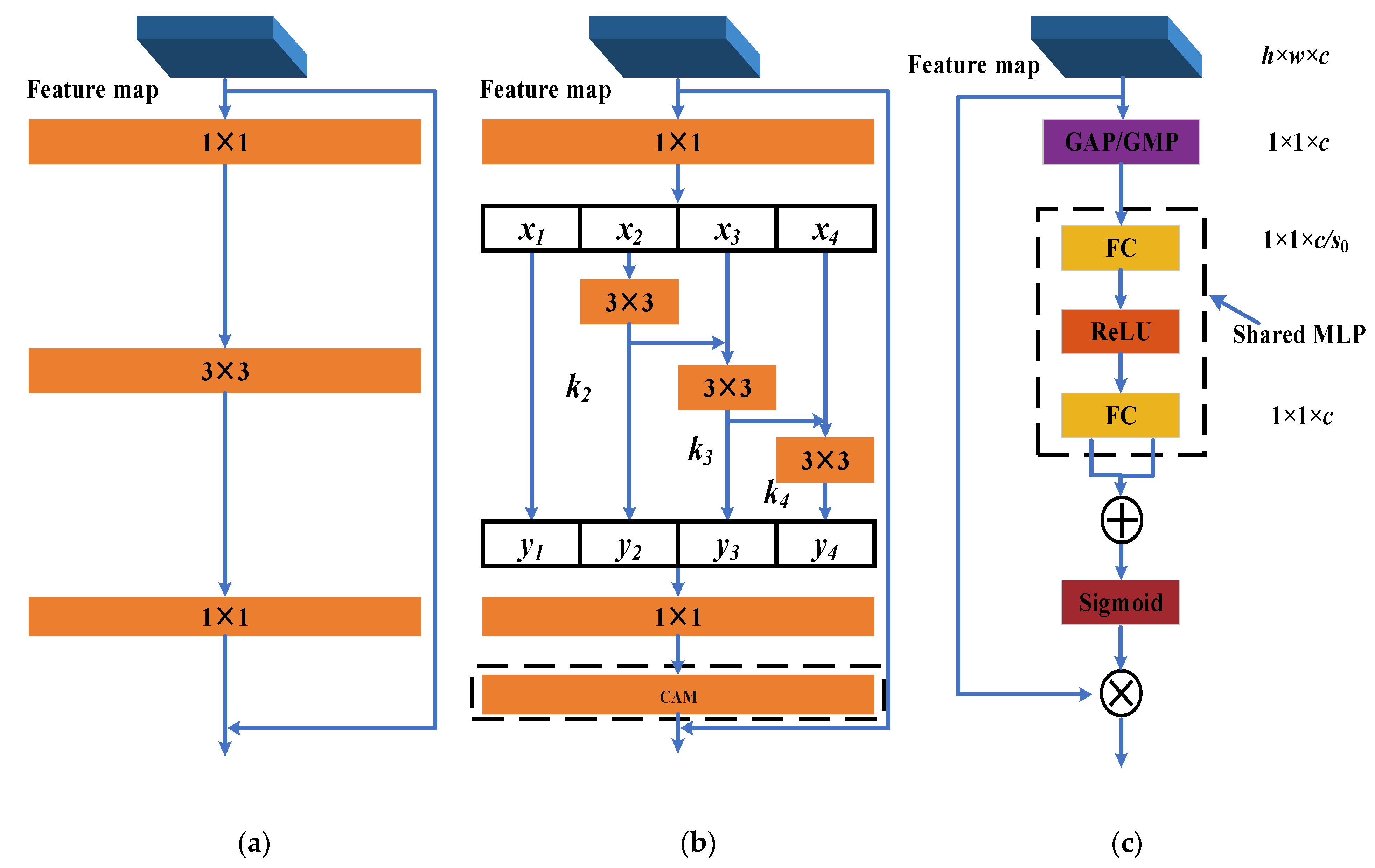
4.1. Res2Net
4.2. Channel Attention
4.3. The Activation Function (AF) and the Loss Function
5. Experiments
6. Conclusions
Author Contributions
Funding
Data Availability Statement
Conflicts of Interest
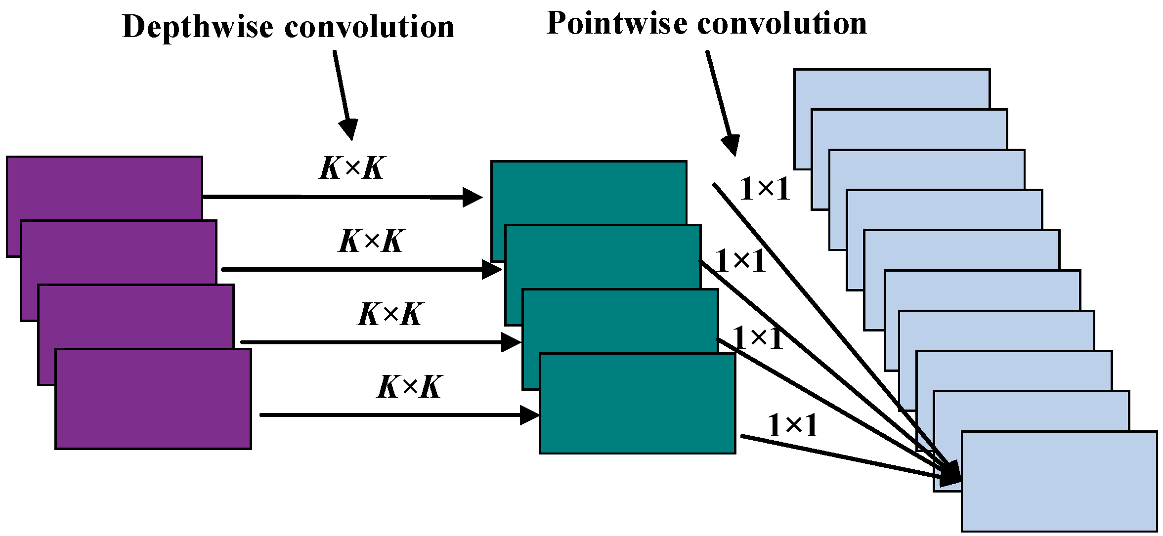
Appendix A. Depthwise Separable Convolution (DS-Conv)

References
- Tahmoush, D.; Ling, H.; Stankovic, L.; Thayaparan, T.; Narayanan, R. Current Research in Micro-Doppler: Editorial for the Special Issue on Micro-Doppler. IET Radar Sonar Nav. 2015, 9, 1137–1139. [Google Scholar] [CrossRef]
- Choi, I.; Jung, J.; Kim, K.; Park, S. Effective Discrimination between Warhead and Decoy in Mid-Course Phase of Ballistic Missile. J. Korean Inst. Electromagn. Eng. Sci. 2020, 31, 468–477. [Google Scholar] [CrossRef]
- Zhang, W.P.; Li, K.L.; Jiang, W.D. Parameter Estimation of Radar Targets with Macro-Motion and Micro-Motion Based on Circular Correlation Coefficients. IEEE Signal Proc. Lett. 2015, 22, 633–637. [Google Scholar] [CrossRef]
- Chen, X.L.; Zhang, H.; Song, J.; Guan, J.; Li, J.F.; He, Z.W. Micro-Motion Classification of Flying Bird and Rotor Drones via Data Augmentation and Modified Multi-Scale CNN. Remote Sens. 2022, 14, 1107. [Google Scholar] [CrossRef]
- Kim, B.K.; Kang, H.S.; Park, S.O. Drone Classification Using Convolutional Neural Networks With Merged Doppler Images. IEEE Geosci. Remote S 2017, 14, 38–42. [Google Scholar] [CrossRef]
- Zhu, N.; Xu, S.; Li, C.; Hu, J.; Fan, X.; Wu, W.; Chen, Z. An Improved Phase-Derived Range Method Based on High-Order Multi-Frame Track-Before-Detect for Warhead Detection. Remote Sens. 2022, 14, 29. [Google Scholar] [CrossRef]
- Zhu, N.; Hu, J.; Xu, S.; Wu, W.; Zhang, Y.; Chen, Z. Micro-Motion Parameter Extraction for Ballistic Missile with Wideband Radar Using Improved Ensemble EMD Method. Remote Sens. 2021, 13, 3545. [Google Scholar] [CrossRef]
- He, F.Y.; Xiao, Z.Y. Micro-motion modelling and analysis of extended ballistic targets based on inertial parameters. Electron. Lett. 2013, 49, 129–130. [Google Scholar] [CrossRef]
- Gao, H.; Xie, L.; Wen, S.; Kuang, Y. Micro-Doppler Signature Extraction from Ballistic Target with Micro-Motions. IEEE Trans. Aerosp. Electron. Syst. 2010, 46, 1969–1982. [Google Scholar] [CrossRef]
- Han, L.; Feng, C. Micro-Doppler-Based Space Target Recognition with a One-Dimensional Parallel Network. Int. J. Antennas Propag. 2020, 2020, 8013802. [Google Scholar] [CrossRef]
- Hanif, A.; Muaz, M.; Hasan, A.; Adeel, M. Micro-Doppler Based Target Recognition With Radars: A Review. IEEE Sens. J. 2022, 22, 2948–2961. [Google Scholar] [CrossRef]
- Choi, I.O.; Park, S.H.; Kim, M.; Kang, K.B.; Kim, K.T. Efficient Discrimination of Ballistic Targets With Micromotions. IEEE Trans. Aerosp. Electron. Syst. 2020, 56, 1243–1261. [Google Scholar] [CrossRef]
- Choi, I.O.; Jung, J.H.; Kim, K.T.; Riggs, L.; Kim, S.H.; Park, S.H. Efficient 3DFV for improved discrimination of ballistic warhead. Electron Lett. 2018, 54, 1452–1453. [Google Scholar] [CrossRef]
- Jung, K.; Lee, J.I.; Kim, N.; Oh, S.; Seo, D.W. Classification of Space Objects by Using Deep Learning with Micro-Doppler Signature Images. Sensors 2021, 21, 4365. [Google Scholar] [CrossRef]
- Zhang, Y.P.; Zhang, Q.; Kang, L.; Luo, Y.; Zhang, L. End-to-End Recognition of Similar Space Cone–Cylinder Targets Based on Complex-Valued Coordinate Attention Networks. IEEE Trans. Geosci. Remote Sens. 2022, 60, 1–14. [Google Scholar] [CrossRef]
- Daiying, Z.; Jianhui, Y. Ballistic target recognition based on micro-motion characteristics using sequential HRRPs. In Proceedings of the 2013 IEEE 4th International Conference on Electronics Information and Emergency Communication, Beijing, China, 15–17 November 2013; pp. 165–168. [Google Scholar]
- Persico, A.R.; Ilioudis, C.V.; Clemente, C.; Soraghan, J.J. Novel Classification Algorithm for Ballistic Target Based on HRRP Frame. IEEE Trans. Aerosp. Electron. Syst. 2019, 55, 3168–3189. [Google Scholar] [CrossRef] [Green Version]
- Wang, Y.Z.; Feng, C.Q.; Hu, X.W.; Zhang, Y.S. Classification of Space Micromotion Targets With Similar Shapes at Low SNR. IEEE Geosci. Remote Sens. Lett. 2021, 19, 1–5. [Google Scholar] [CrossRef]
- Cai, T.; Sheng, Y.; He, Z.; Sun, W. Classification and recognition of ballistic microcephalus based on deep neural network. In Proceedings of the 2019 International Applied Computational Electromagnetics Society Symposium, Nanjing, China, 8–11 August 2019; pp. 1–2. [Google Scholar]
- Ye, L.; Hu, S.B.; Yan, T.T.; Meng, X.; Zhu, M.Q.; Xu, R.Z. Radar target shape recognition using a gated recurrent unit based on RCS time series’ statistical features by sliding window segmentation. IET Radar Sonar Navig. 2021, 15, 1715–1726. [Google Scholar] [CrossRef]
- Chen, J.; Xu, S.Y.; Chen, Z.P. Convolutional neural network for classifying space target of the same shape by using RCS time series. IET Radar Sonar Navig. 2018, 12, 1268–1275. [Google Scholar] [CrossRef]
- Noori, F.M.; Riegler, M.; Uddin, M.Z.; Torresen, J. Human Activity Recognition from Multiple Sensors Data Using Multi-fusion Representations and CNNs. ACM Trans. Multimedia Comput. Commun. Appl. 2020, 16, 1–19. [Google Scholar] [CrossRef]
- Tian, X.; Bai, X.; Xue, R.; Qin, R.; Zhou, F. Fusion Recognition of Space Targets With Micromotion. IEEE Trans. Aerosp. Electron. Syst. 2022, 58, 3116–3125. [Google Scholar] [CrossRef]
- Zhao, X.; Sun, H.; Lin, B.; Zhao, H.; Niu, Y.; Zhong, X.; Wang, Y.; Zhao, Y.; Meng, F.; Ding, J.; et al. Markov Transition Fields and Deep Learning-Based Event-Classification and Vibration-Frequency Measurement for φ-OTDR. IEEE Sens. J. 2022, 22, 3348–3357. [Google Scholar] [CrossRef]
- Esmael, A.A.; da Silva, H.H.; Ji, T.; Torres, R.D. Non-Technical Loss Detection in Power Grid Using Information Retrieval Approaches: A Comparative Study. IEEE Access 2021, 9, 40635–40648. [Google Scholar] [CrossRef]
- Paulo, J.R.; Pires, G.; Nunes, U.J. Cross-Subject Zero Calibration Driver’s Drowsiness Detection: Exploring Spatiotemporal Image Encoding of EEG Signals for Convolutional Neural Network Classification. IEEE Trans. Neural Syst. Rehabil. Eng. 2021, 29, 905–915. [Google Scholar] [CrossRef] [PubMed]
- Wang, Z.; Oates, T. Spatially Encoding Temporal Correlations to Classify Temporal Data Using Convolutional Neural Networks. arXiv 2015, arXiv:1509.07481. [Google Scholar]
- Zhang, Y.; Hou, Y.; OuYang, K.; Zhou, S. Multi-scale signed recurrence plot based time series classification using inception architectural networks. Pattern Recognit. 2022, 123, 108385. [Google Scholar] [CrossRef]
- Dias, D.; Pinto, A.; Dias, U.; Lamparelli, R.; Le Maire, G.; Torres, R.D. A Multirepresentational Fusion of Time Series for Pixelwise Classification. IEEE J. Sel. Top. Appl. Earth Obs. Remote Sens. 2020, 13, 4399–4409. [Google Scholar] [CrossRef]
- Faustine, A.; Pereira, L.; Klemenjak, C. Adaptive Weighted Recurrence Graphs for Appliance Recognition in Non-Intrusive Load Monitoring. IEEE Trans. Smart Grid 2021, 12, 398–406. [Google Scholar] [CrossRef]
- Deng, Q.Q.; Lu, H.Z.; Hu, M.F.; Zhao, B.D. Exo-atmospheric infrared objects classification using recurrence-plots-based convolutional neural networks. Appl. Optics 2019, 58, 164–171. [Google Scholar] [CrossRef]
- Pham, T.D. Pattern analysis of computer keystroke time series in healthy control and early-stage Parkinson’s disease subjects using fuzzy recurrence and scalable recurrence network features. J. Neurosci Meth. 2018, 307, 194–202. [Google Scholar] [CrossRef]
- Pham, T.D.; Wardell, K.; Eklund, A.; Salerud, G. Classification of Short Time Series in Early Parkinson’s Disease With Deep Learning of Fuzzy Recurrence Plots. IEEE-CAA J. Autom. Sin. 2019, 6, 1306–1317. [Google Scholar] [CrossRef]
- Zhang, Z.; Luo, H.; Wang, C.; Gan, C.; Xiang, Y. Automatic Modulation Classification Using CNN-LSTM Based Dual-Stream Structure. IEEE Trans. Veh. Technol. 2020, 69, 13521–13531. [Google Scholar] [CrossRef]
- Xie, X.J.; Peng, S.L.; Yang, X. Deep Learning-Based Signal-To-Noise Ratio Estimation Using Constellation Diagrams. Mob. Inf Syst. 2020, 2020, 1–9. [Google Scholar] [CrossRef]
- Gao, S.H.; Cheng, M.M.; Zhao, K.; Zhang, X.Y.; Yang, M.H.; Torr, P. Res2Net: A New Multi-Scale Backbone Architecture. IEEE Trans. Pattern Anal. Mach. Intell. 2021, 43, 652–662. [Google Scholar] [CrossRef] [Green Version]
- Que, Y.; Li, S.L.; Lee, H.J. Attentive Composite Residual Network for Robust Rain Removal from Single Images. IEEE Trans. Multimedia 2021, 23, 3059–3072. [Google Scholar] [CrossRef]
- Woo, S.H.; Park, J.; Lee, J.Y.; Kweon, I.S. CBAM: Convolutional Block Attention Module. In Proceedings of the 15th European Conference on Computer Vision (ECCV), Munich, Germany, 8–14 September 2018; pp. 3–19. [Google Scholar]
- Dubey, S.R.; Singh, S.K.; Chaudhuri, B.B. Activation functions in deep learning: A comprehensive survey and benchmark. Neurocomputing 2022, 503, 92–108. [Google Scholar] [CrossRef]
- Tang, W.; Yu, L.; Wei, Y.; Tong, P. Radar Target Recognition of Ballistic Missile in Complex Scene. In Proceedings of the 2019 IEEE International Conference on Signal, Information and Data Processing (ICSIDP), Chongqing, China, 11–13 December 2019; pp. 1–6. [Google Scholar]
- Kim, I.H.; Choi, I.S.; Chae, D.Y. A Study on the Performance Enhancement of Radar Target Classification Using the Two-Level Feature Vector Fusion Method. J. Electromagn. Eng. Sci. 2018, 18, 206–211. [Google Scholar] [CrossRef] [Green Version]
- Che, J.; Wang, L.; Bai, X.; Liu, C.; Zhou, F. Spatial-Temporal Hybrid Feature Extraction Network for Few-shot Automatic Modulation Classification. IEEE Trans. Veh. Technol. 2022, 1–6. [Google Scholar] [CrossRef]
- Cheng, M.; Wang, H.L.; Long, Y. Meta-Learning-Based Incremental Few-Shot Object Detection. IEEE Trans. Circuits Syst. Video Technol. 2022, 32, 2158–2169. [Google Scholar] [CrossRef]
- Quan, J.N.; Ge, B.Z.; Chen, L. Cross attention redistribution with contrastive learning for few shot object detection. Displays 2022, 72, 102162. [Google Scholar] [CrossRef]
- Chollet, F. Xception: Deep Learning with Depthwise Separable Convolutions. In Proceedings of the 2017 IEEE Conference on Computer Vision and Pattern Recognition (CVPR), Honolulu, HI, USA, 21–26 July 2017; pp. 1800–1807. [Google Scholar]
- Muhammad, W.; Aramvith, S.; Onoye, T. Multi-scale Xception based depthwise separable convolution for single image super-resolution. PLoS ONE 2021, 16, 20. [Google Scholar] [CrossRef] [PubMed]


| Order | Shortcut | Cycle | Operation | Output Size |
|---|---|---|---|---|
| 1 | — | — | Input | 64 × 64 × 1 |
| 2 | — | — | Conv 32.3 × 3, stride = 1 | 62 × 62 × 32 |
| 3 | — | — | Conv 128.3 × 3, stride = 1 | 62 × 62 × 128 |
| 4 | — | — | Maxpooling, 3 × 3, stride = 2 | 30 × 30 × 128 |
| 5 | — | — | Res2net 128-256-128 | 30 × 30 × 128 |
| 6 | Conv 1 × 1, stride = 2 | — | DS-Conv 768.3 × 3, stride = 1 DS-Conv 768.3 × 3, stride = 1 Maxpooling, 3 × 3, stride = 2 | 15 × 15 × 768 |
| 7 | — | 2 | Res2net | 15 × 15 × 768 |
| 8 | — | CAM-Res2net | 15 × 15 × 768 | |
| 9 | Conv 1 × 1, stride = 2 | — | DS-Conv 1024.3 × 3, stride = 1 DS-Conv 1024.3 × 3, stride = 1 Maxpooling, 3 × 3, stride = 2 | 8 × 8 × 1024 |
| 10 | — | — | CAM-Res2net | 8 × 8 × 1024 |
| 11 | — | — | DS-Conv 256.3 × 3, stride = 1 | 8 × 8 × 256 |
| 12 | — | — | Global Avgpooling | 1 × 1 × 256 |
| 13 | — | — | Dropout 0.2 | 1 × 1 × 256 |
| 14 | — | — | Fc 4 | 1 × 1 × 4 |
| 15 | — | — | Output | Predicted label |
| Warhead | Heavy Decoy | Light Decoy | Booster | |
|---|---|---|---|---|
| Precession | Swing | Rolling | Rolling | |
| − | − | − | ||
| − | − | − | ||
| − | − | |||
| − | − | − | ||
| − | − | − |
| Warhead | Weight Decoy | Light Decoy | Booster | ||
|---|---|---|---|---|---|
| Recall | Accuracy | ||||
| 4 | 0.8854 | 0.7474 | 0.8964 | 0.9125 | 0.8604 |
| 8 | 0.9219 | 0.7604 | 0.9115 | 0.9427 | 0.8841 |
| 16 | 0.9083 | 0.7724 | 0.8828 | 0.9323 | 0.8740 |
| 32 | 0.8906 | 0.7380 | 0.8573 | 0.8875 | 0.8434 |
| 64 | 0.7953 | 0.6510 | 0.8224 | 0.7917 | 0.7651 |
| Warhead | Weight Decoy | Light Decoy | Booster | ||
|---|---|---|---|---|---|
| Recall | Accuracy | ||||
| GASF | 0.9323 | 0.7917 | 0.9115 | 0.9740 | 0.9023 |
| GADF | 0.9167 | 0.7708 | 0.9479 | 0.9167 | 0.8880 |
| Warhead | Weight Decoy | Light Decoy | Booster | ||
|---|---|---|---|---|---|
| Recall | Accuracy | ||||
| (1, 1) | 0.9573 | 0.8891 | 0.9599 | 0.9938 | 0.9500 |
| (1, 3) | 0.9526 | 0.8844 | 0.9620 | 0.9923 | 0.9478 |
| (1, 5) | 0.9635 | 0.8734 | 0.9609 | 0.9932 | 0.9478 |
| (4, 3) | 0.9547 | 0.8734 | 0.9740 | 0.9953 | 0.9493 |
| (7, 3) | 0.9620 | 0.8990 | 0.9484 | 0.9953 | 0.9512 |
| (4, 5) | 0.9635 | 0.9010 | 0.9531 | 0.9792 | 0.9492 |
| (4, 7) | 0.9672 | 0.8776 | 0.9599 | 0.9958 | 0.9501 |
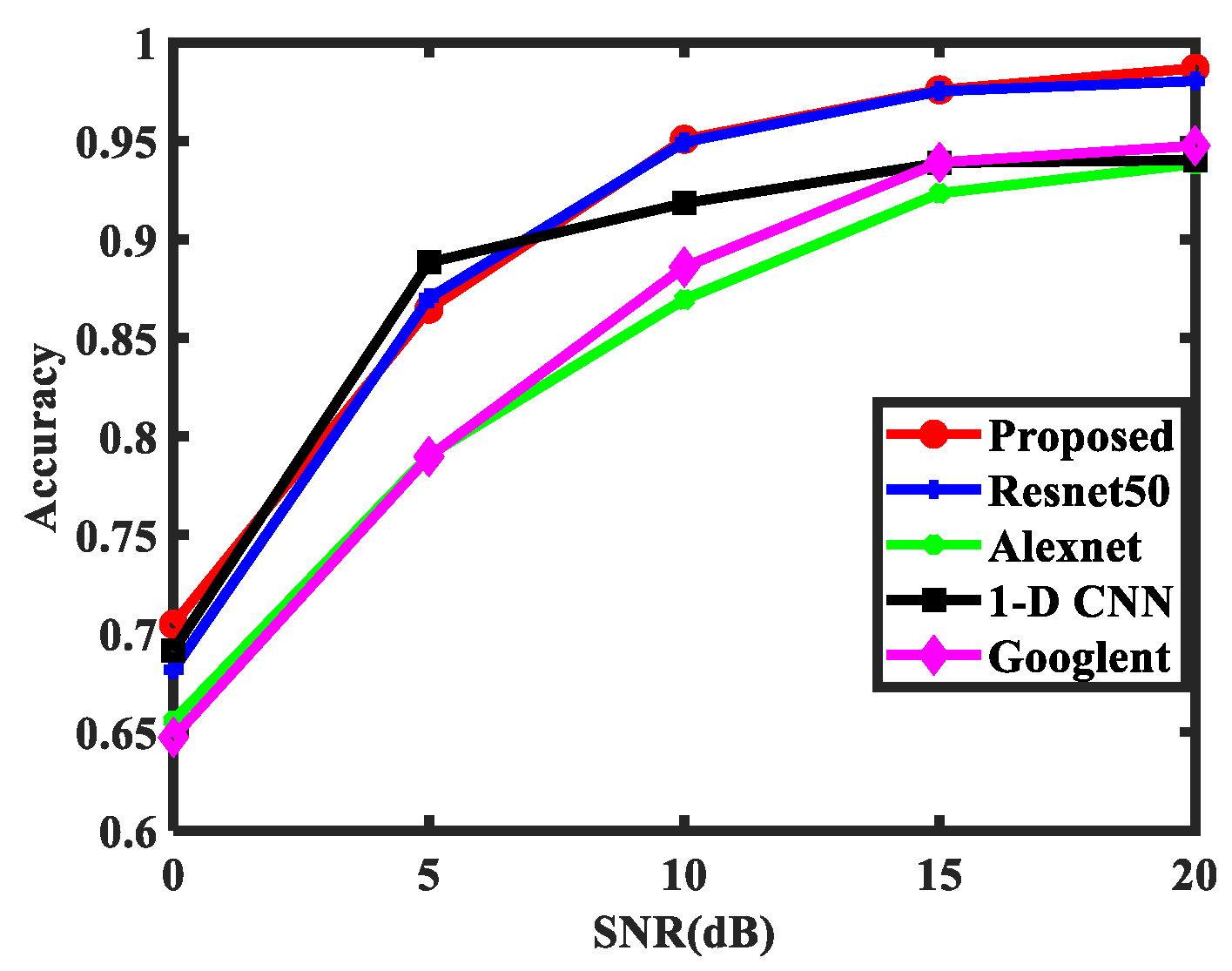
| 20 dB | 15 dB | 10 dB | 5 dB | 0 dB | |
|---|---|---|---|---|---|
| Resnet50 | 0.9802 | 0.9752 | 0.9493 | 0.8697 | 0.6822 |
| Googlenet | 0.9470 | 0.9387 | 0.8847 | 0.7838 | 0.6306 |
| Alexnet | 0.9373 | 0.9226 | 0.8672 | 0.7845 | 0.6387 |
| 1D CNN | 0.9390 | 0.9370 | 0.9153 | 0.8815 | 0.6938 |
| Proposed | 0.9868 | 0.9758 | 0.9507 | 0.8639 | 0.7013 |
| Resnet50 | Googlenet | Alexnet | 1D CNN | Proposed | |
|---|---|---|---|---|---|
| Time(us) | 17.38 | 12.66 | 5.3701 | 4.3546 | 33.79 |
Publisher’s Note: MDPI stays neutral with regard to jurisdictional claims in published maps and institutional affiliations. |
© 2022 by the authors. Licensee MDPI, Basel, Switzerland. This article is an open access article distributed under the terms and conditions of the Creative Commons Attribution (CC BY) license (https://creativecommons.org/licenses/by/4.0/).
Share and Cite
Xu, X.; Feng, C.; Han, L. Classification of Radar Targets with Micro-Motion Based on RCS Sequences Encoding and Convolutional Neural Network. Remote Sens. 2022, 14, 5863. https://doi.org/10.3390/rs14225863
Xu X, Feng C, Han L. Classification of Radar Targets with Micro-Motion Based on RCS Sequences Encoding and Convolutional Neural Network. Remote Sensing. 2022; 14(22):5863. https://doi.org/10.3390/rs14225863
Chicago/Turabian StyleXu, Xuguang, Cunqian Feng, and Lixun Han. 2022. "Classification of Radar Targets with Micro-Motion Based on RCS Sequences Encoding and Convolutional Neural Network" Remote Sensing 14, no. 22: 5863. https://doi.org/10.3390/rs14225863