1. Introduction
The electromagnetic environment of radar is becoming increasingly complex with the advancement of modern electronic jamming technology, and new types of jamming are occurring more regularly [
1,
2,
3,
4,
5]. Many intelligent technologies are applied in the field of radar detection and anti-jamming. Jamming recognition technologies are important for modern radars. It is an important prerequisite to ensure that we can successfully counter enemy jamming measures in electronic warfare. Only by correctly identifying the jamming signal emitted by the jammer can the corresponding measures for specific types of jamming be implemented. Hence, the radar jamming recognition module plays a primary role in the intelligent radar system. The high performance of the radar jamming recognition module is the prerequisite for the intelligent anti-jamming system to obtain an excellent effect.
The applications of radar in military and civil areas have rapidly progressed due to the extensive development of machine learning and deep learning technologies. Recently, some researchers have combined technologies of machine learning and radars to implement identity authentication. Among these researches, radar has shown great promise in healthcare applications as it requires neither contact nor line-of-sight and does not give rise to privacy concerns associated with video imaging [
6,
7,
8]. Technologies of deep learning have also been used in the field of smart grids. A smart detection method based on secure federated deep learning is proposed to prevent false data injection attacks (FDIA) [
9]. A deep learning-based short-term voltage stability (STVSA) model has been proposed which achieves higher accuracy in the case of small samples compared with the previous methods [
10]. The two categories of radar jamming recognition methods are feature extraction-based [
11] and deep learning-based methods [
12]. A convolutional neural network (CNN)-based radar jamming recognition method was proposed in 2019, first using the time-frequency images of the various jamming signals as the CNN inputs [
13]. A weighted integrated CNN radar jamming recognition algorithm based on transfer learning was proposed in 2021 for the low recognition accuracy of deep learning jamming recognition methods in the case of small samples [
14]. A jamming recognition method based on Residual Neural Network (ResNet) was proposed in 2021, using the bispectrum diagonal slice extracted from the jamming signals as the input of ResNet to realize the recognition of active deception jamming [
15].
However, some problems in the current radar jamming recognition methods remain to be solved: Existing radar jamming recognition methods assume that the types of jamming signals in the testing environment are the same as those in the training jamming library. With this assumption, jamming recognition is referred to as close set recognition. When radars detect an unknown type of jamming in the actual open set jamming scenario, the existing radar jamming recognition models will incorrectly identify it as a known type of jamming in the training jamming library. Nevertheless, jammers and radars are encountered in the actual situation. Moreover, new types of jamming signals are constantly developed. Consequently, collecting all types of jamming data would be difficult for the training jamming library of our jamming recognition model. Hence, the actual radar jamming environment is the open set environment. In particular, the type of jamming that does not exist in the training jamming library is likely to occur in the testing environment. The recognition in the open set environment is called open set recognition (OSR), and it has already been utilized in the fields of image recognition [
16].
Most of the original OSR models are implemented by using support vector machines (SVM) to constrain some parts of the open space [
16,
17,
18,
19]. Some of them can only distinguish whether the test samples belong to known or unknown sample, but cannot classify which class the known samples belong to [
20]. With the gradual deepening of research in this field, recognition models that can distinguish unknown types and correctly identify known types begin to appear [
21], and OSR is successfully implemented using deep learning networks [
21,
22,
23]. Scheierer [
16] introduced the concept of OSR and proposed the 1-vs-set model from the perspective of constraining open space, which is the first OSR model. The 1-vs-set model distinguishes known and unknown targets by using two parallel hyperplanes that do not effectively utilize the open space. Quasi-linear discriminants are suggested to overcome this problem, which outperform the 1-vs-set model proposed by Scheierer. These discriminants can be trained from either binary or positive-only samples by using constrained quadratic programs related to SVMs [
24]. Bendale and Boult [
13] proposed a deep neural network model for OSR by introducing the OpenMax layer to estimate the probability of an unknown class, which pioneered the use of deep neural networks in OSR. OpenMax has been used in text classification to solve the open set text classification problem, and has achieved good performance [
21].
In the face of increasingly complex electromagnetic environments, radar jamming recognition needs the ability to operate normally in open set scenarios. This requires that the radar not only classifies the known jamming accurately, but also distinguishes the unknown jamming correctly so that specific anti-jamming measures can be implemented promptly. We urgently need to find an intelligent recognition model that enables radar to automatically process unknown jamming signals. In view of the great success of the deep learning method in the classification and recognition of radar jamming signals, we hope to use the deep learning model to achieve the OSR for radar jamming signals. For these reasons, we propose two OSR models to address the open set problem in the radar anti-jamming environment so that radars can recognize the known jamming and distinguish the unknown: a model based on the confidence score and a model based on OpenMax. The OSR model based on the confidence score quantifies the difference between known and unknown classes based on the probability distribution of their output and sets a threshold to realize the discrimination of known and unknown types. The probability distribution of known jamming is concentrated on one class. By contrast, the probability distribution of unknown jamming is more uniform. The OSR model based on OpenMax replaces the SoftMax layer with the OpenMax layer by altering the full connection layer of the second-last layer of the original classifier (the previous layer of the SoftMax layer). The modified OpenMax layer outputs the probability that the jamming samples belong to each known class and the probability that they belong to the unknown class. OSR is achieved by using the category to which the highest probability of the output probability distribution belongs as the classification result. The main contributions of this work are as follows: First, we introduce the concept of OSR in the radar jamming recognition. Second, we propose the confidence score-based model to distinguish unknown types of jamming signals. Third, we combine the OSR models with the deep networks in the intelligent jamming recognition module.
In this paper,
Section 2 introduces the common jamming signals and their time-frequency images.
Section 3 introduces the open set jamming recognition models proposed in this work.
Section 4 introduces several experiments to verify the performance of the OSR model.
Section 5 summarizes the main work of this paper and provides a conclusion.
2. Jamming Signal Analysis
Radar jamming can be divided into intentional and unintentional jamming according to the purpose. Meanwhile, intentional jamming can be divided into active and passive jamming. Radar active jamming can be divided into three categories: suppression, deceptive, and composite jamming [
25].
This section introduces the jamming signal model and time-frequency domain images of active radar jamming. The types of jamming signals vary in the actual scenarios. Among the three types of jamming signals, suppression jamming interferes with radar in specific frequency bands through high-energy jamming signals, rendering radar ineffective in these bands. Deceptive jamming interferes with radar by sending many false targets to it, making it impossible for the radar to detect the real target. Composite jamming combines the advantages of suppression jamming and deceptive jamming. This mechanism prevents the radar from normally operating in a specific frequency band and detects a significant number of false targets.
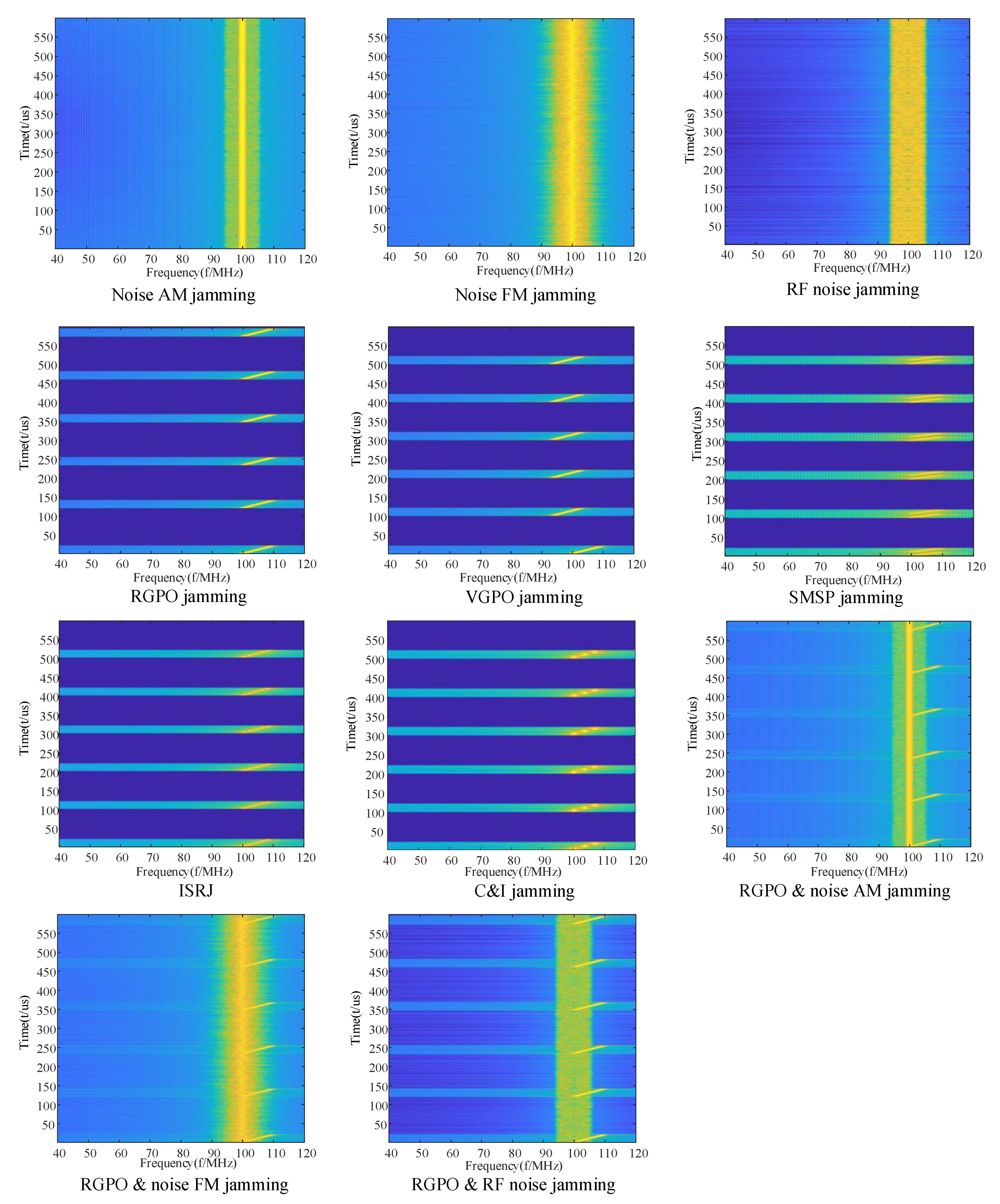
Eleven types of common jamming signals are simulated to verify the validity of jamming recognition models proposed in this work. As shown in
Figure 1, the three types of suppression jamming include noise amplitude modulation (AM) jamming, noise frequency modulation (FM) jamming, and radio frequency (RF) noise jamming. Meanwhile, deceptive jamming includes range gate pull-off (RGPO) jamming, velocity gate pull-off (VGPO) jamming, smeared spectrum (SMSP) jamming, interrupted sampling repeater jamming (ISRJ), and chopping and interleaving (C&I) jamming. Among these types of deceptive jamming, RGPO and VGPO jamming can produce a single false target with the incorrect distance or velocity. SMSP jamming, ISRJ, and C&I jamming can produce multiple false targets by modulating and retransmitting the signal saved in the digital radio frequency memory system. Composite jamming includes RGPO and noise AM jamming, RGPO and noise FM jamming, and RGPO and RF noise jamming, which are additive jamming. These 11 types of jamming signals are simulated according to the generation mechanism [
1,
2,
3,
4,
5], and the simulation results are shown in
Section 4.
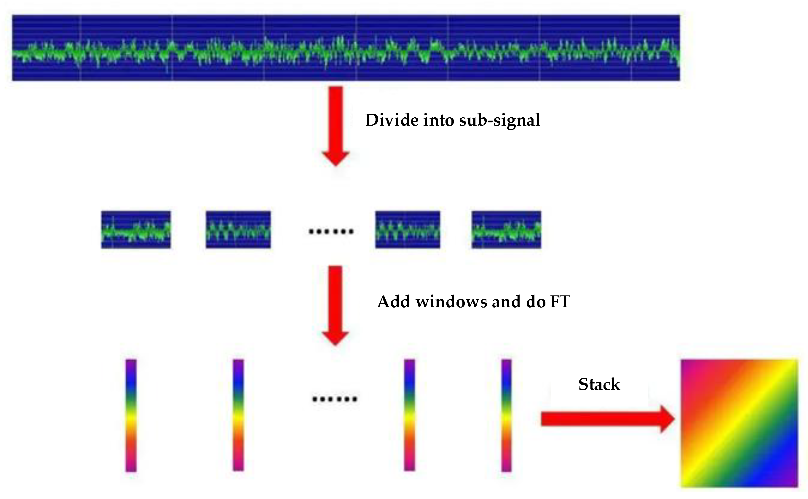
After the radar active jamming signal is obtained, we convert it into a time–frequency image by short-time Fourier transform (STFT) and take the time–frequency image of active radar jamming as a dataset to provide a data basis for the subsequent jamming classification [
26]. The operation process of STFT is shown in
Figure 2.
STFT operates as follows:
Divide the signal into several sub-signals.
Add windows and perform Fourier transform (FT) for each sub-signal.
Combine the Fourier transform results of each sub-signal.
Thereafter, the time–frequency image of jamming signal can be obtained. The mathematical expression of STFT is shown as follows:
where
is the jamming signal to be analyzed,
is the window function, and
is the Fourier transform of sub-signal
.
We convert 1D time–domain signals into 2D time–frequency images through STFT to ensure that the data can provide information in time–domain and frequency–domain dimensions and can be directly used as the CNN inputs.
3. Two Models of Open Set Recognition
Most current jamming recognition techniques assume that the radar is in a closed environment. In particular, the type of jamming radar encountered during training is the same as that encountered during testing, and there is no unknown type of jamming in the testing set that is not present in the training set.
By contrast, with the constant appearance of new jamming types, there is no guarantee that the jamming detected in the actual situation would be known in advance during training, and the previously assumed close set scenarios are increasingly unsuitable for radar jamming recognition. In this work, the concept of open set is introduced in radar jamming detection. Specifically, an unknown jamming is detected that does not arise during training.
Figure 3 shows the open set environment. The recognition ability of radar in a complex electromagnetic environment is improved by studying the recognition method of jamming signals in open set scenes.
The following describes the OSR definition [
27]:
Definition 1 (OSR). The training and test sets consisting of sample-label pairs are represented as follows:whereandare the training and testing sets, respectively;are the training and testing samples;andare the labels of;are the numbers of training and testing samples;are the sets of training and testing samples;andare the label sets of the training and testing samples; andis the label set inbut not in.
We define that . Accordingly, more labels are present in the testing set that do not appear in the training set. OSR uses training set to learn a recognition model that can correctly classify the known categories and accurately distinguish the unknown categories .
The following part of this section will introduce the pre-training networks used for the OSR models.
3.1. Pre-Training Networks
Before the OSR, a pre-training neural network should be chosen as the radar jamming classifier. Herein, we select the CNN model based on transfer learning as a classifier for jamming recognition to ensure that the model has better generalization performance and is not easy to overfit. The original domain dataset for transfer learning is the ImageNet [
28], which includes more than 14 million labeled images and covers more than 2000 categories. The target area is the time–frequency image of the jamming signal. The ImageNet dataset fully meets the requirements of the original domain dataset for transfer learning. Accordingly, the pre-training model used for transfer learning can obtain sufficient prior knowledge from ImageNet. The pre-training model based on transfer learning causes the jamming recognition model to converge faster with less overfit during training [
29].
The common modes for transfer learning include feature, instance, and model transfers. Among these modes, model transfer is one of the most commonly used transfer learning methods in deep learning [
30]. Model transfer refers to training a deep learning model (also known as a pre-training model) in the original domain, then transferring the parameters of the pre-training model to the recognition model in the target domain, and finally training the recognition model on the small sample dataset to obtain the small sample recognition model. The training process of model-based transfer learning is shown in
Figure 4.
The network structure is presented in
Figure 5. The model’s input data is the time–frequency image of the active jamming signal. The structure of the model consists of two parts: the classification model based on ImageNet and the shallow CNN classification model. First, we construct a network with the same parameters as the network trained by the ImageNet dataset and use it as the feature extraction network for jamming time–frequency images. Then, we train a shallow network to obtain the recognition results through the jamming feature output by the deep network.
3.2. OSR Model Based on Confidence score
3.2.1. Definition of Confidence Score
The traditional recognition models in close set scenes are not applicable to the jamming recognition in open set scenes because they recognize unknown jamming as known jamming based on the probability that they belong to each known class in an open set environment.
Although unknown jamming outputs the probability of belonging to each known class at the SoftMax layer through a traditional deep network classifier, the probability distribution is significantly lower than that of the known jamming. This difference is depicted in
Figure 6.
Figure 6 shows that the output probability distribution of unknown and known jamming is significantly different after passing through the classifier. The probability distribution of the known jamming concentrates on a specific class, while that of the unknown jamming scatters on all the classes.
Based on the above-mentioned difference between known and unknown jamming, we propose a model to distinguish both of them: A coefficient is designed to describe the difference of probability distribution between known and unknown jamming, and a threshold is determined to define how large the coefficient is to classify it as known or unknown jamming.
Our chosen coefficient is called the confidence score, which borrows from the concept of information entropy
[
31]. The equation of
is shown in Equation (2):
where
is information entropy,
is the probability of the
kth information, and
is the number of information class. The more scattered the probability distribution
is, the larger
is.
is range from
. Therefore,
can be used as an indicator to measure the amount of information that a sample belongs to each class in the classification mission.
We use
to define a new coefficient called confidence score
, which is shown in Equation (3), where
is the probability distribution that the jamming belongs to each class.
is the number of known jamming classes in the training set. When the posterior probability distribution
is more uniform, the confidence score
is smaller, and when the probability distribution
is more concentrated, the confidence score C is larger. Confidence score
ranges from
.
3.2.2. Structure of the OSR Model Based on Confidence Score
The OSR model based on the confidence score is shown in
Figure 7. This model consists of two parts. The first part is a jamming classifier. This part aims to obtain the probability distribution that the input jamming signal belongs to different known classes, which can be obtained by the SoftMax layer. The second part is the reliability detection of the classification result. This part judges whether the recognition result of the classifier is reliable by calculating the confidence score of the output probability distribution. If the finding is reliable, then the result that the jamming belongs to a known class is outputted; otherwise, input jamming is regarded as unknown.
We need to find a threshold
to judge whether the confidence score
is reliable or not (
Figure 7). When
is smaller than
, the input signal does not belong to any of the known classes; hence, the output result is that this jamming signal is an unknown signal. When
is bigger than
, the input signal belongs to one of the known classes, and the specific result will be outputted as follows:
If the probability distribution of the sample is reliable, then the class with the highest probabilistic value in the probability distribution of the input sample is selected as the output classification result, which is shown in Equation (4).
3.2.3. Calculation of Confidence Score Threshold
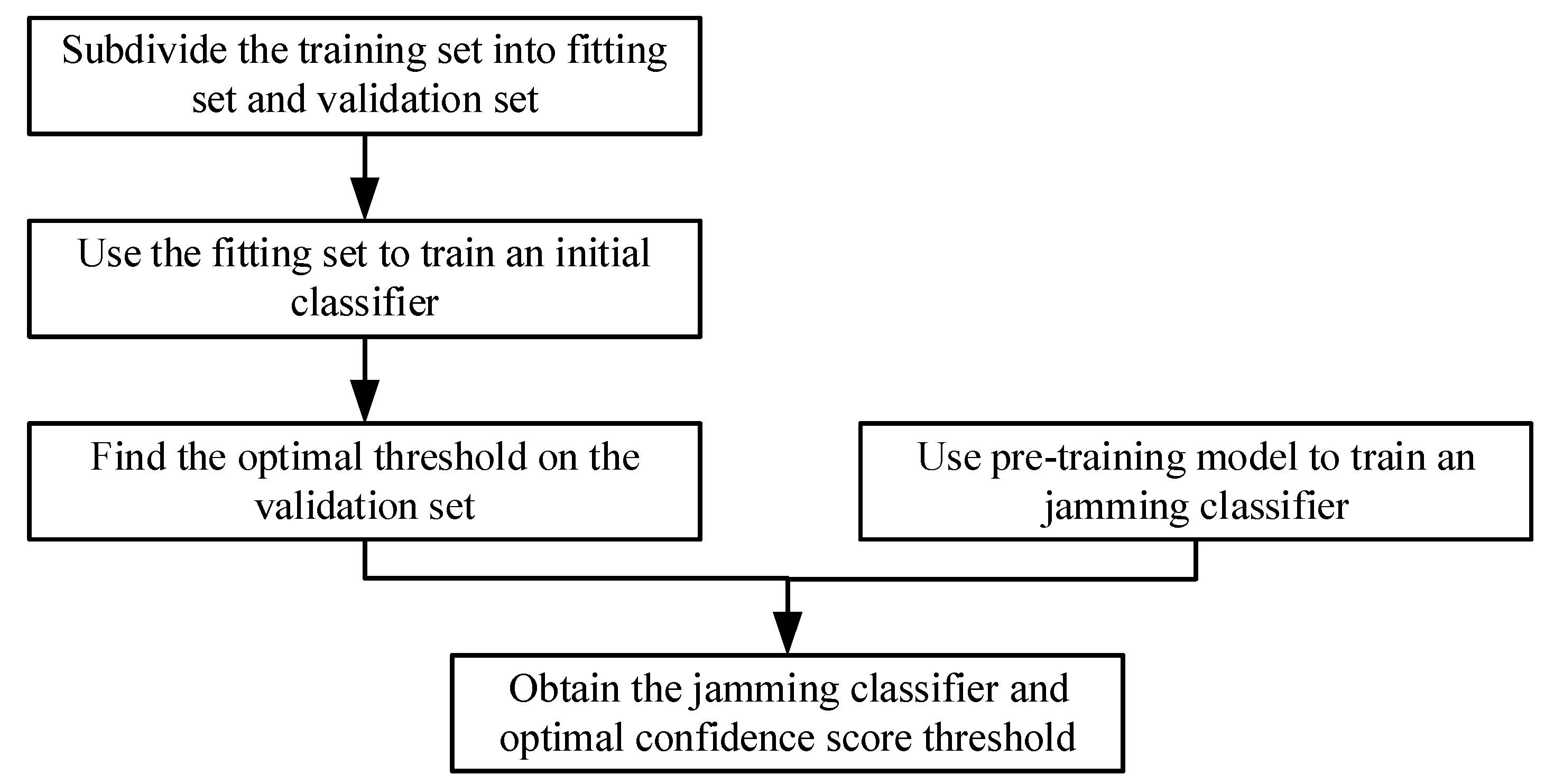
Given that we have no information about unknown jamming in the actual open set environment, the threshold can only be determined using the training set. The training procedure of threshold is described as follows:
First, we need to simulate the open set environment in the training set, so we assume a part of the known jamming categories in the training set as unknown. Here we assume four types of jamming as known and the other four types as unknown.
Second, we subdivide the training set into fitting and validation sets, where all the samples in the fitting set are assumed known jamming, and the validation set includes the assumed known jamming and the assumed unknown jamming. The result of the division is shown in
Figure 8.
Third, we use samples in the fitting set to train an initial classifier, which will be used to train the optimal threshold in step 4.
Fourth, we use the initial classifier obtained in step 3 to train the optimal threshold
in the validation set. The objective function of training the optimal threshold is shown in Equation (5).
where
is the number of assumed known jamming in validation set
,
is the number of assumed unknown jamming in validation set
,
is the confidence score of an assumed known jamming sample,
is the confidence score of an assumed unknown jamming sample,
is the misjudgment penalty weight of the assumed known jamming,
is the misjudgment penalty weight of the assumed unknown jamming,
is the sign function, and
is positive for
and negative for
.
The explanation of Equation (5) is as follows: If a jamming sample is an assumed known one, then we hope that its confidence score is bigger than threshold , so we let be positive as the misjudgment penalty for is smaller than . In the same way, if a jamming sample is an assumed unknown one, then we hope that its confidence score is smaller than threshold , so we let be positive as the misjudgment penalty for is bigger than . Lastly, we obtain the penalty function to be optimized and then minimize it to obtain the optimal threshold by doing this for all samples in the validation set (including those assumed to be known and those assumed to be unknown).
In the actual training process, we choose genetic algorithm (GA) [
32] to optimize the Equation (5).
3.2.4. Training and Testing Process
The training process is shown in
Figure 9. This process consists of two parts. The first part is to obtain confidence score threshold
. We need to subdivide the training set into fitting set
and validation set
. Then, an initial jamming classifier is trained on the fitting set by using the pre-training model, and an optimal confidence score threshold
is found by minimizing the misjudgment penalty function on validation set
. The second part is to train a jamming classifier, which uses the pre-training model to train one jamming classifier on all the jamming training datasets.
The testing process of the OSR model based on the confidence score is shown in
Figure 10. First, the jamming samples to be classified are inputted into the trained jamming classifier to obtain the probability distribution that the jamming samples belong to different known jamming types. Then, the confidence score
of the probability distribution is calculated by using Equation (3). Finally, we judge whether the confidence score
exceeds the optimal threshold
or not. We choose the jamming type with the highest probability value as the output recognition result for
; otherwise, we output it as an unknown jamming type. In the testing process, the time complexity of processing one jamming sample is O(N+2), where N is the number of jamming types in the training set.
3.3. OSR Model Based on OpenMax
The OSR model based on the confidence score needs to simulate the open set scenario and determine the threshold of the confidence score. This approach causes two problems: First, the open set environment simulated by the training set might have a massive deviation from the actual open set environment. Second, because certain unknown jamming might be highly similar to a known jamming class, the probability distribution would be similar to that of some known jamming, causing the confidence score threshold to fail to distinguish between the known and unknown classes. An OpenMax-based OSR model is proposed to solve these problems, which does not require setting any threshold.
3.3.1. Structure of the OSR Model Based on OpenMax
Most jamming classifiers working in a close set environment generate a probability distribution over the known
types of jamming (where
represents the number of jamming types in the training set). When an unknown jamming sample is inputted into the jamming classifier, it is forcibly recognized as one of the
known types of jamming. The OpenMax layer can estimate the probability that the input jamming sample belongs to the unknown jamming by extending the SoftMax layer. This layer changes the output dimension of the jamming classifier from
to
(where 1 represents other unknown jamming types in the testing environment). When an unknown jamming sample is inputted into an open set jamming recognition model based on OpenMax, the output probability distribution of the OpenMax will have a higher probability on the unknown jamming type, thus detecting the unknown jamming type. The structure of the OSR model based on OpenMax is shown in
Figure 11.
The model consists of three parts. The first part is the jamming classifier, the function of which is to train a jamming classifier on the training set by using the pre-training model, extracting the output of the second-last layer of the jamming classifier as the activation vector (the full connection layer before SoftMax). Given that CNN can efficiently extract image features and reflect them on the activation vectors, we can measure the similarity between the input jamming samples by calculating the distance between the activation vectors of the input jamming samples. The second part matches the boundary of known jamming and the Weibull distribution of the known jamming boundary. The function of this part is to match the Weibull distribution of the distance between the input jamming sample and the activation vector boundary of each known jamming. The probability that the input jamming samples do not belong to known jamming can be determined through the Weibull distribution. The third part is to build the OpenMax layer. The function of this part is to create the probability distribution of types based on the Weibull distribution of each jamming type to ensure that the probability that the input jamming sample belongs to an unknown type can be included in the output probability distribution.
3.3.2. Match the Boundary of Known Jamming
The activation vectors extracted by the classifier network from the input jamming samples of the same type will gather together because of the similarity of the jamming samples from the same type. The samples of the different types will form distinct communities in the space of the activation vector because of the variations among the different types of jamming. Moreover, a difference exists between the unknown and the known jamming samples. The unknown jamming type is far from the known jamming type community in the activation vector space. In this work, the center of the activation vector of each known jamming type is the average activation vector. Each known jamming type’s average activation vector is determined by averaging the activation vectors of all samples. The distribution of the jamming samples in the activation vector space is illustrated in
Figure 12. The dimension of the activation vector is
(where
is the number of known jamming types). Here, only two dimensions are taken to intuitively reflect the activation vector’s characteristics.
In
Figure 12, every jamming type has its boundary point, which is far from the average activation vector. The activation vector communities of the known jamming types can be obtained in the activation vector space after the training process. Consequently, if an unknown jamming type is inputted into the classifier during the testing process, an activation vector that is far from all of the jamming activation vector communities can be obtained.
Based on the above principle, when a new jamming sample is inputted, its activation vector can be determined whether it belongs to the jamming type by determining whether it is within the boundary of the known jamming communities.
We use the extreme value theorem [
33] to define the boundary for each type of jamming, which is as follows: Given
samples of identical and independent samples
from an unknown distribution
, the maximum of
n samples
follows the Weibull distribution. The cumulative distribution function (CDF)
of the Weibull distribution is as follows:
where
are the three parameters of the Weibull distribution;
is the maximum value;
is a variable of CDF; and
means the probability that the maximum value
is less than x.
The jamming samples of the same type can be considered from the same distribution and independent of each other. The boundary points of each type of jamming can be considered to be the samples with the farthest distance between the activation vector and the average activation vector. Based on the extreme value theorem, the distance between the activation vector and the average activation vector of each known jamming boundary point follows the Weibull distribution. The boundary of each known jamming can be obtained by matching the Weibull distribution of the boundary point of each known type. This work uses 10 samples, the activation vector of which is farthest from the average activation vector to match the Weibull distribution of the boundary points of every known jamming type. When a new jamming sample is inputted, the distance between the jamming sample activation vector and the average activation vector of each known jamming type is first calculated. Then, the distance is inputted into the Weibull distribution of the boundary points of each type of jamming, and the probability that the boundary distance of each type of jamming is less than that distance is obtained, that is, the probability that the jamming sample is outside the boundary of the corresponding known jamming type (the input jamming sample does not belong to the known jamming type).
3.3.3. Build the OpenMax Layer
The OpenMax layer constructs a probability distribution of class N+1 from the Weibull distribution at the boundary of known jamming types. Accordingly, the probability distribution of the output contains the probability that the input jamming samples are of unknown jamming types.
The building process of the OpenMax layer is shown in Algorithm 1. First, we extract the activation vector
of the testing jamming sample
. Next, the probability
that the testing jamming samples belong to each type of known jamming is calculated using the boundaries of the known jamming matched by Weibull distribution (where
denotes the probability that test jamming sample
belongs to class
of known jamming and is derived from the probability that 1-Test sample does not belong to class
of known jamming). Then, the new activation vector is redefined. The length of the new activation vector changes from
to
. The new activation vector contains two parts. The first part is the activation value of the test samples for known jamming of class
, which includes
activation values
. This value is obtained by performing a dot product between the original activation vector and the probability that a testing sample belongs to each of the known jamming types. The second part is the activation value of the testing jamming sample on the unknown jamming class, which is
. This value is obtained by performing a dot product first between the original activation value and the probability that a testing sample does not belong to each of the known jamming types and then summing up the results. Finally, the probability distribution of the OpenMax output is obtained based on the new activation vector. The probability distribution of the output includes the probability that the test jamming samples belong to all types of known jamming and the probability that the test jamming samples belong to unknown jamming. The final output chooses the type with the highest probability as the recognition result. OpenMax changes the output
dimensions of the open set jamming recognition model from
dimensions by estimating the probability that the testing jamming samples belong to the unknown jamming. When the unknown jamming samples are inputted into the open set jamming recognition model based on OpenMax, the probability distribution of the OpenMax output has a higher probability on the unknown jamming type, thus distinguishing the unknown jamming type. Furthermore, the OpenMax-based OSR model does not need to simulate the open set environment to set thresholds compared with a confidence score-based OSR model. The algorithm of OpenMax has the time complexity of O(2N+5). The time complexity of OpenMax-based model is in the same order of magnitude as that of confidence score-based model.
| Algorithm 1. OpenMax layer building algorithm |
| OpenMax: Estimate the probability that the input jamming is an unknown class |
Input: Activation vectors of testing samples;
Average activation vector for known jamming typesand Weibull distribution parameters of boundary points;
1 for
2
3 end
4 redefinition activation vector
5 define the unknown part of the activation vector
6. Probability distribution generated by OpenMax:
7. recognition result: y* = argmaxP(y = j|x) |
3.3.4. Training and Testing Process
The training and testing processes of the model based on OpenMax is shown in
Figure 13. The training process is described as follows:
First, a pre-training model is used to train a jamming classifier on the jamming training set. Then, the activation vectors of all known jamming samples are extracted, and the average activation vectors of every type of known jamming are calculated. Finally, the Weibull distribution is used to match the boundary of each type of known jamming. The testing process is described as follows: First, the jamming samples to be recognized are inputted into the jamming classifier, and the activation vectors of the jamming samples are extracted. Then, an OpenMax layer is constructed based on the activation vectors of the jamming samples and the Weibull distribution of each known jamming boundary. Finally, the highest probability type in the probability distribution of the OpenMax output is selected as the output of the recognition results.
4. Simulation and Analysis
This section describes in detail the experimental parameters and results, which includes the simulation results of the jamming signal, the parameters of pre-training networks, and the performance of the OSR proposed in this work. Several experiments are implemented to verify the performance and robustness of the two OSR models we proposed. These experiments include the improvement of recognition performance after L1 and L2 regularization, the analysis of average accuracy in open set jamming recognition with and without the number of unknown types of jamming fixed, and the robustness analysis of the two OSR models. Experiments show that both models perform effectively in complex open set environments (lower JNR and more unknown types) and can be used in the jamming recognition part of radars in practice.
4.1. Jamming Signal Datasets
Eleven types of jamming signal have been simulated in this work, and their time–frequency images have been obtained by STFT. The parameters of the time–frequency images are as follows: the sampling frequency of the jamming signal is 400
, and the sampling time is
. The window function is the Hamming window, the length of which is 512. The jamming to noise ratio (INR) is −5–10 dB. The size of time–frequency images is
. The time–frequency images of the 11 types of jamming signal are shown in
Figure 14, and the specific parameters of each jamming signal are illustrated in
Table 1.
4.2. Parameters of Pre-Training Networks
Due to the gradient elimination problem of deep network, if the number of layers of the network continues to increase, then the recognition performance of the model will degrade after increasing to a certain number of layers. The pre-training networks in this work will use the residual network structure [
34] to address this problem. A batch normalization processing layer [
35] is added to improve the training speed of the residual module and prevent it from overfitting after the convolution layer of the classical residual module.
We designed a pre-training network based on the improved residual module. The pre-training network consists of four parts. The first part is a convolution layer that has 64 convolution kernels with the size of
. The second part includes four residual module groups [
35], each of which has a convolution kernel size of 5 × 5; the number of residual modules is 3, 4, 6, 3, and the number of convolution kernels is 32, 64, 64, 128, respectively. The third part is a full connection layer. The fourth part is a SoftMax classification layer. The activation functions in the convolution layer and the residual module are the Rectified Linear Units [
36]. The parameters of the pre-training networks are shown in
Table 2.
4.3. Regularization Analysis of Network Parameter
The recognition performance of the two OSR models with and without regularization will be analyzed below. Regularization [
37] is a method of preventing network models from overfitting by restricting the objective function. The two commonly used regularization methods are L1 and L2 regularization. Three groups of experiments are performed on two open set jamming recognition models. The first group is that two open set jamming recognition models do not use regularization, and the second group is that two open set jamming recognition models use L1 regularization. The third group is that two open set jamming recognition models use L2 regularization. The jamming data used in this experiment are 11 active radar jamming signals introduced in
Section 2. Every jamming in the training set of each experiment consists of 100 samples, and that in the test set involves 100 samples. Both models use the same training and test sets for training and testing.
The accuracy, average precision, average recall, and average F-score [
38] of the two open set jamming recognition models are calculated during the testing process. The recognition performance results of the two open set jamming recognition models before and after regularization are shown in
Table 3 and
Table 4, respectively. In
Table 3, the regularization improves the accuracy of the open set jamming recognition model based on the confidence score by about 2%, and the recognition performance of the L2 regularization is better. In
Table 4, the regularization improves the accuracy of the OpenMax-based open set jamming recognition model by about 3%, of which L2 improves the recognition performance better. It can be proved that both the confidence score-based and OpenMax-based OSR models can obtain excellent performance in open set environment after L2 regularization, of which the accuracy is as high as 90%.
4.4. Recognition Performance Analysis of OSR
Two open set validation experiments are designed to verify the recognition effect of the OSR model on unknown jamming, which are the performance of two OSR models with the number of unknown jamming types fixed and with the increase of unknown jamming types. In these experiments, we can find the models’ ability to distinguish unknown jamming signals.
4.4.1. Experiment with the Number of Unknown Jamming Fixed
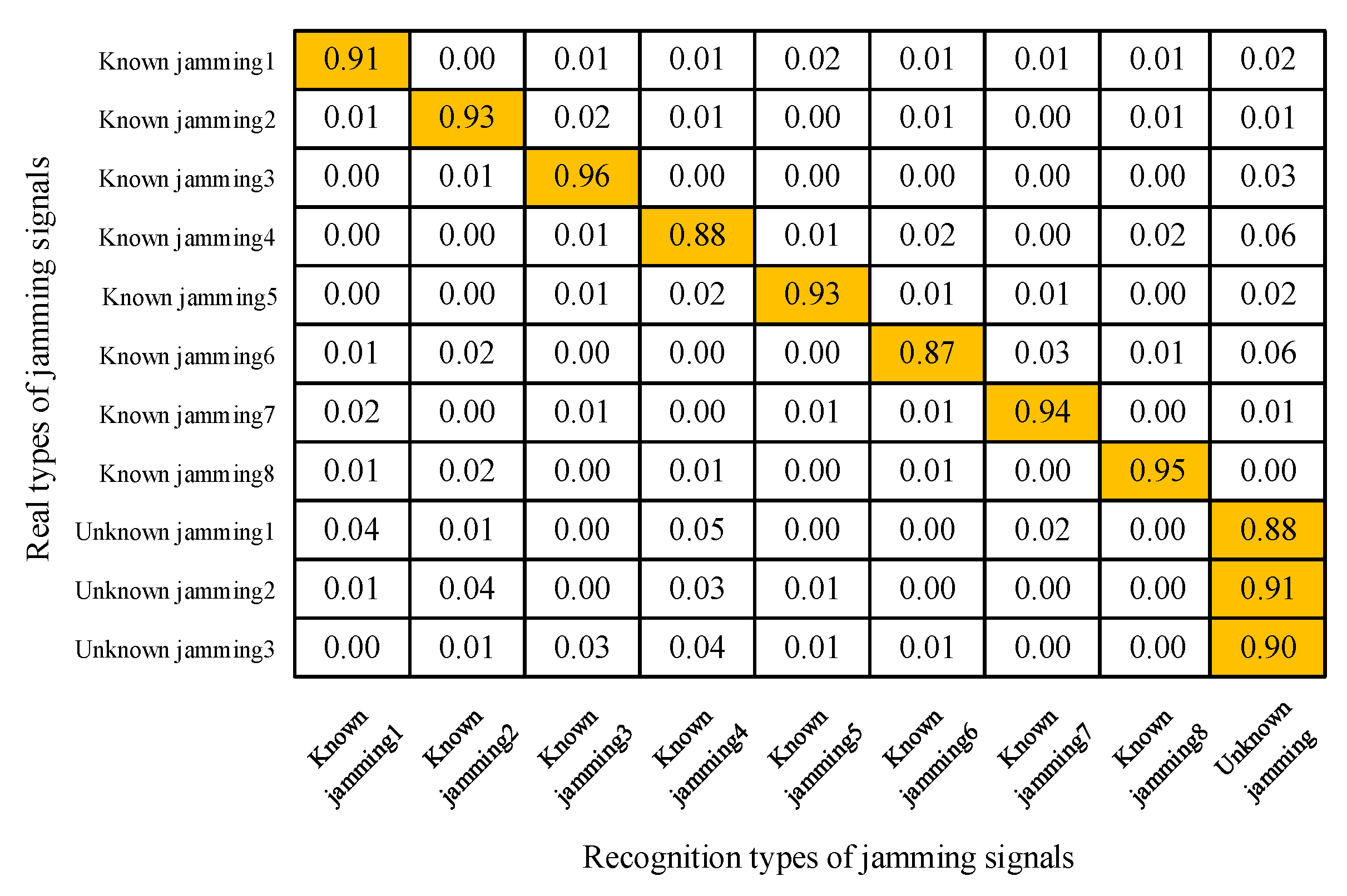
This experiment set up eight known jamming types, namely, noise AM jamming, noise FM jamming, RF noise jamming, RGPO jamming, VGPO jamming, SMSP jamming, C&I jamming, and ISRJ, and three unknown jamming types, including RGPO & noise AM jamming, RGPO & noise FM jamming, and RGPO & RF noise jamming. The jamming training set contains eight known jamming, and the jamming testing set contains eight known and three unknown jamming. Existing closed-set jamming recognition models (CNN jamming recognition model), the open set jamming recognition model based on confidence score, and the open set jamming recognition model based on OpenMax are trained on the jamming training set and tested on the testing set. The recognition result of the first experiment is shown in
Figure 15,
Figure 16 and
Figure 17.
Figure 15 shows the confusion matrix of the recognition result of the CNN model based on the close set.
Figure 16 shows the confusion matrix of the recognition result of the model based on the confidence score.
Figure 17 shows the confusion matrix of the recognition result of the model based on OpenMax.
In
Figure 15, the CNN model based on a close set obtains good results on the recognition of known jamming types, and the average accuracy rate of the known types is 89.63%. However, this model does not efficiently perform if the samples belong to an unknown type and are recognized as one of the known jamming types. This notion indicates that the existing close set recognition model is not competent for jamming recognition in open set scenarios.
Figure 16 shows that the OSR model based on the confidence score has a high average accuracy rate not only on the known jamming samples (88.5%) but also on the unknown jamming samples (80.33%). In
Figure 17, the OSR model based on OpenMax has better recognition results, whose average accuracy rate of known jamming samples is 92.13%; that of unknown jamming samples is 89.67%. It is proven in this experiment that both the confidence score-based and OpenMax-based OSR models have the ability to distinguish the unknown type of jamming signals.
4.4.2. Experiment with the Unknown Jamming Type Increasing
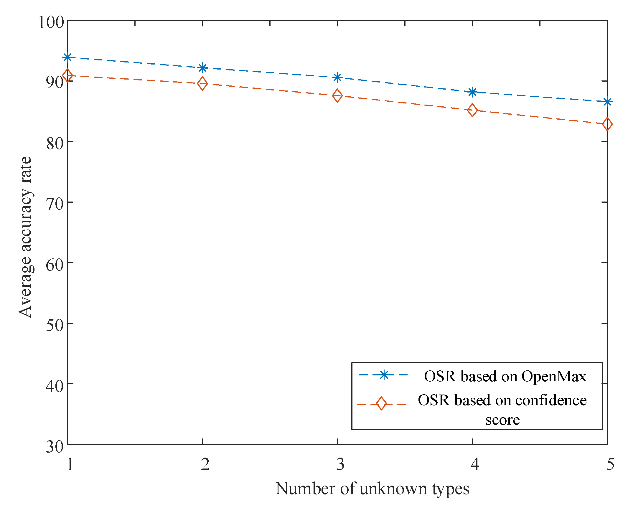
The recognition performance of the two models will be tested in different open set environments to further verify the two jamming OSR models. Five open set jamming testing environments are set up. The numbers of unknown jamming types in open set jamming testing environments are one class, two classes, three classes, four classes, and five classes. The recognition results of two OSR models in different open set testing environments are shown in
Figure 18. The recognition average accuracy rate of the OSR model based on the confidence score and the OSR model based on OpenMax gradually decreases with the number of unknown jamming types increasing in the open set jamming testing environment. Moreover, the average accuracy of these two models remains as high as nearly 85%, even though the number of unknown types is five. The OSR model based on OpenMax has better recognition performance than the open set jamming recognition model based on confidence scores under different open set jamming testing environments. It can be proved in this experiment that the two OSR models have good generalization performance in the open set environment with many unknown jamming types and they can maintain basic recognition ability (The average accuracy is above 85%) even though there are nearly 50% unknown jamming types (5 of the 11 jamming types are unknown) in the open set environment.
4.5. Robustness Analysis of OSR
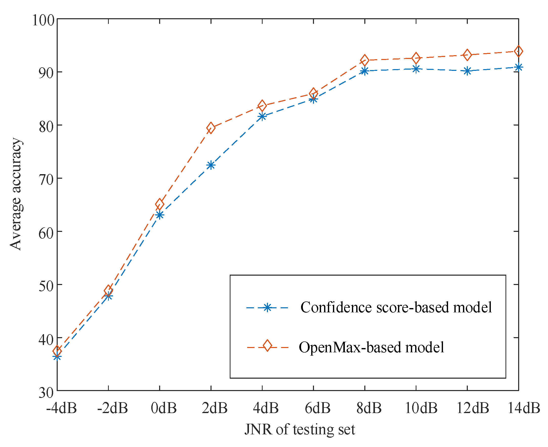
To verify the stability of the jamming OSR model proposed in this work under different jamming-to-noise ratios (JNRs), we also perform an experiment to test the recognition performance of the models under different JNRs. In this experiment, the number of jamming samples in the training set is 100. The JNRs of the testing set are −4, −2, 0, 2, 4, 6, 8, 10, 12, and 14 dB.
The accuracy of the two OSR models under different JNRs is shown in
Figure 19. The accuracy of the OSR model based on the confidence score and OpenMax is about 60% when the JNR is 0 dB. The recognition accuracy of the two OSR models increases with the increase in the JNR. The accuracy of the two models is basically the same when the JNR is lower than 0 dB. When the JNR rises to 4 dB, the accuracy of the model based on OpenMax is 10% higher than that of the model based on the confidence score. The accuracy of the two models is about 90% when the JNR reaches 8 dB. Moreover, the accuracy of these two models remains approximately 90% with the increase in the JNR. Based on the results of
Figure 19, the performance of the two OSR models differs slightly under different JNRs, with that of the open set jamming recognition model based on OpenMax slightly higher. Although the recognition performance will inevitably decline with the reduction of JNR, we can see from
Figure 19 that when the JNR is more than 8dB, both models have higher average accuracy, which is as high as 90%.
5. Conclusions
When the existing radar jamming recognition models are tested in an open test environment with unknown jamming, the existing jamming recognition models will recognize the unknown jamming as one known type in the training jamming library. This work discusses the jamming recognition models in open set scenarios to solve the problem existing in the jamming recognition methods of radar.
In this work, the jamming recognition of radar in open set scenarios is studied, and two solutions for open set jamming scenarios are presented, which are based on the confidence score and OpenMax OSR model. The OSR model based on the confidence score generates the probability distribution of the input jamming signals over known jamming types through the jamming classifier. Then, the confidence score of the probability distribution is calculated to determine whether the result of the jamming recognition is reliable. If the finding is reliable, then the result of the jamming classifier is outputted; otherwise, the output jamming is unknown. The OSR model based on OpenMax first extracts the activation vector from the input jamming signal to the jamming classifier and then constructs an OpenMax layer containing the probability that the input jamming sample is an unknown jamming type based on the activation vector of the jamming sample and the Weibull distribution of each known jamming boundary. Finally, the model selects the type with the highest probability in the probability distribution of the OpenMax output as the output of the recognition result.
After verification, the two OSR models can perform well in the open set jamming environment. The average accuracy is as high as 90% after regularization, and the OSR performance remains good with the increase of the unknown types in the testing set. Meanwhile, the two models also have good robustness. Thus, the unknown jamming types can be detected in a low JNR. The two models proposed in this paper need to be trained before the actual test. Among them, the training set is used to obtain the threshold in the confidence score-based model during the training process, while the boundary of Weibull distribution should be matched in the OpenMax-based model in advance. In the test, the algorithms in the two models have the same magnitude of time complexity.
Through the two open set jamming recognition models proposed in this paper, the radar can be competent for the task of correctly identifying the type of jamming signal in the open electromagnetic environment. This makes it easier for the radar anti-jamming system to implement anti-jamming measures for the specific type of jamming. The concept and technology of OSR can not only be used in radar jamming recognition, but also can be used in the recognition and positioning of civil radars and satellites, such as remote sensing intelligent interpretation, identity authentication, and pattern classification. However, current studies on OSR are not able to properly classify samples of unknown types into specific categories. Further studies can focus on how to solve this problem.


