Review

A Survey of Computer Vision Techniques for Forest Characterization and Carbon Monitoring Tasks

1
Skolkovo Institute of Science and Technology, Bolshoy Boulevard 30, bld. 1, 121205 Moscow, Russia
2
Institute of Information Technology and Data Science, Irkutsk National Research Technical University, 664074 Irkutsk, Russia
3
Federal Research Center “Computer Science and Control”, Russian Academy of Sciences, Vavilov Str. 44/2, 119333 Moscow, Russia
4
Public Joint-Stock Company (PJSC) Sberbank of Russia, 117312 Moscow, Russia
5
Marchuk Institute of Numerical Mathematics, Russian Academy of Science, 119333 Moscow, Russia
6
Autonomous Non-Profit Organization Artificial Intelligence Research Institute (AIRI), 105064 Moscow, Russia
*
Author to whom correspondence should be addressed.
Remote Sens. 2022, 14(22), 5861; https://doi.org/10.3390/rs14225861
Submission received: 28 October 2022 / Revised: 15 November 2022 / Accepted: 16 November 2022 / Published: 19 November 2022

Abstract

:
Estimation of terrestrial carbon balance is one of the key tasks in the understanding and prognosis of climate change impacts and the development of tools and policies according to carbon mitigation and adaptation strategies. Forest ecosystems are one of the major pools of carbon stocks affected by controversial processes influencing carbon stability. Therefore, monitoring forest ecosystems is a key to proper inventory management of resources and planning their sustainable use. In this survey, we discuss which computer vision techniques are applicable to the most important aspects of forest management actions, considering the wide availability of remote sensing (RS) data of different resolutions based both on satellite and unmanned aerial vehicle (UAV) observations. Our analysis applies to the most occurring tasks such as estimation of forest areas, tree species classification, and estimation of forest resources. Through the survey, we also provide a necessary technical background with a description of suitable data sources, algorithms’ descriptions, and corresponding metrics for their evaluation. The implementation of the provided techniques into routine workflows is a significant step toward the development of systems of continuous actualization of forest data, including real-time monitoring. It is crucial for diverse purposes on both local and global scales. Among the most important are the implementation of improved forest management strategies and actions, carbon offset projects, and enhancement of the prediction accuracy of system changes under different land-use and climate scenarios.

Graphical Abstract

1. Introduction

Climate change adaptation and mitigation policy make the development tools for estimation and monitoring flows of greenhouse gases (GHG) relevant. Such accounting of ecosystem balances helps to understand and alter trends of GHG emissions. As for now, a more accurate inventory of carbon stocks and sources is a subject of ongoing discussions. It aims at reducing the uncertainty of carbon balance estimations and their prognosis in different economic and climate change scenarios. It includes clarifying user and social choices in the decision-making process. Improvements of on-site measurement techniques along with scaling of the accounting systems (models) have lead to a more detailed level for a better understanding of the carbon cycle [1,2,3,4,5].
Among a variety of natural and artificial ecosystems, forests show mostly predominant sequestration of carbon from the atmosphere. Mostly negative net GHG fluxes characterize territories under forests; as a result, gross carbon removals exceeded gross emissions around the world [6]. At the same time, in the presence of disturbances, CO2 emission increases due to a release of the carbon retained in the ecosystem [7]. The list of main disturbing events includes, in general, the change of forests to other land use types, the use of forest resources for materials and energy due to harvesting, the occurrence of fires, fall-outs, change of water regimes, change of the community structure due to pathogens and invasion outbreaks, and development of deadwood. Those are considered to be managed to maintain sustainable long-term use of natural resources and receive climate benefits [8,9].
As for now, most of the forest monitoring, management, and planning needs at different spatio-temporal scales can be covered by the use of remote sensing data (RS) [10,11,12,13]. Among these tasks are estimation of forest structural and functional diversity, productivity assessment, catching the degradation processes and their patterns, deforestation detection and analysis, and others. RS data include both orbital and unmanned aerial vehicle (UAV) observations. For instance, the Sentinel-2 mission can provide multispectral information, while the Global Ecosystem Dynamics Investigation (GEDI) mission [14] provides laser measurements. Both of them can be used for carbon cycle studies. The detailed information about orbital missions is presented in Section 3. To date, many countries have already included remotely sensed earth observations in their forest inventories within national procedures. However, only 10 to 30% of this information, depending on the data type (satellite images and airborne photography, respectively), is considered for inventory completion [15]. Such data are, in fact, the primary source of information for observing large territories or locations that are hard to access. Currently, there is a strong demand for detailed information about the sources, sinks, and transport of CO2, as well as about their change under different influencing factors [16,17]. It can be expected that the broad involvement of the RS data into routine protocols of monitoring of natural and managed ecosystems is merely the matter of time [18]. Thus, techniques for analyzing RS data are also under development, while their operational integration is an essential part of system knowledge progress [12].
We can notice the steady development of machine and deep learning, improvement of computational resources, along with public availability of the Earth nearly big data (diverse remotely sensed records obtained by a plethora of sensors at various spatial and temporal resolutions). It can be used for the tasks related to the tackling of land-atmosphere interactions, in particular, applicable to the forest areas [19]. In this regard, machine learning algorithms and computer vision (CV) are of great practical and scientific interest. In what follows, by a CV we mean all methods for image processing, and, specifically, classical machine learning methods and deep learning methods based on neural networks. CV techniques are recognized as a powerful tool capable of capturing information from the data of different domains, both photo, and video, and of handling target tasks at different scales. CV algorithms combine the usability and potential for automatization, determined by transparent algorithms’ pipelines. By using the standardized list of metrics, we can tune the performance and evaluate the model quality. At the same time, it is worth noticing the capability of CV algorithms to integrate expert knowledge during the training procedure [20,21]. The sufficient advantage of this group of modeling and analysis methods is its potential to overcome the main limitations related to the lack or incompleteness of the data [22,23].
There are a number of surveys covering different aspects of forestry studies published in recent years. The number of publications about RS and forestry tasks has increased twice during the last decade, while the number of references to machine learning applications has increased almost tenfold (see Section 2). Particular forest properties estimation, such as aboveground forest biomass, has been surveyed in [24]. It was summarized that RS in forest aboveground biomass estimation is a perspective alternative to conventional ground-based approaches. Since the publication of this survey publishing in 2016, new RS data sources have become available and widely used, and there has also been a drastic rise in machine learning and deep learning, and their implementation in environmental studies. The following surveys were focused on carbon stocks and carbon cycle, highlighting the most commonly used RS data sources [25,26]. In [12], another forestry problem was observed, namely, forest degradation focused on the used data and its important properties. In turn, in the current survey, we aggregated information from recent studies related mostly to the CV algorithms application for the exact forestry problems: forest mask, tree species, and forest resources estimation. We chose exactly these forest properties, as they are one of the core components for forestry analysis and have a significant impact on carbon monitoring and various environmental tasks [25]. Currently, there are a lot of data and algorithms that allow one to solve numerous problems, including those related to obtaining forest characteristics based on satellite data. Due to the wide variety of data sources, their specifics, and algorithms, it is difficult for a novice researcher to find a suitable approach that combines the use of certain data and algorithms that would give a good result shortly. In order to have an understanding of the available data and algorithms that best solve the particular problem, taking into account the specifics of the problem being solved, we provide this survey. It covers the most popular data sources and widely used methods, as they are both of high value for accurate RS solutions. It will allow researchers to effectively select a set of suitable algorithms and data sources that will solve a specific problem.

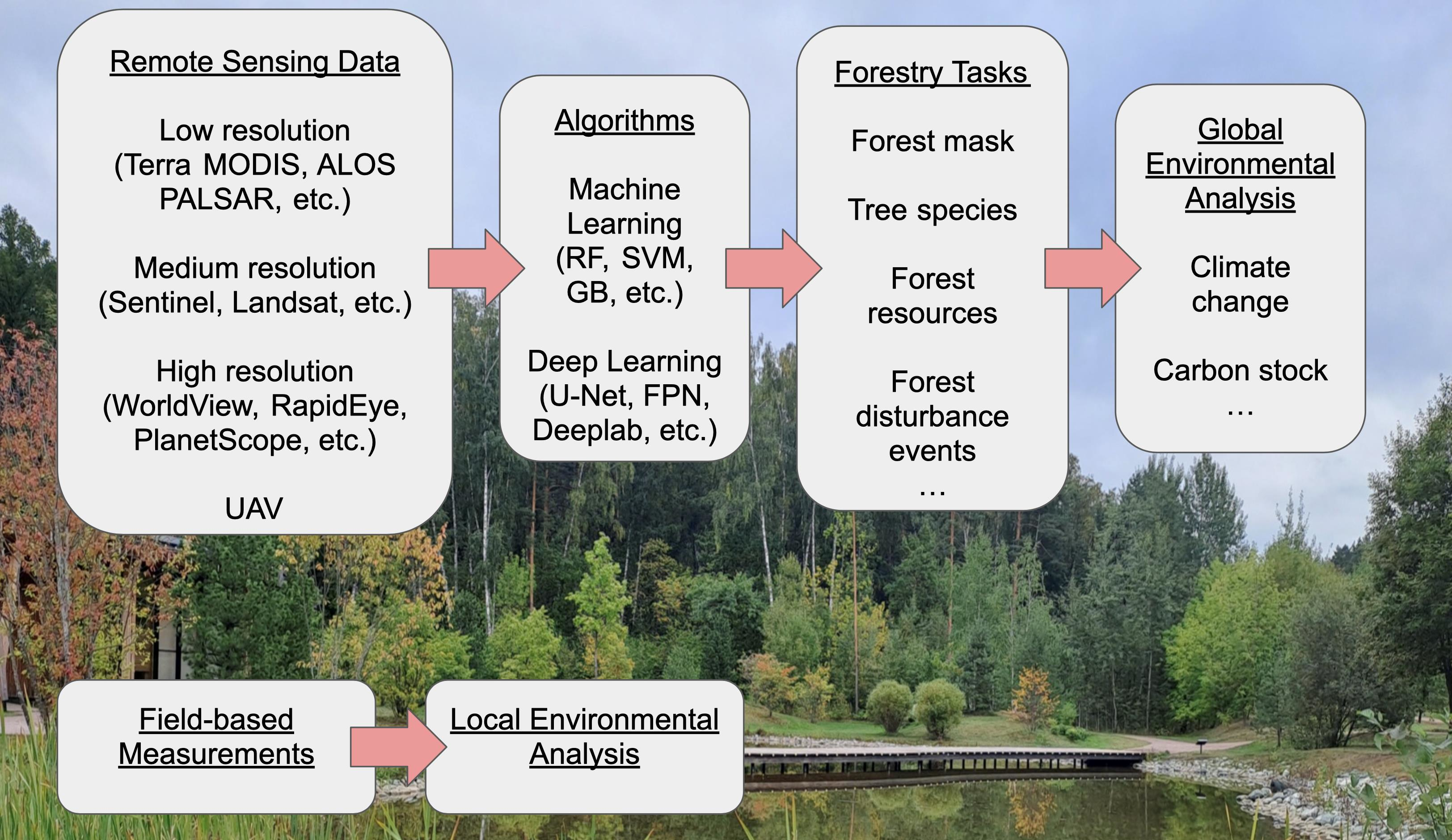
2. Review Methodology

Interest in remote sensing of the environment, namely, forest characteristics estimation, has been constantly growing during the last decade, as shown in Figure 1. To collect year wise statistics, we used two sets of words as keywords in the “article title, abstract, and keywords” in the Scopus database search system. The first set of words specifies remote sensing research domain, including words “remote sensing”, “UAV”, and certain widely used satellites names. The second set of words concretizes a specific forestry properties and tasks such as “tree mapping”, “growing stock volume”, “age”, “forest species”, etc. The “AND” Boolean operator united these two sets of words, while within each set, the “OR” operator was applied. The search resulted in over 18,000 publications from 2011 to 2021 year. The search excluded subject areas such as medicine, social science, etc. In Figure 1, “ML + Remote sensing” refers to the intersection of the previous search results with a set of words specifying artificial intelligence algorithms such as “machine learning”, “deep learning”, “neural networks”, and names of widely used algorithms. The search resulted in over 2200 documents from 2011 to 2021. There is a solid growth in the number of publications considering artificial intelligence since 2015 year. Comparing the search results for machine learning applications for different RS forest tasks, we can notice that the most frequently encountered task is forest resources estimation such as aboveground biomass, growing stock, and standing volume (over 900 documents from 2011 to 2021 years). Forest species classification using artificial intelligence ranks second in the search results (over 800 documents). Classical machine learning algorithms (such as Random forest, Gradient boosting, etc.) occur three times as often as deep learning algorithms. Among RS data, Landsat is referred with machine learning algorithms in over 400 publications. Sentinel data was mentioned in over 340 papers for forest tasks using machine learning techniques, while WorldView data were mentioned in over 100 publications. The detailed information about data sources and tasks is presented below.
The literature analysis is performed using recently published studies from peer-reviewed journals included in the Scopus scientific database. The Google Scholar database additionally supported the search. Due to the rapid development of the data science discipline, the survey timeline was limited, starting from the year 2017 to 2022. An exception is applied to the research that is fundamental or was a pioneer to the topic, according to the citation level and earlier years of publishing. For each discussed topic, we used relevant keywords, for example, “aboveground biomass” and “forestry” and “remote sensing”. The results of such requests were compared with search query after adding the words “computer vision”, which was not obligatory used firstly because of the frequent association of the phrase with neural networks only. Then, the search results were manually examined with and without sorting by the citation level, and relevant works were chosen for detailed analysis. Zero citations were acceptable in the case of specific (influential) journals relevant to research topics of earth science, environmental science, and environmental monitoring and 2022 as the year of publishing. However, to catch the general context, for the most part, publications with more than 20 citations were considered. Our search was limited by the keywords’ combinations in the title and abstract, the final publishing stage, and English language. We mainly considered research articles to make conclusions about the applicability and efficiency of the algorithms. However, our analysis also includes relevant comprehensive reviews’ references providing general trend analysis within the topic of climate change mitigation actions and data sources.

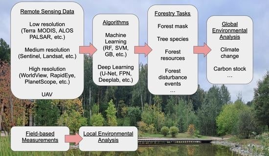
3. Remote Sensing Data and Spectral Indices for Forest Analysis

3.1. Sources of Remote Sensing Data

An essential part of developing a vegetation analysis methodology is the informed choice of one or another data source. We refer the reader to the latest extensive surveys dedicated to the descriptions of the common RS platforms and sensor combinations applied to the problem of vegetation analysis [12,13,28,29], while noting that this is a rapidly evolving field. In the present study, we provide the list of main characteristics of the currently most commonly used instruments of particular importance for forest-related tasks at different scales (Table 1).
When choosing a data source for research, various details are taken into account: data availability, survey repeatability, spatial resolution, sensor type, sensor specifications, range of spectral channels, etc. Describing RS data, one can distinguish different spatial, temporal and spectral resolution, while the “spatial” meaning is the most frequent case. In the case of spatial resolution, we refer to the precision classification as coarse (low), medium and fine (high) [25,30]. Thus, low resolution corresponds to the data of pixel size of more than 30 m per pixel, medium resolution corresponds to the data of pixel size from 10 to 30 m, and high resolution, to the size of less than 5 m.
Many RS missions are capable of providing up-to-date and diverse information about the object or phenomenon under consideration. Each approach has advantages and limitations, determined by the detection conditions and the ratio between spatial resolution, revisiting time, or cost. Active sensors such as radar are independent of the weather conditions and do not rely on the sun as a source of illumination, and so can provide the data regardless of the day or night conditions. On the contrary, passive multispectral and hyperspectral sensors require solar radiation. Additionally, the coarser the image obtained from the satellite, the more often it is taken. To combine the frequency of low-resolution imaging with more details of the other available data or to restore the information that was lost due to unsuitable conditions, different machine learning fusion techniques were implemented [19].
One can choose the most appropriate satellite data for required time and territory. The number of available bands in different satellites may vary. It is possible to use all bands available in the chosen satellite, select, or combine (to obtain spectral indices) some of them. A special case of the auxiliary use is the panchromatic channel. Due to its wide band, it gains more light; therefore, it has higher spatial resolution. It makes it possible to adjust the resolution of satellite imagery through pan-sharpening techniques [45].
One of the advantages of platform-distributed RS data is their availability and easy-to-use web and scripting interfaces for collecting the data by end-users. They can be downloaded, free of charge or for payment, from data-aggregating platforms, provided raw data, as well as pre-processed or converted into various valuable derivatives such as spectral indices or reflectance bottom of the atmosphere (BOA). This allows the user to generate sets of images for efficient training of machine learning algorithms for different regions and relevant dates for the study. For exploring resources and performance capabilities, we refer the reader to, e.g., Level-1 and Atmosphere Archive & Distribution System Distributed Active Archive Center (LAADS DAAC) Tools and Services collection (https://ladsweb.modaps.eosdis.nasa.gov/tools-and-services/ (accessed on 20 October 2022)), Copernicus Open Access Hub (https://scihub.copernicus.eu (accessed on 20 October 2022)), the Planet Platform (https://www.planet.com/products/platform/ (accessed on 20 October 2022)).

3.2. Popular Spectral Indices Applied for Forest Monitoring Research

Remote sensing data are rich in information, and in the case of multispectral sources, separate bands can be mathematically transformed and combined. Such composites, namely spectral indices, can be used to catch specific patterns necessary for the most common tasks of forest carbon monitoring. Among these tasks are forest area estimation, tree stand composition classification, change or anomaly detection, and others that will be covered further in the following sections.
There are dozens of different spectral indices, and many of them have different modifications [29,46]. Here, we discuss some of the most frequently utilized. One of the most popular spectral indices is the group of vegetation indices, led by the Normalized Difference Vegetation Index (NDVI), based on the near-infrared (NIR) and red reflectance bands. NDVI has derivatives, one of which is the Vegetation Condition Index (VCI), based on the minimum and maximum values of the NDVI for a given period. For the study of atmospheric effects, the Atmospherically Resistant Vegetation Index (ARVI) can be used. Although NDVI is a commonly used choice to analyze vegetation cover, it is affected by a saturation problem for densely forested areas [47]. The main reason is that if there is a total leaves cover in the high vegetation period (peak of the vegetation period), the leaves are unable to absorb red light, so the reflectance of red light will increase. Moreover, the intensity of NIR will also increase. According to Equation (1), the calculated NDVI will be underestimated. To address the saturation problem, the Enhanced Vegetation Index (EVI) can be used. It is more accurate in areas with high vegetation and considers both soil and atmospheric effects. Another possible choice for densely forested areas is indices based on a Red-edge spectral band: Normalized Difference Red-edge (NDRE), the Modified Simple Ratio (MSR) Red-edge index, and Chlorophyll Index (CI) Red-edge. However, only some satellites have sensors for Red-edge measurements. The Red-edge band is available, for instance, in the satellite systems such as Sentinel-2, WorldView-2 and 3, and RapidEye.
N D V I = N I R R e d N I R + R e d
N D R E = N I R R e d E d g e N I R + R e d E d g e
where NIR is the near-infrared spectral band, Red is the red spectral band, and RedEdge is the red-edge spectral band.
V C I = N D V I i , p , j N D V I m i n i , p , j N D V I m a x i , p , j + N D V I m i n i , p , j
where i is the pixel, p is the period, j is the year.
A R V I = N I R 1 × ( R e d B l u e ) N I R + 1 × ( R e d B l u e )
where Blue is the blue spectral band.
E V I = 2.5 × ( N I R R e d ) 6 × R e d 7.5 × B l u e + 1
C I R e d E d g e = N I R R e d E d g e 1
M S R R e d E d g e = N I R / R e d E d g e 1 N I R / R e d E d g e + 1
The aforementioned indices are widely used as input data (separately and along with initial bands) to detect the vegetation cover among other different land cover types [48], to distinguish between different plant species [49], to evaluate plant target characteristics such as productivity and mortality [50,51], or to detect insect defoliation [52].
In the field of forest monitoring, one of the most relevant topics is the fire occurrence and spread detection and mitigation [53]. Thus, in addition to described indices, other spectral combinations, mostly based on short-wave infrared reflectance (SWIR), are of common use. For example, one can distinguish the Normalized Burn Ratio (NBR) and derivative Normalized Burn Ratio Thermal (NBRT), Burned Area Index (BAI) for the purposes of the assessment of fire severity and burn area detection [54].
N B R = N I R S W I R N I R + S W I R
where SWIR is the shortwave infrared band.
N B R T = N I R S W I R × T I R N I R + S W I R × T I R
where TIR is the thermal band.
B A I = 1 ( 0.1 + R e d ) 2 + ( 0.06 + N I R ) 2
To consider environmental characteristics and to use it as background for terrestrial and aquatic or coastal forest ecosystems, the following indices are used in addition: Soil Adjusted Vegetation Index (SAVI) allowing us to correct soil brightness [55], the Normalized Difference Water Index (NDWI), also known as the Land Surface Water Index (LSWI), and the Normalized Difference Moisture Index (NDMI) [55,56]. Such indices are also employed to track damages other than fire such as, e.g., pathogen outbreaks [57].
S A V I = ( ( N I R R e d ) × ( 1 + L ) N I R + R e d + L
where L is the soil factor, ranging from 0 to 1, which corresponds to dense vegetation and no vegetation, respectively, while 0.5 is considered default for the most land cover types.
N D W I / L S W I / N D M I = N I R S W I R N I R + S W I R
The use of spectral indices has certain limitations that should be taken into account. Such indices are applicable for the work with RS data in general and include atmospheric effect, the possibility of significant difference between index values in case of different data sources [58], season dependence, in complete accordance with the objects’ features [59]. However, spectral indices provide a valuable source of information with careful pre-processing including appropriate atmospheric correction according to the data source, topographic correction, and understanding the uncertainties along with the availability of the actual measurements (label data). Depending on the goals and study object characteristics, new indices can be proposed based on the previously not used band combination sequences [60]. For the time series, index pattern derivatives can be used such as standard deviation, kurtosis, and skewness [50]. For the recognition and modeling tasks, indices are usually used in combination with each other. Hyperspectral data can also be aggregated into the indices [61].

4. Computer Vision Algorithms

In this section, we describe widely useful supervised algorithms for RS data, in particular, for forest tasks. We discuss both classical machine learning and deep learning algorithms with their specifics, learning process details, and intuition behind them.
Semantic segmentation is a machine-learning problem for which the algorithm learns to determine the class of each pixel using training samples. A feature description characterizes each target object. There is a matching between the input image pixels and ground truth image pixels, which is supposed to be a mask of a perfectly segmented image. The model is aimed at reducing the difference between the prediction and reference markup according to a given quality metric. For instance, in the case of forest mapping, two classes are considered: the forest cover and the areas without forest. Below, we describe the specifics and differences between the classical machine learning algorithms and the DL methods, schematically shown in Figure 2. Although for CNN algorithms, task definition as a semantic segmentation is more conventional; for classical ML approaches, the task is usually defined as a pixel-oriented classification or regression. It means that CNNs work with pixels and their surrounding area (neighbor pixels). ML algorithms typically work with individual pixels independently.

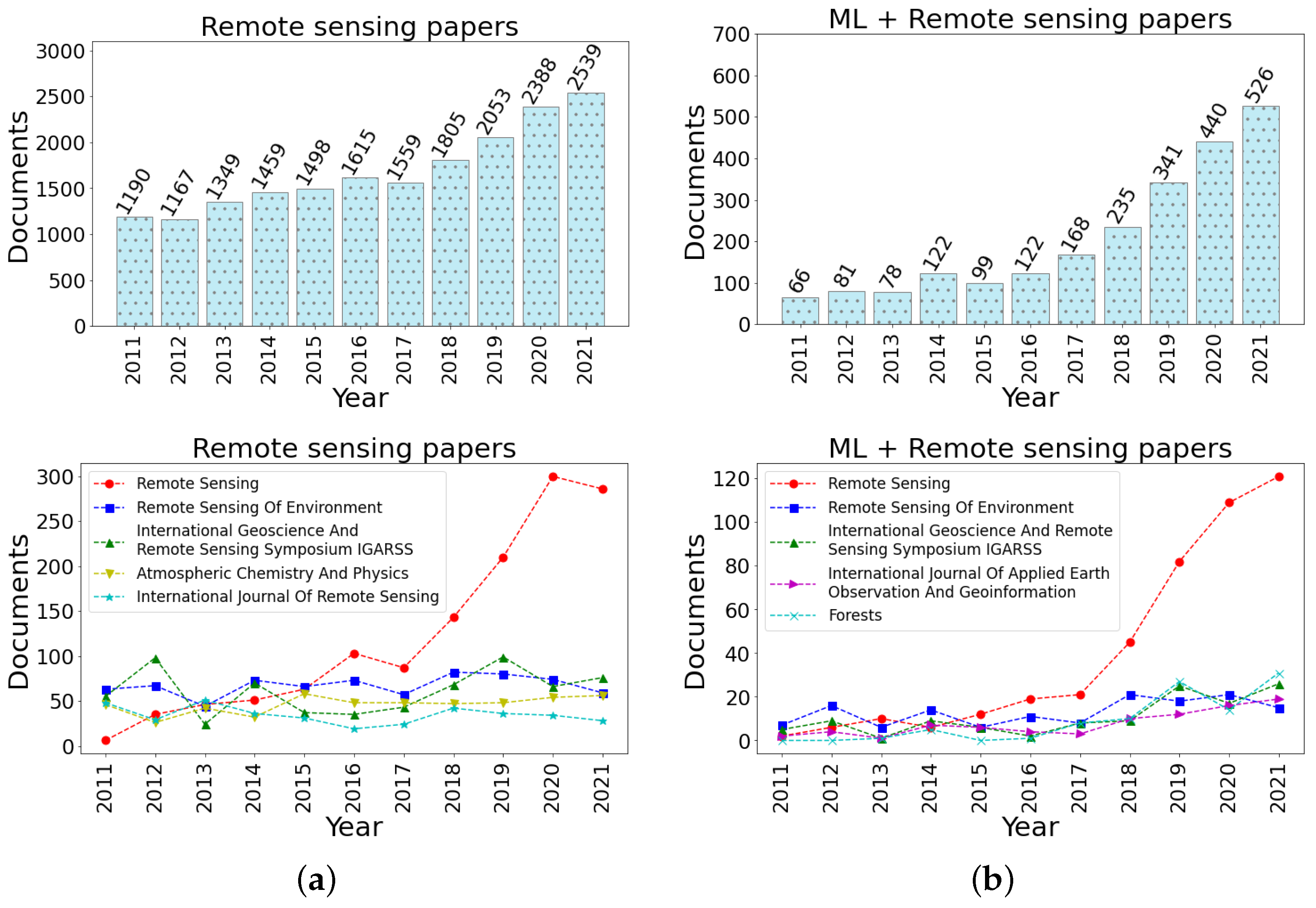
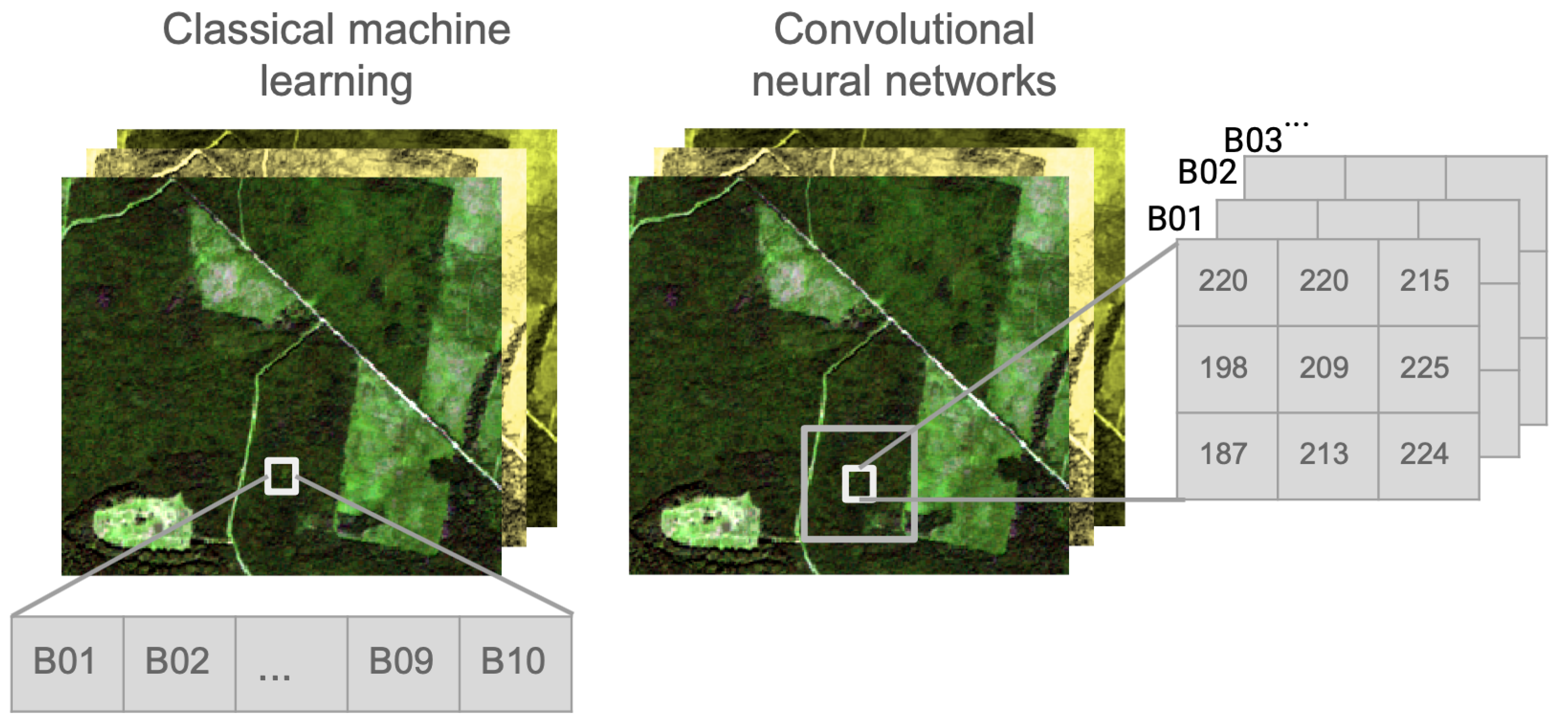
4.1. Classical Machine Learning Algorithms

To solve various tasks using RS data, one of the most effective and popular methods of classical machine learning is the random forest method (Random Forest, RF), which combines the approaches of an ensemble (a composition) of algorithms, namely, decision trees and the method of random subspaces. This method is widely applicable, for example, for solving problems of classification of forest-forming trees, as well as for solving regression problems, but it is not limited only to these tasks (described in Section 8). The ensemble is performed over multiple trees trained on different data subsamples, which helps one to avoid the overfitting issues occurring when only one decision tree is used. The resulting class or value prediction is made by averaging over all trees or choosing a class that is predicted by most of the trees. An important limitation of using a forest of trees compared to a standard decision tree is the interpretability of the results. Namely, a random forest of trees itself is much harder to interpret. The main parameters configured in the RF algorithm are as follows: the number of trees that determine the complexity of the algorithm; the number of features for splitting selection; the maximum depth of the trees responsible for the retraining and accuracy of the model; the criterion by which the homogeneity (entropy) of each leaf in the tree will be evaluated; the minimum number of objects at which splitting is performed, with a decrease in this parameter, the quality of training increases, but the training time also increases. One of the advantages of the RF algorithm is the speed of its learning process and ease of use, meaning that the algorithm is already implemented mostly with open-source programming languages and data analysis interfaces. For example, the Python Scikit-learn library [62] has an implementation that allows the user to quickly tune the hyperparameters and train and test the model.
Another effective method of classical machine learning capable of dealing with CV tasks for RS data analysis is the Support Vector Machine (SVM). This is a class of algorithms characterized by the use of kernels (including nonlinear ones) and the absence of local minima; they are aimed at solving both classification and regression problems. In the case of classification problems, the optimal hyperplane is determined, which provides the best separation of classes. SVM requires parameters to be tuned at the implementation, of which the main ones are the kernel type and its hyperparameters. One of the most popular kernel types is the Gaussian kernel (rbf), in which the C and γ parameters are configured for the misclassification penalty and the width of the kernel. It is necessary to vary the above parameters to obtain better accuracy and avoid over-fitting. Support Vector Regression (SVR) is based on the same approach as the SVM for the classification task, specifically, error minimization at determining the separating hyperplane for class extraction with a few slight differences.
The k-nearest neighbor (KNN) algorithm is a frequent choice for RS problems because of its simplicity and high interpretability [63]. It is a non-parametric supervised learning algorithm that commonly considers the Euclidean distance between an observed sample and its neighbors to make a prediction. The most similar data points are located closer to each other. Therefore, the class of a new data point can be estimated by voting the k most close points as the most frequently observed class. The number of neighbors (k) that participate in voting is defined empirically and depends on a particular task. The KNN algorithm can also be used for a regression problem. So, the output of the algorithms for the observed data point is the averaged target value for all k nearest neighbors.
The Gradient Boosting algorithm is also widely used in environmental studies both for regression and classification tasks. The boosting technique is an efficient ensemble approach when the model is built sequentially using weak learners [64]. Although gradient boosting can be based on different learners, the most common choice is decision trees. Each weak learner aims to minimize the error of the previous learner, being highly correlated with the negative gradient of the loss function of the previously assembled trees [65]. XGBoost (“Extreme Gradient Boosting”) algorithm is an adjustment of gradient boosting over trees that are based on the usage of a more powerful regularization technique to decrease over-fitting [66]. XGBoost supports parallelization within each tree, creating new branches independently, which makes the algorithm faster.
To adjust the quality of machine learning algorithms, one can apply the following approaches. For instance, the principal components analysis (PCA) is a dimensionality reduction method that creates a smaller dataset from a large amount of features preserving important information. This linear unsupervised statistical transformation was successfully applied to RS multispectral and hyperspectral data [67]. Another approach to reduce feature space is to use the RF algorithm for feature selection and then to train another machine learning algorithm with selected features. However, correlated features should be excluded as their importance might be underestimated. Another important option for model performance adjustment is optimal parameters selection. To optimize machine learning parameters, one can leverage various optimizations tools, such as Optuna [68], or scikit-optimize [69] (including Bayesian optimization).

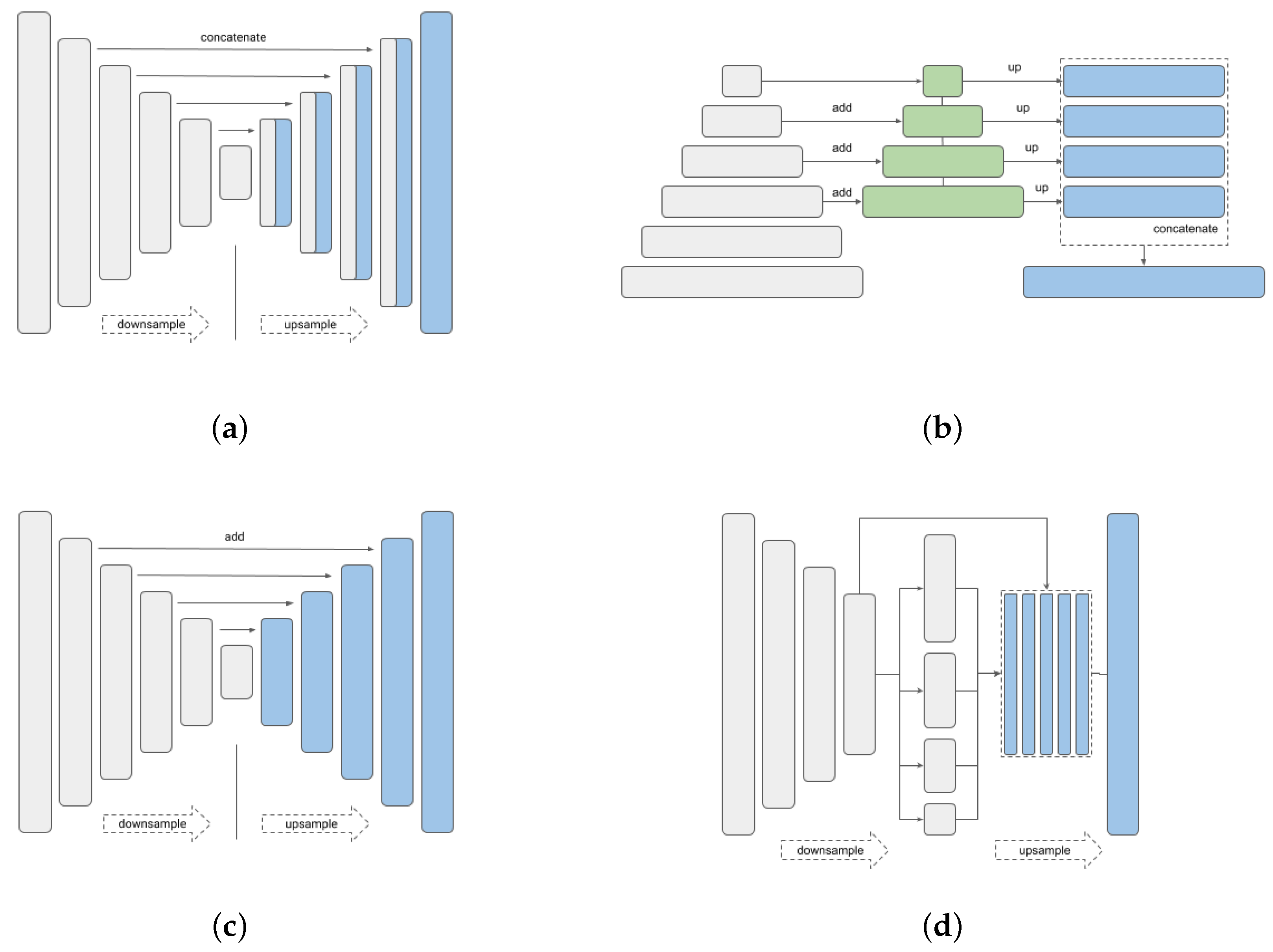
4.2. Deep Learning Algorithms

One of the main and frequently used architectures of CNNs for RS image processing, including the forest mask segmentation, is the U-Net architecture [70]. The schematic layout of various U-Net layers is shown in Figure 3a.
The architecture comprises two parts, forming a “U”-shape. The first part includes several convolution layers (parameters can be configured) responsible for feature selection. For a convolution operation, it is typical to use a 3-sized convolution kernel, followed by a nonlinear ReLU and Max-pooling layer for dimensionality reduction. The second part uses layers that convert a feature map from a compressed space into the initial dimension (deconvolution). Also, in the second part of the deconvolution process, there is an attachment of relevant maps of features obtained during the roll-up. As a result, the neural network’s output produces an image mask of the same size as the input image, where each pixel corresponds to a particular class. Training the neural network, namely, picking up values in the kernels, is effected by using the backpropagation method of the error. The neural network’s weight (trainable) parameters are updated iteratively based on calculated error. The error is computed using different loss functions (e.g., cross-entropy). The corresponding gradients for all layers and weights in the neural network are then updated.
L o s s = i = 1 N k = 1 C y i k log y ^ i k N ,
where N is the number of pixels, C is the number of target classes, y ^ is the probability predicted by the model that a pixel belongs to a particular target class, and y is the ground truth label of membership of a pixel in a class (0 or 1).
In addition, one can configure the importance of each class with weight functions so that the neural network can work with an unbalanced number of target classes.
Another efficient architecture for solving the problems of segmentation and mask selection is also worth mentioning—here we mean the Functional Pyramid Network (FPN) [72]. The schematic diagram (architecture) of FPN is shown in Figure 3b. This architecture has two parts, one from the bottom-up (convolution) and another from the top-down (deconvolution). One of the key features of this architecture is the simultaneous utilization of features of different resolutions and levels. The lower semantic weight (the lower generalizing ability) has high-resolution features, and the higher semantic weight has low resolution features. The lateral connections between the two paths make it possible to eliminate the problem of signal attenuation. As a result, it becomes possible to process the detailed information obtained at the bottom of the first pyramid and semantically significant features obtained at the top of the first pyramid.
Other neural network architectures relevant for RS tasks include FCN [73], DeepLab [74], LinkNet [75] (Figure 3c), PSPNet [76] (Figure 3d).
All mentioned architectures have the same prediction pipeline. Input data is passed from the first layer to the following layers. On each layer, the input signal is transformed depending on weights of artificial neurons and then fed to the activation function. Thus, non-linear data separation is enabled [77].
The neural network parameters as well as approach for its training takes a separate vital place in the development of effective algorithms for solving RS problems, in particular to characterize vegetation with the possibility of further conversion to carbon stock. The training parameters include the number of training epochs, the number of steps in each epoch, the size of the batch (sub-sample), and the size of the images that form the batch. The choice of these parameters affects the ultimate result of neural network predictions. Parameters monitoring and analysis during the training allow one to choose an optimal moment of training process termination and to avoid overfitting. Additionally, the convergence rate of the algorithm depends on the value of the step in learning (learning rate) and the choice of the optimizer. In many studies, it is proposed to use optimizers like SGD [78], Adam [79], and RMSProp [80]. The determination of the stopping moment for neural network training is often based on such indicators as the “plateau”. The “plateau” effect means that the validation sample’s accuracy does not increase during several epochs. Additionally, among the configurable parameters of the neural network, it is worth mentioning the importance of the CNN’s optimal size (depth). The depth choice depends on the problem to be solved and the amount of training data. Therefore, the number of layers and neurons is task-specific. For instance, for a small dataset, it is preferable to use a model with fewer learning parameters. However, if the dataset is large, common architectures with large amount of parameters are required. Such neural networks often do not fit a single GPU. To address this limitation, different approaches and strategies can be applied in order to train large neural networks effectively [81]. To deal with overfitting and to enhance model generalization, the dropout technique is usually implemented. It involves discarding some randomly selected nodes (both from input and hidden layers) during each training iteration. It reduces co-adaptation between neurons. During test time, dropout is not implemented, but weights are adjusted by the used training dropout ratio. However, some dropout modifications support their application during the test phase such as Monte Carlo dropout [82].

5. Evaluation Metrics

In this section, we describe the most commonly used metrics to evaluate ML and DL models. The input and output data are looked upon here as raster images (a more conventional representation for DL algorithms). However, the described metrics were applied to evaluate ML algorithms that work with individual spatial points and satellite features as tabular data.

5.1. Classification

To assess the per-pixel or region prediction quality of machine learning algorithms, the following inputs are used:
  • Per-pixel mask of the target classes, ground truth;
  • Per-pixel predicted mask with target classes.
Masks are in the raster format; the value of pixels belonging to the background is 0, and belonging to an object of the target class is 1 or more for a multiclass case. Therefore, when we have only two classes (target class and background), the mask has a Boolean representation. For instance, in the case of forest mask: areas covered by forest vegetation are marked with value 1, areas of other types have label 0. To calculate the prediction quality, True Positive ( T P ), False Positive ( F P ), True Negative ( T N ), and False Negative ( F N ) values are considered. True Positive is the number of correctly classified pixels of a given class; False Positive is the number of pixels classified as a given class while, in fact, being of another class; True Negative is the number of correctly classified pixels of another class; False Negative is the number of pixels of a given class, missed by the method. One can estimate the model quality based on the ratio between correctly classified objects and all objects representing the study area. This commonly used metric is Accuracy.
To evaluate the performance of neural networks for semantic segmentation or classical machine learning models, one can also apply an F1-score, which is widely used in RS tasks [83]. While the Accuracy metric is a good choice in the case of balanced classes, the F1-score is capable of effectively assessing the prediction quality for imbalanced classes. A high Accuracy score can be obtained for highly imbalanced data by assigning the majority class’s label to all observations.
Another popular metric for semantic segmentation tasks is IoU (intersect over union). F1-score and IoU are positively correlated metrics. However, F1-score is the harmonic mean, and IoU is closer to the minimum value between Precision and Recall.
The area under the curve (AUC) from the receiver operating characteristic (ROC) also helps to assess the quality of developed algorithms. True positive rate (TPR) and False positive rate (FPR) are estimated in order to build the ROC curve for different decision thresholds. We assume the model outputs certainty that the object belongs to the positive class. Therefore, these thresholds determine objects belonging to the positive class. AUC is the area for all possible decision thresholds for TPR and FPR combinations. It shows the model ability to range predictions correctly.

5.2. Regression

One can distinguish the following metrics from the most common metrics in regression tasks: mean absolute error (MAE), mean square error (MSE), root mean square error (RMSE), coefficient of determination ( R 2 ), mean absolute percentage error (MAPE), and mean bias error (MBE). Although MAE, MSE, RMSE, and MAPE aim to estimate how close the model prediction is to the actual values, they have differences. Depending on the task, they can be effectively combined for deeper model results analysis. Intuitive interpretation is indispensable for various practical forestry tasks. While MAE provides an error in the original unit of measure of actual target values, MAPE is commonly used to assess the error in percentages for more straightforward competitive analysis. Comparing MAPE and MBE with MAE, MSE, and RMSE, we can notice that only MAPE and MBE metrics take into account the position of the actual target and predicted values, i.e., a switching between these values leads to different results. MBE makes it possible to understand the model tendency for under- or overestimation of the target values as it can be both positive and negative. R 2 shows the relation between the total variance explained by the model and the total variance in actual target data.

6. Forest Mask Estimation on Remote Sensing Data

One of the initial steps in environmental studies based on RS data is the forest mask estimation. One can extract the required vegetation properties within such a mask, for instance, tree species, age, or canopy height. Another strongly related task to forest mask estimation is the deforestation problem, as it directly affects forest boundaries. The approaches to solve these two tasks are often quite similar. Selection of optimal data type and algorithm should always take into account the specifics of the problem to be solved. When ML methods are applied for these tasks one usually considers the semantic segmentation problem. According to the study requirements, different data sources can be used for this task. Therefore, both low, medium, and high spatial resolutions cover various cases with their advantages and disadvantages.

6.1. Use of Data of Different Spatial Resolution

6.1.1. Low Spatial Resolution

Low spatial resolution is recommended for regional and national assessments of forest cover characteristics. One of the popular sources of such data is imagery of the MODIS apparatus. Time series usage based on MODIS data with spatial resolution of 500 m in pixels has been successfully implemented in [84] to assess changes in forest cover in Brazil. For the same task of vegetation changes monitoring from MODIS images, the authors [85] demonstrated accurate results comparable to maps based on Landsat satellite data on a regional scale. The approach for rapid forest degradation assessment was proposed in [86]. Another commonly used data source for vegetation monitoring is ALOS PALSAR. In [87], it was proposed to use PALSAR radiometric data with a spatial resolution of 50 m in combination with MODIS multi-temporal data to obtain a forest cover map outside China.

6.1.2. Medium Spatial Resolution

Medium spatial resolution data are helpful for detailed forest mask segmentation. High revisiting time, public availability of data, and spatial resolution of up to 10 m per pixel make Sentinel-2 imagery a promising data source for many purposes such as forest mask estimation. In [88], Sentinel-2 imagery were used for assessing forest masks in Europe. Another source of multispectral data for forest plots is Landsat imagery. The effectiveness of Landsat and Sentinel imagery for forest degradation was demonstrated in [89]. The use of Sentinel-2 and Landsat data combination was recommended for tropical forest disturbance estimation [90]. In [91], the authors created a forest cover map for the territory of Germany and assessed the developed approach by comparing the generated map with national forest inventory data.
It was shown that Sentinel-2 data provide additional spectral information enriching aerial photography data for better predictions. Illegal logging drastically affects the state of the environment. Therefore, ERS is applied for operational monitoring with the aim at recognizing and preventing illegal logging. Medium spatial resolution satellite imagery is a suitable data source for logging detection because of the extensive coverage areas and rapid revisit time. Studies on illegal logging recognition using both multispectral and radar data were presented in [92,93]. In [94], the authors proposed a method for forest logging detection in Russia based on Landsat imagery. Time series are also considered in forest monitoring tasks on the medium spatial resolution satellite data. In [95], a time series based on Sentinel-2 imagery was used to assess the damage caused by windstorms in Italy. Forest degradation was also considered in [88]. For precise annual spatial distributions analysis, a time series was implemented in [96], where a robust mapping approach based on Sentinel-2 data was provided.
One can use open access maps and tools for vegetation area estimation and supplementary materials extraction such as cloud masks. Sentinel-2 provides a pixel classification map based on Level-1C data that includes the following classes: cloud, cloud shadows, vegetation, soils/deserts, water, snow, etc. The spatial resolution of the scene classification map is 20 m [97]. Pan-European High-Resolution Layers (HRL) is another useful tool for environmental studies, in particular, for forest cover estimation [98]. HRL is based on Sentinel-1 and Sentinel-2 satellite data. Tree cover density, dominant leaf type, and forest-type products are available for the reference year 2018 in 10 m spatial resolution.

6.1.3. High Spatial Resolution

High spatial resolution data are helpful when a more detailed forest mask is required, including separation individual trees, small tree groups, and small plots in a forest with meadows and tracks. In low or medium spatial resolution images, it is impossible to recognize with a high accuracy such details as an individual tree: an individual pixel covers an area exceeding 100 sq/m. To address this problem, one can use satellite images of high spatial resolution: WorldView, Spot, RapidEye, and Planet (see Table 1). Mapping eucalyptus trees were performed using high-resolution satellite data in [99], where WorldView-2 imagery usage provided a better accuracy than Spot-7 multispectral data. In [100], a method based on satellite data of very high spatial resolution for allocating individual crowns was proposed. A map with individual trees is helpful for detailed forest cover analysis. To assess forest degradation and forest cover change, WorldView data were used in [101]. In [102], an effective methodology was proposed for detecting illegal logging on small plots for the forests of Peru and Gabon. In [103], an approach using high-resolution data from RapidEye to monitor land cover changes (and, in particular, forest areas) was put forward. The deforestation problem was also considered using RapidEye data in [104]. The high spatial and temporal resolution of Planet images were utilized with LiDAR measurements to create the model for estimating the top-of-canopy height of tropical forests in Peru [105]. Images obtained from PlanetScope nanosatellite constellation were used to create a high resolution (1 m) map representing tree cover in African drylands [106], where a possibility to detect trees outside forests was shown.

6.1.4. Use of Data from Unmanned Aerial Vehicle

The very high spatial resolution provides a significantly better texture feature extraction than the medium spatial resolution. Therefore, unmanned aerial vehicle (UAV) data are often used for environmental remote sensing studies. Masking the forest with such data effectively used in assessing the state and environmental changes. To evaluate the effect of forest fires, UAV data has been successfully applied in [107]. The approach was based on using only RGB channels and has been tested for forest ecosystems in the Republic of Korea. In [108], a method for detecting and counting individual trees in images of different scales was proposed. To detect individual trees, UAV data have been successfully applied to mixed conifer forests [109]. Combining the data of various resolutions and spectral ranges, one can enrich a dataset with valuable features and achieve better prediction quality. In [110], the authors proposed using UAV data and photogrammetry as part of the overall research methodology and Sentinel-1 data to assess forest degradation. However, a severe drawback of UAV data usage for large-scale studies is the time and cost-consuming of its collecting.

6.2. Computer Vision Algorithms for Forest Mask Estimation. Specifics and Limitations of the Approach

Vegetation indices based on satellite spectral channels were suggested in many studies. For example, a methodology for assessing forest degradation based on the LAI index analysis using the MODIS data was given in [111] almost 40 years ago. Since then, vegetation indexes have been used in various studies as a simplest computer vision approach. In [112], the NDVI index (normalized vegetation index) was shown as being applicable to the forest degradation assessing task for the tropical forests of Malaysia. A significant drawback of such an approach was the requirement of a threshold choice for various satellite data, environment conditions, and seasons. Therefore, its reliability cannot be sufficient for precise analysis.
Classical machine learning methods are aimed at automatization of the forest mapping process. It requires less labeled data and computing capacity to train a model. Classical machine learning algorithms were compared in [113] for land cover classes separation, including forest areas. The authors reported better results for RF and SVM than for kNN. However, RF and SVM showed close results, with AUC values 0.81 and 0.79 . In [114], the SVM method, in combination with a submerged mangrove recognition index, was proposed to map mangrove forests with an overall accuracy of 94%. In [115], SVM with an RBF kernel function outperformed the RF algorithm in the CORINE land cover classification task. For forest area separation, an F1-score was found to be larger than 0.9 .
To solve the problem of forest mapping, one of the most common approaches is based on deep learning methods, namely convolutional neural networks (CNNs). The forest mask segmentation involves identification of the pixels belonging to a forest class. It is an example of a binary semantic segmentation task. For forest species classification (Section 7), the main difference is that a CNN predicts one of several classes for each image pixel. The major advantage of using a CNN over classical machine learning methods is that it takes into account spatial characteristics. When assessing a pixel label, CNN uses spectral information from the local area of the processed image. This provides a more accurate estimation of forest masks due to the forest spatial structure that the CNN also learns. The principal limitation of deep learning methods is the need for a large amount of labeled data to train the model. In addition, training neural networks usually requires a lot of time and computing resources.
One of the widespread CNN architectures for forest mask segmentation is the U-Net architecture. In [116], U-Net with Inception encoder was implemented to obtain a high-resolution (less than 1 m per pixel) detailed forest mask that also considers individual trees outside the forest. Due to spatial texture features, the CNN-based approach provides robust results for various territories using just RGB images. The authors also noticed that a comparison between U-Net and FPN models gives better outcomes for the U-Net model (F1-score of 0.929). U-Net was also implemented for very high spatial resolution in [117]. For the medium spatial resolution of Sentinel-2 data (10 m per pixel), a modified U-Net with attention mechanism shows high performance [118]. The authors declared the advantage of U-Net architecture versus ResNet and FCN for experiments with different locations using RGB bands and RGB plus NIR. An example of application and comparison of U-Net, DeepLabv3+, FPN, PSPNet, and LinkNet architectures in Brazil’s Eucalyptus Forest mapping task on medium spatial resolution data (Sentinel-2) was shown in [119]. The best result with IoU of 76.57 using DeepLabv3+ with the Efficient-net-b7 backbone was achieved.
To deal with limited labeled data and adjust CNN model performance, one can apply transfer learning techniques. In transfer learning, the pre-trained model is adopted for new tasks and data specificity. In [120], transfer learning was used for forest mapping with subsequent fine-tuning of the model over the target forest domain. The proposed approach enables one to extract features from unlabeled data and using them for progressive unsupervised CNN training.

7. Forest-Forming Species Classification on Remote Sensing Data

After estimation the tree cover area as a forest mask, the next important step in forest taxation is determining tree species. This is especially relevant for large territories and locations, which are challenging to access [17]. In terms of CV, achieving the goal of tree type classification is also based on the solution of the image semantic segmentation task. Although the determination of tree species includes mostly more than two classes, the approach remains the same. Each image pixel needs to be labeled according to the class based on the test data for the algorithm training.
The most commonly used metric for estimation of the quality of tree species prediction from image data is the F1-score. Just as was described earlier in the case of forest mask estimation, the evaluation of the F1-score is carried out for each class individually. The closer the resulting value is to 1, the more similar are the prediction and reference labels.

7.1. Use of Data of Different Spatial Resolution

The use of the data of different resolutions is determined by the problem that needs to be solved via the knowledge of the tree species composition across the area of interest. In general, at different spatial resolutions, estimates of tree species composition may be required for purposes of mapping large and difficult-to-access areas for biomass and carbon estimation [121], to access succession trends on disturbed regions for a better understanding of carbon accumulation patterns [122], to link climate effects with forest management activities [123], for tree mortality monitoring and capturing of its patterns at different scales [50,124], and natural and urban ecosystem assessment [125].

7.1.1. Low Spatial Resolution

Similarly to forest mask determination from low spatial resolution data, Terra MODIS satellite imagery is a common choice of satellite data for forest species classification. An approach to determining the dominant species using the MODIS sensor data with calculation of vegetation indices from multi-temporal images was proposed in [126]. Additionally, the use of low spatial resolution data for solving a similar problem was proposed in [127], and [128]. However, it was shown that coarse-scale satellite data might not capture many of the target processes, e.g., degradation development [89], so recent low-resolution data are often used for obtaining more general, aggregating characteristics. Such information can be considered as a distribution of a set of unique surface characteristics reflecting environmental conditions similarly, and mostly represented by land cover type classification [129], temporal dynamics of the distribution of derivatives such as vegetation indices [130], or plant functional types [131]. Combination of low spatial resolution data with more detailed imagery, e.g., MODIS data together with Landsat satellite data, as was shown in [132], is a current trend.

7.1.2. Medium Spatial Resolution

A more detailed forest species determination can be achieved using the data of medium spatial resolution, for example, obtained from Landsat and Sentinel missions.
The authors in [133] suggested using Sentinel-2 data to identify tree species in central Europe. In [134], an approach based on a combination of ML algorithms was also presented for classification of tree species in German forests. Another approach based on an application of linear discriminant analysis to medium spatial resolution images was proposed in [135]. Sentinel-2 data was also proposed for solving the problem of identification of forest species based on a series of images for different dates [49]. In [49], the authors succeeded to increase overall accuracy from 72.9% to 85.7% by using of the multi-temporal analysis. Radar data can adjust multispectral-based predictions, it was shown for Sentinel-1 and -2 data in the task of forest and plantation mapping and stand ages prediction [136]. For better understanding of forest properties and patterns, it is possible to use hyperspectral RS data. It contains a wide continuous range of electromagnetic spectrum, while in multispectral sensing, discrete wavelength regions are considered. As an example, the Hyperion instrument on board the Earth Observing-1 (EO-1) spacecraft with 30 m spatial resolution provides 220 spectral bands for diverse environmental studies. In [137], Hyperion data were used to classify mangrove species and to analyze their changes over a period of time. Forest species distribution was assessed in [138]. Forest properties can be also effectively discriminated using the new hyperspectral Precursore IperSpettrale della Missione Applicativa (PRISMA) sensor, launched in 2019 and providing spatial resolution of 30 m [139]. These hyperspectral data are also accompanied by 5 m panchromatic band. PRISMA data usage showed high results compared to Sentinel-2 for forest categories classification [140]. Although it is a promising RS data source, there are at present a few studies considering its usage for vegetation analysis compared to more conventional data such as Sentinel-1 and -2, Landsat-7, etc. [141].

7.1.3. High Spatial Resolution

High spatial resolution data allow one to operate not only with the spectral description of the object under study, but also with its textural and spatial characteristics. For example, the WorldView-2 panchromatic channel with a resolution of about 0.5 m (depending on the geographic latitude of the survey) can be effectively used to determine the shape of a tree crown. It in turn increases the likelihood of correct classification of tree species. In addition to more detailed information from satellites providing high spatial resolution images, the possibility of using time series, as in the case of data of lower spatial resolution, is also an advantage of the approach. For example, the authors in [142] successfully implemented multi-temporal WorldView images for forest hardwoods classification. In [143], tree species were classified for tropical forests based on 16 high-resolution WorldView-3 bands. One of the advantages of the WorldView-3 mission is the new SWIR sensing capabilities. Mangrove species classification study was conducted for WorldView-2 data in [144], where the overall accuracy 95.89% was achieved. Although WorldView-2 and UAV data provided high results individually, their combination allows one to extract the most relevant features for classification.

7.1.4. Use of Data from Unmanned Aerial Vehicle

Hyperspectral and multispectral airborne images are known as a significant source of data for determining forest inventory characteristics [145,146,147]. The use of data-rich in both spectral and spatial features can handle the recognition of multiple tree species even in the case of complex terrain. Such approach provides an efficient classification on a small data set in the presence of many classes. Additionally, it is often proposed to use a combination of these data with LiDAR measurements [148]. An example of multi-copter UAVs with spatial resolution less than 2 cm was described in [149]. The study area covered 51 ha in Germany, which was sufficient for the representative analysis.

7.2. Computer Vision Algorithms for Classifying Forest-Forming Species Types. Specifics and Limitations of the Approach

RF algorithm has demonstrated the ability to classify forest species, for example, when obtaining a forest map in Wuhan, China [150]. The RF algorithm can be used as part of a hierarchical tree type classification methodology. In the first stage, it is possible to provide classification according to vegetative indices such as NDVI and RBI (Ratio Blue Index), then classify forest areas and tree types using RF. SVM is broadly used for forest type classification in [146,151]. A combination of LiDAR and hyperspectral data was used in [152], where SVM outperformed other classical machine learning methods with respect to the OA metric for species classification. However, in [144], better results were achieved for RF than for SVM algorithm, with the best OA of 95.89 % for species classification.
Both classical machine learning and deep learning algorithms can handle a single image and a sequence of images covering the same region. For instance, in [153], all available images were combined to train an RF model and to predict four forest species with OA of 88.2 %. One of the limitations of using a series of multispectral satellite images is the occurrence of cloud-contaminated images, which can corrupt predictions.
Similarly to solving forest area segmentation tasks, deep learning methods (CNNs, specifically) can be used for determination of forest species types. The main difference from the forest segmentation task is that several classes of pixels are predicted, corresponding to classes of tree species. We provide more details about the adjustable parameters of neural networks and their features in Section 4. An essential step in classification of tree species is determining the crown shape, for which high spatial resolution images are needed. Thus, when working with high spatial resolution images, a CNN makes it possible to create an optimal feature space that characterizes various forms of crowns, leading to a more accurate classification. For instance, in [154], the developed CNN was shown as being capable of classifying tree species based on biological structures such as foliage shapes and branching patterns. It is essential when just RGB bands are used, and different forest species may have the same colors. Three of seven considered classes were classified with OA over 90%. Due to very high spatial resolution of UAV, approach was capable of individual tree mapping. The U-Net architecture is also used to perform a hierarchical classification of dominant species [155], where deciduous and coniferous forests are classified separately. Next, tree types were determined within each class (conifer and deciduous). Such a hierarchical approach helps to address the class imbalance problem by splitting classes into smaller subsets and simplifying the semantic segmentation problem for a CNN. The hierarchical approach leads to the result improvement from F1-score of 0.69 to 0.83 compared with “one versus all” classification. The effectiveness of the U-Net, U-Net++, and DeepLab architectures for the forest dominant species estimation in the boreal region was also demonstrated in [156]. These three architectures showed comparable results. In [147], U-Net architecture was modified for forest species classification __combined U-Net with the feature __ extraction network ResNet. The OA was equal to 87%, which is higher than the initial model results. Another architecture improvement is described in [157], where a class imbalance problem was addressed. The approach involves jigsaw resampling strategy to create a balanced training dataset. New training samples with the size of 128 × 128 pixels are combined from smaller patches with the of 32 × 32 pixels, where each small patch covers a single tree species. Proposed approach improved the baseline from 66% to 80% (quality is measured as the proportion of correctly classified pixels to total pixels). The high-resolution data provide significant features for a CNN model and facilitate its accurate predictions when a sufficient amount of data (over 51 ha with spatial resolution less than 2 cm) are available [149]. Different tile sizes and spatial resolutions were examined. It was shown, that large tile size is preferable in case of a sufficient amount of training data. The best model with optimal tile size and spatial resolution achieved an OA of 89% and mean F1-score of 73%. It is also possible to use approaches that combine data from several sources to provide better accuracy. RS images can be supplemented with phenological parameters and forest stand structure data. Although such features can be extracted from forest inventory data, another approach is to train a model to predict it. For instance, in [158], the canopy height was estimated using a CNN model. Next, these predictions are used to supply multispectral data in a forest-type classification task.

8. Forest Resources Estimation on Remote Sensing Data

In this section, we discuss the following forest variables: aboveground biomass, standing volume, and growing stock volume. The definition of aboveground biomass (AGB) is the aboveground standing dry mass of live or dead matter from tree or shrub (woody) life forms [159]. We refer to growing stock volume (GSV) as ”volume of living and standing stems over a specified land area that includes the stem volumes from stump height to the stem top and the bark but excludes the branches” [18]. The standing volume is defined as “the volume of standing trees, living or dead, above stump measured over bark to the top. It includes all trees regardless of diameter, tops of stems, large branches and dead trees lying on the ground which can still be used for fibre or fuel” [160]. These variables have a strong relationship and are considered as quantity measurements of forest and its derivatives. An assessment of forest resources helps to effectively determine the forest carbon stock. Therefore, such forest attributes estimation using RS data is an important area of machine learning methods application.
The problem of aboveground biomass, timber volume, and growing stock estimation is often solved as a regression problem in the following way. The regression task for RS data is a machine learning task, where the model is trained to assign some real value to each pixel of the resulting digital map of the target territory. A machine learning model uses a training set to determine the relationship between the feature description of objects and the target value. Thus, just as in the semantic segmentation problem, the ground truth image with the reference markup is used. During the training procedure, a model reduces the difference between the prediction and the reference values according to the chosen quality metric.

8.1. Use of Data of Different Spatial Resolution

8.1.1. Low Spatial Resolution

To obtain timber volume estimation on a large scale, it is often proposed to use MODIS sensor data. Approaches for determination of forest biomass are presented in [161,162,163]. The data effectiveness was verified for regional changes monitoring and supplemented forest inventory data for ecological assessment. Despite the possibility of a large spatial coverage supported by this approach, for some practical problems, more detailed maps are required. Therefore, one can consider higher spatial resolution data.

8.1.2. Medium Spatial Resolution

When it is necessary to estimate timber volume over a large area with greater details, a common choice of RS data is medium spatial resolution. For example, this type of data can be received from Sentinel and Landsat satellites. The potential of using Sentinel-2 data to determine growing stock volume for the territory of Italy was demonstrated in [164], where the prediction quality based on Sentinel-2 data was shown to be better than that for Landsat images in 37.5% of cases and for RapidEye images in 62.5% of cases, even though the resolution of the RapidEye satellite is significantly higher than that of Sentinel-2. In [165], Sentinel-2 data was shown as being capable of determining growing stock volume in Russia. Additionally, Sentinel images were used in [166] to map the timber volume in the coniferous forests of Norway. The relevance of using these data was also confirmed in other works on determining the biomass and stock volume in various territories [167,168].
Another useful instrument for environmental analysis that deserves additional consideration is GEDI. It is the first spaceborne lidar that was developed exactly for environmental monitoring purpose. It has a medium spatial of 25 m. One of its goal is to provide a better understanding of the aboveground carbon balance of the tropical and temperate forests [169]. It can accompany other RS data for enhanced biomass mapping and help to estimate aboveground carbon change.

8.1.3. High Spatial Resolution

Commonly, high spatial resolution data is used when it is required to estimate timber volume down to a single tree. In the actual studies on this topic, it is recommended to use WorldView satellite images with a resolution of about 2 m for a spectral range of channels from 396 nm to 1043 nm and sub-meter resolution for the panchromatic channel. An example of using WorldView-2 stereo images was demonstrated in [170], where high-resolution data and LiDAR measurements were compared in the problem of assessing the timber stock for the forest area in Germany. In [171], panchromatic WorldView-2 stereo-imagery is considered together with a digital elevation model derived from airborne laser scanning. Using WorldView imagery for different geographic regions was also confirmed by a study of Turkish forests in [172]. Forest standing biomass was estimated and used to assess forest productivity in [173] based on WorldView-2 data. The authors evaluated the importance of different bands and vegetation indices and highlighted the Red-edge band significance. Spot-5 is another source of high-resolution data for aboveground biomass estimation [174].

8.1.4. Use of Data from Unmanned Aerial Vehicle

UAV data are selected for land cover surveys in cases where very detailed timber volume estimation is required. The use of UAVs makes it possible to analyze the characteristics of an individual tree by constructing a more informative feature description of the vegetation cover with a resolution of up to several centimeters per pixel. The approach to determining the timber volume based on UAV images and photogrammetry was tested with success in [175]. One well-established approach to forest growing stock volume estimation is based on using satellite imagery in combination with UAV data [176]. This approach’s advantage is combining the spectral features obtained from the satellite with highly detailed textural features. In [177], an approach to replace ground-based measurements for growing stock volume estimation with UAV data was used with good results. At the same time, ground-based measurement data were used in this research only to assess the quality of algorithm predictions. In [178], data with a spatial resolution of less than 10 cm per pixel were used to determine the stand volume. In [179], images with the same spatial resolution were used to estimate forest biomass. It was presented the effective use of UAV data for tree stem assessment in [180,181,182]. Not only images can be used for forest analysis. Point cloud obtained from UAV can also be considered in voxel-based representation for further computer vision algorithms application, as shown in [180]. In [181], dense points cloud derived from multicopter is used to extract significant characteristics for stem volume prediction using machine learning algorithms. For instance, they estimated the height of the forested area by subtracting the digital terrain model (DTM) from the digital surface model (DSM). DTM was obtained from terrestrial laser scanning, while an unmanned aerial system was utilized to get DSM.
Although UAV provides very-high resolution data, one of the significant limitations of UAV-based approaches compared to satellite data is the relative laboriousness of obtaining such data on extensive areas.

8.2. Computer Vision Algorithms for the Task of Forest Resources Estimation. Specifics and Limitations of the Approach

In many studies, it was demonstrated the effectiveness of the linear regression algorithm in the problem of timber stock evaluation. The advantage of this approach is the ease of implementation and use. In addition, an important characteristic is the interpretability of the results. The work [183] proposed to use linear regression to estimate the diameter of tree crowns from UAV data. An approach based on multiple linear regression was presented in [184]. The described method makes it possible to determine the stock of plantations on pine plots using Sentinel-2 images and aerial photography data. Different RS data sources and spatial resolution make it important to preserve the same data georeference. Ground Control Points (GCPs) were used to calculate UAV’s camera orientation and set a correct georeferencing. Prediction of growing stock using a linear regression algorithm based on Landsat-7 images is demonstrated in [185]. Both vegetation indices and linear regression were implemented in [174].
It is also proposed to use the Random forest regression (RFR) algorithm for timber stock estimation. The approach based on ultra-high spatial resolution data is described in [181], where various RS measurements were considered. The methodology includes a stratified random sampling of training examples and algorithm parameter optimization. The parameters used in the RFR algorithm are described in more detail in Section 4. Besides the problem of determining the stock of wood, the problem of estimating the stock of carbon can be also directly solved using RS data and RFR algorithm. This approach was tested for mangrove forests in [186]. In this research, various forest cover characteristics were used to assess the stock: tree species, height, and textural features. Vegetation indices based on UAV spectral data were also used to form the feature space. The most significant features were selected based on the Boruta algorithm [187]. It is also important for UAV-derived multispectral data to conduct a reflectance calibration of cameras to support accurate temporal analyses because digital numbers are affected by the atmospheric and illumination conditions and cannot be considered as quantitative values [188].
SVR is another relevant approach for stem volume estimation [181]. An approach for biomass estimation using the SVR algorithm with a radial basis function (RBF) kernel was proposed in [189]. As it was shown earlier in Section 4, it is important to find the optimal parameters of the algorithm, which can have a significant effect on the final accuracy. In [189], the kernel parameters were selected using the grid search method. The feature space was formed based on various RS data sources: Sentinel-1 radar data, Sentinel-2 multispectral images with 10 vegetation indices obtained on their basis, and UAV photogrammetry data. The use of the SVR algorithm for biomass estimation was also proposed and shown to be effective in other studies [190,191].
Above-ground biomass estimation with the use of CNNs was examined in [192]. The prediction results, as measured by R2, were found to be equal to 0.943 . The aboveground carbon density of forests can be estimated directly using RS data and a CNN model, as was demonstrated in [193], where a CNN model was shown to perform better than classical machine learning algorithms. In [194], a CNN-based approach yields RMSE of 20.3 % for the volume of growing stock estimation using airborne laser scanning. Although CNN is highly promising for such studies, no strong difference between the k-NN and CNN performance was observed. It was suggested that additional data should be utilized to reveal the full potential of CNN models.
For more accurate growing stock volume estimation on the limited dataset size, a deep neural network with transfer learning was implemented in [195]; this approach allowed the authors to minimize the amount of ground-based measurements over different areas in Finland.

9. Discussion

Based on the current trends in development of satellite imagery and data processing algorithms, we expect the following trends in this domain. First of all, there is more availability of high quality reference data for artificial intelligence algorithms and build-in services for data processing that are provided by the space companies. Advanced systems and cloud computing platforms will be easy to use even for inexperienced users. Satellite constellations will have better revisit time and coverage, allowing near real time observation of ground cover. Additionally, high resolution multispectral imagery will be wider applicable, giving important information about investigated objects including forests. Developments of special augmentation techniques and a few short learning algorithms will allow us to detect and make more precise quantitative assessment of forest variables and forest disturbing events. In this section, we provide more details about current limitations and future works.

9.1. Forest Carbon Disturbing Events

Improved forest management in terms of carbon offsetting is based on carbon sequestration from the atmosphere. Precisely, it means the storage on a long-time basis of more carbon compared to the regional baseline in the ecosystem considering land-use practices, maintaining existing forests, and increasing total forest coverage, while decreasing mortality [196,197]. On both large scales and in the case of small forest landowners and land rent, this means enhancing carbon pools, thereby reducing emissions caused by different processes of GHG into the atmosphere. At the same time, the above-ground biomass of living trees is considered the most dynamic carbon pool affected by the plethora of factors of distinct nature [198]. Such forest carbon disturbing factors include the development of areas inundated with water and changes related to them and the soil hydrologic cycle in general [199], the occurrence of deadwood due to the influence of biotic and abiotic events [200], wildfires and harvesting [53,201]. Detection, attribution, and monitoring of such occurrences can be covered using RS techniques. In this way, CV approaches should also be considered for fully and semi-automated solutions development, while a wide range of stakeholders can use such solutions to plan and implement climate change mitigation strategies based on nature preservation actions.
Studying flooded areas in terms of CV is accompanied by multi-challenging tasks. Among the major ones, we mention the following tasks: detection of flooded territories themselves and changes catching [202]; distinction between different types and classes of flooded lands [203]; estimation of biomass and potential to CO2 sequestration [204]; fusion of data of different domains to catch emission patterns and enhance accounting [205,206]. Such research is based on the solution of segmentation and classification tasks. A broad range of tools for these tasks involves conventional unsupervised and supervised ML algorithms such as RF, SVM, XGBoost, random walker segmentation, different types of neural networks (mostly deep CNNs) variations of edge detection, and others. In [207], the performance of CNN, AlexNet was compared with classic RF to distinct and map different wetland types, including bog, fen, marsh, swamp, and also shallow water, and deep water along with urban areas and upland. In this study, RapidEye multispectral imagery and a small number of input features were used. CNN was shown to overperform RF, catching both the dominant wetland classes and detailed spatial distribution of all studied land cover classes, which showed an overall accuracy and Kappa coefficient of 94.82% and 0.93, respectively. In [208], RF, as declared a computationally efficient and easily adjustable algorithm, was applied to multi-year summer composites of Sentinel-1 and Sentinel-2 images. Wetland spatial distribution was mapped, considering wetland classes across Canada, covering an area of approximately one billion hectares. The model accuracy varied from 74% to 84% in different territories.
Similarly to wetland research, studying and monitoring wildfire events are comprehensive and consist of the following main aspects: early fire and smoke detection; estimation of fire severity and spread; fire behavior analysis and prediction; and detection and estimation of post-fire territories. Forest fires are extremely hazardous to both natural ecosystems and humans, destroying habitat areas, negatively affecting agriculture, and accompanying significant emissions of retained carbon. Thus, related monitoring and detection technologies are rapidly developing, so, for instance, several satellites with low spatial resolution but short revisiting time already have fire detection sensors onboard [209,210]. The combination of UAV-based RS with CV techniques, based explicitly on CNN, including previously discussed architectures such as U-Net, DeepLab, and other deep learning architectures such as, e.g., GAN and LSTM, is an effective tool for wildfire monitoring. It is extremely useful for firefighting actions and capable of catching early fires in reduced time and more safely compared with ground inspections [210]. Such solutions can provide real-time monitoring, but require powerful hardware. An original Burnt-Net inspired by U-Net architecture was used for the development of an end-to-end solution for post-fire tracking and management. It was utilized to map burned areas on Sentinel-2 images across different countries, including Cyprus, Turkey, Greece, France, Portugal, and Spain, showing high robustness and mean accuracy of more than 97% by overall accuracy [211]. In [212], Maximum Likelihood, SVMs classifiers, and two multi-index methods were compared for mapping burnt area. Burn severity was also assessed using SVMs and one hidden-layer NN on Sentinel 1,2 images on the study location in Portugal. According to the results obtained, SVMs showed the highest accuracy for both burnt area mapping and burn severity levels estimation, with achieved an overall accuracy of 94.8% and 77.9%, respectively.
Deadwood represents essential carbon stock while simultaneously a significant contributor to carbon dioxide emission and one of the major forest biodiversity loci [213]. The development of deadwood can be a consequence of the natural course of things or triggered by biotic and abiotic factors such as pest or pathogen outbreaks, changes in hydrologic regime due to climatic shifts, and windstorms [214,215]. Numerous studies are dedicated to find a difference between target object (deadwood occurred due to a specific reason) and other nontarget objects, or, for example, between damaged trees at different stages of factor influence, existing together and displaying similar spectral signatures [216,217]. For instance, in [218], it is recommended to apply a Neural Net with standard backpropagation and SVM among other supervised approaches for the deadwood detection in the case of Chilean Central-Patagonian Forests using high-resolution multi-spectral data (RGB+NIR) with the best algorithm performance of 98%. In [219], an approach based on CNNs fusion of Lidar and multispectral data was applied for 3D tree type classification along with dead trees, showing an overall accuracy of more than 90% for all classes. At the same time, it was noted that the use of lidar-based data slightly increased the overall accuracy. The proposed comprehensive solution facilitates fast model convergence, as was pointed out even for datasets with a limited number of samples due to the applied transfer learning technique.

9.2. Data and Labeling Limitations

Training an accurate and robust computer vision model requires representative data that cover many possible scenes and are obtained under different illumination conditions. Training models with many parameters on non-representative dataset with low number of samples could lead to model overfitting. The use of models with small parameters that could be trained on a small member of parameters does not allow one to obtain acceptable accuracy and generalization. For a recent comprehensive analysis of overfitting and underfitting reasons in machine learning applications for different domains, see [220].
Computer vision models for processing RS data are not an exception. A large amount of well-annotated spatial data is required to train algorithms [221]. Moreover, there are many additional issues that appear due to the complexity of the data collection procedure. It is difficult and time-consuming to collect and directly label the amount of representative RS data. The principal impediments are weather conditions (clouds) and satellite (sensor) revisit time [222,223]. Thus, expanding the dataset with additional useful and reasonable data is vital. One way to solve this problem is to generate image samples from the obtained data. The most common approach for generating new image samples is augmentation. Several typical augmentation approaches are widely used in different domains, starting from classical augmentations, which include geometrical, and color augmentations, and finishing with application of ML techniques for augmentation [224]. Nevertheless, new approaches are in high demand and still appearing [225]. However, there are many restrictions in applying augmentation techniques for RS data because images may have a complex structure [226]. For example, the relative locations of objects should be meaningful after the creation of the new image sample. That is why it is important to carefully tune the parameters of augmentation when applying even standard augmentations carefully. However, there are some new advanced augmentation approaches that take into account the specifics of RS domain. For example, in [227], an approach was put forward capable of processing individual objects in the obtained image (RS data) and creating a new image sample that includes a meaningful composition of the target objects. A different augmentation approach proposed in [228] uses the multispectral specifics of RS data. The main idea of the proposed approach is the generation of a new image sample by mixing spectral bands from the satellite images collected for the same area but at different times.
The other limitation in the use of RS data in computer vision models is the involved labeling procedure. Only an expert can create a precise manual markup with vegetation characteristics based on these images (distinguish forest species, age, etc.). Ground-based measurements also have particular limitations. For instance, forest inventory data can be out of date. It also has some specificity in its organization. Information is often available for individual stands that are not necessarily homogeneous. Therefore, the dominant forest species (and other characteristics) are estimated in various tasks. It leads to some mismatches in training data. As a result, CV methods in environmental studies aim to work with invalid markup in particular cases. It is essential to develop a methodology for automatic improvement of RS data labeling. One popular approach is the weakly supervised learning, which is considered a fundamental problem in machine learning [229]. For land cover mapping and, in particular, forest areas, weakly supervised segmentation was suggested in [230]. In [231], the problem of weakly supervised pixel-level mapping to predict tree species was addressed. Weakly supervised classification for forest species estimation was proposed in [156] extract more homogeneous areas within individual stands.
To address spatial and temporal limitations in concrete environmental and forestry tasks, a combination of Sentinel-2 and Sentinel-3 data can be used. In [232], it was applied for evapotranspiration estimation. Although, there is a high importance of thermal features obtained from Sentinel-3, their spatial resolution requires adjustment. Sharpened high-resolution thermal data usage was suggested as a promising approach for environmental studies.

9.3. Visual Transformers as State-of-the-Art CV Algorithms Relevant for Forest Taxation Problem

Visual transformer-based approaches, which have appeared relatively recently, have also been used for dealing with problems of classification on environmental RS data [233,234] and change detection [235]. These approaches can also be applied to forest characteristics assessment. Transformer approaches are currently the most advanced models. These approaches use multi-purpose attention mechanisms as the main building block for obtaining long-term contextual information and links between pixels in images rather than standard layers. In the first step, the analyzed images are divided into groups and then transformed into a sequence by constructing a new feature space. The resulting sequence is then fed to several attention layers to form the final new presentation. The first sequence of tokens is used in the classification layer at the classification stage. The detailed description of self-attention mechanisms and pretraining procedures in visual transformers are described in [236]. One of the essential advantages of transformers is the possibility of compressing the network and removing half of the layers while remaining a sufficiently accurate classification [233]. Experimental results from various environmental RS data image datasets [233,234,235] demonstrate the potency of transformers compared to other methods.

10. Conclusions

The present survey discusses the key aspects of forestry analysis based on RS data and computer vision techniques. The study was focused on the particular forestry problems such as estimation of forested areas, tree species classification, and forest resources evaluation. These tasks are highly valuable for meaningful environmental analysis involving carbon stock monitoring and global climate changes. In these tasks, we aimed to emphasize both algorithms and data importance. Although various satellite missions and UAV-based approaches support effective solutions, the main current limitation is a lack of high-quality reference data for artificial intelligence algorithms. Additionally, it has been shown that data source and algorithm choice strongly depend on the objective of the study, as temporal/spatial resolution and cost may vary drastically. For large-scale analysis, satellite-based approaches are more preferable because of broader coverage, while for more detailed measurements, UAV-based approaches allow one to achieve the required results. Various RS data combination and advanced computer vision techniques such as few-shot learning, transfer learning, weakly supervised learning, visual transformers, augmentations techniques show promising perspectives for further environmental studies. At the same time, physical nature of the observed environmental objects should be taken into account both during the data acquisition, processing for computer vision algorithms, or vegetation indices implementation.

Author Contributions

Conceptualization, S.I., D.S. and I.O.; methodology, S.I., D.S., A.E. and E.B.; investigation, S.I., D.S., P.T. and V.I.; writing—all authors; supervision, I.O.; project administration, E.B. and A.E.; funding acquisition, E.B. All authors have read and agreed to the published version of the manuscript.

Funding

This work was supported by Ministry of Science and Higher Education grant No. 075-10-2021-068.

Conflicts of Interest

The authors declare no conflict of interest.

Abbreviations

The following abbreviations are used in this manuscript:
ARVIAtmospherically Resistant Vegetation Index
BAIBurned Area Index
CNNConvolutional neural network
CVComputer vision
DLDeep learning
EVIEnhanced Vegetation Index
FPNFunctional pyramid network
GHGGreenhouse gas
kNNk Nearest Neighbor
NBRNormalised Burn Ratio
NBRT Normalised Burn Ratio Thermal
NDMINormalized Difference Moisture Index
NDVINormalised Difference Vegetation Index
NDWINormalized Difference Water Index
NIRNear-infrared
OAOverall accuracy
RFRandom forest
RSRemote sensing
LDLinear dichroism
LSWILand Surface Water Index
MLMachine learning
SAVISoil Adjusted Vegetation Index
SVMSupport vector machines
SWIRShort-wave infrared reflectance
VCIVegetation Condition Index
UAVUnmanned aerial vehicle

References

  1. Peters, G.P. Beyond carbon budgets. Nat. Geosci. 2018, 11, 378–380. [Google Scholar] [CrossRef]
  2. Treat, C.C.; Marushchak, M.E.; Voigt, C.; Zhang, Y.; Tan, Z.; Zhuang, Q.; Virtanen, T.A.; Räsänen, A.; Biasi, C.; Hugelius, G.; et al. Tundra landscape heterogeneity, not interannual variability, controls the decadal regional carbon balance in the Western Russian Arctic. Glob. Change Biol. 2018, 24, 5188–5204. [Google Scholar] [CrossRef] [PubMed] [Green Version]
  3. Tharammal, T.; Bala, G.; Devaraju, N.; Nemani, R. A review of the major drivers of the terrestrial carbon uptake: Model-based assessments, consensus, and uncertainties. Environ. Res. Lett. 2019, 14, 093005. [Google Scholar] [CrossRef]
  4. Santoro, M.; Cartus, O.; Carvalhais, N.; Rozendaal, D.; Avitabile, V.; Araza, A.; De Bruin, S.; Herold, M.; Quegan, S.; Rodríguez-Veiga, P.; et al. The global forest above-ground biomass pool for 2010 estimated from high-resolution satellite observations. Earth Syst. Sci. Data 2021, 13, 3927–3950. [Google Scholar] [CrossRef]
  5. Koldasbayeva, D.; Tregubova, P.; Shadrin, D.; Gasanov, M.; Pukalchik, M. Large-scale forecasting of Heracleum sosnowskyi habitat suitability under the climate change on publicly available data. Sci. Rep. 2022, 12, 1–11. [Google Scholar] [CrossRef] [PubMed]
  6. Harris, N.L.; Gibbs, D.A.; Baccini, A.; Birdsey, R.A.; De Bruin, S.; Farina, M.; Fatoyinbo, L.; Hansen, M.C.; Herold, M.; Houghton, R.A.; et al. Global maps of twenty-first century forest carbon fluxes. Nat. Clim. Change 2021, 11, 234–240. [Google Scholar] [CrossRef]
  7. Seddon, N.; Chausson, A.; Berry, P.; Girardin, C.A.; Smith, A.; Turner, B. Understanding the value and limits of nature-based solutions to climate change and other global challenges. Philos. Trans. R. Soc. B 2020, 375, 20190120. [Google Scholar] [CrossRef] [Green Version]
  8. Pingoud, K.; Ekholm, T.; Sievänen, R.; Huuskonen, S.; Hynynen, J. Trade-offs between forest carbon stocks and harvests in a steady state–A multi-criteria analysis. J. Environ. Manag. 2018, 210, 96–103. [Google Scholar] [CrossRef]
  9. Ontl, T.A.; Janowiak, M.K.; Swanston, C.W.; Daley, J.; Handler, S.; Cornett, M.; Hagenbuch, S.; Handrick, C.; McCarthy, L.; Patch, N. Forest management for carbon sequestration and climate adaptation. J. For. 2020, 118, 86–101. [Google Scholar] [CrossRef] [Green Version]
  10. Bourgoin, C.; Blanc, L.; Bailly, J.S.; Cornu, G.; Berenguer, E.; Oszwald, J.; Tritsch, I.; Laurent, F.; Hasan, A.F.; Sist, P.; et al. The potential of multisource remote sensing for mapping the biomass of a degraded Amazonian forest. Forests 2018, 9, 303. [Google Scholar] [CrossRef]
  11. Kangas, A.; Astrup, R.; Breidenbach, J.; Fridman, J.; Gobakken, T.; Korhonen, K.T.; Maltamo, M.; Nilsson, M.; Nord-Larsen, T.; Næsset, E.; et al. Remote sensing and forest inventories in Nordic countries—Roadmap for the future. Scand. J. For. Res. 2018, 33, 397–412. [Google Scholar] [CrossRef] [Green Version]
  12. Gao, Y.; Skutsch, M.; Paneque-Gálvez, J.; Ghilardi, A. Remote sensing of forest degradation: A review. Environ. Res. Lett. 2020, 15, 103001. [Google Scholar] [CrossRef]
  13. Lechner, A.M.; Foody, G.M.; Boyd, D.S. Applications in remote sensing to forest ecology and management. ONE Earth 2020, 2, 405–412. [Google Scholar] [CrossRef]
  14. Global Ecosystem Dynamics Investigation (GEDI). Available online: https://www.earthdata.nasa.gov/sensors/gedi (accessed on 20 October 2022).
  15. Barrett, F.; McRoberts, R.E.; Tomppo, E.; Cienciala, E.; Waser, L.T. A questionnaire-based review of the operational use of remotely sensed data by national forest inventories. Remote Sens. Environ. 2016, 174, 279–289. [Google Scholar] [CrossRef]
  16. Janssens-Maenhout, G.; Pinty, B.; Dowell, M.; Zunker, H.; Andersson, E.; Balsamo, G.; Bézy, J.L.; Brunhes, T.; Bösch, H.; Bojkov, B.; et al. Toward an Operational Anthropogenic CO 2 Emissions Monitoring and Verification Support Capacity. Bull. Am. Meteorol. Soc. 2020, 101, E1439–E1451. [Google Scholar] [CrossRef] [Green Version]
  17. Schepaschenko, D.; Moltchanova, E.; Fedorov, S.; Karminov, V.; Ontikov, P.; Santoro, M.; See, L.; Kositsyn, V.; Shvidenko, A.; Romanovskaya, A.; et al. Russian forest sequesters substantially more carbon than previously reported. Sci. Rep. 2021, 11, 1–7. [Google Scholar]
  18. Gschwantner, T.; Alberdi, I.; Bauwens, S.; Bender, S.; Borota, D.; Bosela, M.; Bouriaud, O.; Breidenbach, J.; Donis, J.; Fischer, C.; et al. Growing stock monitoring by European National Forest Inventories: Historical origins, current methods and harmonisation. For. Ecol. Manag. 2022, 505, 119868. [Google Scholar] [CrossRef]
  19. Salcedo-Sanz, S.; Ghamisi, P.; Piles, M.; Werner, M.; Cuadra, L.; Moreno-Martínez, A.; Izquierdo-Verdiguier, E.; Muñoz-Marí, J.; Mosavi, A.; Camps-Valls, G. Machine learning information fusion in Earth observation: A comprehensive review of methods, applications and data sources. Inf. Fusion 2020, 63, 256–272. [Google Scholar] [CrossRef]
  20. Diez, Y.; Kentsch, S.; Fukuda, M.; Caceres, M.L.L.; Moritake, K.; Cabezas, M. Deep learning in forestry using uav-acquired rgb data: A practical review. Remote Sens. 2021, 13, 2837. [Google Scholar] [CrossRef]
  21. Spencer Jr, B.F.; Hoskere, V.; Narazaki, Y. Advances in computer vision-based civil infrastructure inspection and monitoring. Engineering 2019, 5, 199–222. [Google Scholar] [CrossRef]
  22. Chen, S.; Dobriban, E.; Lee, J.H. Invariance reduces variance: Understanding data augmentation in deep learning and beyond. arXiv 2019, arXiv:1907.10905. [Google Scholar]
  23. Shorten, C.; Khoshgoftaar, T. A survey on Image Data Augmentation for Deep Learning. J. Big Data 2019, 6, 1–48. [Google Scholar] [CrossRef]
  24. Tsitsi, B. Remote sensing of aboveground forest biomass: A review. Trop. Ecol. 2016, 57, 125–132. [Google Scholar]
  25. Xiao, J.; Chevallier, F.; Gomez, C.; Guanter, L.; Hicke, J.A.; Huete, A.R.; Ichii, K.; Ni, W.; Pang, Y.; Rahman, A.F.; et al. Remote sensing of the terrestrial carbon cycle: A review of advances over 50 years. Remote Sens. Environ. 2019, 233, 111383. [Google Scholar] [CrossRef]
  26. Rodríguez-Veiga, P.; Wheeler, J.; Louis, V.; Tansey, K.; Balzter, H. Quantifying forest biomass carbon stocks from space. Curr. For. Rep. 2017, 3, 1–18. [Google Scholar] [CrossRef] [Green Version]
  27. Scopus. Available online: https://www.scopus.com/ (accessed on 20 October 2022).
  28. Calders, K.; Adams, J.; Armston, J.; Bartholomeus, H.; Bauwens, S.; Bentley, L.P.; Chave, J.; Danson, F.M.; Demol, M.; Disney, M.; et al. Terrestrial laser scanning in forest ecology: Expanding the horizon. Remote Sens. Environ. 2020, 251, 112102. [Google Scholar] [CrossRef]
  29. Zeng, Y.; Hao, D.; Huete, A.; Dechant, B.; Berry, J.; Chen, J.M.; Joiner, J.; Frankenberg, C.; Bond-Lamberty, B.; Ryu, Y.; et al. Optical vegetation indices for monitoring terrestrial ecosystems globally. Nat. Rev. Earth Environ. 2022, 3, 477–493. [Google Scholar] [CrossRef]
  30. Chen, Y.; Guerschman, J.P.; Cheng, Z.; Guo, L. Remote sensing for vegetation monitoring in carbon capture storage regions: A review. Appl. Energy 2019, 240, 312–326. [Google Scholar] [CrossRef]
  31. Tang, X.; Bullock, E.L.; Olofsson, P.; Estel, S.; Woodcock, C.E. Near real-time monitoring of tropical forest disturbance: New algorithms and assessment framework. Remote Sens. Environ. 2019, 224, 202–218. [Google Scholar] [CrossRef]
  32. Zhang, Y.; Ling, F.; Foody, G.M.; Ge, Y.; Boyd, D.S.; Li, X.; Du, Y.; Atkinson, P.M. Mapping annual forest cover by fusing PALSAR/PALSAR-2 and MODIS NDVI during 2007–2016. Remote Sens. Environ. 2019, 224, 74–91. [Google Scholar] [CrossRef] [Green Version]
  33. Rostami, A.; Shah-Hosseini, R.; Asgari, S.; Zarei, A.; Aghdami-Nia, M.; Homayouni, S. Active Fire Detection from Landsat-8 Imagery Using Deep Multiple Kernel Learning. Remote Sens. 2022, 14, 992. [Google Scholar] [CrossRef]
  34. Shumilo, L.; Kussul, N.; Lavreniuk, M. U-Net model for logging detection based on the Sentinel-1 and Sentinel-2 data. In Proceedings of the 2021 IEEE International Geoscience and Remote Sensing Symposium IGARSS, Brussels, Belgium, 11–16 July 2021; pp. 4680–4683. [Google Scholar]
  35. Stych, P.; Jerabkova, B.; Lastovicka, J.; Riedl, M.; Paluba, D. A comparison of Worldview-2 and Landsat 8 images for the classification of forests affected by bark beetle outbreaks using a support vector machine and a neural network: A case study in the sumava mountains. Geosciences 2019, 9, 396. [Google Scholar] [CrossRef] [Green Version]
  36. Deigele, W.; Brandmeier, M.; Straub, C. A hierarchical deep-learning approach for rapid windthrow detection on planetscope and high-resolution aerial image data. Remote Sens. 2020, 12, 2121. [Google Scholar] [CrossRef]
  37. Lakyda, P.; Shvidenko, A.; Bilous, A.; Myroniuk, V.; Matsala, M.; Zibtsev, S.; Schepaschenko, D.; Holiaka, D.; Vasylyshyn, R.; Lakyda, I.; et al. Impact of disturbances on the carbon cycle of forest ecosystems in Ukrainian Polissya. Forests 2019, 10, 337. [Google Scholar] [CrossRef] [Green Version]
  38. NASA. Available online: https://modis.gsfc.nasa.gov/about/specifications.php (accessed on 20 October 2022).
  39. JAXA. Available online: https://www.eorc.jaxa.jp/ALOS/en/alos-2/a2_sensor_e.htm (accessed on 20 October 2022).
  40. NASA. The U.S. Geological Survey. Available online: https://landsat.gsfc.nasa.gov/satellites/landsat-8/ (accessed on 20 October 2022).
  41. The European Space Agency. Available online: https://sentinel.esa.int/web/sentinel/user-guides (accessed on 20 October 2022).
  42. MAXAR. Available online: https://earth.esa.int/eogateway/missions/worldview-2 (accessed on 20 October 2022).
  43. Planet. Available online: https://www.planet.com/products/planet-imagery/ (accessed on 20 October 2022).
  44. Airbus. Available online: https://earth.esa.int/eogateway/catalog/spot-6-and-7-esa-archive (accessed on 20 October 2022).
  45. Javan, F.D.; Samadzadegan, F.; Mehravar, S.; Toosi, A.; Khatami, R.; Stein, A. A review of image fusion techniques for pan-sharpening of high-resolution satellite imagery. ISPRS J. Photogramm. Remote Sens. 2021, 171, 101–117. [Google Scholar] [CrossRef]
  46. Xue, J.; Su, B. Significant remote sensing vegetation indices: A review of developments and applications. J. Sensors 2017, 2017, 1353691. [Google Scholar] [CrossRef] [Green Version]
  47. Tesfaye, A.A.; Awoke, B.G. Evaluation of the saturation property of vegetation indices derived from sentinel-2 in mixed crop-forest ecosystem. Spat. Inf. Res. 2021, 29, 109–121. [Google Scholar] [CrossRef]
  48. Pflugmacher, D.; Rabe, A.; Peters, M.; Hostert, P. Mapping pan-European land cover using Landsat spectral-temporal metrics and the European LUCAS survey. Remote Sens. Environ. 2019, 221, 583–595. [Google Scholar] [CrossRef]
  49. Immitzer, M.; Neuwirth, M.; Böck, S.; Brenner, H.; Vuolo, F.; Atzberger, C. Optimal input features for tree species classification in Central Europe based on multi-temporal Sentinel-2 data. Remote Sens. 2019, 11, 2599. [Google Scholar] [CrossRef] [Green Version]
  50. Rogers, B.M.; Solvik, K.; Hogg, E.H.; Ju, J.; Masek, J.G.; Michaelian, M.; Berner, L.T.; Goetz, S.J. Detecting early warning signals of tree mortality in boreal North America using multiscale satellite data. Glob. Change Biol. 2018, 24, 2284–2304. [Google Scholar] [CrossRef]
  51. Dang, A.T.N.; Nandy, S.; Srinet, R.; Luong, N.V.; Ghosh, S.; Kumar, A.S. Forest aboveground biomass estimation using machine learning regression algorithm in Yok Don National Park, Vietnam. Ecol. Inform. 2019, 50, 24–32. [Google Scholar] [CrossRef]
  52. Marx, A.; Kleinschmit, B. Sensitivity analysis of RapidEye spectral bands and derived vegetation indices for insect defoliation detection in pure Scots pine stands. iForest-Biogeosciences For. 2017, 10, 659. [Google Scholar] [CrossRef] [Green Version]
  53. Anderegg, W.R.; Trugman, A.T.; Badgley, G.; Anderson, C.M.; Bartuska, A.; Ciais, P.; Cullenward, D.; Field, C.B.; Freeman, J.; Goetz, S.J.; et al. Climate-driven risks to the climate mitigation potential of forests. Science 2020, 368, eaaz7005. [Google Scholar] [CrossRef]
  54. Tran, B.N.; Tanase, M.A.; Bennett, L.T.; Aponte, C. Evaluation of spectral indices for assessing fire severity in Australian temperate forests. Remote Sens. 2018, 10, 1680. [Google Scholar] [CrossRef] [Green Version]
  55. Hislop, S.; Jones, S.; Soto-Berelov, M.; Skidmore, A.; Haywood, A.; Nguyen, T.H. Using landsat spectral indices in time-series to assess wildfire disturbance and recovery. Remote Sens. 2018, 10, 460. [Google Scholar] [CrossRef] [Green Version]
  56. Zaimes, G.N.; Gounaridis, D.; Symenonakis, E. Assessing the impact of dams on riparian and deltaic vegetation using remotely-sensed vegetation indices and Random Forests modelling. Ecol. Indic. 2019, 103, 630–641. [Google Scholar] [CrossRef]
  57. Huang, C.y.; Anderegg, W.R.; Asner, G.P. Remote sensing of forest die-off in the Anthropocene: From plant ecophysiology to canopy structure. Remote Sens. Environ. 2019, 231, 111233. [Google Scholar] [CrossRef]
  58. Huang, S.; Tang, L.; Hupy, J.P.; Wang, Y.; Shao, G. A commentary review on the use of normalized difference vegetation index (NDVI) in the era of popular remote sensing. J. For. Res. 2021, 32, 1–6. [Google Scholar] [CrossRef]
  59. Cunliffe, A.M.; Assmann, J.J.; Daskalova, G.N.; Kerby, J.T.; Myers-Smith, I.H. Aboveground biomass corresponds strongly with drone-derived canopy height but weakly with greenness (NDVI) in a shrub tundra landscape. Environ. Res. Lett. 2020, 15, 125004. [Google Scholar] [CrossRef]
  60. Jia, K. Agricultural Image Denoising, Compression and Enhancement Based on Wavelet Transform. Agronomia 2019, 36, 348–358. [Google Scholar]
  61. Marrs, J.; Ni-Meister, W. Machine learning techniques for tree species classification using co-registered LiDAR and hyperspectral data. Remote Sens. 2019, 11, 819. [Google Scholar] [CrossRef] [Green Version]
  62. Pedregosa, F.; Varoquaux, G.; Gramfort, A.; Michel, V.; Thirion, B.; Grisel, O.; Blondel, M.; Prettenhofer, P.; Weiss, R.; Dubourg, V.; et al. Scikit-learn: Machine learning in Python. J. Mach. Learn. Res. 2011, 12, 2825–2830. [Google Scholar]
  63. Altman, N.S. An introduction to kernel and nearest-neighbor nonparametric regression. Am. Stat. 1992, 46, 175–185. [Google Scholar]
  64. Friedman, J.H. Stochastic gradient boosting. Comput. Stat. Data Anal. 2002, 38, 367–378. [Google Scholar] [CrossRef]
  65. Natekin, A.; Knoll, A. Gradient boosting machines, a tutorial. Front. Neurorobotics 2013, 7, 21. [Google Scholar] [CrossRef] [Green Version]
  66. Chen, T.; Guestrin, C. XGBoost: A Scalable Tree Boosting System. In Proceedings of the 22nd ACM SIGKDD International Conference on Knowledge Discovery and Data Mining, KDD `16, New York, NY, USA, 13–17 August 2016; pp. 785–794. [Google Scholar] [CrossRef]
  67. Uddin, M.P.; Mamun, M.A.; Hossain, M.A. PCA-based feature reduction for hyperspectral remote sensing image classification. IETE Tech. Rev. 2021, 38, 377–396. [Google Scholar] [CrossRef]
  68. Optuna. Available online: https://optuna.org/ (accessed on 20 October 2022).
  69. Scikit Optimize. Available online: https://scikit-optimize.github.io/ (accessed on 20 October 2022).
  70. Ronneberger, O.; Fischer, P.; Brox, T. U-net: Convolutional networks for biomedical image segmentation. In Proceedings of the International Conference on Medical Image Computing and Computer-Assisted Intervention, Berlin/Heidelberg, Germany, 5–9 October 2015; pp. 234–241. [Google Scholar]
  71. Yakubovskiy, P. Segmentation Models. 2022. Available online: https://github.com/qubvel/segmentation_models (accessed on 10 September 2022).
  72. Lin, T.Y.; Dollár, P.; Girshick, R.; He, K.; Hariharan, B.; Belongie, S. Feature pyramid networks for object detection. In Proceedings of the 2017 IEEE Conference on Computer Vision and Pattern Recognition (CVPR), Honolulu, HI, USA, 21–26 July 2017; pp. 2117–2125. [Google Scholar]
  73. Long, J.; Shelhamer, E.; Darrell, T. Fully convolutional networks for semantic segmentation. In Proceedings of the 2015 IEEE Conference on Computer Vision and Pattern Recognition (CVPR), Boston, MA, USA, 7–12 June 2015; pp. 3431–3440. [Google Scholar]
  74. Chen, L.C.; Papandreou, G.; Kokkinos, I.; Murphy, K.; Yuille, A.L. Deeplab: Semantic image segmentation with deep convolutional nets, atrous convolution, and fully connected crfs. IEEE Trans. Pattern Anal. Mach. Intell. 2017, 40, 834–848. [Google Scholar] [CrossRef] [Green Version]
  75. Chaurasia, A.; Culurciello, E. Linknet: Exploiting encoder representations for efficient semantic segmentation. In Proceedings of the 2017 IEEE Visual Communications and Image Processing (VCIP), St. Petersburg, FL, USA, 10–13 December 2017; pp. 1–4. [Google Scholar]
  76. Zhao, H.; Shi, J.; Qi, X.; Wang, X.; Jia, J. Pyramid scene parsing network. In Proceedings of the 2017 IEEE Conference on Computer Vision and Pattern Recognition (CVPR), Honolulu, HI, USA, 21–26 July 2017; pp. 2881–2890. [Google Scholar]
  77. Forstmaier, A.; Shekhar, A.; Chen, J. Mapping of Eucalyptus in Natura 2000 areas using Sentinel 2 imagery and artificial neural networks. Remote Sens. 2020, 12, 2176. [Google Scholar] [CrossRef]
  78. Robbins, H.; Monro, S. A stochastic approximation method. Ann. Math. Stat. 1951, 22, 400–407. [Google Scholar] [CrossRef]
  79. Kingma, D.P.; Ba, J. Adam: A method for stochastic optimization. arXiv 2014, arXiv:1412.6980. [Google Scholar]
  80. Hinton, G.; Srivastava, N.; Swersky, K. Lecture 6a—A separate, adaptive learning rate for each connection. In Slides of Lecture Neural Networks for Machine Learning; 2012. Available online: https://www.cs.toronto.edu/~tijmen/csc321/slides/lecture_slides_lec6.pdf (accessed on 20 October 2022).
  81. Gusak, J.; Cherniuk, D.; Shilova, A.; Katrutsa, A.; Bershatsky, D.; Zhao, X.; Eyraud-Dubois, L.; Shliazhko, O.; Dimitrov, D.; Oseledets, I.; et al. Survey on Efficient Training of Large Neural Networks. In Proceedings of the 31st International Joint Conference on Artificial Intelligence IJCAI-22, Vienna, Austria, 23–29 July 2022; pp. 5494–5501. [Google Scholar] [CrossRef]
  82. Abdar, M.; Pourpanah, F.; Hussain, S.; Rezazadegan, D.; Liu, L.; Ghavamzadeh, M.; Fieguth, P.; Cao, X.; Khosravi, A.; Acharya, U.R.; et al. A review of uncertainty quantification in deep learning: Techniques, applications and challenges. Inf. Fusion 2021, 76, 243–297. [Google Scholar] [CrossRef]
  83. Kattenborn, T.; Leitloff, J.; Schiefer, F.; Hinz, S. Review on Convolutional Neural Networks (CNN) in vegetation remote sensing. ISPRS J. Photogramm. Remote Sens. 2021, 173, 24–49. [Google Scholar] [CrossRef]
  84. Hansen, M.C.; Shimabukuro, Y.E.; Potapov, P.; Pittman, K. Comparing annual MODIS and PRODES forest cover change data for advancing monitoring of Brazilian forest cover. Remote Sens. Environ. 2008, 112, 3784–3793. [Google Scholar] [CrossRef]
  85. Huang, X.; Friedl, M.A. Distance metric-based forest cover change detection using MODIS time series. Int. J. Appl. Earth Obs. Geoinf. 2014, 29, 78–92. [Google Scholar] [CrossRef]
  86. Morton, D.C.; DeFries, R.S.; Shimabukuro, Y.E.; Anderson, L.O.; Del Bon Espírito-Santo, F.; Hansen, M.; Carroll, M. Rapid assessment of annual deforestation in the Brazilian Amazon using MODIS data. Earth Interact. 2005, 9, 1–22. [Google Scholar] [CrossRef]
  87. Qin, Y.; Xiao, X.; Dong, J.; Zhang, G.; Shimada, M.; Liu, J.; Li, C.; Kou, W.; Moore III, B. Forest cover maps of China in 2010 from multiple approaches and data sources: PALSAR, Landsat, MODIS, FRA, and NFI. ISPRS J. Photogramm. Remote Sens. 2015, 109, 1–16. [Google Scholar] [CrossRef] [Green Version]
  88. Fernandez-Carrillo, A.; Patočka, Z.; Dobrovolnỳ, L.; Franco-Nieto, A.; Revilla-Romero, B. Monitoring bark beetle forest damage in Central Europe. A remote sensing approach validated with field data. Remote Sens. 2020, 12, 3634. [Google Scholar] [CrossRef]
  89. Mondal, P.; McDermid, S.S.; Qadir, A. A reporting framework for Sustainable Development Goal 15: Multi-scale monitoring of forest degradation using MODIS, Landsat and Sentinel data. Remote Sens. Environ. 2020, 237, 111592. [Google Scholar] [CrossRef]
  90. Chen, N.; Tsendbazar, N.E.; Hamunyela, E.; Verbesselt, J.; Herold, M. Sub-annual tropical forest disturbance monitoring using harmonized Landsat and Sentinel-2 data. Int. J. Appl. Earth Obs. Geoinf. 2021, 102, 102386. [Google Scholar] [CrossRef]
  91. Ganz, S.; Adler, P.; Kändler, G. Forest Cover Mapping Based on a Combination of Aerial Images and Sentinel-2 Satellite Data Compared to National Forest Inventory Data. Forests 2020, 11, 1322. [Google Scholar] [CrossRef]
  92. Pacheco-Pascagaza, A.M.; Gou, Y.; Louis, V.; Roberts, J.F.; Rodríguez-Veiga, P.; da Conceição Bispo, P.; Espírito-Santo, F.D.; Robb, C.; Upton, C.; Galindo, G.; et al. Near real-time change detection system using Sentinel-2 and machine learning: A test for Mexican and Colombian forests. Remote Sens. 2022, 14, 707. [Google Scholar] [CrossRef]
  93. Bullock, E.L.; Healey, S.P.; Yang, Z.; Houborg, R.; Gorelick, N.; Tang, X.; Andrianirina, C. Timeliness in forest change monitoring: A new assessment framework demonstrated using Sentinel-1 and a continuous change detection algorithm. Remote Sens. Environ. 2022, 276, 113043. [Google Scholar] [CrossRef]
  94. Khovratovich, T.; Bartalev, S.; Kashnitskii, A.; Balashov, I.; Ivanova, A. Forest change detection based on sub-pixel tree cover estimates using Landsat-OLI and Sentinel 2 data. In Proceedings of the IOP Conference Series: Earth and Environmental Science, Bristol, UK, 26–27 March 2020; Volume 507, p. 012011. [Google Scholar]
  95. Giannetti, F.; Pecchi, M.; Travaglini, D.; Francini, S.; D’Amico, G.; Vangi, E.; Cocozza, C.; Chirici, G. Estimating VAIA windstorm damaged forest area in Italy using time series Sentinel-2 imagery and continuous change detection algorithms. Forests 2021, 12, 680. [Google Scholar] [CrossRef]
  96. Zhang, R.; Jia, M.; Wang, Z.; Zhou, Y.; Mao, D.; Ren, C.; Zhao, C.; Liu, X. Tracking annual dynamics of mangrove forests in mangrove National Nature Reserves of China based on time series Sentinel-2 imagery during 2016–2020. Int. J. Appl. Earth Obs. Geoinf. 2022, 112, 102918. [Google Scholar] [CrossRef]
  97. SentinelHub, S.L. Available online: https://docs.sentinel-hub.com/api/latest/data/sentinel-2-l2a/ (accessed on 20 October 2022).
  98. Layers, P.E.H.R. Available online: https://land.copernicus.eu/pan-european/high-resolution-layers (accessed on 20 October 2022).
  99. Abutaleb, K.; Newete, S.W.; Mangwanya, S.; Adam, E.; Byrne, M.J. Mapping eucalypts trees using high resolution multispectral images: A study comparing WorldView 2 vs. SPOT 7. Egypt. J. Remote Sens. Space Sci. 2021, 24, 333–342. [Google Scholar] [CrossRef]
  100. Wagner, F.H.; Ferreira, M.P.; Sanchez, A.; Hirye, M.C.; Zortea, M.; Gloor, E.; Phillips, O.L.; de Souza Filho, C.R.; Shimabukuro, Y.E.; Aragão, L.E. Individual tree crown delineation in a highly diverse tropical forest using very high resolution satellite images. ISPRS J. Photogramm. Remote Sens. 2018, 145, 362–377. [Google Scholar] [CrossRef]
  101. Wagner, F.H.; Sanchez, A.; Aidar, M.P.; Rochelle, A.L.; Tarabalka, Y.; Fonseca, M.G.; Phillips, O.L.; Gloor, E.; Aragao, L.E. Mapping Atlantic rainforest degradation and regeneration history with indicator species using convolutional network. PLoS ONE 2020, 15, e0229448. [Google Scholar] [CrossRef] [Green Version]
  102. Aquino, C.; Mitchard, E.; McNicol, I.; Carstairs, H.; Burt, A.; Vilca, B.L.P.; Disney, M. Using Experimental Sites in Tropical Forests to Test the Ability of Optical Remote Sensing to Detect Forest Degradation at 0.3–30 M Resolutions. In Proceedings of the 2021 IEEE International Geoscience and Remote Sensing Symposium IGARSS, Brussels, Belgium, 11–16 July 2021; pp. 677–680. [Google Scholar]
  103. Zhang, X.; Du, L.; Tan, S.; Wu, F.; Zhu, L.; Zeng, Y.; Wu, B. Land use and land cover mapping using RapidEye imagery based on a novel band attention deep learning method in the three gorges reservoir area. Remote Sens. 2021, 13, 1225. [Google Scholar] [CrossRef]
  104. Kwon, S.; Kim, E.; Lim, J.; Yang, A.R. The Analysis of Changes in Forest Status and Deforestation of North Korea’s DMZ Using RapidEye Satellite Imagery and Google Earth. J. Korean Assoc. Geogr. Inf. Stud. 2021, 24, 113–126. [Google Scholar]
  105. Csillik, O.; Kumar, P.; Asner, G.P. Challenges in estimating tropical forest canopy height from planet dove imagery. Remote Sens. 2020, 12, 1160. [Google Scholar] [CrossRef] [Green Version]
  106. Reiner, F.; Brandt, M.; Tong, X.; Kariryaa, A.; Tucker, C.; Fensholt, R. Mapping Continental African Tree Cover at Individual Tree Level With Planet Nanosatellites. In Proceedings of the AGU Fall Meeting Abstracts, New Orleans, LA, USA, 13–17 December 2021; Volume 2021, p. B55E-1257. [Google Scholar]
  107. Yeom, J.; Han, Y.; Kim, T.; Kim, Y. Forest fire damage assessment using UAV images: A case study on goseong-sokcho forest fire in 2019. J. Korean Soc. Surv. Geod. Photogramm. Cartogr. 2019, 37, 351–357. [Google Scholar]
  108. Ocer, N.E.; Kaplan, G.; Erdem, F.; Kucuk Matci, D.; Avdan, U. Tree extraction from multi-scale UAV images using Mask R-CNN with FPN. Remote Sens. Lett. 2020, 11, 847–856. [Google Scholar] [CrossRef]
  109. Mohan, M.; Silva, C.A.; Klauberg, C.; Jat, P.; Catts, G.; Cardil, A.; Hudak, A.T.; Dia, M. Individual tree detection from unmanned aerial vehicle (UAV) derived canopy height model in an open canopy mixed conifer forest. Forests 2017, 8, 340. [Google Scholar] [CrossRef] [Green Version]
  110. Singh, A.; Kushwaha, S.K.P. Forest Degradation Assessment Using UAV Optical Photogrammetry and SAR Data. J. Indian Soc. Remote Sens. 2021, 49, 559–567. [Google Scholar] [CrossRef]
  111. Richardson, C.W. Stochastic simulation of daily precipitation, temperature, and solar radiation. Water Resour. Res. 1981, 17, 182–190. [Google Scholar] [CrossRef]
  112. Othman, M.; Ash’Aari, Z.; Aris, A.; Ramli, M. Tropical deforestation monitoring using NDVI from MODIS satellite: A case study in Pahang, Malaysia. In Proceedings of the IOP Conference Series: Earth and Environmental Science; IOP Publishing: Bristol, UK, 2018; Volume 169, p. 012047. [Google Scholar]
  113. Vega Isuhuaylas, L.A.; Hirata, Y.; Ventura Santos, L.C.; Serrudo Torobeo, N. Natural forest mapping in the Andes (Peru): A comparison of the performance of machine-learning algorithms. Remote Sens. 2018, 10, 782. [Google Scholar] [CrossRef] [Green Version]
  114. Xia, Q.; Qin, C.Z.; Li, H.; Huang, C.; Su, F.Z. Mapping mangrove forests based on multi-tidal high-resolution satellite imagery. Remote Sens. 2018, 10, 1343. [Google Scholar] [CrossRef]
  115. Dabija, A.; Kluczek, M.; Zagajewski, B.; Raczko, E.; Kycko, M.; Al-Sulttani, A.H.; Tardà, A.; Pineda, L.; Corbera, J. Comparison of support vector machines and random forests for corine land cover mapping. Remote Sens. 2021, 13, 777. [Google Scholar] [CrossRef]
  116. Illarionova, S.; Shadrin, D.; Ignatiev, V.; Shayakhmetov, S.; Trekin, A.; Oseledets, I. Augmentation-Based Methodology for Enhancement of Trees Map Detalization on a Large Scale. Remote Sens. 2022, 14, 2281. [Google Scholar] [CrossRef]
  117. Korznikov, K.A.; Kislov, D.E.; Altman, J.; Doležal, J.; Vozmishcheva, A.S.; Krestov, P.V. Using U-Net-like deep convolutional neural networks for precise tree recognition in very high resolution RGB (red, green, blue) satellite images. Forests 2021, 12, 66. [Google Scholar] [CrossRef]
  118. John, D.; Zhang, C. An attention-based U-Net for detecting deforestation within satellite sensor imagery. Int. J. Appl. Earth Obs. Geoinf. 2022, 107, 102685. [Google Scholar] [CrossRef]
  119. da Costa, L.B.; de Carvalho, O.L.F.; de Albuquerque, A.O.; Gomes, R.A.T.; Guimarães, R.F.; de Carvalho Júnior, O.A. Deep semantic segmentation for detecting eucalyptus planted forests in the Brazilian territory using sentinel-2 imagery. Geocarto Int. 2021, 37, 6538–6550. [Google Scholar] [CrossRef]
  120. Ahmed, N.; Saha, S.; Shahzad, M.; Fraz, M.M.; Zhu, X.X. Progressive Unsupervised Deep Transfer Learning for Forest Mapping in Satellite Image. In Proceedings of the IEEE/CVF International Conference on Computer Vision, Montreal, BC, Canada, 11–17 October 2021; pp. 752–761. [Google Scholar]
  121. Grabska, E.; Frantz, D.; Ostapowicz, K. Evaluation of machine learning algorithms for forest stand species mapping using Sentinel-2 imagery and environmental data in the Polish Carpathians. Remote Sens. Environ. 2020, 251, 112103. [Google Scholar] [CrossRef]
  122. Reyes-Palomeque, G.; Dupuy, J.; Portillo-Quintero, C.; Andrade, J.; Tun-Dzul, F.; Hernández-Stefanoni, J. Mapping forest age and characterizing vegetation structure and species composition in tropical dry forests. Ecol. Indic. 2021, 120, 106955. [Google Scholar] [CrossRef]
  123. Majasalmi, T.; Eisner, S.; Astrup, R.; Fridman, J.; Bright, R.M. An enhanced forest classification scheme for modeling vegetation—Climate interactions based on national forest inventory data. Biogeosciences 2018, 15, 399–412. [Google Scholar] [CrossRef] [Green Version]
  124. Koontz, M.J.; Latimer, A.M.; Mortenson, L.A.; Fettig, C.J.; North, M.P. Cross-scale interaction of host tree size and climatic water deficit governs bark beetle-induced tree mortality. Nat. Commun. 2021, 12, 1–13. [Google Scholar] [CrossRef]
  125. Wang, K.; Wang, T.; Liu, X. A review: Individual tree species classification using integrated airborne LiDAR and optical imagery with a focus on the urban environment. Forests 2018, 10, 1. [Google Scholar] [CrossRef]
  126. Waring, R.; Coops, N.; Fan, W.; Nightingale, J. MODIS enhanced vegetation index predicts tree species richness across forested ecoregions in the contiguous USA. Remote Sens. Environ. 2006, 103, 218–226. [Google Scholar] [CrossRef]
  127. Buermann, W.; Saatchi, S.; Smith, T.B.; Zutta, B.R.; Chaves, J.A.; Milá, B.; Graham, C.H. Predicting species distributions across the Amazonian and Andean regions using remote sensing data. J. Biogeogr. 2008, 35, 1160–1176. [Google Scholar] [CrossRef]
  128. Fu, A.; Sun, G.; Guo, Z.; Wang, D. Forest cover classification with MODIS images in Northeastern Asia. IEEE J. Sel. Top. Appl. Earth Obs. Remote Sens. 2010, 3, 178–189. [Google Scholar] [CrossRef]
  129. Sulla-Menashe, D.; Gray, J.M.; Abercrombie, S.P.; Friedl, M.A. Hierarchical mapping of annual global land cover 2001 to present: The MODIS Collection 6 Land Cover product. Remote Sens. Environ. 2019, 222, 183–194. [Google Scholar] [CrossRef]
  130. Cano, E.; Denux, J.P.; Bisquert, M.; Hubert-Moy, L.; Chéret, V. Improved forest-cover mapping based on MODIS time series and landscape stratification. Int. J. Remote Sens. 2017, 38, 1865–1888. [Google Scholar] [CrossRef] [Green Version]
  131. Srinet, R.; Nandy, S.; Padalia, H.; Ghosh, S.; Watham, T.; Patel, N.; Chauhan, P. Mapping plant functional types in Northwest Himalayan foothills of India using random forest algorithm in Google Earth Engine. Int. J. Remote Sens. 2020, 41, 7296–7309. [Google Scholar] [CrossRef]
  132. Zhang, H.; Cisse, M.; Dauphin, Y.N.; Lopez-Paz, D. Mixup: Beyond empirical risk minimization. arXiv 2017, arXiv:1710.09412. [Google Scholar]
  133. Immitzer, M.; Vuolo, F.; Atzberger, C. First experience with Sentinel-2 data for crop and tree species classifications in central Europe. Remote Sens. 2016, 8, 166. [Google Scholar] [CrossRef]
  134. Wessel, M.; Brandmeier, M.; Tiede, D. Evaluation of different machine learning algorithms for scalable classification of tree types and tree species based on Sentinel-2 data. Remote Sens. 2018, 10, 1419. [Google Scholar] [CrossRef] [Green Version]
  135. Mngadi, M.; Odindi, J.; Peerbhay, K.; Mutanga, O. Examining the effectiveness of Sentinel-1 and 2 imagery for commercial forest species mapping. Geocarto Int. 2021, 36, 1–12. [Google Scholar] [CrossRef]
  136. Spracklen, B.; Spracklen, D.V. Synergistic Use of Sentinel-1 and Sentinel-2 to map natural forest and acacia plantation and stand ages in North-Central Vietnam. Remote Sens. 2021, 13, 185. [Google Scholar] [CrossRef]
  137. Chakravortty, S.; Ghosh, D.; Sinha, D. A dynamic model to recognize changes in mangrove species in sunderban delta using hyperspectral image analysis. In Progress in Intelligent Computing Techniques: Theory, Practice, and Applications; Springer: Berlin/Heidelberg, Germany, 2018; pp. 59–67. [Google Scholar]
  138. Pandey, P.C.; Anand, A.; Srivastava, P.K. Spatial distribution of mangrove forest species and biomass assessment using field inventory and earth observation hyperspectral data. Biodivers. Conserv. 2019, 28, 2143–2162. [Google Scholar] [CrossRef]
  139. Agenzia Spaziale Italiana. Available online: https://www.asi.it/en/earth-science/prisma/ (accessed on 27 October 2022).
  140. Vangi, E.; D’Amico, G.; Francini, S.; Giannetti, F.; Lasserre, B.; Marchetti, M.; Chirici, G. The new hyperspectral satellite PRISMA: Imagery for forest types discrimination. Sensors 2021, 21, 1182. [Google Scholar] [CrossRef]
  141. Shaik, R.U.; Fusilli, L.; Giovanni, L. New approach of sample generation and classification for wildfire fuel mapping on hyperspectral (prisma) image. In Proceedings of the 2021 IEEE International Geoscience and Remote Sensing Symposium, IGARSS, Brussels, Belgium, 11–16 July 2021; pp. 5417–5420. [Google Scholar]
  142. He, Y.; Yang, J.; Caspersen, J.; Jones, T. An operational workflow of deciduous-dominated forest species classification: Crown delineation, gap elimination, and object-based classification. Remote Sens. 2019, 11, 2078. [Google Scholar] [CrossRef] [Green Version]
  143. Ferreira, M.P.; Wagner, F.H.; Aragão, L.E.; Shimabukuro, Y.E.; de Souza Filho, C.R. Tree species classification in tropical forests using visible to shortwave infrared WorldView-3 images and texture analysis. ISPRS J. Photogramm. Remote Sens. 2019, 149, 119–131. [Google Scholar] [CrossRef]
  144. Jiang, Y.; Zhang, L.; Yan, M.; Qi, J.; Fu, T.; Fan, S.; Chen, B. High-resolution mangrove forests classification with machine learning using worldview and uav hyperspectral data. Remote Sens. 2021, 13, 1529. [Google Scholar] [CrossRef]
  145. Shinzato, E.T.; Shimabukuro, Y.E.; Coops, N.C.; Tompalski, P.; Gasparoto, E.A. Integrating area-based and individual tree detection approaches for estimating tree volume in plantation inventory using aerial image and airborne laser scanning data. iForest-Biogeosciences For. 2016, 10, 296. [Google Scholar] [CrossRef] [Green Version]
  146. Sothe, C.; Dalponte, M.; Almeida, C.M.d.; Schimalski, M.B.; Lima, C.L.; Liesenberg, V.; Miyoshi, G.T.; Tommaselli, A.M.G. Tree species classification in a highly diverse subtropical forest integrating UAV-based photogrammetric point cloud and hyperspectral data. Remote Sens. 2019, 11, 1338. [Google Scholar] [CrossRef] [Green Version]
  147. Cao, K.; Zhang, X. An improved res-unet model for tree species classification using airborne high-resolution images. Remote Sens. 2020, 12, 1128. [Google Scholar] [CrossRef] [Green Version]
  148. Zhang, B.; Zhao, L.; Zhang, X. Three-dimensional convolutional neural network model for tree species classification using airborne hyperspectral images. Remote Sens. Environ. 2020, 247, 111938. [Google Scholar] [CrossRef]
  149. Schiefer, F.; Kattenborn, T.; Frick, A.; Frey, J.; Schall, P.; Koch, B.; Schmidtlein, S. Mapping forest tree species in high resolution UAV-based RGB-imagery by means of convolutional neural networks. ISPRS J. Photogramm. Remote Sens. 2020, 170, 205–215. [Google Scholar] [CrossRef]
  150. Liu, Y.; Gong, W.; Hu, X.; Gong, J. Forest type identification with random forest using Sentinel-1A, Sentinel-2A, multi-temporal Landsat-8 and DEM data. Remote Sens. 2018, 10, 946. [Google Scholar] [CrossRef] [Green Version]
  151. Cao, J.; Leng, W.; Liu, K.; Liu, L.; He, Z.; Zhu, Y. Object-based mangrove species classification using unmanned aerial vehicle hyperspectral images and digital surface models. Remote Sens. 2018, 10, 89. [Google Scholar] [CrossRef] [Green Version]
  152. Yang, G.; Zhao, Y.; Li, B.; Ma, Y.; Li, R.; Jing, J.; Dian, Y. Tree species classification by employing multiple features acquired from integrated sensors. J. Sensors 2019, 2019. [Google Scholar] [CrossRef]
  153. Persson, M.; Lindberg, E.; Reese, H. Tree species classification with multi-temporal Sentinel-2 data. Remote Sens. 2018, 10, 1794. [Google Scholar] [CrossRef] [Green Version]
  154. Onishi, M.; Ise, T. Explainable identification and mapping of trees using UAV RGB image and deep learning. Sci. Rep. 2021, 11, 1–15. [Google Scholar] [CrossRef] [PubMed]
  155. Illarionova, S.; Trekin, A.; Ignatiev, V.; Oseledets, I. Neural-based hierarchical approach for detailed dominant forest species classification by multispectral satellite imagery. IEEE J. Sel. Top. Appl. Earth Obs. Remote Sens. 2020, 14, 1810–1820. [Google Scholar] [CrossRef]
  156. Illarionova, S.; Trekin, A.; Ignatiev, V.; Oseledets, I. Tree Species Mapping on Sentinel-2 Satellite Imagery with Weakly Supervised Classification and Object-Wise Sampling. Forests 2021, 12, 1413. [Google Scholar] [CrossRef]
  157. Qi, T.; Zhu, H.; Zhang, J.; Yang, Z.; Chai, L.; Xie, J. Patch-U-Net: Tree species classification method based on U-Net with class-balanced jigsaw resampling. Int. J. Remote Sens. 2022, 43, 532–548. [Google Scholar] [CrossRef]
  158. Illarionova, S.; Shadrin, D.; Ignatiev, V.; Shayakhmetov, S.; Trekin, A.; Oseledets, I. Estimation of the Canopy Height Model From Multispectral Satellite Imagery With Convolutional Neural Networks. IEEE Access 2022, 10, 34116–34132. [Google Scholar] [CrossRef]
  159. Wilkes, P.; Disney, M.; Vicari, M.B.; Calders, K.; Burt, A. Estimating urban above ground biomass with multi-scale LiDAR. Carbon Balance Manag. 2018, 13, 1–20. [Google Scholar] [CrossRef]
  160. Department of Economic and Social Development Statistical Division. Handbook and National Accounting: Integrated Environmental and Economic Accounting; United Nations: New York, NY, USA, 1992. [Google Scholar]
  161. Fu, Y.; He, H.S.; Hawbaker, T.J.; Henne, P.D.; Zhu, Z.; Larsen, D.R. Evaluating k-Nearest Neighbor (k NN) Imputation Models for Species-Level Aboveground Forest Biomass Mapping in Northeast China. Remote Sens. 2019, 11, 2005. [Google Scholar] [CrossRef] [Green Version]
  162. Zhang, Y.; Liang, S.; Yang, L. A review of regional and global gridded forest biomass datasets. Remote Sens. 2019, 11, 2744. [Google Scholar] [CrossRef] [Green Version]
  163. Gao, X.; Dong, S.; Li, S.; Xu, Y.; Liu, S.; Zhao, H.; Yeomans, J.; Li, Y.; Shen, H.; Wu, S.; et al. Using the random forest model and validated MODIS with the field spectrometer measurement promote the accuracy of estimating aboveground biomass and coverage of alpine grasslands on the Qinghai-Tibetan Plateau. Ecol. Indic. 2020, 112, 106114. [Google Scholar] [CrossRef]
  164. Mura, M.; Bottalico, F.; Giannetti, F.; Bertani, R.; Giannini, R.; Mancini, M.; Orlandini, S.; Travaglini, D.; Chirici, G. Exploiting the capabilities of the Sentinel-2 multi spectral instrument for predicting growing stock volume in forest ecosystems. Int. J. Appl. Earth Obs. Geoinf. 2018, 66, 126–134. [Google Scholar] [CrossRef]
  165. Rees, W.G.; Tomaney, J.; Tutubalina, O.; Zharko, V.; Bartalev, S. Estimation of Boreal Forest Growing Stock Volume in Russia from Sentinel-2 MSI and Land Cover Classification. Remote Sens. 2021, 13, 4483. [Google Scholar] [CrossRef]
  166. Nink, S.; Hill, J.; Buddenbaum, H.; Stoffels, J.; Sachtleber, T.; Langshausen, J. Assessing the suitability of future multi-and hyperspectral satellite systems for mapping the spatial distribution of Norway spruce timber volume. Remote Sens. 2015, 7, 12009–12040. [Google Scholar] [CrossRef] [Green Version]
  167. Malhi, R.K.M.; Anand, A.; Srivastava, P.K.; Chaudhary, S.K.; Pandey, M.K.; Behera, M.D.; Kumar, A.; Singh, P.; Kiran, G.S. Synergistic evaluation of Sentinel 1 and 2 for biomass estimation in a tropical forest of India. Adv. Space Res. 2022, 69, 1752–1767. [Google Scholar] [CrossRef]
  168. Hu, Y.; Xu, X.; Wu, F.; Sun, Z.; Xia, H.; Meng, Q.; Huang, W.; Zhou, H.; Gao, J.; Li, W.; et al. Estimating forest stock volume in Hunan Province, China, by integrating in situ plot data, Sentinel-2 images, and linear and machine learning regression models. Remote Sens. 2020, 12, 186. [Google Scholar] [CrossRef] [Green Version]
  169. Dubayah, R.; Blair, J.B.; Goetz, S.; Fatoyinbo, L.; Hansen, M.; Healey, S.; Hofton, M.; Hurtt, G.; Kellner, J.; Luthcke, S.; et al. The Global Ecosystem Dynamics Investigation: High-resolution laser ranging of the Earth’s forests and topography. Sci. Remote Sens. 2020, 1, 100002. [Google Scholar] [CrossRef]
  170. Straub, C.; Tian, J.; Seitz, R.; Reinartz, P. Assessment of Cartosat-1 and WorldView-2 stereo imagery in combination with a LiDAR-DTM for timber volume estimation in a highly structured forest in Germany. Forestry 2013, 86, 463–473. [Google Scholar] [CrossRef]
  171. Vastaranta, M.; Yu, X.; Luoma, V.; Karjalainen, M.; Saarinen, N.; Wulder, M.A.; White, J.C.; Persson, H.J.; Hollaus, M.; Yrttimaa, T.; et al. Aboveground forest biomass derived using multiple dates of WorldView-2 stereo-imagery: Quantifying the improvement in estimation accuracy. Int. J. Remote Sens. 2018, 39, 8766–8783. [Google Scholar] [CrossRef] [Green Version]
  172. Günlü, A.; Ercanlı, İ.; Şenyurt, M.; Keleş, S. Estimation of some stand parameters from textural features from WorldView-2 satellite image using the artificial neural network and multiple regression methods: A case study from Turkey. Geocarto Int. 2021, 36, 918–935. [Google Scholar] [CrossRef]
  173. Dube, T.; Gara, T.W.; Mutanga, O.; Sibanda, M.; Shoko, C.; Murwira, A.; Masocha, M.; Ndaimani, H.; Hatendi, C.M. Estimating forest standing biomass in savanna woodlands as an indicator of forest productivity using the new generation WorldView-2 sensor. Geocarto Int. 2018, 33, 178–188. [Google Scholar] [CrossRef]
  174. Muhd-Ekhzarizal, M.; Mohd-Hasmadi, I.; Hamdan, O.; Mohamad-Roslan, M.; Noor-Shaila, S. Estimation of aboveground biomass in mangrove forests using vegetation indices from SPOT-5 image. J. Trop. For. Sci. 2018, 30, 224–233. [Google Scholar]
  175. Gülci, S.; Akay, A.E.; Gülci, N.; Taş, İ. An assessment of conventional and drone-based measurements for tree attributes in timber volume estimation: A case study on stone pine plantation. Ecol. Inform. 2021, 63, 101303. [Google Scholar] [CrossRef]
  176. Puliti, S.; Saarela, S.; Gobakken, T.; Ståhl, G.; Næsset, E. Combining UAV and Sentinel-2 auxiliary data for forest growing stock volume estimation through hierarchical model-based inference. Remote Sens. Environ. 2018, 204, 485–497. [Google Scholar] [CrossRef]
  177. Puliti, S.; Breidenbach, J.; Astrup, R. Estimation of forest growing stock volume with UAV laser scanning data: Can it be done without field data? Remote Sens. 2020, 12, 1245. [Google Scholar] [CrossRef] [Green Version]
  178. Tuominen, S.; Balazs, A.; Honkavaara, E.; Pölönen, I.; Saari, H.; Hakala, T.; Viljanen, N. Hyperspectral UAV-imagery and photogrammetric canopy height model in estimating forest stand variables. Silva Fenn. 2017, 51, 7721. [Google Scholar] [CrossRef] [Green Version]
  179. Hernando, A.; Puerto, L.; Mola-Yudego, B.; Manzanera, J.A.; Garcia-Abril, A.; Maltamo, M.; Valbuena, R. Estimation of forest biomass components using airborne LiDAR and multispectral sensors. iForest-Biogeosciences For. 2019, 12, 207. [Google Scholar] [CrossRef] [Green Version]
  180. Hyyppä, E.; Hyyppä, J.; Hakala, T.; Kukko, A.; Wulder, M.A.; White, J.C.; Pyörälä, J.; Yu, X.; Wang, Y.; Virtanen, J.P.; et al. Under-canopy UAV laser scanning for accurate forest field measurements. ISPRS J. Photogramm. Remote Sens. 2020, 164, 41–60. [Google Scholar] [CrossRef]
  181. Iizuka, K.; Hayakawa, Y.S.; Ogura, T.; Nakata, Y.; Kosugi, Y.; Yonehara, T. Integration of multi-sensor data to estimate plot-level stem volume using machine learning algorithms–case study of evergreen conifer planted forests in Japan. Remote Sens. 2020, 12, 1649. [Google Scholar] [CrossRef]
  182. Yrttimaa, T.; Saarinen, N.; Kankare, V.; Viljanen, N.; Hynynen, J.; Huuskonen, S.; Holopainen, M.; Hyyppä, J.; Honkavaara, E.; Vastaranta, M. Multisensorial close-range sensing generates benefits for characterization of managed Scots pine (Pinus sylvestris L.) stands. ISPRS Int. J. Geo-Inf. 2020, 9, 309. [Google Scholar] [CrossRef]
  183. Popescu, S.C.; Wynne, R.H.; Nelson, R.F. Measuring individual tree crown diameter with lidar and assessing its influence on estimating forest volume and biomass. Can. J. Remote Sens. 2003, 29, 564–577. [Google Scholar] [CrossRef]
  184. Hawryło, P.; Wężyk, P. Predicting growing stock volume of scots pine stands using Sentinel-2 satellite imagery and airborne image-derived point clouds. Forests 2018, 9, 274. [Google Scholar] [CrossRef] [Green Version]
  185. Mohammadi, J.; Shataee, S.; Babanezhad, M. Estimation of forest stand volume, tree density and biodiversity using Landsat ETM+ Data, comparison of linear and regression tree analyses. Procedia Environ. Sci. 2011, 7, 299–304. [Google Scholar] [CrossRef] [Green Version]
  186. Li, Z.; Zan, Q.; Yang, Q.; Zhu, D.; Chen, Y.; Yu, S. Remote estimation of mangrove aboveground carbon stock at the species level using a low-cost unmanned aerial vehicle system. Remote Sens. 2019, 11, 1018. [Google Scholar] [CrossRef] [Green Version]
  187. Jayathunga, S.; Owari, T.; Tsuyuki, S. Digital aerial photogrammetry for uneven-aged forest management: Assessing the potential to reconstruct canopy structure and estimate living biomass. Remote Sens. 2019, 11, 338. [Google Scholar] [CrossRef] [Green Version]
  188. Crusiol, L.G.T.; Nanni, M.R.; Furlanetto, R.H.; Cezar, E.; Silva, G.F.C. Reflectance calibration of UAV-based visible and near-infrared digital images acquired under variant altitude and illumination conditions. Remote Sens. Appl. Soc. Environ. 2020, 18, 100312. [Google Scholar]
  189. Navarro, J.A.; Algeet, N.; Fernández-Landa, A.; Esteban, J.; Rodríguez-Noriega, P.; Guillén-Climent, M.L. Integration of UAV, Sentinel-1, and Sentinel-2 data for mangrove plantation aboveground biomass monitoring in Senegal. Remote Sens. 2019, 11, 77. [Google Scholar] [CrossRef] [Green Version]
  190. Gleason, C.J.; Im, J. Forest biomass estimation from airborne LiDAR data using machine learning approaches. Remote Sens. Environ. 2012, 125, 80–91. [Google Scholar] [CrossRef]
  191. Shao, Z.; Zhang, L. Estimating forest aboveground biomass by combining optical and SAR data: A case study in Genhe, Inner Mongolia, China. Sensors 2016, 16, 834. [Google Scholar] [CrossRef] [Green Version]
  192. Dong, L.; Du, H.; Han, N.; Li, X.; Zhu, D.; Mao, F.; Zhang, M.; Zheng, J.; Liu, H.; Huang, Z.; et al. Application of convolutional neural network on lei bamboo above-ground-biomass (AGB) estimation using Worldview-2. Remote Sens. 2020, 12, 958. [Google Scholar] [CrossRef]
  193. Zhang, F.; Tian, X.; Zhang, H.; Jiang, M. Estimation of Aboveground Carbon Density of Forests Using Deep Learning and Multisource Remote Sensing. Remote Sens. 2022, 14, 3022. [Google Scholar] [CrossRef]
  194. Balazs, A.; Liski, E.; Tuominen, S.; Kangas, A. Comparison of neural networks and k-nearest neighbors methods in forest stand variable estimation using airborne laser data. ISPRS Open J. Photogramm. Remote Sens. 2022, 4, 100012. [Google Scholar] [CrossRef]
  195. Astola, H.; Seitsonen, L.; Halme, E.; Molinier, M.; Lönnqvist, A. Deep neural networks with transfer learning for forest variable estimation using sentinel-2 imagery in boreal forest. Remote Sens. 2021, 13, 2392. [Google Scholar] [CrossRef]
  196. vonHedemann, N.; Wurtzebach, Z.; Timberlake, T.J.; Sinkular, E.; Schultz, C.A. Forest policy and management approaches for carbon dioxide removal. Interface Focus 2020, 10, 20200001. [Google Scholar] [CrossRef] [PubMed]
  197. Kaarakka, L.; Cornett, M.; Domke, G.; Ontl, T.; Dee, L.E. Improved forest management as a natural climate solution: A review. Ecol. Solut. Evid. 2021, 2, e12090. [Google Scholar] [CrossRef]
  198. Fahey, T.J.; Woodbury, P.B.; Battles, J.J.; Goodale, C.L.; Hamburg, S.P.; Ollinger, S.V.; Woodall, C.W. Forest carbon storage: Ecology, management, and policy. Front. Ecol. Environ. 2010, 8, 245–252. [Google Scholar] [CrossRef] [Green Version]
  199. Cooper, H.V.; Vane, C.H.; Evers, S.; Aplin, P.; Girkin, N.T.; Sjögersten, S. From peat swamp forest to oil palm plantations: The stability of tropical peatland carbon. Geoderma 2019, 342, 109–117. [Google Scholar] [CrossRef]
  200. Seibold, S.; Rammer, W.; Hothorn, T.; Seidl, R.; Ulyshen, M.D.; Lorz, J.; Cadotte, M.W.; Lindenmayer, D.B.; Adhikari, Y.P.; Aragón, R.; et al. The contribution of insects to global forest deadwood decomposition. Nature 2021, 597, 77–81. [Google Scholar] [CrossRef]
  201. Kirdyanov, A.V.; Saurer, M.; Siegwolf, R.; Knorre, A.A.; Prokushkin, A.S.; Churakova, O.V.; Fonti, M.V.; Büntgen, U. Long-term ecological consequences of forest fires in the continuous permafrost zone of Siberia. Environ. Res. Lett. 2020, 15, 034061. [Google Scholar] [CrossRef]
  202. Ballanti, L.; Byrd, K.B.; Woo, I.; Ellings, C. Remote sensing for wetland mapping and historical change detection at the Nisqually River Delta. Sustainability 2017, 9, 1919. [Google Scholar] [CrossRef]
  203. DeLancey, E.R.; Simms, J.F.; Mahdianpari, M.; Brisco, B.; Mahoney, C.; Kariyeva, J. Comparing deep learning and shallow learning for large-scale wetland classification in Alberta, Canada. Remote Sens. 2019, 12, 2. [Google Scholar] [CrossRef] [Green Version]
  204. Dronova, I.; Taddeo, S.; Hemes, K.S.; Knox, S.H.; Valach, A.; Oikawa, P.Y.; Kasak, K.; Baldocchi, D.D. Remotely sensed phenological heterogeneity of restored wetlands: Linking vegetation structure and function. Agric. For. Meteorol. 2021, 296, 108215. [Google Scholar] [CrossRef]
  205. Bansal, S.; Katyal, D.; Saluja, R.; Chakraborty, M.; Garg, J.K. Remotely sensed MODIS wetland components for assessing the variability of methane emissions in Indian tropical/subtropical wetlands. Int. J. Appl. Earth Obs. Geoinf. 2018, 64, 156–170. [Google Scholar] [CrossRef]
  206. Gerlein-Safdi, C.; Bloom, A.A.; Plant, G.; Kort, E.A.; Ruf, C.S. Improving representation of tropical wetland methane emissions with CYGNSS inundation maps. Glob. Biogeochem. Cycles 2021, 35, e2020GB006890. [Google Scholar] [CrossRef]
  207. Rezaee, M.; Mahdianpari, M.; Zhang, Y.; Salehi, B. Deep convolutional neural network for complex wetland classification using optical remote sensing imagery. IEEE J. Sel. Top. Appl. Earth Obs. Remote Sens. 2018, 11, 3030–3039. [Google Scholar] [CrossRef]
  208. Mahdianpari, M.; Salehi, B.; Mohammadimanesh, F.; Brisco, B.; Homayouni, S.; Gill, E.; DeLancey, E.R.; Bourgeau-Chavez, L. Big data for a big country: The first generation of Canadian wetland inventory map at a spatial resolution of 10-m using Sentinel-1 and Sentinel-2 data on the Google Earth Engine cloud computing platform. Can. J. Remote Sens. 2020, 46, 15–33. [Google Scholar] [CrossRef]
  209. Jain, P.; Coogan, S.C.; Subramanian, S.G.; Crowley, M.; Taylor, S.; Flannigan, M.D. A review of machine learning applications in wildfire science and management. Environ. Rev. 2020, 28, 478–505. [Google Scholar] [CrossRef]
  210. Bouguettaya, A.; Zarzour, H.; Taberkit, A.M.; Kechida, A. A review on early wildfire detection from unmanned aerial vehicles using deep learning-based computer vision algorithms. Signal Process. 2022, 190, 108309. [Google Scholar] [CrossRef]
  211. Seydi, S.T.; Hasanlou, M.; Chanussot, J. Burnt-Net: Wildfire burned area mapping with single post-fire Sentinel-2 data and deep learning morphological neural network. Ecol. Indic. 2022, 140, 108999. [Google Scholar] [CrossRef]
  212. Brown, A.R.; Petropoulos, G.P.; Ferentinos, K.P. Appraisal of the Sentinel-1 & 2 use in a large-scale wildfire assessment: A case study from Portugal’s fires of 2017. Appl. Geogr. 2018, 100, 78–89. [Google Scholar]
  213. Bujoczek, L.; Bujoczek, M.; Zięba, S. How much, why and where? Deadwood in forest ecosystems: The case of Poland. Ecol. Indic. 2021, 121, 107027. [Google Scholar] [CrossRef]
  214. Karelin, D.; Zamolodchikov, D.; Isaev, A. Unconsidered sporadic sources of carbon dioxide emission from soils in taiga forests. Dokl. Biol. Sci. 2017, 475, 165–168. [Google Scholar] [CrossRef]
  215. Cours, J.; Larrieu, L.; Lopez-Vaamonde, C.; Müller, J.; Parmain, G.; Thorn, S.; Bouget, C. Contrasting responses of habitat conditions and insect biodiversity to pest-or climate-induced dieback in coniferous mountain forests. For. Ecol. Manag. 2021, 482, 118811. [Google Scholar] [CrossRef]
  216. Safonova, A.; Tabik, S.; Alcaraz-Segura, D.; Rubtsov, A.; Maglinets, Y.; Herrera, F. Detection of fir trees (Abies sibirica) damaged by the bark beetle in unmanned aerial vehicle images with deep learning. Remote Sens. 2019, 11, 643. [Google Scholar] [CrossRef] [Green Version]
  217. Zielewska-Büttner, K.; Adler, P.; Kolbe, S.; Beck, R.; Ganter, L.M.; Koch, B.; Braunisch, V. Detection of standing deadwood from aerial imagery products: Two methods for addressing the bare ground misclassification issue. Forests 2020, 11, 801. [Google Scholar] [CrossRef]
  218. Esse, C.; Condal, A.; de Los Ríos-Escalante, P.; Correa-Araneda, F.; Moreno-García, R.; Jara-Falcón, R. Evaluation of classification techniques in Very-High-Resolution (VHR) imagery: A case study of the identification of deadwood in the Chilean Central-Patagonian Forests. Ecol. Inform. 2022, 101685. [Google Scholar] [CrossRef]
  219. Briechle, S.; Krzystek, P.; Vosselman, G. Silvi-Net–A dual-CNN approach for combined classification of tree species and standing dead trees from remote sensing data. Int. J. Appl. Earth Obs. Geoinf. 2021, 98, 102292. [Google Scholar] [CrossRef]
  220. Roelofs, R.; Shankar, V.; Recht, B.; Fridovich-Keil, S.; Hardt, M.; Miller, J.; Schmidt, L. A meta-analysis of overfitting in machine learning. In Proceedings of the 33rd International Conference on Neural Information Processing Systems, NIPS’19, Vancouver, BC, Canada, 8–14 December 2019. [Google Scholar]
  221. Pasquarella, V.J.; Holden, C.E.; Woodcock, C.E. Improved mapping of forest type using spectral-temporal Landsat features. Remote Sens. Environ. 2018, 210, 193–207. [Google Scholar] [CrossRef]
  222. Notti, D.; Giordan, D.; Caló, F.; Pepe, A.; Zucca, F.; Galve, J.P. Potential and limitations of open satellite data for flood mapping. Remote Sens. 2018, 10, 1673. [Google Scholar] [CrossRef] [Green Version]
  223. Misra, G.; Cawkwell, F.; Wingler, A. Status of phenological research using Sentinel-2 data: A review. Remote Sens. 2020, 12, 2760. [Google Scholar] [CrossRef]
  224. Buslaev, A.; Iglovikov, V.I.; Khvedchenya, E.; Parinov, A.; Druzhinin, M.; Kalinin, A.A. Albumentations: Fast and flexible image augmentations. Information 2020, 11, 125. [Google Scholar] [CrossRef]
  225. Khalifa, N.E.; Loey, M.; Mirjalili, S. A comprehensive survey of recent trends in deep learning for digital images augmentation. Artif. Intell. Rev. 2021, 55, 2351–2377. [Google Scholar] [CrossRef] [PubMed]
  226. Sun, X.; Wang, B.; Wang, Z.; Li, H.; Li, H.; Fu, K. Research progress on few-shot learning for remote sensing image interpretation. IEEE J. Sel. Top. Appl. Earth Obs. Remote Sens. 2021, 14, 2387–2402. [Google Scholar] [CrossRef]
  227. Illarionova, S.; Nesteruk, S.; Shadrin, D.; Ignatiev, V.; Pukalchik, M.; Oseledets, I. Object-Based Augmentation for Building Semantic Segmentation: Ventura and Santa Rosa Case Study. In Proceedings of the 2021 IEEE/CVF International Conference on Computer Vision Workshops (ICCVW), Montreal, BC, Canada, 11–17 October 2021; pp. 1659–1668. [Google Scholar]
  228. Illarionova, S.; Nesteruk, S.; Shadrin, D.; Ignatiev, V.; Pukalchik, M.; Oseledets, I. MixChannel: Advanced augmentation for multispectral satellite images. Remote Sens. 2021, 13, 2181. [Google Scholar] [CrossRef]
  229. Ahn, J.; Cho, S.; Kwak, S. Weakly supervised learning of instance segmentation with inter-pixel relations. In Proceedings of the IEEE/CVF conference on computer vision and pattern recognition, Long Beach, CA, USA, 15–20 June 2019; pp. 2209–2218. [Google Scholar]
  230. Schmitt, M.; Prexl, J.; Ebel, P.; Liebel, L.; Zhu, X.X. Weakly supervised semantic segmentation of satellite images for land cover mapping—Challenges and opportunities. arXiv 2020, arXiv:2002.08254. [Google Scholar] [CrossRef]
  231. Tang, C.; Uriarte, M.; Jin, H.; C Morton, D.; Zheng, T. Large-scale, image-based tree species mapping in a tropical forest using artificial perceptual learning. Methods Ecol. Evol. 2021, 12, 608–618. [Google Scholar] [CrossRef]
  232. Guzinski, R.; Nieto, H.; Sandholt, I.; Karamitilios, G. Modelling high-resolution actual evapotranspiration through Sentinel-2 and Sentinel-3 data fusion. Remote Sens. 2020, 12, 1433. [Google Scholar] [CrossRef]
  233. Bazi, Y.; Bashmal, L.; Rahhal, M.M.A.; Dayil, R.A.; Ajlan, N.A. Vision transformers for remote sensing image classification. Remote Sens. 2021, 13, 516. [Google Scholar] [CrossRef]
  234. Zhang, J.; Zhao, H.; Li, J. TRS: Transformers for Remote Sensing Scene Classification. Remote Sens. 2021, 13, 4143. [Google Scholar] [CrossRef]
  235. Chen, H.; Qi, Z.; Shi, Z. Remote sensing image change detection with transformers. IEEE Trans. Geosci. Remote. Sens. 2021, 60, 5607514. [Google Scholar] [CrossRef]
  236. Khan, S.; Naseer, M.; Hayat, M.; Zamir, S.W.; Khan, F.S.; Shah, M. Transformers in vision: A survey. ACM Comput. Surv. (CSUR) 2022, 54, 1–41. [Google Scholar] [CrossRef]
Figure 1. Year wise publication of remote sensing papers for forest characteristics extraction: number of publications per year; the most popular journals according to the number of publications. The data was retrieved from the Scopus database [27]. (a) General search that include remote sensing for forest tasks keywords; and (b) intersection of general remote sensing search for forest tasks results with ML-specific keywords.
Remotesensing 14 05861 g001
Figure 2. Difference between classical machine learning and deep learning algorithms.
Remotesensing 14 05861 g002
Figure 3. CNN architectures [71]: (a) U-Net; (b) FPN; (c) LinkNet; (d) PSPNet.
Remotesensing 14 05861 g003
Table 1. Commonly used instruments of remote sensing data acquisition and distribution, and their characteristics aggregated from [19,31,32,33,34,35,36,37] and missions’ technical websites [38,39,40,41,42,43,44].
MissionSensorSpatial ResolutionTemporal ResolutionDistribution of Data
Terra MODISMultispectral, 36 bands250 m, 500 m, 1 km1–2 daysOpen and free basis
ALOS PALSAR/ ALOS-2 PALSAR-2Synthetic Aperture Radar, L-bandFrom detailed (1–3 m) to low (60–100 m) depending on the acquisition mode and processing level14 daysOn request/commercial use/ALOS Palsar 1-free
Landsat-8/9Multispectral—8 bands, panchromatic band, and thermal infrared—2 bandsMultispectral: 30 m, Panchromatic: 15 m, Thermal Infrared Sensor: 100 m16 days (the combined Landsat 8 and 9 revisit time is 8 days)Open and free basis
Sentinel-1Synthetic aperture radar, C-bandFrom detailed (1.5 × 3.6 m) to medium (20–40 m) depending on the acquisition mode and the processing levelMission closed (during operating time—3 days on the Equator, <1 day at the Arctic, 1–3 days in Europe and Canada)Historical data is open and free basis
Sentinel-2Multispectral, 13 bands10, 20, 60 m depending on the band range5 and 10 days for single and combined constellation revisitOpen and free basis
WorldView-1panchromatic bandpanchromatic: 0.5 m1.7 daysCommercial use
WorldView-2,3Multispectral—8 bands, panchromatic bandMultispectral: 1.84 m, panchromatic: 0.46 mUp to 1.1 daysCommercial use
WorldView-4Multispectral—4 bands, panchromatic bandMultispectral: 1.24 m, panchromatic: 0.31 mmission closed (during operating time < 1 day)Commercial use (archive)
GeoEye-1Multispectral—4 bands, panchromatic bandMultispectral: 1.64 m, panchromatic: 0.41 m1.7 daysCommercial use
PlanetScopeMultispectral—4 bands, from 2019 additional 4 bands3.7–4.1 m resampled to 3 m1 dayOn request/ commercial use
SPOT-6,-7Multispectral—4 bands, panchromatic bandMultispectral: 6 m, panchromatic: 1.5 m1 to 5 daysOn request/ commercial use
PleiadesMultispectral—4 bands, panchromatic bandMultispectral: 2 m, panchromatic: 0.5 m1 dayCommercial use
RapidEyeMultispectral—5 bands6.5 m, resampled to 5 m1 dayCommercial use
Publisher’s Note: MDPI stays neutral with regard to jurisdictional claims in published maps and institutional affiliations.

