Terrain-Net: A Highly-Efficient, Parameter-Free, and Easy-to-Use Deep Neural Network for Ground Filtering of UAV LiDAR Data in Forested Environments

Abstract

In recent years, a rise in interest in using Unmanned Aerial Vehicles (UAV) with LiDAR (Light Detection and Ranging) to capture the 3D structure of forests for forestry and ecosystem monitoring applications has been witnessed. Since the terrain is an essential basis for the vertical structure modeling of a forest, the point cloud filtering delivering a highly accurate Digital Terrain Model (DTM) contributes significantly to forest studies. Conventional point cloud filtering algorithms require users to select suitable parameters according to the knowledge of the algorithm and the characteristics of scanned scenes, which are normally empirical and time-consuming. Deep learning offers a novel method in classifying and segmenting LiDAR point cloud, while there are only few studies reported on utilizing deep learning to filter non-ground LiDAR points of forested environments. In this study, we proposed an end-to-end and highly-efficient network named Terrain-net which combines the 3D point convolution operator and self-attention mechanism to capture local and global features for UAV point cloud ground filtering. The network was trained with over 15 million labeled points of 70 forest sites and was evaluated at 17 sites covering various forested environments. Terrain-net was compared with four classical filtering algorithms and one of the most well-recognized point convolution-based deep learning methods (KP-FCNN). Results indicated that Terrain-net achieved the best performance in respect of the Kappa coefficient (0.93), MIoU (0.933) and overall accuracy (98.0%). Terrain-net also performed well in transferring to an additional third-party open dataset for ground filtering in large-scale scenes and other vegetated environments. No parameters need to be tuned in transferring predictions. Terrain-net will hopefully be widely applied as a new highly-efficient, parameter-free, and easy-to-use tool for LiDAR data ground filtering in varying forest environments.

1. Introduction

Forests are acknowledged to be vitally important habitats around the world because of their biological richness and ecological functions [1]. One critical way to understand forests is through quantifying the vertical forest structure, as it plays an increasingly important role in making forest management decisions wisely [2]. Recently, LiDAR (Light Detection and Ranging) technology has been widely adopted in the form of point cloud data for forestry and ecosystem monitoring applications, especially in using Unmanned Aerial Vehicles (UAV) with LiDAR sensors to capture the 3D forest structure [3]. UAV LiDAR is altering the way we research and understand terrestrial ecosystems and spearheading the shift from 2D to 3D ecological observations because of their time efficiency, high precision, and high spatial resolution [4]. Three-dimensional data give the possibility for a deeper inspection of the forest environment. The obtained point cloud data are subjected to further processing to extract useful height and structural information, and ground filtering is a key basis for this process. Ground point filtering is a procedure of separating point cloud to non-ground and ground points. Filtering non-ground points helps to acquire high-quality terrain data, allowing us to obtain accurate vegetation height information and vertical structures of canopy. However, UAV data ground point filtering can be difficult due to the undulating terrain and spatial variety of off-ground vegetation in real forest scenes [5].

Classical ground point filtering algorithms can be divided to slope-based, morphology-based, and surface-based methods. The slope-based method [6,7,8] sets a slope threshold value to identify the non-ground points. The morphology-based [9,10,11] methods remove non-ground points through typical morphology processing. Surface-based methods iteratively choose points from original datasets to build a ground surface which can be constructed by Triangulated Irregular Network (TIN) [12] or interpolation methods [13]. Other representative approaches are also developed. CSF (Cloth Simulation Filtering), as an example [14], filters non-ground points through imitating a physical procedure in which an inverted point cloud is covered by a virtual cloth. These algorithms performed well in many scenarios, but they also have common limitations. To use these methods, it is prerequisite for users to have adequate knowledge of the underlying algorithms and the characteristics of the sampled regions to select a suitable set of parameters accordingly. It undoubtedly increases the difficulty of applying these approaches. In addition, if the sampled region has a large scale and contains intensive terrain relief, the selected parameters may not be transferable from site to site across the whole scene without introducing classification errors.

Deep Learning (DL) is growing as the most prevailing method across a wide spectrum of artificial intelligence (AI) applications [15,16,17]. Recent studies on deep learning have been putting efforts into 3D point cloud processing and various networks emerged [18,19,20,21,22,23]. The networks are further utilized for outdoor point cloud processing in remote sensing and photogrammetry after their impressive performance were demonstrated on indoor point cloud datasets [24,25,26,27,28,29]. Compared to indoor point cloud or simulated point cloud, outdoor point cloud covers larger scene scales across complex environments and contains larger objects with possible measurement noises or occlusions with a larger data volume. To fit the characteristics of outdoor point cloud, further improvements must be applied to deep learning frameworks. Some studies tried to regulate point cloud so that mature 2D Convolution Neural Networks (CNN) or 3D CNN can be applied. In early investigations on point cloud ground filtering with neural networks, Hu et al. [5] used the height information in the neighborhood area of points and transformed the Airborne Laser Scanning (ALS) point cloud to height images and used a 2D CNN network to filter the non-ground points. Rizaldy et al. [30] followed the same routine of converting point cloud into an image and then a Fully Convolution Network (FCN) was chosen to process the image. Yang et al. [31] used a segmentation method and a generation method of feature images to convert ALS point cloud features to 2D images, then the semantic segmentation was performed with a multi-scale convolutional network. These methods transfer the point cloud into 2D images, however, they are strongly reliant upon the tangent estimate and are restricted by information loss due to the 2D projection. To reduce the loss of information, Schmohl et al. [32] gridded ALS point cloud into voxels for semantic segmentation tasks and applied Sparse Submanifold Convolutional Networks to reduce the memory and computation consumption. Yotsumata et al. [33] also tried to utilize the 3D CNN on voxelization to process ALS data for ground filtering. However, the main limitation of those voxel-based methods is that as the spatial resolution increases, computational complexity and memory occupied increased cubically. Nurunnabi et al. [34] input handcrafted features into dense layers for ALS point cloud ground filtering. This non-end-to-end method is time-consuming and quite labor-intensive. To process the point cloud directly, Janssens-Coron and Guilbert [35] made a preliminary attempt that used PointNet [36] to process ALS points for ground filtering. Jin et al. [37] implemented the ALS ground point filtering by a point-based FCN, which directly processed point cloud and both tile-wise and point-wise features were learned. Krisanski et al. [38] used improved PointNet++ [39] to segment point cloud obtained by various kind of sensors in forest conditions. Compared to these pointwise multilayer perceptron (MLP) methods, point convolution models are tailored for direct process on point cloud, more in line with the characteristics of 3D data structure, and might have stronger learning ability and higher computing efficiency. Studies also tried to apply the graph convolution on outdoor point cloud. Huang et al. [40] transformed the point-cloud data obtained by vehicle LiDAR into a superpoint graph, and a graph convolution neural network is employed for ground filtering. Though graph convolution is useful, a point cloud is not naturally a graph. It costs additional resources, e.g., extra computation, to turn the point cloud into a graph. The self-attention mechanism was also investigated for 3D deep learning. Chen et al. [41] proposed a novel double self-attention network to process ALS point cloud for semantic segmentation. It had two self-attention blocks to capture local and global features. Using self-attention alone may require a lot of data because the self-attention lacks the inductive bias, and it might require more computation. Another type of approach used the point convolution operator for point cloud process. Soilán et al. [42] applied KPConv [43] architectures to segment point cloud of railway tunnels captured by Mobile Mapping Systems (MMS). Kada and Kuramin [44] used KPConv to segment ALS point cloud in the urban environment via adding two kinds of prior knowledge which were used as extra per-point input features. In both works, KPConv was compared with other models, such as PointNet and PointNet++, and it was found that KPConv performed the best. To sum up, the point convolution-based method shows great potential in outdoor point cloud data processing. However, the work on UAV and ALS point cloud data process with point convolution are less studied. How to use point convolution to mine the features contained in point cloud of natural environments like forests is still a question to answer.

In this paper, we proposed a highly-efficient, parameter-free and easy-to-use deep learning network, namely the Terrain-net, to directly process UAV point cloud for ground filtering in forested environment. Terrain-net was designed to learn the characteristics of various forest environments from a large amount of training datasets with different topography and vegetation coverage. Inspired by tasks on image processing [45,46], Terrain-net combined the state-of-art point convolution KPConv for the neighborhood feature extraction and the self-attention to capture the long-range context as complementary, which affords Terrain-net an excellent ability to extract features in forested environments with varying terrain and vegetation conditions and the code and model are available at https://github.com/bjfu-lidar/Terrain-net (accessed on 11 November 2022).

The main contributions of this work to UAV LiDAR data filtering are as follows:

• Currently, there are very few filtering algorithms that use point convolution on point cloud. We investigated the performance of KPConv operator directly in ground filtering and found that such general purposed point operator performed excellently.
• To our best knowledge, the self-attention technique is still not fully investigated for point cloud processing, especially the combination of self-attention and point convolution. We studied the impact of their combination on ground filtering and proposed a delicate network that can extract both local and global features.
• Terrain-net performs well in complex forested environments, and we verified that it has generalization ability to large scenes and other environments. This is a positive sign that point cloud deep learning approaches are hopefully able to extend their usage for a wider range of cross-disciplines such as vegetation or ecosystem investigations.

The rest of the paper is arranged as follows to offer a clear demonstration of the study. Section 2 describes the experimental plots and datasets for training and testing, as well as the details of Terrain-net. Section 3 presents the performance metrics and the results of the Terrain-net under different circumstances. Section 4 presents the discussion of the approach and analyses of results. Section 5 ends with a conclusion and outlook for future work.

2. Materials and Methods

This part describes UAV LiDAR data collection, dataset preparation, open data from the third-party for model transfer, and the model construction.

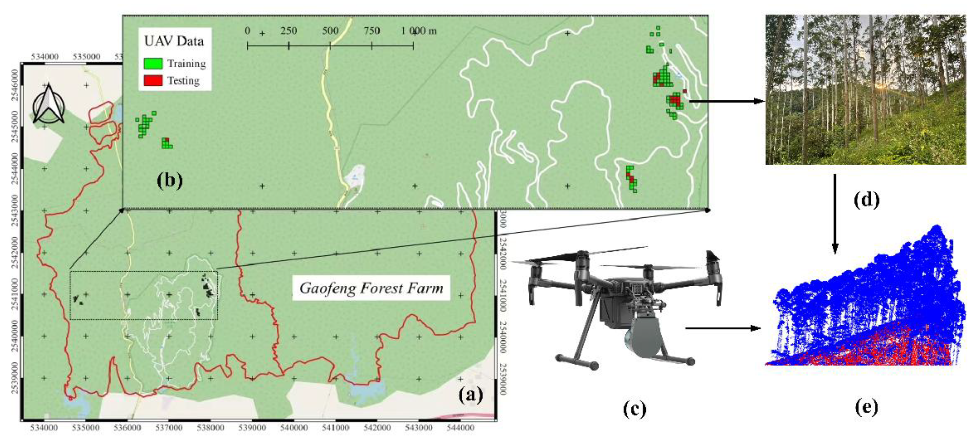
2.1. Study Area and UAV Data Collection

UAV LiDAR data used in this study were collected in Gaofeng Forest Farm of Nanning, Guangxi Province, China, in July of 2021. Gaofeng Forest Farm is a managed forest farm with dominant tree species of Eucalyptus robusta Smith, Castanopsis hystrix Miq., Cunninghamia lanceolata (Lamb.) Hook. and Magnolia denudata Desr., etc. The location and distribution of the UAV sample plots are within the extent of (108.338°–108.372°E, 22.9727°–22.9623°), as shown in Figure 1. The research area was 140–260 m above sea level with 0°–32° slope.

In the data collection campaign, a Genius Mini UAV LiDAR System of Beijing SureStar Technology Cooperation (https://www.isurestar.net, accessed on 30 July 2022) was carried by a DJI M210 multi rotor UAV platform (https://www.dji.com, accessed on 21 July 2022). The Genius Mini was set to a PRF (pulse repetition frequency) of 320 kHz and the UAV flying altitude above ground was around 100 m. Of the whole experiment, raw measurement data were collected, and the point cloud were processed by direct geo-referencing with POS (position and orientation) data. Intensity data were recorded per point.

2.2. Dataset Preparation

To generate a well-labeled training dataset and test dataset, we selected 87 tiles of 20 m × 20 m size from the UAV data which included 15,174,732 points in total. These selected 87 high-quality tiles contain different vegetation coverage and terrain condition. These high-quality data could help the network to learn the representative and essential features and for making informed judgments. Detailed information about the datasets are shown in Appendix A 

Table A1. Description of the UAV LiDAR dataset.

Forest Environment	Train Dataset				Test Dataset
	Mean Point Density (m−2)	Number of Tiles	Tree Species	Slope Range (°)	Mean Point Density (m−2)	Number of Tiles	Tree Species	Slope Range/(°)
Dense vegetation with flat terrain	793.22	9	Eucalyptus, Castanopsis	[0, 6.5]	955.74	3	Eucalyptus Magnolia	[0,5]
Dense vegetation with slope	684.48	35	Eucalyptus, Magnolia, Michelia	[10.5, 38]	610.38	8	Eucalyptus Castanopsis	[12.5, 33]
Sparse vegetation with flat terrain	201.01	8	Eucalyptus, bamboo	[0,7]	282.39	1	Eucalyptus	[0,0]
Sparse vegetation with slope	290.72	18	Eucalyptus, Chinese fir	[10,36]	370.17	5	Eucalyptus Michelia	[18,32]

. The automated method in the LAStools software (https://rapidlasso.com/lastools/, accessed on 21 July 2022) was used to filter the unclassified raw points to generate preliminary results, followed by further careful manual inspection. The point cloud visualization and editing tool in CloudCompare (v. 2.10.2; http://www.cloudcompare.org/, accessed on 20 July 2022) was used to visualize the cross section and manually label the points.

Then, the well-labeled data were split into the training dataset and test dataset. At this point, the 87 tiles were not split randomly since it is important to have representative samples that cover each kind of forest type and terrain conditions. The model was expected to learn as much diverse forest information as possible, and the test set covers a number of different forest environments in various situations. We follow the ratio of approximate 4:1 to divide the training (70 tiles) and test (17 tiles) sets.

Only the spatial coordinates [x, y, z] of the point cloud were preserved, and there were no additional features such as color or intensity. The reason is that it maximizes the model’s applicability to a wide range of sensors that may not be able to record the color or intensity, despite that some studies have shown that more features might improve the accuracy of recognition [44].

2.3. Additional Third-Party Dataset

We used UAV LiDAR data to train Terrain-net, while additional open datasets were also used to evaluate the model transfer ability. OpenGF [47] is a public ground filtering dataset which covers 47 km² and contains nine distinct representative terrain scenes of ALS point cloud from four different nations. We randomly selected three plots from the small city, village and mountain categories of the datasets for they contain forested environments in varying degrees. As shown in

Table 1. Details of selected plots from OpenGF.

Name	Land Type	Size/(m2)	Terrain Features and Tree Distribution
S4_4	Small City	500 × 500	Local undulating ground with many middle-size buildings and sparse tree distribution.
S6_23	Village	500 × 500	Natural ground with a few scattered buildings and large area of tree distribution.
S7_4	Mountain	500 × 500	Slope ground with dense vegetation

, the size of each plot is 500 m × 500 m, and the land type of each plot is different.

2.4. Terrain-Net Network Establishment

Terrain-net is a deep neural network that combines point convolution operator KPConv and self-attention to classify UAV LiDAR point cloud data into ground and non-ground types. Figure 2 shows the network architecture, which contains the input layer, the encoder, and the decoder. We briefly introduce the design of the architecture and the two core operations used in the network in detail below.

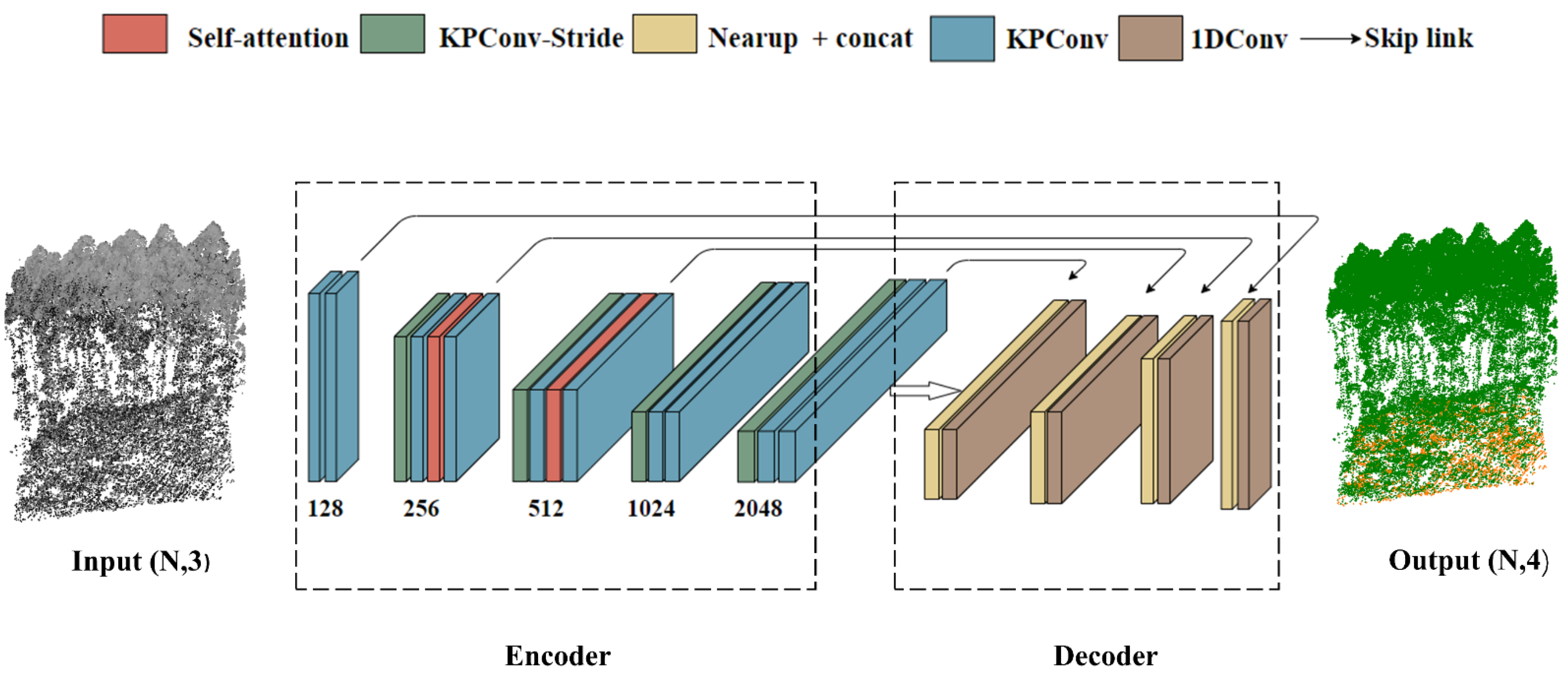
2.4.1. Terrain-Net Architecture

The Terrain-net architecture was based on KPConv architectures namely the KP-FCNN [43]. We kept the design of blocks as the original version. The input is an N × 3 matrix, where N represents the number of points and 3 means only the 3D coordinates were used.

In the encoder, Terrain-net mainly used two blocks, namely the KPConv and KPConv-stride. The KPConv block, which is described in the following Section 2.4.2, was used to extract pointwise features, and the KPConv-stride block was used to gradually increase the receptive field. There were five layers in the encoder. The first layer consisted of two KPConv blocks, and the subsequent layers consisted of a KPConv-stride block and two KPConv blocks. A self-attention block was also added in layer2 and layer3. Like the image networks which gradually decrease the size of the input image to expand the receptive field, the number of points was reduced progressively in the encoder, and the number of features increased in each layer accordingly. The dimensions of features in each layer were 128, 256, 512, 1024 and 2048, respectively.

The decoder had four layers, each one of which employs a nearest up-sampling block and a 1D convolution block. The skip links conveyed information between the layers in the encoder and decoder, which concatenated features to the up-sampling layer, then the output of the up-sampling layer was processed by the 1D convolution layer. In the decoder, the number of points increased progressively to revert to the original input shape, after which the output was composed with a label and each of the original input points. The dimensions of features in each layer were 1024, 512, 256, 128, respectively.

As is mentioned, KPConv can extract point-wise features well since it considers the neighborhood information, and it adopts a bottom-up feature extraction method and captures more information by gradually expanding its receptive field. Nevertheless, it lacks global information in the early stage, so we introduced self-attention to form a larger receptive field, which is further discussed in Section 2.4.3.

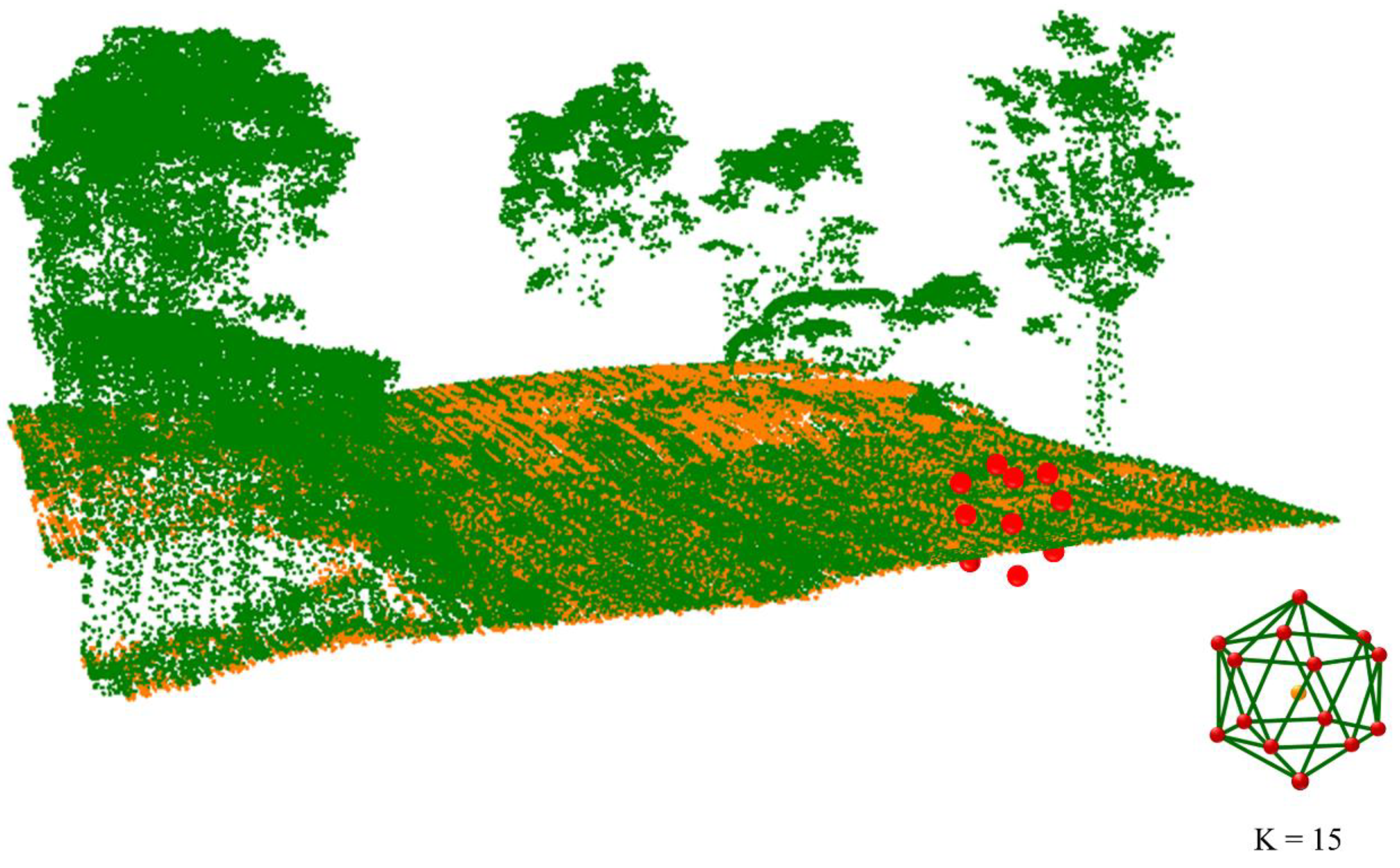
2.4.2. KPConv Point Convolution Operator

The KPConv operator, as one of the core techniques in Terrain-net, is a state-of-art design of point convolution that operates on point cloud without any intermediate representations [43]. Kernel weights of 2D image convolution are associated to the kernel pixels which are aligned with the pixel grid, and then discrete filters can be defined. Like 2D image convolution, KPConv extracts features in a 3D spherical neighborhood. The difference is that KPConv replaces kernel pixels by kernel points, to which the kernel weights are associated. The positions of kernel points are formulated as an optimization problem of the best coverage in the sphere space. Since input points are usually not aligned with kernel points, continuous filters are defined by using the correlation function to create a continuous domain. As a result, the feature of points is computed by multiplying all the kernel points’ weight, with their correlation to each kernel point. Figure 3 intuitively shows the kernel points of KPConv.

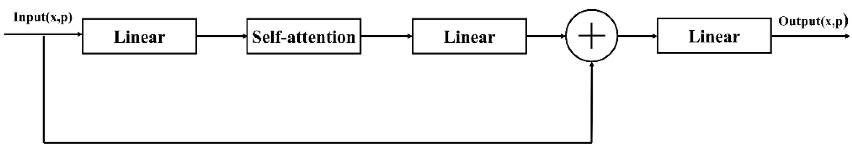
2.4.3. Self-Attention Operator

A general form of attention mechanism can be formulated as:

$$\mathrm{Attention}=f\left(g\left(x\right) ,x\right)$$

(1)

where $g\left(x\right)$ represents the adaptive weights, $x$ represents the input, and $f\left(g\left(x\right) ,x\right)$ represents how to combine the weights with the input. By using the attention mechanism, the adaptive weights could emphasize more important features, further improving the learning ability of the network. In Terrain-net, we designed a scalar self-attention block as shown in Figure 4:

A general scalar self-attention [15] can be described as in Equations (2) and (3):

$$g\left(x\right)=\mathrm{Softmax}\left( \phi \left(x\right) \psi {\left(x\right)}^T\right)$$

(2)

$$f\left(g\left(x\right), x\right)=g\left(x\right)\alpha \left(x\right)$$

(3)

where $\phi$ $,\psi ,$ $\alpha$ are pointwise feature transformations, i.e., MLP. Equation (3) represents the scalar self-attention. The scalar attention calculates the output of scalar product between features transformed by $\phi$ and $\psi$ is used as an attention weight for aggregating features transformed by $\alpha$. Due to the way of assigning weight, different feature channel shares the same weight. Figure 4 illustrates a residual self-attention block we constructed in Terrain-net. Its design ideas are based on [48]. The core operation of the self-attention block is in the self-attention layer, and the operation can be represented as in Equation (4):

$$y=x-\mathrm{Softmax}\left( \phi \left(x\right) \psi {\left(x\right)}^T\right)\alpha \left(x\right)$$

(4)

The input first goes through a linear projection for a better space encoding learning, after which it goes through a self-attention layer. Finally, the input passes another linear projection and is added with the original input. In the self-attention block, the inputs are weighted dynamically via a similarity function. Unlike the pooling operation or the convolutional operation, the weights used in the self-attention layer depend on the different similarities of the inner elements of the input vector rather than predetermined by their relative location like in KPConv. Self-attention has a low inductive bias which constructs a large space to freely explore the inherent characteristics of the input data, to achieve better performance and generalization. Moreover, this dynamic weighting process can capture the global contextual information which brings a new perspective to the feature extraction.

2.5. Model Training

In the modeling progress of Terrain-net, the number of kernel points of a rigid kernel 𝐾 = 15. The initial subsampling parameter 𝑑𝑙₀ was set to 0.08 m, the radius of influence 𝑅 = 3.0 m, based on the characteristic of UAV LiDAR point cloud. The model was trained using the cross-entropy loss and the momentum gradient descent optimizer is used to minimize the loss with a momentum of 0.98. The initial learning rate was set to 0.01 and declined exponentially by dividing it by 10 for every 100 epochs.

The following data augmentation methodologies were applied before training:

Anisotropic Scaling: The input point cloud was scaled separately in each dimension. The scaling factor was picked uniformly in [0.8, 1.2].

Vertical rotation: The point cloud was rotated with a random angle of [0, 2$\pi$], around the vertical axis.

Noise: The point coordinates were added with a gaussian noise to perturb their positions. To prevent losing too many details, the standard deviation of the noise was adjusted to a value smaller than 𝑑𝑙₀.

On a desktop computer with an Intel(R) Xeon(R) Gold 6330 CPU, 160 GB of RAM, and an NVIDIA RTX 3090 GPU with 24 GB VRAM, all training and testing were performed. It took 300 epochs to train for converging, taking approximately 16 h. The batch size was set to 8.

3. Results

In this part, we exhibit the performance metrics of the Terrain-net, the testing results of our own dataset and additional third-party dataset.

3.1. Performance Metrics

Type I, Type II, and Total errors are the widely used evaluation metrics of ground filtering [49]. These traditional measurements are replaced by comparable or similar metrics extensively utilized in current studies. Here, the performance metrics used are per-class recall, precision, IoU (Intersection over Union), F1-score, as well as the overall accuracy (OA), Kappa coefficient (Kp), and MIoU (Mean IoU) based on the confusion matrix. The computations are summarized in Appendix A 

Table A2. Confusion Matrix.

		Reference
		Non-ground (0)	Ground (1)
Prediction	Non-ground (0)	TN (True negative)	FN (False negative)
	Ground (1)	FP (False positive)	TP (True positive)

, and the calculation formulas of performance metrics are shown in Appendix A 

Table A3. Summary of calculation formulas for performance metrics.

Abbreviation	Meaning	Formula
OA	overall accuracy	$\frac{\mathrm{TP}+\mathrm{TN}}{\mathrm{TP}+\mathrm{TN}+\mathrm{FN}+\mathrm{FP}}$
RG	Recall of ground points	$\frac{\mathrm{TP}}{\mathrm{TP}+\mathrm{FN}}$
RNG	Recall of non-ground points	$\frac{\mathrm{TN}}{\mathrm{TN}+\mathrm{FP}}$
PG	Precision of ground points	$\frac{\mathrm{TP}}{\mathrm{TP}+\mathrm{FP}}$
PNG	Precision of non-ground points	$\frac{\mathrm{TN}}{\mathrm{TN}+\mathrm{FN}}$
IoUG	IoU of ground points	$\frac{\mathrm{TP}}{\mathrm{TP}+\mathrm{FN}+\mathrm{FP}}$
IoUNG	IoU of non-ground points	$\frac{\mathrm{TN}}{\mathrm{TN}+\mathrm{FN}+\mathrm{FP}}$
FG	F1-score of ground points	$2* \frac{{(\mathrm{R}}_{\mathrm{G}}{* \mathrm{P}}_{\mathrm{G}})}{{(\mathrm{R}}_{\mathrm{G}}{+\mathrm{P}}_{\mathrm{G}})}$
FNG	F1-score of non-ground points	$2* \frac{{(\mathrm{R}}_{\mathrm{NG}}{* \mathrm{P}}_{\mathrm{NG}})}{{(\mathrm{R}}_{\mathrm{NG}}{+\mathrm{P}}_{\mathrm{NG}})}$
MIoU	Mean value of IoUG and IoUNG	$\frac{{(\mathrm{Iou}}_{G }{+\mathrm{Iou}}_{\mathrm{NG}})}{2}$
Kp	Kappa coefficient	$\mathrm{P}0=\frac{\mathrm{TN}+\mathrm{TP}}{\mathrm{TP}+\mathrm{TN}+\mathrm{FP}+\mathrm{FN}}$ $\mathrm{P}\mathrm{c}=\frac{(\left(\mathrm{TN}+\mathrm{FN}\right)*\left(\mathrm{TN}+\mathrm{FP}\right)+\left(\mathrm{FN}+\mathrm{TP}\right)*(\mathrm{FP}+\mathrm{TP}))}{{(\mathrm{TP}+\mathrm{TN}+\mathrm{FP}+\mathrm{FN})}^2}$ $\mathrm{Kp}=\frac{(\mathrm{P}0-\mathrm{Pc})}{1-\mathrm{Pc}}$

. In general, the higher the evaluation metrics, the better the model performs.

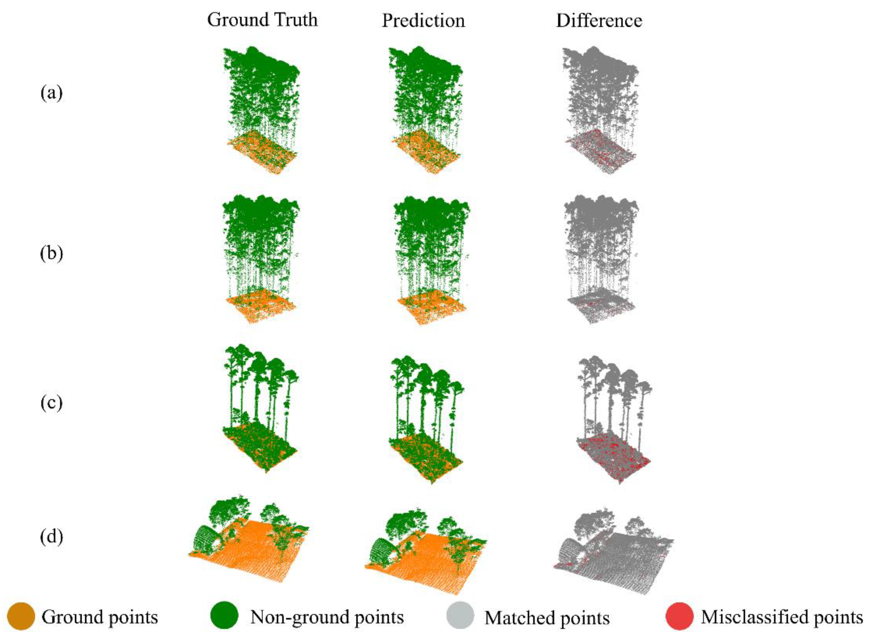
3.2. Evaluation Results of UAV Point Cloud

In this study, we selected four representative ground filtering algorithms. The slope-based algorithm, morphology-based algorithm and surface-based algorithm were implemented in Point Cloud Magic (PCM) software (v. 2.0.0 http://www.lidarcas.cn/soft, accessed on 20 July 2022), and the CSF algorithm was implemented in CloudCompare. In addition, we also trained the original KP-FCNN with the same training dataset of Terrain-net (70 tiles) and compared these methods with Terrain-net on the test dataset (17 tiles).

Table 2. Ground filtering results compared to traditional and deep learning algorithms on the test dataset.

Method	Ground				Non-Ground				Kp (%)	MIoU (%)	OA (%)
	Precision (%)	Recall (%)	F1-Score (%)	IoU (%)	Precision (%)	Recall (%)	F1-Score (%)	IoU (%)
Slope-based	75.2	98.5	84.8	74.5	99.4	88.5	93.2	88.1	78.6	81.3	91.5
Morphology-based	80.0	95.8	86.8	77.4	98.6	91.5	94.7	94.7	81.8	83.9	93.0
Surface-based	69.2	97.7	80.4	68.2	98.8	83.8	90.0	83.2	71.5	75.7	88.3
CSF	99.7	73.6	84.0	73.5	86.8	99.8	92.2	86.8	77.1	80.2	90.5
KP-FCNN	96.0	85.9	90.7	83.6	96.9	99.2	98.0	96.1	88.7	89.6	96.7
Terrain-net	95.5	92.9	94.2	89.0	98.6	99.1	98.8	97.7	93.0	93.3	98.0

shows the results of the ground filtering.

The results indicated among all sites, Terrain-net achieved the top mean Kp value (93.0%), followed by the original KP-FCNN, the morphology-based model, the slope-based model, CSF and the surface-based model. Meanwhile, the mean OA and MIoU of Terrain-net in all sites were the highest. The CSF achieved the highest ground precision and non-ground recall, while the slope-based model got the highest ground recall and non-ground precision. Nevertheless, Terrain-net was graded the highest F1-score of both two-point types. The highest F1-score indicated that Terrain-net performs well in both recall and precision, and the performance is well balanced.

Compared with the original KP-FCNN, Terrain-net improved performance on most metrics. In particular, the Kp was increased by 4.3%, the MIoU by 3.7% and the F1-score of ground by 3.7%. Compared to the best performing traditional algorithms (Morphology-based model) regarding the ground precision, Terrain-net increased the Kp by 11.2%, MIoU by 9.4% and the F1-score of ground by 7.4%. Ground filtering results of the Terrain-net on the test dataset are shown in Figure 5.

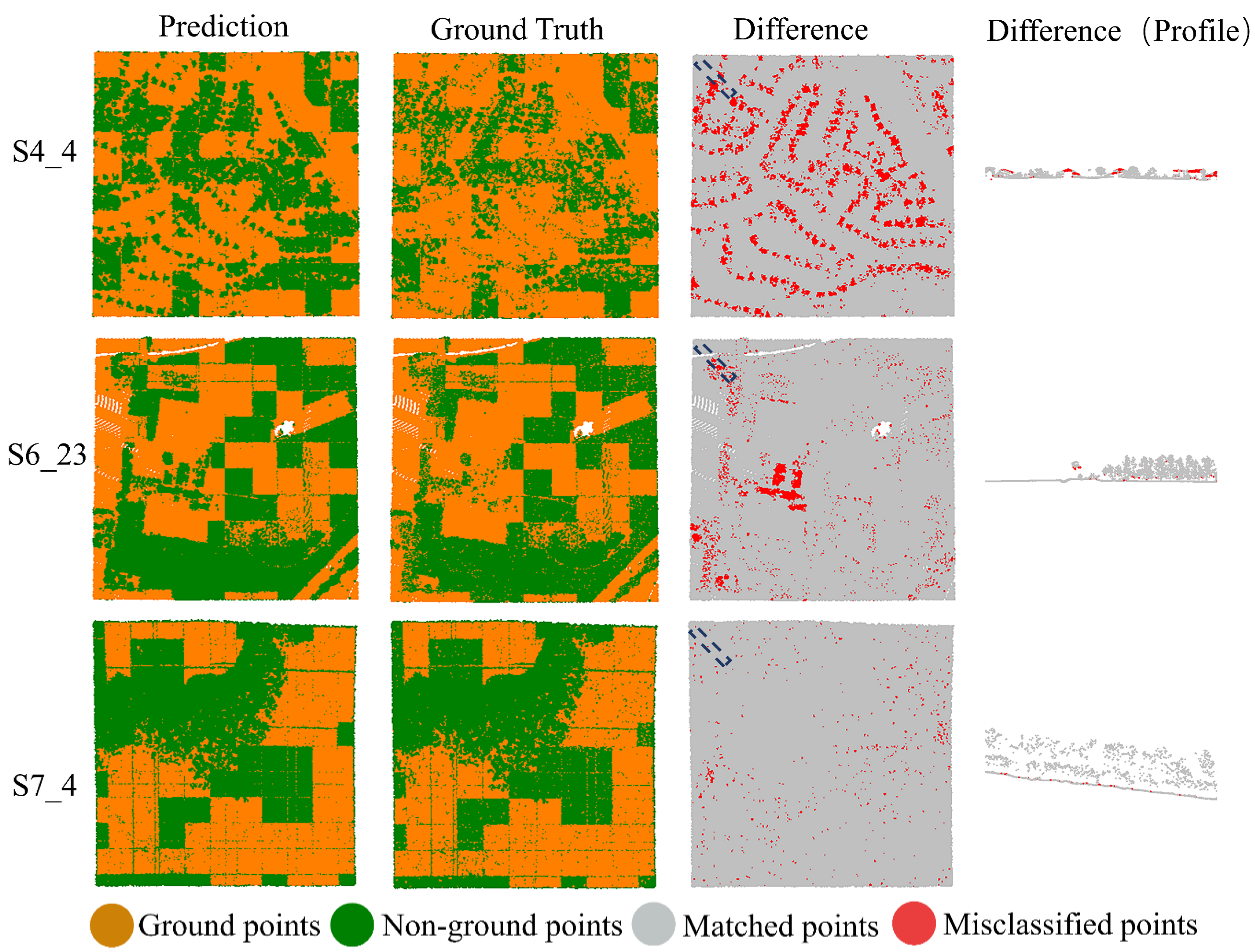
3.3. Evaluation Results of Additional Third-Party Dataset

To examine the generalization capability of Terrain-net in large scenes and other vegetated environments, we continued the evaluation with the OpenGF dataset and used its performance metrics reported in [47] including the Kappa coefficient and F1-score, excluding the Root Mean Square Error (RMSE) and approximate running time (ART). The results are shown in

Table 3. Ground filtering results on third-party public dataset.

Name	Ground		Non-Ground		OA (%)	Kp (%)
	IoU (%)	F1-Score (%)	IoU (%)	F1-Score (%)
S4_4	86.0	92.4	82.3	90.3	91.5	82.9
S6_23	92.8	96.3	94.6	97.2	96.6	93.5
S7_4	92.8	96.3	96.4	98.0	97.6	94.4

.

From the above results, it is clearly indicated that though Terrain-net was trained with UAV LiDAR data of 20 m × 20 m tiles in varying eucalyptus and fir forests environments with different terrain conditions, it performed quite well on ALS point cloud data in large-scale scenes (500 m × 500 m). It should be mentioned that (1) the OpenGF dataset covers scenarios including small cities, villages and mountain environments, the first two of which did not appear in the training dataset of Terrain-net at all, and (2) Terrain-net used UAV point cloud whose point density was much higher than that of ALS point cloud in OpenGF. These facts indicated that Terrain-net has remarkable generalization and robustness in transferring to varying sensors and data.

4. Discussion

4.1. Comparative Analyses with Traditional Methods and Models

Results in Table 2 indicated that Terrain-net performed the best regarding almost all the metrics except the ground recall and non-ground precision comparing to other traditional methods. The main reason may be that traditional methods are generally based on handcraft-designed rules and criteria to distinguish the ground and non-ground points, and the rules may not have the ability to fit the features of scenes not complied. The approach of Terrain-net learns the discrimination rules directly from the labeled point cloud via KPConv to capture delicate local information and combine with self-attention to capture long range interaction information. This technique of combining local and global feature extraction allows Terrain-net to learn more representative features. In addition, we also applied deep learning “tricks” such as residual connection and data augmentation, which further improved the feature extraction ability of Terrain-net.

The main errors of Terrain-net mainly concentrated in the junction part of trunks and the ground and at low vegetation locations. This is a challenging situation for point cloud ground filtering, and it is sometimes even difficult for humans to visually discriminate. Nevertheless, in most cases, Terrain-net can deliver good performance. It can also handle varying terrain conditions with steep slopes, gentle slopes or flat ground as shown in Figure 5.

4.2. Effectiveness Verification of Self-Attention

It can be found from the results (Table 2) that after adding the self-attention mechanism, the performance of Terrain-net became better than the original KP-FCNN. It is a consensus that there might be situations where deeper neural networks with more blocks can have stronger learning abilities with increased model parameters. To determine if the improvement came from the self-attention modification or just from the increment of the network depth, we conducted ablation experiments on this matter, by replacing the self-attention block in Terrain-net with old KPConv blocks. The results of ablation experiments are shown in

Table 4. The effectiveness of self-attention layer.

Model	Ground				Non-Ground				Kp (%)	MIoU (%)	OA (%)
	Precision (%)	Recall (%)	F1-Score (%)	IoU (%)	Precision (%)	Recall (%)	F1-Score (%)	IoU (%)
KP-FCNN (original)	96.0	85.9	90.7	83.6	96.9	99.2	98.0	96.1	88.7	89.6	96.7
KP-FCNN (more blocks)	99.1	83.6	90.7	83.0	96.1	99.8	97.9	96.0	88.7	89.5	96.6
Terrain-net	95.5	92.9	94.2	89.0	98.6	99.1	98.8	97.7	93.0	93.3	98.0

.

It can be observed that compared with the original KP-FCNN, the model with more KPConv blocks did not have significant improvements in overall indicators such as the Kp and MIoU. Although it had a significant improvement in ground precision, its ground recall decreased contrarily. Meanwhile, a section of ground points were identified as non-ground, which can be seen from the drop in the precision of non-ground points. Terrain-net exhibited the highest Kp, MIoU, OA, as well as the highest F1-scores of both ground and non-ground points. It indicated that Terrain-net had a more balanced performance in predicting ground and non-ground points. The reason why adding self-attention block is better than simply adding KPConv block might be that self-attention brings a new perspective of digging out spatial context. Adding a self-attention operation can be seen as a supplement to the convolution operation, helping to expand the receptive field of the convolution, which may allow the network to gain better understanding of the object being learned. In forest scenes, there are a plenty of larger objects like tall trees. Though KPConv gradually expands the receptive field during processing, adding self-attention can help to expand the receptive field in the early stage and capture more information of larger objects. Moreover, unlike KPConv which uses fixed weights assigned to the data, self-attention calculates dynamic weights to the data through the dot product from a global perspective, and the dynamic weights vary with inputs. This technique enables Terrain-net to better adapt to the complex and changing forest environment.

4.3. Selection of the Self-Attention Type and Variants

Section 4.2 showed that the added self-attention blocks play an indispensable role in the performance improvement of Terrain-net. In this section, we explored the design of different self-attention blocks and the impact of numbers of self-attention blocks on the performance of Terrain-net.

The self-attention includes two types of implementations. The self-attention layer is a key part of the self-attention block architecture, and its design may lead to different results. Here we first explored the different designs of the layer. Different self-attention type and their variants were adopted in the self-attention block. Part of their expressions are already given in Section 2.4.3, and the rest are given as follows:

$$y=x+\mathrm{Softmax}\left( \phi \left(x\right) \psi {\left(x\right)}^T\right)\alpha \left(x\right)$$

(5)

$$y=\mathrm{Softmax}\left( \phi \left(x\right)-\psi \left(x\right) \right)\odot \alpha \left(x\right)$$

(6)

$$y=x - \mathrm{Softmax}\left( \phi \left(x\right)-\psi \left(x\right) \right)\odot \alpha \left(x\right)$$

(7)

These self-attention blocks with different self-attention layers were placed in the same position in the network, i.e., the second and third layers of the Terrain-net. The corresponding results are shown in

Table 5. The effect of different self-attention block design.

Model	Ground				Non-Ground				Kp (%)	MIoU (%)	OA (%)
	Precision (%)	Recall (%)	F1-Score (%)	IoU (%)	Precision (%)	Recall (%)	F1-Score (%)	IoU (%)
Scalar attention (Equation (3))	96.7	91.2	93.9	88.5	98.1	99.3	98.7	97.5	92.6	93.0	96.7
Scalar attention (Equation (4))	95.5	92.9	94.2	89.0	98.6	99.1	98.8	97.7	93.0	93.3	98.0
Scalar attention (Equation (5))	95.5	92.4	94.0	88.6	98.4	99.1	98.7	97.6	92.7	93.1	97.8
Vector attention (Equation (6))	96.7	91.2	93.9	88.5	98.2	99.3	98.7	97.5	92.6	93.0	97.9
Vector attention (Equation (7))	91.7	95.5	93.5	87.8	99.1	98.3	98.7	97.5	92.2	92.6	97.9

. Compared with Equations (3)–(5), it represents another design of the self-attention layer. Equation (6) represents a vector self-attention [50], and Equation (7) represents a variant of the vector self-attention. We can see that different self-attention block designs did not bring significant differences to the final result. The overall performance of the self-attention block using Equation (4) was slightly better than those of the other formulas. No matter how the self-attention block was designed, the result was better than the original KP-FCNN. We did not add positional encoding to any design of self-attention layer. If positional encoding is added, according to the original work [50], the performance of blocks designed with vector self-attention may be improved.

The effect of different numbers of self-attention blocks on Terrain-net results was analyzed. Self-attention blocks can have different placement methods and can be added to different layers. In

Table 6. The effect of the number of self-attention block.

Model	Ground				Non-Ground				Kp (%)	MIoU (%)	OA (%)
	Precision (%)	Recall (%)	F1-Score (%)	IoU (%)	Precision (%)	Recall (%)	F1-Score (%)	IoU (%)
1 self-attention block	85.2	92.7	93.9	88.6	98.5	99.0	98.7	97.6	92.7	93.1	97.8
2 self-attention blocks	95.5	92.9	94.2	89.0	98.6	99.1	98.8	97.7	93.0	93.3	98.0
3 self-attention blocks	93.3	94.5	93.9	88.5	98.9	98.6	98.8	97.6	92.7	93.1	98.0
4 self-attention blocks	94.9	93.1	94.0	88.7	98.6	98.9	98.8	97.6	92.8	93.2	98.0
8 self-attention blocks	93.3	94.5	93.9	88.5	98.9	98.6	98.8	97.6	92.7	93.1	98.0

, the best results obtained from different positions after we fixed the increased number of self-attention blocks were listed. As the number of layers increases, the results did not improve significantly. This suggested the addition of two self-attention blocks to balance the model performance with respect to the number of parameters and the computation cost.

4.4. Model Transferring Performance

According to the results of Table 3, Terrain-net achieved the best result on site S7_4, which is mainly with slope ground and dense vegetation. The mountainous environment of S7_4 is the closest to our UAV data location, which could probably be the reason. Despite that the full coverage of S7_4 is 500 m × 500 m, much larger than the area of the training data and test data, Terrain-net can be well adapted to such large scenes. The main reason for errors may be from the different point density and observation geometry between ALS and UAV LiDAR. Terrain-net was not sensitive enough to the low vegetation points of ALS, because the they are normally much sparser than UAV points. Given the fact that Terrain-net was never trained with ALS data, we believe that it has performed beyond our expectations. As shown in Figure 6, the overall trend of the ground points was generally continuous, in line with the labeled ground, and there were no obvious misclassified points.

Compared with the excellent result of S7_4, the result of S4_4 was slightly inferior. The small city environment of S4_4 was quite different from our training data, and it contained local undulating ground with many middle-size buildings. According to the results, we can see that Terrain-net was relatively capable of recognizing locally discontinuous and undulating ground in S4_4, and it also labelled most vegetation points as non-ground very well. The fly in the ointment is that it was not good at recognizing the roofs of buildings which were mislabeled as ground. Since Terrain-net has not observed such small urban environment like S4_4 yet, it is no wonder to find these errors. It reminds us that data from more environments to be included in the training progress might expand the applicability of Terrain-net.

The performance of Terrain-net was relatively good in site S6_23, which is mainly located in a village environment. It had fewer buildings and more vegetation compared with S4_4 and had flatter terrain than S7_7, but it still had discontinuous and undulating terrain. Its errors were mainly concentrated in cases that recognize roofs as ground, and there were misclassifications at the junction part of vegetation and ground.

In general, the results provided clear evidence that, for a deep neural network approach to classify point cloud, the raw observation is part of the key to strengthen the transferring ability of the network. Data never being observed are not necessarily treated with poor determination, as long as their inner characteristics have certain connections with the ones being observed. Terrain-net transforms features of trees in UAV data to trees in ALS data, then it can find the trees in ALS data of mountains and villages. However, it is not capable of transforming features from trees to buildings in its current state. Evolutions will be possible if it is fed with more data from new environments.

5. Conclusions

In this study, we designed an end-to-end network, namely Terrain-net, for UAV ground point filtering in forested environments. This method combines a state-of-the-art point convolution KPConv and self-attention. It used well-labeled points which contained varying forest environments for training and testing. Comparing to classical algorithms, Terrain-net achieved the best performance. Furthermore, Terrain-net was evaluated with ALS data to perform remarkably in other environments, such as a small city, a village and a mountain, indicating good generalization ability and robustness. We believe that the network can be a useful tool for UAV ground point filtering tasks.

In the future work we hope to further construct this point cloud deep learning tool, by adding training data collected by multiple sensors from various terrains and scenes to increase the model generalization capability. The current model, code and documentation of Terrain-net is available at https://github.com/bjfu-lidar/Terrain-net (accessed on 11 November 2022). We would like to build up an open source, easy-to-use toolset for people to use.

References

1. Pearce, D.W. The Economic Value of Forest Ecosystems. Ecosyst. Health 2001, 7, 284–296. [Google Scholar] [CrossRef] [Green Version]
2. Zimble, D.A.; Evans, D.L.; Carlson, G.C.; Parker, R.C.; Grado, S.C.; Gerard, P.D. Characterizing Vertical Forest Structure Using Small-Footprint Airborne LiDAR. Remote Sens. Environ. 2003, 87, 171–182. [Google Scholar] [CrossRef] [Green Version]
3. Krisanski, S.; Taskhiri, M.S.; Turner, P. Enhancing Methods for Under-Canopy Unmanned Aircraft System Based Photogrammetry in Complex Forests for Tree Diameter Measurement. Remote Sens. 2020, 12, 1652. [Google Scholar] [CrossRef]
4. Guo, Q.; Su, Y.; Hu, T.; Guan, H.; Jin, S.; Zhang, J.; Zhao, X.; Xu, K.; Wei, D.; Kelly, M.; et al. Lidar Boosts 3D Ecological Observations and Modelings: A Review and Perspective. IEEE Geosci. Remote Sens. Mag. 2021, 9, 232–257. [Google Scholar] [CrossRef]
5. Hu, X.; Yuan, Y.; Shan, J.; Hyyppä, J.; Waser, L.T.; Li, X.; Thenkabail, P.S. Deep-Learning-Based Classification for DTM Extraction from ALS Point Cloud. Remote Sens. 2016, 8, 730. [Google Scholar] [CrossRef] [Green Version]
6. Vosselman, G. Slope Based Filtering of Laser Altimetry Data. Int. Arch. Photogramm. Remote Sens. 2000, 33, 935–942. [Google Scholar]
7. Meng, X.; Wang, L.; Silván-Cárdenas, J.L.; Currit, N. A Multi-Directional Ground Filtering Algorithm for Airborne LIDAR. ISPRS J. Photogramm. Remote Sens. 2009, 64, 117–124. [Google Scholar] [CrossRef] [Green Version]
8. Wang, C.K.; Tseng, Y.H. Dem Generation from Airborne Lidar Data by an Adaptive Dual-Directional Slope Filter. Int. Arch. Photogramm. Remote Sens. Spat. Inf. Sci. 2010, 38, 628–632. [Google Scholar]
9. Sithole, G.; Vosselman, G. Filtering of Airborne Laser Scanner Data Based on Segmented Point Clouds. Int. Arch. Photogramm. Remote Sens. Spat. Inf. Sci. 2005, 36, W19. [Google Scholar]
10. Zhang, K.; Chen, S.C.; Whitman, D.; Shyu, M.L.; Yan, J.; Zhang, C. A Progressive Morphological Filter for Removing Nonground Measurements from Airborne LIDAR Data. IEEE Trans. Geosci. Remote Sens. 2003, 41, 872–882. [Google Scholar] [CrossRef] [Green Version]
11. Chen, Q.; Gong, P.; Baldocchi, D.; Xie, G. Filtering Airborne Laser Scanning Data with Morphological Methods. Photogramm. Eng. Remote Sens. 2007, 73, 175–185. [Google Scholar] [CrossRef] [Green Version]
12. Axelsson, P. DEM Generation from Laser Scanner Data Using Adaptive TIN Models. Int. Arch. Photogramm. Remote Sens. 2000, 23, 110–117. [Google Scholar]
13. Kraus, K.; Pfeifer, N. Determination of Terrain Models in Wooded Areas with Airborne Laser Scanner Data. ISPRS J. Photogramm. Remote Sens. 1998, 53, 193–203. [Google Scholar] [CrossRef]
14. Zhang, W.; Qi, J.; Wan, P.; Wang, H.; Xie, D.; Wang, X.; Yan, G. An Easy-to-Use Airborne LiDAR Data Filtering Method Based on Cloth Simulation. Remote Sens. 2016, 8, 501. [Google Scholar] [CrossRef]
15. Vaswani, A.; Shazeer, N.; Parmar, N.; Uszkoreit, J.; Jones, L.; Gomez, A.N.; Kaiser, Ł.; Polosukhin, I. Attention Is All You Need. In Proceedings of the Advances in Neural Information Processing Systems, Long Beach, CA, USA, 4–9 December 2017; Volume 2017. [Google Scholar]
16. Devlin, J.; Chang, M.W.; Lee, K.; Toutanova, K. BERT: Pre-Training of Deep Bidirectional Transformers for Language Understanding. In Proceedings of the 2019 Conference of the North American Chapter of the Association for Computational Linguistics: Human Language Technologies (NAACL HLT 2019), Minneapolis, MN, USA, 2–7 June 2019; Volume 1. [Google Scholar]
17. Liu, Z.; Lin, Y.; Cao, Y.; Hu, H.; Wei, Y.; Zhang, Z.; Lin, S.; Guo, B. Swin Transformer: Hierarchical Vision Transformer Using Shifted Windows. In Proceedings of the IEEE International Conference on Computer Vision, Montreal, QC, Canada, 10–17 October 2021. [Google Scholar]
18. Yi, L.; Su, H.; Guo, X.; Guibas, L. SyncSpecCNN: Synchronized Spectral CNN for 3D Shape Segmentation. In Proceedings of the 30th IEEE Conference on Computer Vision and Pattern Recognition (CVPR 2017), Honolulu, HI, USA, 21–26 July 2016; Volume 2017, pp. 2282–2290. [Google Scholar]
19. Xu, Y.; Fan, T.; Xu, M.; Zeng, L.; Qiao, Y. SpiderCNN: Deep Learning on Point Sets with Parameterized Convolutional Filters. In Lecture Notes in Computer Science (Including Subseries Lecture Notes in Artificial Intelligence and Lecture Notes in Bioinformatics); Springer: Cham, Switzerland, 2018; Volume 11212 LNCS, pp. 87–102. [Google Scholar]
20. Zhao, H.; Jiang, L.; Fu, C.W.; Jia, J. Pointweb: Enhancing Local Neighborhood Features for Point Cloud Processing. In Proceedings of the IEEE Computer Society Conference on Computer Vision and Pattern Recognition, Long Beach, CA, USA, 15–20 June 2019; Volume 2019, pp. 5565–5573. [Google Scholar]
21. Maturana, D.; Scherer, S. VoxNet: A 3D Convolutional Neural Network for Real-Time Object Recognition. In Proceedings of the IEEE International Conference on Intelligent Robots and Systems, Hamburg, Germany, 28 September–3 October 2015; Volume 2015, pp. 922–928. [Google Scholar]
22. Li, Y.; Bu, R.; Sun, M.; Wu, W.; Di, X.; Chen, B. PointCNN: Convolution On X-Transformed Points. In Advances in Neural Information Processing Systems; Bengio, S., Wallach, H., Larochelle, H., Grauman, K., Cesa-Bianchi, N., Garnett, R., Eds.; Curran Associates, Inc.: Red Hook, NY, USA, 2018; Volume 31. [Google Scholar]
23. Simonovsky, M.; Komodakis, N. Dynamic Edge-Conditioned Filters in Convolutional Neural Networks on Graphs. In Proceedings of the Proceedings of the IEEE Conference on Computer Vision and Pattern Recognition, Honolulu, HI, USA, 21–26 July 2017; pp. 3693–3702. [Google Scholar]
24. Qi, Y.; Dong, X.H.; Chen, P.; Lee, K.H.; Lan, Y.; Lu, X.; Jia, R.; Deng, J.; Zhang, Y. Canopy Volume Extraction of Citrus Reticulate Blanco Cv. Shatangju Trees Using UAV Image-Based Point Cloud Deep Learning. Remote Sens. 2021, 13, 3437. [Google Scholar] [CrossRef]
25. Chen, J.; Chen, Y.; Liu, Z. Classification of Typical Tree Species in Laser Point Cloud Based on Deep Learning. Remote Sens. 2021, 13, 4750. [Google Scholar] [CrossRef]
26. Xu, L.; Zheng, S.; Na, J.; Yang, Y.; Mu, C.; Shi, D. A Vehicle-Borne Mobile Mapping System Based Framework for Semantic Segmentation and Modeling on Overhead Catenary System Using Deep Learning. Remote Sens. 2021, 13, 4939. [Google Scholar] [CrossRef]
27. Widyaningrum, E.; Bai, Q.; Fajari, M.K.; Lindenbergh, R.C. Airborne Laser Scanning Point Cloud Classification Using the Dgcnn Deep Learning Method. Remote Sens. 2021, 13, 859. [Google Scholar] [CrossRef]
28. Sun, C.; Zhang, F.; Zhao, P.; Zhao, X.; Huang, Y.; Lu, X. Automated Simulation Framework for Urban Wind Environments Based on Aerial Point Clouds and Deep Learning. Remote Sens. 2021, 13, 2383. [Google Scholar] [CrossRef]
29. Chen, Y.; Liu, X.; Xiao, Y.; Zhao, Q.; Wan, S. Three-Dimensional Urban Land Cover Classification by Prior-Level Fusion of Lidar Point Cloud and Optical Imagery. Remote Sens. 2021, 13, 4928. [Google Scholar] [CrossRef]
30. Rizaldy, A.; Persello, C.; Gevaert, C.M.; Oude Elberink, S.J. Fully Convolutional Networks for Ground Classification from Lidar Point Clouds. ISPRS Ann. Photogramm. Remote Sens. Spat. Inf. Sci. 2018, 4, 8. [Google Scholar] [CrossRef] [Green Version]
31. Yang, Z.; Tan, B.; Pei, H.; Jiang, W. Segmentation and Multi-Scale Convolutional Neural Network-Based Classification of Airborne Laser Scanner Data. Sensors 2018, 18, 3347. [Google Scholar] [CrossRef] [Green Version]
32. Schmohl, S.; Sörgel, U. Submanifold Sparse Convolutional Networks for Semantic Segmentation of Large-Scale ALS Point Clouds. ISPRS Ann. Photogramm. Remote Sens. Spatial Inf. Sci. 2019, IV-2/W5, 77–84. [Google Scholar] [CrossRef] [Green Version]
33. Yotsumata, T.; Sakamoto, M.; Satoh, T. Quality Improvement for Airborne Lidar Data Filtering Based on Deep Learning Method. Int. Arch. Photogramm. Remote Sens. Spat. Inf. Sci. 2020, 43, 355–360. [Google Scholar] [CrossRef]
34. Nurunnabi, A.; Teferle, F.N.; Li, J.; Lindenbergh, R.C.; Hunegnaw, A. An Efficient Deep Learning Approach for Ground Point Filtering in Aerial Laser Scanning Point Clouds. Int. Arch. Photogramm. Remote Sens. Spat. Inf. Sci. 2021, 43, 1–8. [Google Scholar] [CrossRef]
35. Janssens-Coron, E.; Guilbert, E. Ground Point Filtering from Airborne Lidar Point Clouds Using Deep Learning: A Preliminary Study. Int. Arch. Photogramm. Remote Sens. Spat. Inf. Sci. 2019, 42, 1559–1565. [Google Scholar] [CrossRef] [Green Version]
36. Qi, C.R.; Su, H.; Mo, K.; Guibas, L.J. PointNet: Deep Learning on Point Sets for 3D Classification and Segmentation. In Proceedings of the 30th IEEE Conference on Computer Vision and Pattern Recognition (CVPR 2017), Honolulu, HI, USA, 21–26 July 2016; Volume 2017, pp. 652–660. [Google Scholar]
37. Jin, S.; Su, Y.; Zhao, X.; Hu, T.; Guo, Q. A Point-Based Fully Convolutional Neural Network for Airborne LiDAR Ground Point Filtering in Forested Environments. IEEE J. Sel. Top. Appl. Earth Obs. Remote Sens. 2020, 13, 3958–3974. [Google Scholar] [CrossRef]
38. Krisanski, S.; Taskhiri, M.S.; Aracil, S.G.; Herries, D.; Turner, P. Sensor Agnostic Semantic Segmentation of Structurally Diverse and Complex Forest Point Clouds Using Deep Learning. Remote Sens. 2021, 13, 1413. [Google Scholar] [CrossRef]
39. Qi, C.R.; Yi, L.; Su, H.; Guibas, L.J. PointNet++: Deep Hierarchical Feature Learning on Point Sets in a Metric Space. In Proceedings of the Advances in Neural Information Processing Systems, Long Beach, CA, USA, 4–9 December 2017; Volume 2017. [Google Scholar]
40. Huang, S.; Liu, L.; Dong, J.; Fu, X.; Huang, F. SPGCN: Ground Filtering Method Based on Superpoint Graph Convolution Neural Network for Vehicle LiDAR. J. Appl. Remote Sens. 2022, 16. [Google Scholar] [CrossRef]
41. Chen, L.; Chen, W.; Xu, Z.; Huang, H.; Wang, S.; Zhu, Q.; Li, H. DAPnet: A Double Self-Attention Convolutional Network for Point Cloud Semantic Labeling. IEEE J. Sel. Top. Appl. Earth Obs. Remote Sens. 2021, 14, 3958–3974. [Google Scholar] [CrossRef]
42. Soilán, M.; Nóvoa, A.; Sánchez-Rodríguez, A.; Riveiro, B.; Arias, P. Semantic Segmentation of Point Clouds with Pointnet and Kpconv Architectures Applied to Railway Tunnels. ISPRS Ann. Photogramm. Remote Sens. Spat. Inf. Sci. 2020, 5, 281–288. [Google Scholar] [CrossRef]
43. Thomas, H.; Qi, C.R.; Deschaud, J.-E.; Marcotegui, B.; Goulette, F.; Guibas, L.J. Kpconv: Flexible and Deformable Convolution for Point Clouds. In Proceedings of the IEEE/CVF International Conference on Computer Vision, Seoul, Korea, 27 October–2 November 2019; pp. 6411–6420. [Google Scholar]
44. Kada, M.; Kuramin, D. ALS Point Cloud Classification Using Pointnet++ and KPCONV with Prior Knowledge. Int. Arch. Photogramm. Remote Sens. Spat. Inf. Sci. 2021, 46, 91–96. [Google Scholar] [CrossRef]
45. Huang, Z.; Wang, X.; Wei, Y.; Huang, L.; Shi, H.; Liu, W.; Huang, T.S. CCNet: Criss-Cross Attention for Semantic Segmentation. IEEE Trans. Pattern Anal. Mach. Intell. 2020. [Google Scholar] [CrossRef] [PubMed]
46. Wang, X.; Girshick, R.; Gupta, A.; He, K. Non-Local Neural Networks. In Proceedings of the IEEE Computer Society Conference on Computer Vision and Pattern Recognition, Salt Lake, UT, USA, 18–23 June 2018. [Google Scholar]
47. Qin, N.; Tan, W.; Ma, L.; Zhang, D.; Li, J. OpenGF: An Ultra-Large-Scale Ground Filtering Dataset Built upon Open ALS Point Clouds around the World. In Proceedings of the IEEE Computer Society Conference on Computer Vision and Pattern Recognition Workshops, Nashville, TN, USA, 19–25 June 2021. [Google Scholar]
48. Guo, M.H.; Cai, J.X.; Liu, Z.N.; Mu, T.J.; Martin, R.R.; Hu, S.M. PCT: Point Cloud Transformer. Comput. Vis. Media 2021, 7, 187–199. [Google Scholar] [CrossRef]
49. Meng, X.; Currit, N.; Zhao, K. Ground Filtering Algorithms for Airborne LiDAR Data: A Review of Critical Issues. Remote Sens. 2010, 2, 833–860. [Google Scholar] [CrossRef]
50. Zhao, H.; Jiang, L.; Jia, J.; Torr, P.H.S.; Koltun, V. Point Transformer. In Proceedings of the IEEE/CVF International Conference on Computer Vision, Montreal, QC, Canada, 10–17 October 2021; pp. 16259–16268. [Google Scholar]
Figure 1. Illustration of the forest farm location (a), the distribution of the UAV LiDAR data tiles (b), the model diagram of the UAV LiDAR scanner and the UAV platform carrying the LiDAR (c), the picture of the real forest plots (d), and a sample of the UAV point cloud (e).
Remotesensing 14 05798 g001
Figure 2. The structure of Terrain-net. The encoder part and decoder part were marked by dashed boxes.
Remotesensing 14 05798 g002
Figure 3. Illustration of how the KPConv interacts with the point cloud. Bottom right corner of the picture shows the position of the kernel points in the sphere.
Remotesensing 14 05798 g003
Figure 4. The detailed structure design of the self-attention module. The linear box represents a two-layer MLP. The Self-attention box represents the modified self-attention layer.
Remotesensing 14 05798 g004
Figure 5. Ground filtering result of the Terrain-net on test dataset. The four representative forest environment types in the dataset are shown from (ad), in order: dense vegetation with slope, dense vegetation with flat terrain, sparse vegetation with slope, and sparse vegetation with flat terrain.
Remotesensing 14 05798 g005
Figure 6. Ground filtering results of the Terrain-net on an additional third-party dataset. The dashed box in the Difference map indicates the location of Difference (Profile).
Remotesensing 14 05798 g006