Article

Assessment of Permeability Windbreak Forests with Different Porosities Based on Laser Scanning and Computational Fluid Dynamics

1
Beijing Key Laboratory of Precise Forestry, Beijing Forestry University, Beijing 100083, China
2
Institute of GIS, RS & GPS, Beijing Forestry University, Beijing 100083, China
*
Author to whom correspondence should be addressed.
Remote Sens. 2022, 14(14), 3331; https://doi.org/10.3390/rs14143331
Submission received: 17 May 2022 / Revised: 23 June 2022 / Accepted: 4 July 2022 / Published: 11 July 2022
(This article belongs to the Special Issue Application of LiDAR Point Cloud in Forest Structure)

Abstract

:
Accurate modeling of windbreaks is essential for the precise assessment of wind protection performance. However, in most windbreak studies, the models used the approximate shape of the simulated trees, resulting in significant differences between the simulated results and the actual situation. In this study, terrestrial laser scanning (TLS) was used to extract tree parameters, which were used in a quantitative structural model (AdQSM) to recreate the tree structure and restore the wind field environment using the computational fluid dynamics software PHOENICS. In addition, we compared the bias, precision, and accuracy of porosity of Ginkgo biloba (with elliptical crown) and Populus alba (with conical crown), which have been commonly used in previous windbreak studies. The results showed that AdQSM has a high reduction rate and ability to reproduce the field conditions of the study area. After wind field simulation, the wind speed root mean square errors of the point cloud model at three heights (3, 6, and 9 m) were 0.272, 0.377, and 0.437 m/s, respectively, and the wind speed correlation coefficients r were 0.967, 0.965, and 0.937, respectively, which were significantly more accurate than those of the remaining two structures. Finally, the porosity of the windbreak forest obtained using the modeled sample plot showed a higher correlation with the wind permeability coefficient than that obtained using the existing approach. Windbreak models with three different porosities under the same conditions had different effects on the wind environment, particularly the location of the maximum wind speed reduction, variation of wind speed with porosity, and recovery rate of leeward wind speed. TLS can accurately extract windbreak factors and calculate the porosity, thus greatly improving the reliability of windbreak effect research in windbreak forests. This study provides a promising direction for future research related to the simulation of windbreak effects in windbreak forests.

Graphical Abstract

1. Introduction

Agricultural windbreaks are considered green barriers that can prevent land desertification and protect crops from wind and sand, especially in areas with mixed agriculture and livestock [1]. At the same time, wind, water, sand, and natural disasters such as drought are the main factors affecting agricultural production. To improve the ecological environment and mitigate natural disasters, the Chinese government has implemented a series of ecological restoration projects such as the Three North Windbreak Forest Project and the Grain Retirement Project [2].
Tree structural parameters determine the canopy and stem properties under windy conditions [3], which are important factors affecting their effectiveness in protecting trees from wind. The accurate determination of structural parameters of windbreak forests and their accurate modeling are of great significance in assessing the effectiveness of windbreak forests. As terrestrial laser scanning (TLS) has become more accurate, its ability to capture 3D space [4] has also improved. TLS is becoming an increasingly popular tool in forest management, agricultural production, and ecological studies [5], tree parameters such as porosity, tree volume, leaf area density [6], breast height, tree diameter, and crown width, extracted from TLS data [7,8,9], no longer require manual measurement. In addition, the use of point cloud data for tree species classification is becoming increasingly useful for providing information to support forest mapping and inventory [10]. The generation of 3D point clouds by TLS allows the quantitative analysis of trees and reconstruction of 3D tree models. TLS point cloud data modeling with AdQSM has the following advantages: (1) accuracy: tree and stand characteristics such as position, height, canopy cover, species, and trunk curve can be measured, and the corresponding parts of an individual tree can be described accurately and in detail, giving their position, size, orientation, and relationship with other trees [11,12]; (2) digital: with ease of storing and managing datasets, any attribute can be extracted at any time after the construction is completed without using the actual data and most of the relevant information from the original data is retained in a digital form for future use; (3) automatic: no manual operation is required, allowing pipeline processing of a large number of trees being tested; and (4) fast: single trees can be modeled almost immediately (within tens of seconds).
Over the past few years, most studies conducted on windbreak forests have modeled the resistance of the canopy as a homogeneous porous region, using approximate models, rather than the real shape of the trees [13]. This does not accurately reflect the 3D turbulent flow characteristics. The canopy structure in computational fluid dynamics (CFD) is specified by the leading-edge area density, and this information is required for each grid point in the 3D computational domain. In previous studies, some scholars saw the whole windbreak as a 2D artificial obstacle with a simple geometry, such as a flat surface with round holes and an industrial metal screen [14,15]. Lopez et al. synthesized an actual 3D tree model from a single image, integrating 2D or 3D trees as shapes directly from a sparse set of images into the modeling process, requiring only labeling of leaves, trunk, and a few branch areas [16]. However, the limitations arising from this approach are that, for natural windbreak strips and most artificial windbreak strips, the boundaries are complex, and it is difficult to recover the status quo. This has a significant impact on the accurate simulation of windbreak effects because it does not reflect the true condition of trees. Some researchers have studied the airflow of a 3D windbreak forest composed of cypress trees, each with a conical crown, modeling the resistance of the canopy as a uniformly porous area [17]. As the porosity is fixed, their established model of a regular cone can only be used for one type of tree and is not universally applicable [18]. It is difficult to simulate agricultural windbreaks comprising irregularly shaped trees. Most of the recent studies have used numerical simulations and wind tunnel experiments to assess the wind field distribution in windbreak forests in the presence of high winds [19,20]. These studies simulated windbreaks in their natural state using plant models at different scales [21,22]. However, the dynamic complexity of forest structures under field conditions cannot be controlled as in wind tunnel environments or simulation studies. Therefore, indirect methods, such as the TLS technique, have been used more widely to determine the forest fraction structure in applications where extended regions need to be described with high accuracy [23].
The purpose of this study was to propose a new method for windbreak forest research by performing a 3D reconstruction of TLS data to improve the accuracy of simulations and then conduct a wind field simulation to accurately assess its windbreak effect [24]. The wind velocity data measured in the field were combined with canopy models approximated from previous studies for comparison and accuracy verification. This study paves the way for a new wind protection effect simulation for agricultural windbreak forests.

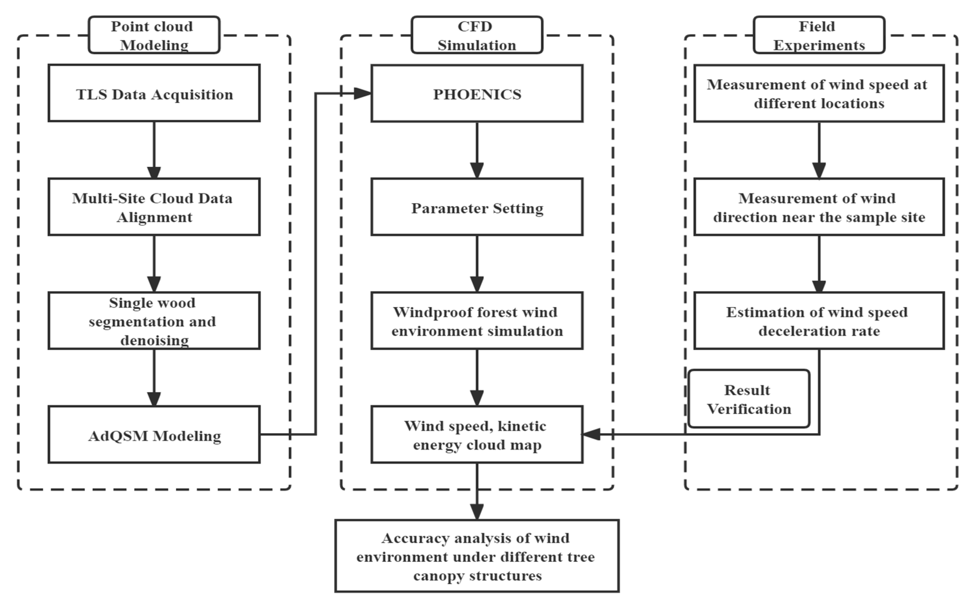
2. Materials and Methods

The porosity because of different canopy structures varies greatly, and the obstructive effect on airflow differs. Therefore, we compared the wind protection effects of windbreaks with respect to wind; particularly, the permeability performance of canopy structures with different porosities. The experimental steps to complete this study were as follows: (a) extraction of the protective forest parameters using TLS and modeling by AdQSM, the modeling software Blender was used to mimic the canopy of ginkgo and poplar trees to create oval and conical models; (b) importing the protective forest model into the CFD software PHOENICS for wind field simulation; and (c) comparing and analyzing the simulation results of tree crowns with different porosities and selecting the best crown model. The complete workflow is illustrated in Figure 1.

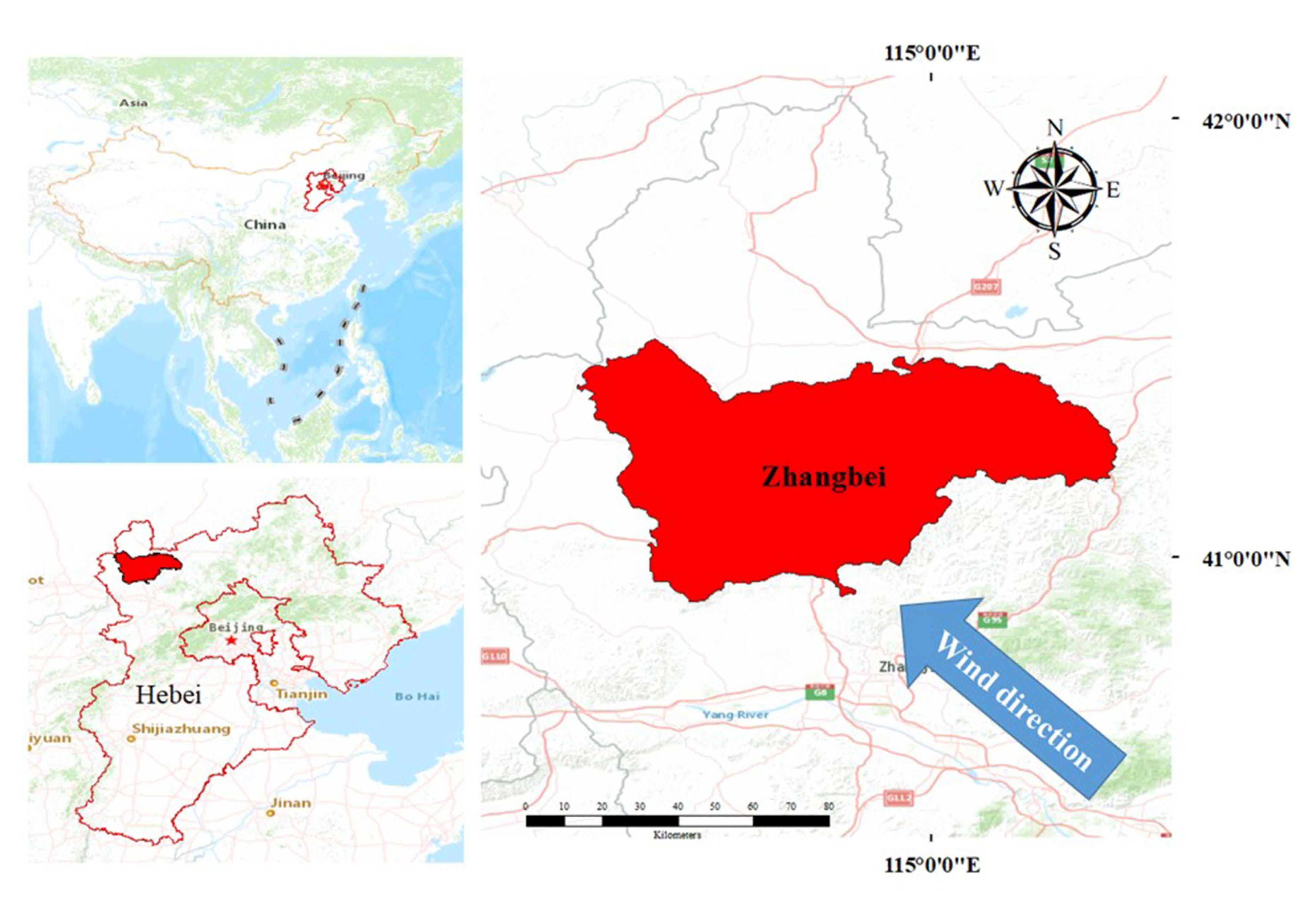
2.1. Selection of the Study Area

Three criteria were used to select the study area: (a) windbreak tree species should be representative of other similar area species; (b) windbreaks should be located away from villages, towns, and other residential areas to avoid blockage of airflow; and (c) local wind and sand hazards should be serious and frequent in the area.
Taking all of these factors into consideration, we chose Zhangbei County, Hebei Province, China (40.48–42.47°N, 113.54–118°E). The region has a mid-temperate continental monsoon climate with arid, windy, and low rainfall with a mean annual temperature of 2–6 °C, and the mean annual precipitation is approximately 300 mm. The study area was a double-row windbreak forest, 30 m long and 5 m wide, located between agricultural fields, with flat terrain and poplar trees. The surrounding crops were mainly oats and cabbages.

2.2. Data Acquisition

2.2.1. Acquisition of Sample Plot Inventory Data

A double-row windbreak forest was selected, and the locations of individual trees (including latitude and longitude coordinates) were recorded to measure tree height, diameter at breast height, and crown spacing. The health status of each tree was also recorded. The actual situation is shown in Table 1.

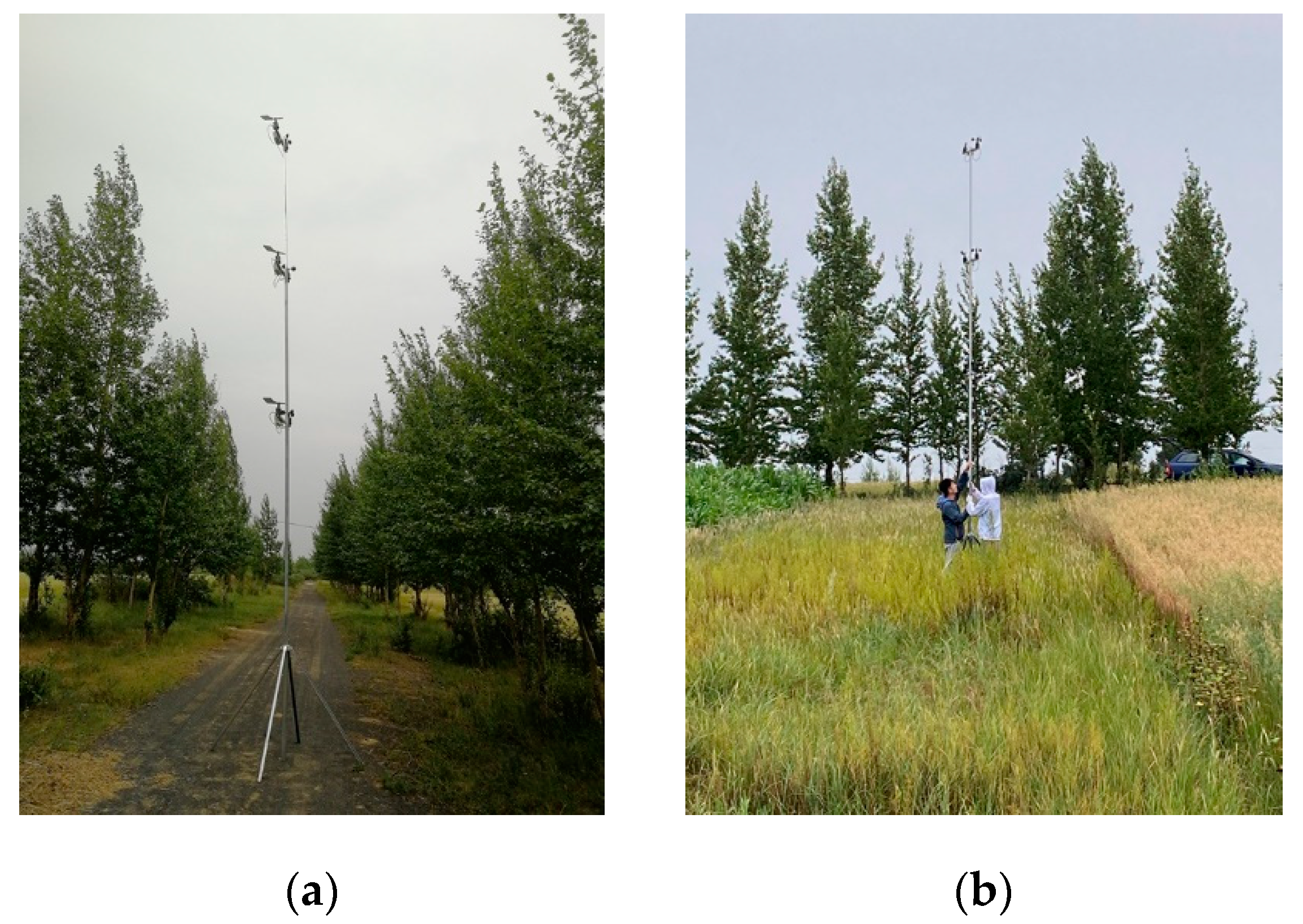
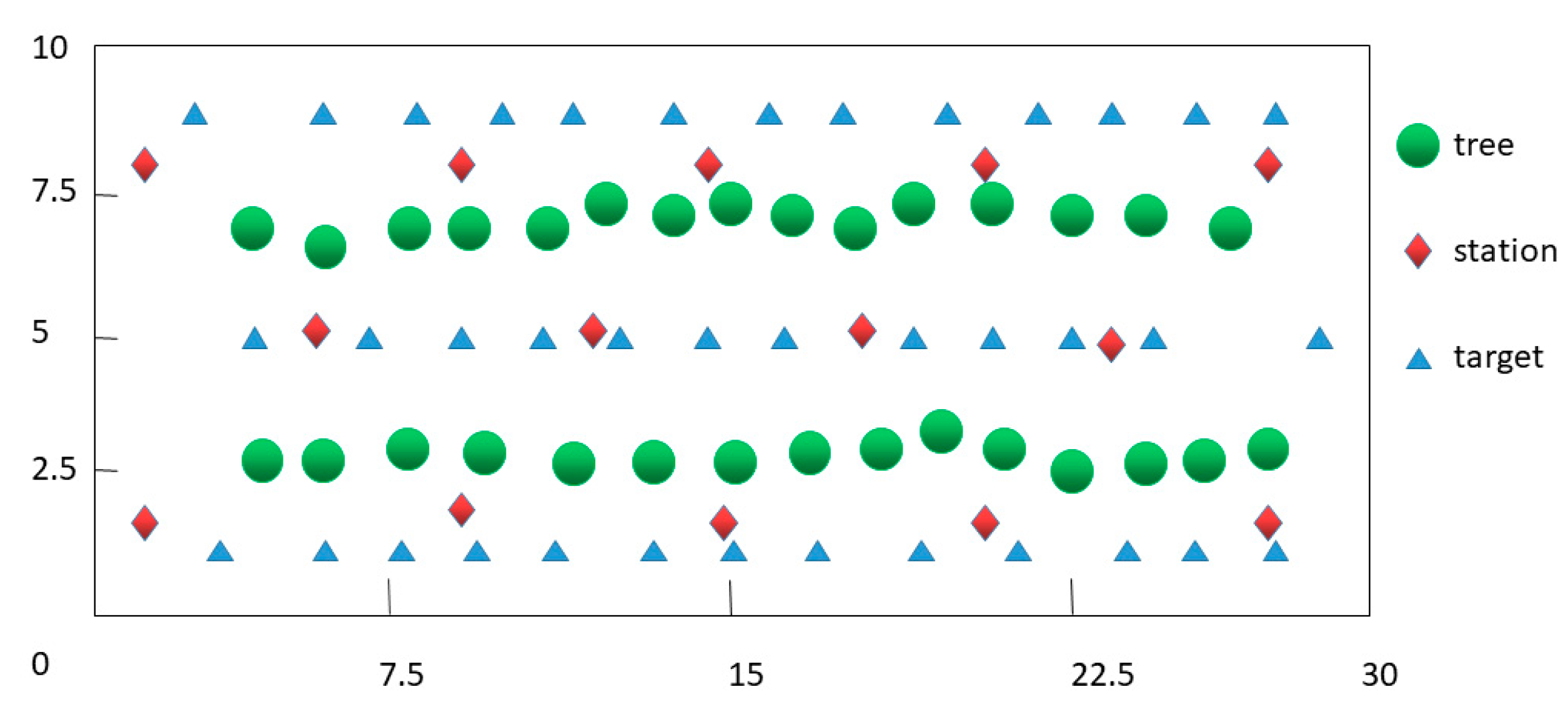
2.2.2. Measurement of Wind Speed and Air Volume

Fourteen monitoring sites were set up before and after the windbreak. In front of the forest, we set up sites at 3 H and 0.5 H, where H represents the average tree height of the sample site, in meters. The other monitoring sites were set up behind the forest. Wind speed and wind direction collection points were set up at 3, 6, and 9 m from the ground for each monitoring site. Each wind speed collection point monitored the instantaneous wind speed and wind direction simultaneously for more than 1 h. Wind speed was measured on the windward and leeward sides of the windbreak using an anemometer (YGC-FS) and wind direction meter (YGC-FX). Instrument parameters are shown in Table 2. Each measurement point consisted of a wind vane, light electric cup anemometers, and a wind speed alarm. These components were connected using data cables. During the measurement, all sensors were fixed to a high mast as needed. The data logger automatically recorded instantaneous wind speed and direction signals from the anemometer and wind direction meter every minute. The actual situation is shown in Figure 2 and Figure 3.

2.2.3. Calculation of Air Permeability Coefficient

The anemometer was set at 3, 6, and 9 m from the ground at the forest edge on the leeward side of the forest belt, and the wind speed was simultaneously measured at three heights v1’, v2’, and v3’; at 3 H on the windward side of the forest belt (representing the wind speed in the open field), the anemometer was also set at 3, 6, and 9 m from the ground and wind measurements at the three heights were also carried out simultaneously as v1, v2, and v3. The wind permeability coefficient was calculated [25] as:
α 0 % = v 1 + v 2 + v 3 v 1 + v 2 + v 3   ×   100 %

2.2.4. Calculation of Absolute Error, Relative Error, and RMSE

The following calculations were used:
Δ = r 1 r 2  
E = r 1 r 2 r 2 × 100 %  
RMSE = i = 1 n r 1 r 2 2 n
where Δ is the absolute error (m/s), E is the relative error (%), and RMSE is the root mean square error, m/s; r1 is the calculation result of each model; r2 is the actual measurement result of the sample site.

2.2.5. Calculation of Porosity

Current porosity measurement methods include visual inspection, square grid view frame method, probability estimation method, mathematical modeling method, and the use of the digital image analysis software Image-Pro Plus [26]. Combining a digital camera and the image processing software Photoshop [27] is the most common method for porosity determination in windbreak forest stands. However, these methods provide forest strip porosity with a crude approach, in which the conversion of color images into grayscale images for forest strip branches and pore segmentation is achieved by the naked eye. The solid areas of trees and pores are identified with a complicated and slow operation process, with low efficiency, which cannot avoid the interference of human factors. Additionally, measurement accuracy is greatly affected by wind speed and direction at the time of filming; therefore, it is not suitable for forest strip structure research. In this paper, we scanned the entire sample plot using TLS on the vertical line of the forest strip to determine the permeability coefficient. The spliced sample point cloud was input into the CloudCompare software and cropped to obtain a tree point cloud, which was modeled using the accurate and detailed quantitative structure model (AdQSM). Porosity was measured using the transparent diaphragm check method as follows:
β % = S 0 S × 100 %
where   S 0   is the light-transmitting void area, and S is the measurement range area.

2.3. Point Cloud Data Processing

2.3.1. Acquisition of TLS Data

We used a FARO Focus 3D X330 scanner to scan the sample plots and obtain their point cloud data. The FARO Focus 3D X330 is a high-speed 3D laser scanner with an extremely long measuring distance that allows the measurement of large, difficult-to-access woodlands at a distance in fewer scans, greatly increasing the speed of measurement. The specific parameters are presented in Table 3.
A total of 14 scanning stations were set up in and around the center of the sample plot. The sample plot settings, targets, and station locations are shown in Figure 4.
Each TLS was placed in turn at different locations and 3 m from the target tree. After the TLS scanning procedure was finished, each scan from a different angle was integrated into a single coordinate system by using a registration process to acquire full coverage scanning data from the objective trees. The first scan was placed at the center of each plot, and the rest were distributed along the periphery of each plot; the duration of each scan was 5 min. The device provides a 300° × 360° field-of-view acquisition, enabling optimal scanning performance of high-resolution scans up to 330 m and generates 555 M pts/scan. The TLS has a maximum distance range of 300 m (for most surfaces), a scanning speed of 1 M pts/s, and the collected TLS data had an average point density of 1,362,692 pts/m2. A field-instant method was used to calibrate the laser scanner. In practice, targets were placed within 1 m of the preset locations to minimize the shading effect between trees and to facilitate better data acquisition. The scan results are shown in Figure 5.

2.3.2. Filtering of Ground and Off-Ground Points

All the collected TLS data were preprocessed following the same procedure, including transformation, clipping, denoising, filtering, and normalization. After the pre-processing phase, the point clouds were extracted and imported into the CloudCompare software V.2.10. where the cloth simulation filter algorithm, as a third-party plug-in, was applied to separate and extract the ground from the off-ground points. In the general parameter setting tab of the surface base filter, the relief terrain option was chosen because of the slightly inclined plane in the plots. For calibration, cloth resolution was set to 1.1; for maximum iterations, we used 500.

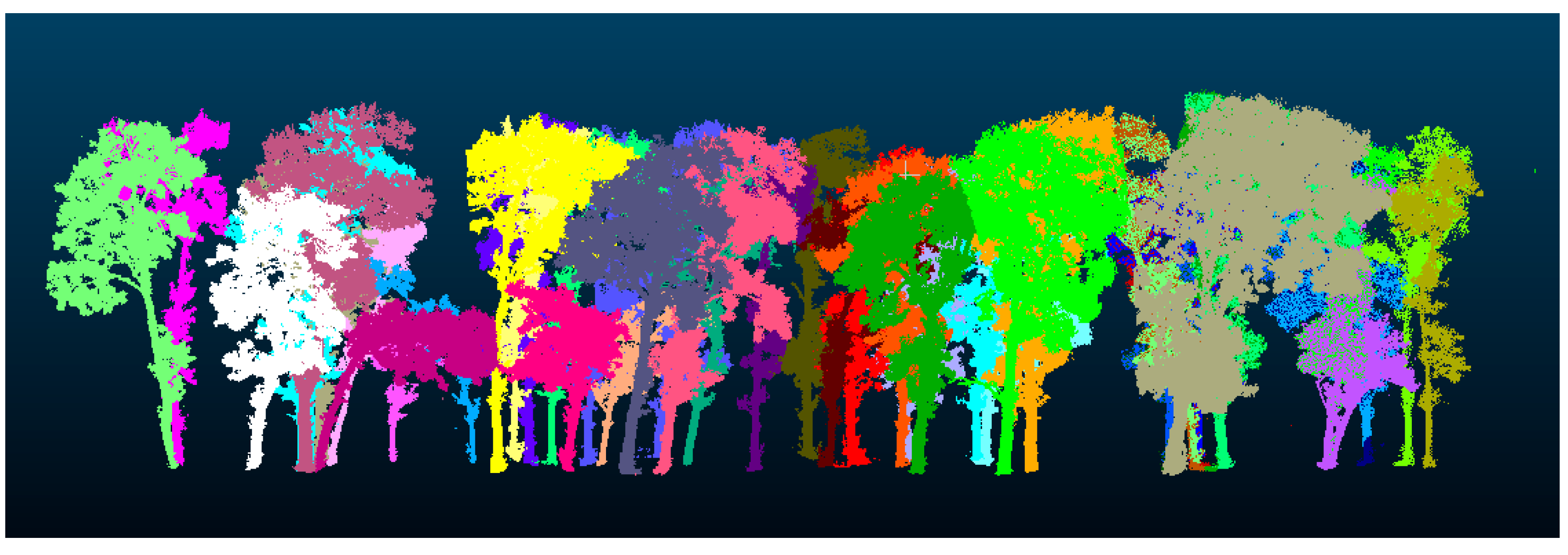
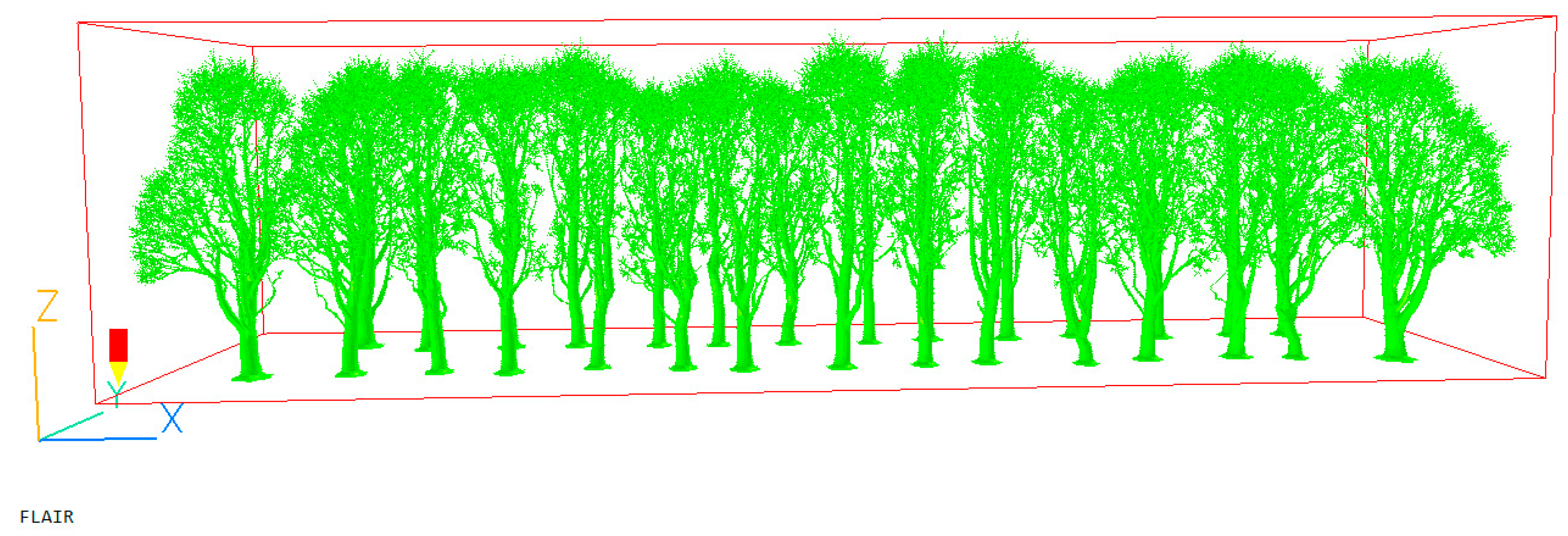
2.3.3. Three-Dimensional Structural Reconstruction of the Windbreak Forest Belt

The 3D model of the windbreak forest sample site was modeled using AdQSM. AdQSM can read the input point clouds in approximately 4–8 s and quickly model a single tree with a realistic appearance in terms of trunk and crown dimensions. A single tree is represented as a closed, fully convex polyhedron, and the single tree model reconstructed by AdQSM can estimate parameters such as volume, tree height, diameter at breast height, total branch count, live crown height, and crown size, allowing monitoring of natural progressive changes in biomass and sudden changes caused by storm damage, crop harvesting, fire, or pests and diseases. The 3D tree reconstruction by AdQSM provides an opportunity for a realistic representation of the windbreak forest scenario. Its accuracy and realism can be applied to point cloud modeling. This information is essential for developing effective windbreak forest management strategies. In this study, we collected measurements of the diameter at breast height, height, and crown width of single trees before modeling, and related data after modeling was completed, and performed error analysis. Figure 6 shows the collected point cloud data and the results after modeling.

2.4. Wind Field Simulation

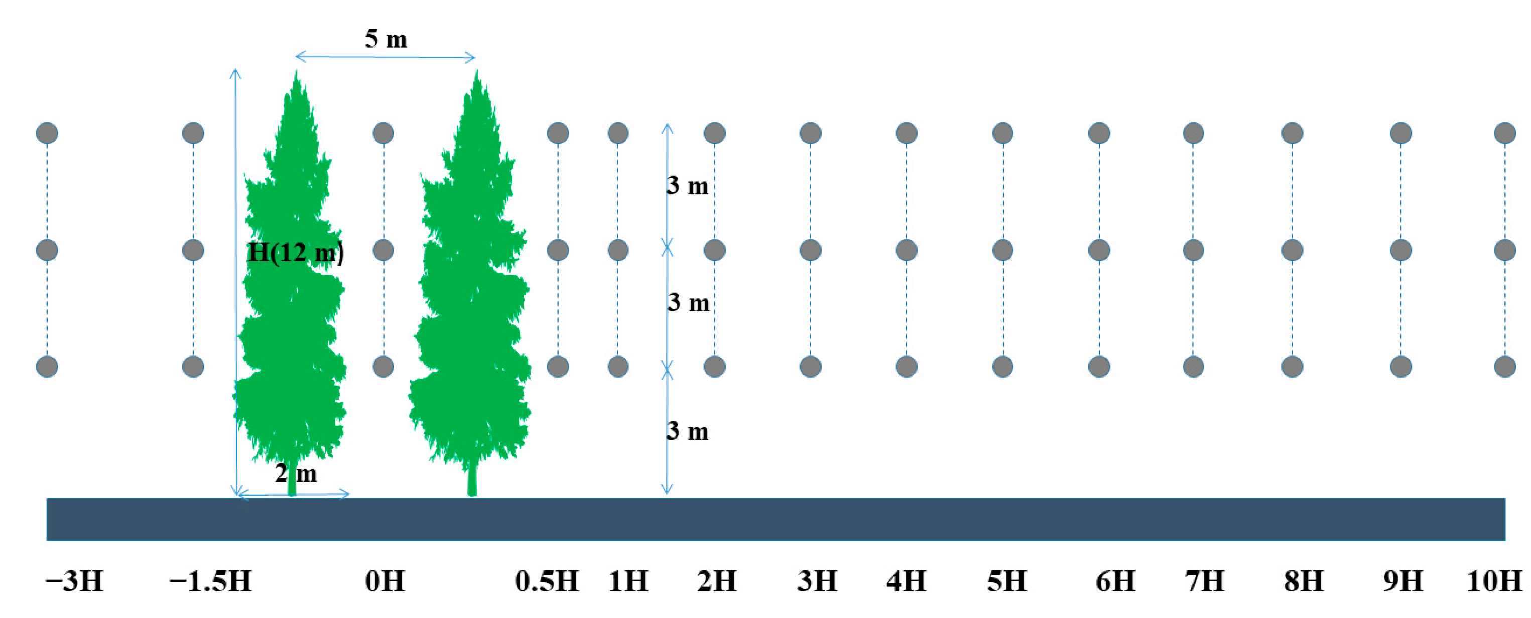
2.4.1. Geometric Model and Computational Domain

In this section, wind speed was evaluated using a 3D model of the alternative windbreak forest. The model principle and placement of the windbreak forest are shown in Figure 7. The windbreak forest had 30 trees with an average height of 12 m, divided into two rows of 15 trees each, with a spacing of 2 m between the trees in the same row and a spacing of 5 m between the front and back rows. The inflow boundary was 8 H from the nearest trees; the spacing between the left boundary and the left windbreak forest was 6 H; the spacing between the top boundary and the top of the tallest trees was 5 H; and the outflow boundary and the nearest spacing between the outflow boundary and the nearest trees was 12 H, which satisfied the CFD criterion and was large enough to avoid backflow pressure.

2.4.2. Boundary Conditions

According to the boundary conditions, the calculation domain was divided into inlet and outlet.
The wind speed 9 m above the ground in different directions was obtained by averaging the cumulative wind speeds at different frequencies in August at the sample site in Zhangbei. This value was set as the initial velocity in the simulation and was set to 7 m/s.
To consider the influence of the crop surface on the flow velocity, the exponential power-law flow velocity was used as the inlet flow velocity boundary condition, using the following equation:
U z = U s z z s α
I z = 0.1 × z z G α 0.05
k z = I z × U z 2
ε z = C μ 0.5 × k z × U s × α z s × z z s α 1
where Z G is the atmospheric boundary layer height (determined by the local topography), Z S is the reference height, Z is the calculation point height, C μ is a constant (0.09), U S is the average wind speed at the reference height, U Z is the wind speed calculation point, and α is the ground roughness coefficient. Since the study area was located in the countryside, the ground roughness coefficient was set to 0.16.
In this study, the inlet was defined as the velocity inlet boundary, the outlet was the specified constant pressure, the upper boundary and left and right boundaries were defined as symmetric boundaries, and the ground and windbreak forest boundaries were determined by the wall function method.

2.4.3. Numerical Model

In this study, PHOENICS (Parabolic Hyperbolic Or Elliptic Numerical Integration Code Series) software [28] was used to build a model to simulate the wind field environment of a windbreak forest. The PHOENICS software is a general CFD software for simulating heat transfer, flow [29], chemical reactions, and combustion [30] processes and can be used to solve steady-state flow turbulence models in three-dimensional space.
The basic control equation for PHOENICS simulations is the Navier–Stokes (N-S) equation [31], expressed as follows:
ρ ϕ t + d i v ρ u ϕ Γ ϕ ϕ = S ϕ
where ϕ is the variable to be found, such as the temperature and velocity; ρ is the density, kg/ m 3 ; u is the velocity in each direction (m/s); Γ is the convective term; S ϕ is the source term; and t is the time (s).
We chose the improved RNG   k e p s i l o n model, which is a turbulence model commonly used in engineering calculations. The method is low-cost, highly applicable, easy to use, and fast to compute, and has been widely used in the numerical simulation of outdoor wind field environments.
Currently, some scholars use the standard RNG k-epsilon model to calculate ambient air temperature and wind speed [32,33], Although the standard k ε model has been widely used, the improved RNG k ε model yields higher accuracy by modifying the turbulent viscosity, considering the rotating mean flow, and increasing the mainstream strain rate reflected in the epsilon equation. The momentum and mass conservation equations can be expressed as follows:
U i t + U j U i x j = 1 ρ P * x i + v 2 U i x j x j x j u i u j ¯ + 1 ρ F t r e e , i
U j x j = 0
where x i , U i ,   P * are the parameters of the Cartesian coordinate system (i = 1,2,3), respectively; ith denotes the average velocity air volume and the deviation of pressure from the reference value; ρ and υ are the air density and kinematic viscosity, respectively; and U i denotes the fluctuation of the average velocity component from i . The Reynolds stress in Equation (9) is parameterized as follows:
u i u j ¯ = K m U i U j + U j U i 2 3 δ i j k
where K m and k are the turbulent diffusion coefficient and turbulent kinetic energy of momentum, respectively. The turbulent diffusion coefficient of momentum is determined by the turbulent kinetic energy and its turbulent kinetic energy dissipation rate ε , as follows:
K m = C μ k 2 ε
where C μ is the empirical constant (0.09) for the improved RNG k ε turbulence closure scheme.
The prediction equations for the turbulent kinetic energy and the improved RNG k ε turbulence closure format are:
k t + U j k x j = u i u j ¯ U i x j + x j K m σ k k x j ε + F t r e e , k
ε t + U j ε x j = C ε 1 ε k u i u j ¯ U i x j + x j K m σ k k x j C ε 2 ε 2 k R s + F t r e e , k
where R s is the given strain rate, expressed as:
R s = C μ η 3 1 η / η 0 ε 3 1 + β 0 η 3 k
η = k ε U i x j + U j x i U i x j 1 / 2
where C ε 1 , C ε 2 , σ k , σ ε and η 0 are empirical constants, as follows:
( C ε 1 , C ε 2 , σ k , σ ε , η 0 ) = ( 1.42 ,   1.68 ,   0.7179 ,   0.7179 ,   4.377 ,   0.012 ) .

3. Results and Analysis

3.1. Model Accuracy Validation

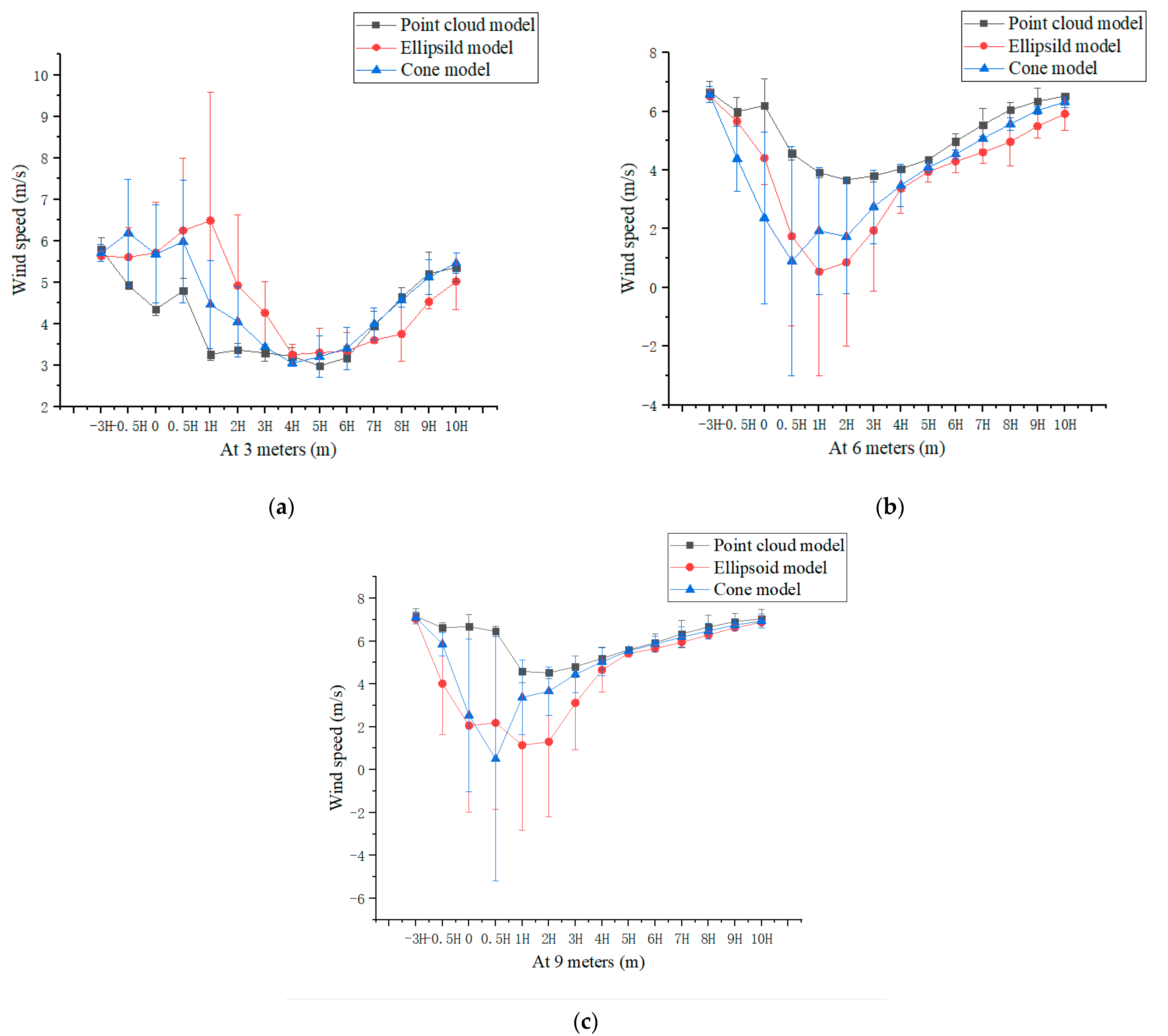
3.1.1. Comparison of Simulated and True Values of Wind Speed

To analyze and test the accuracy of the three models, we compared the accuracy of the measured data of the sample site with the simulation results of the three different models. The same locations and heights were selected for the pre-forest, in-forest, and post-forest areas.
Finally, we obtained the wind speed data from 14 different locations, and each model was divided into three heights. The absolute error, relative error, and root mean square error of the three simulations were used to quantify the differences between the simulations and were calculated as follows:
From the calculation results in Table 4, the accuracy of the point cloud model is higher than that of the other two models at most positions. The maximum relative error was 91.9% for the 0.5 H conical canopy at 9-m height and the minimum was 0.1% for the 7 H ellipsoidal canopy at 3-m height; the root mean square errors were 0.272, 0.377, and 0.437 for the point cloud model at 3, 6, and 9-m heights, respectively; the RMSEs were 1.184, 1.635, and 2.272 for the ellipsoidal model at each height, respectively, and the RMSEs for the conical model at each height were 0.759, 1.600, 1.921. In most positions, the error of the simulation results of the point cloud model was the smallest, and the errors of the simulation results of the other models varied according to the position and height.
Note: Yellow and green markers are the maximum and minimum values, respectively.
The representative wind speed at 3-m height was used as the reference value for comparison and validation. From the wind speed trends and absolute errors in Figure 8a, we calculated the average deviation of the point cloud model to be 0.128 m/s, the average deviation of the ellipsoidal model to be 0.654 m/s, and the average error of the conical model to be 0.56 m/s among the 14 positions at the same height in the whole sample site. This was significantly higher than that of the other two models, and the wind speed error was largest at 3 H in front of the forest and 4 H behind the forest. Among them, the ellipsoidal model had the largest error of up to 3.088 m/s.

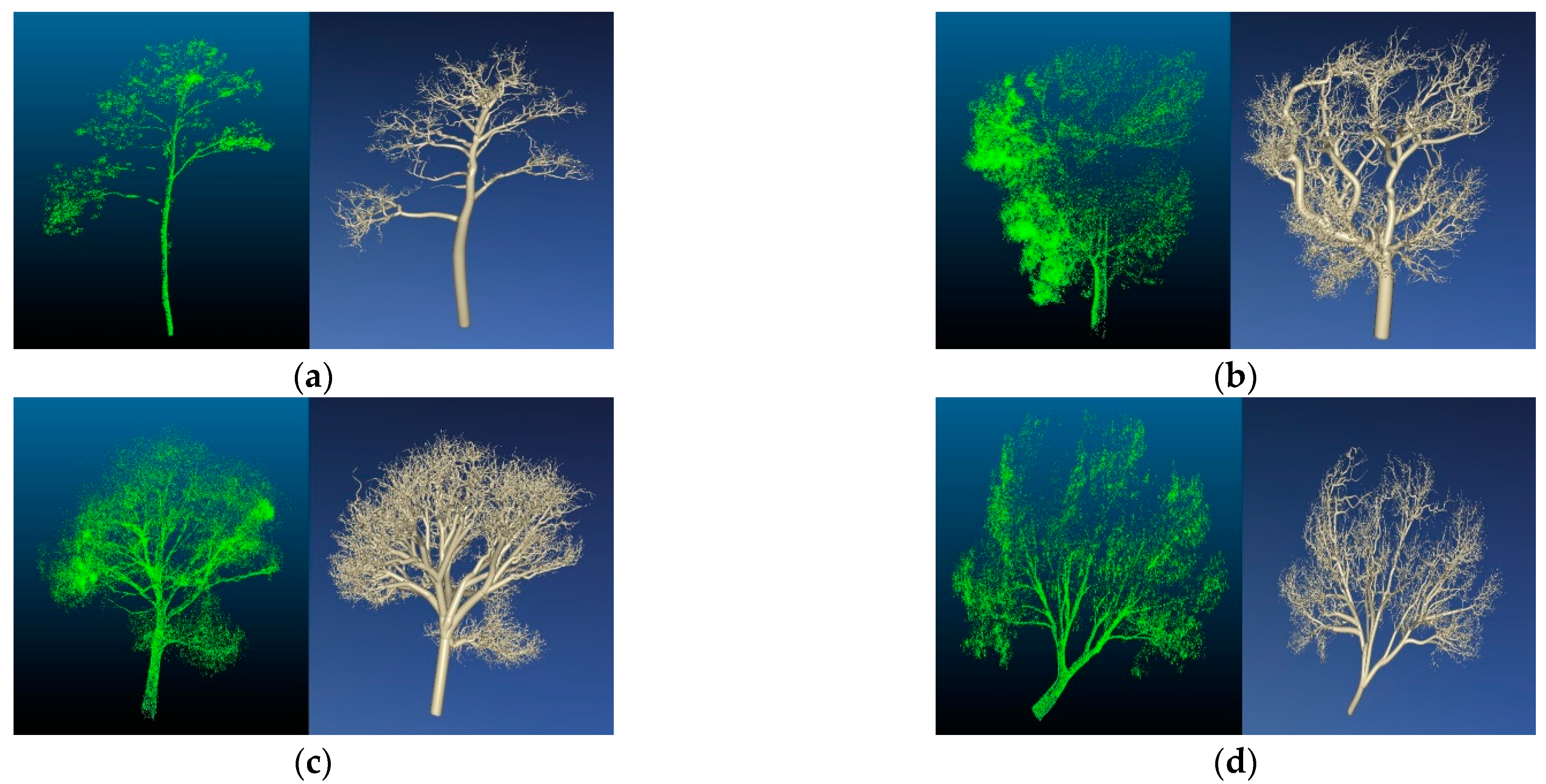
3.1.2. Comparison of Model Structure and True Values of Individual Trees in Windbreak Forests

During the sample site inventory, we manually measured the diameter at breast height, height, and crown width of each tree. The AdQSM automatically calculated parameters such as the diameter at breast height, height, and crown width for the point cloud model. The results of the comparison are presented in Table 5.
From the calculation results in Table 5, it is generally seen that the modeling effect is more accurate when using TLS to collect point cloud data of windbreak forests and AdQSM for individual tree modeling. The absolute and relative errors were slightly larger because the crown width error was measured manually using a tape measure, and for five of the trees, the modeled crown width error was large, with a maximum error of 9.6%; however, for the diameter at breast height and tree height, the modeled results were very close to the true values.

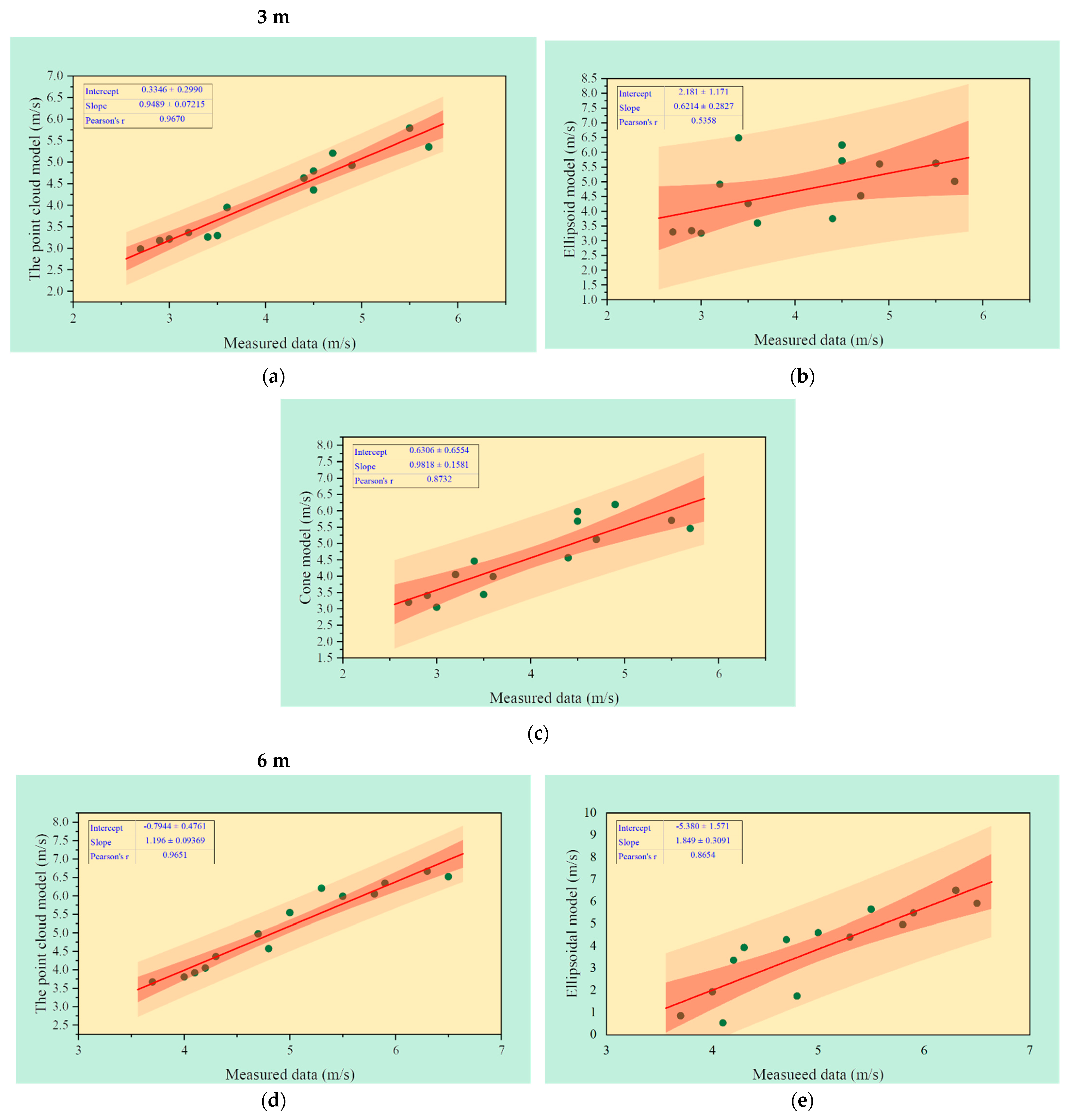
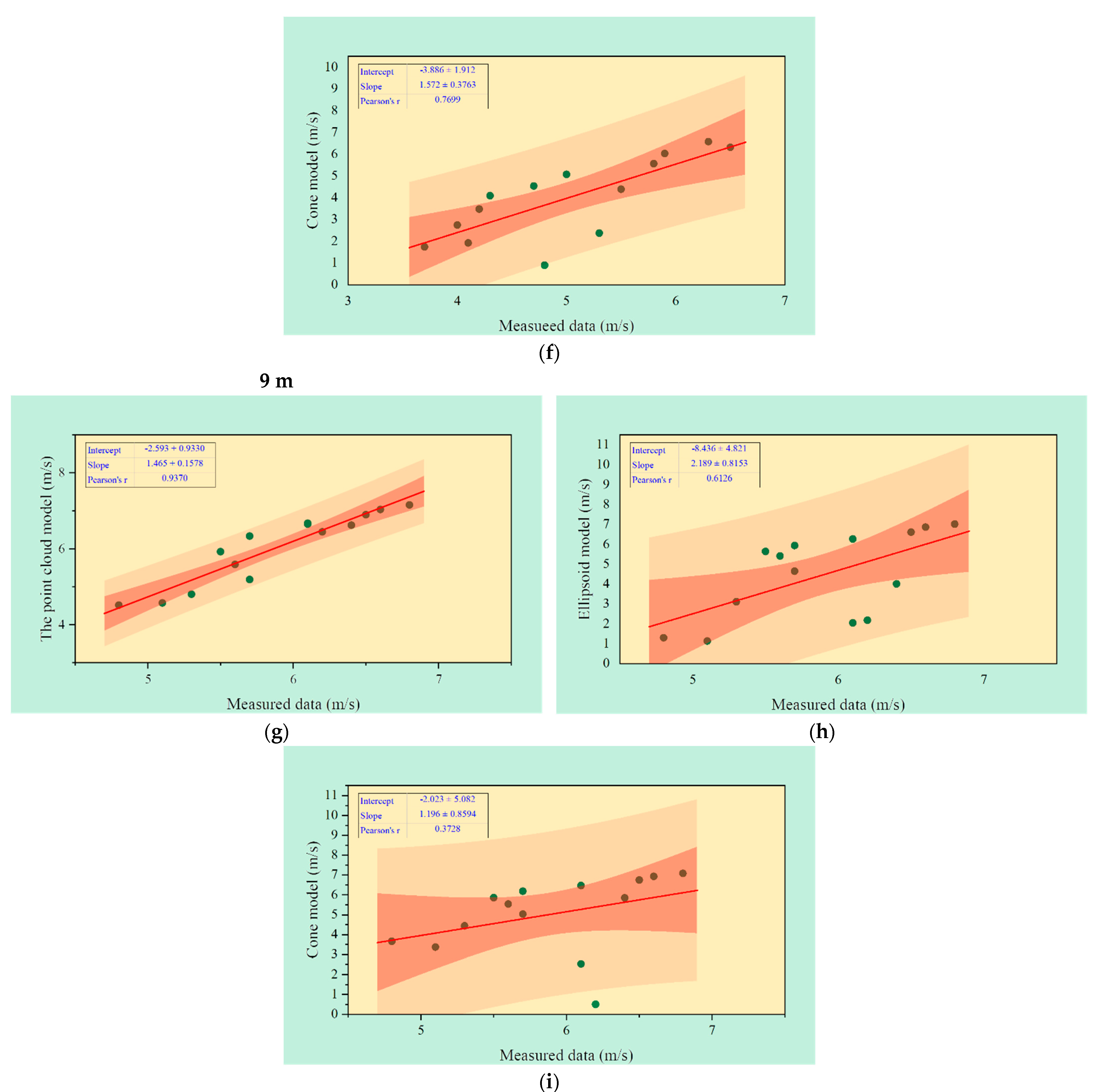
3.2. Reliability Analysis of Actual Wind Speed Measurements and Each Simulation Result

From the comparison results of the simulated and measured data of different models at different heights, the correlation coefficients of the point cloud models at three heights from 3, 6, and 9 m were 0.967, 0.965, and 0.937, respectively. A decreasing trend was observed with increasing height. The correlation coefficients of the ellipsoidal model were 0.5358, 0.8654, and 0.6126, respectively, indicating that this model had a higher simulation accuracy at 6-m height. The correlation coefficients of the conical model were 0.8732, 0.7699, and 0.3728, respectively, indicating that the accuracy of this model gradually decreased with increasing height. The simulation results showed that the simulated experimental results of the point cloud model were in good agreement with the test data, in line with the wind speed variation law, and with the highest fitting accuracy. Figure 9 shows the correlation analysis of the three models at different heights.

3.3. Velocity Analysis of Different Positions

To verify the reproducibility and accuracy of the TLS model input CFD, the simulation results were analyzed together with two other canopy models of different structure types, and the resultant data were compared to observe the wind velocity flow field patterns at different locations of the sample site. As shown in Figure 10, the wind velocity in the Y-direction before the airflow reached the windward side of the canopy is the entrance wind velocity. At the same height, the wind velocity after the airflow has passed through the three canopy types showed a step change, owing to the obstructing effects of the forest. In the canopy model using real modeling of point cloud data, the area of the region of low wind velocity was the largest because of low porosity, followed by the ellipsoidal canopy; the conical canopy had the smallest area.
The greatest reduction in wind speed was observed in the 0.5–1 H region behind the three modeled forest strips at 3-m height. The modeling of a windproof forest established by point clouds reduced the wind speed from 7 m/s to 2.984 m/s, or by 57.4% [34]. The wind speed distribution in the region of 5–10 H ranged from 3.174 to 5.724 m/s, with a reduction of approximately 18.2 to 54.7%. When the horizontal distance was greater than 10 H, the wind speed value returned to the level of the open-field wind speed value, that is, the windbreak forest belt loses its protective function. The aerodynamic effect of wind speed reduction in a certain area of the forest belt was fully reflected [35]. When the wind passes through the canopy and dry layer of the forest belt, the airflow is divided into two parts, and the airflow above the back of the forest sinks to meet the part of airflow passing through the forest to form vortices; thus, the back of the forest belt has a certain wind reduction area range, so all observation points behind the forest belt have different degrees of wind protection benefits. In the back of the forest, owing to the upper layer of airflow, the wind protection effectiveness was gradually reduced to only 18.2% at 10 H in front of the forest. Therefore, the wind protection effectiveness of windbreak forest strips varied at different horizontal distances. Considering 5 H after the forest belt of the different models as the control, the wind protection effectiveness of each observation point after the forest belt was different, and the wind speed reduction was 57.4% for the point cloud model, 55.7% for the ellipsoidal model, and 56.4% for the conical model.
It is not difficult to find that the windbreak wind-blocking effect is greatest at a height of 3 m because of the greatest width of the canopy here; the smaller the porosity at the same time, the more pronounced the blocking effect. The maximum difference between the maximum and minimum values of velocity was 3.72 m/s inside the real canopy sample established by TLS data, while the velocity difference was only 2.21 m/s at other locations within the forest because the airflow can pass through more easily inside the sparse canopy. From (a) and (g) in Figure 10, it can be seen that there is an increase in airflow velocity at the lower and higher parts of the stand, which is because of the blocked airflow from above and below the canopy, causing an increase in wind speed. Thus, the TLS-modeled 3D forest stand better reflected the velocity field distribution, pressure field distribution, and kinetic energy intensity variations.

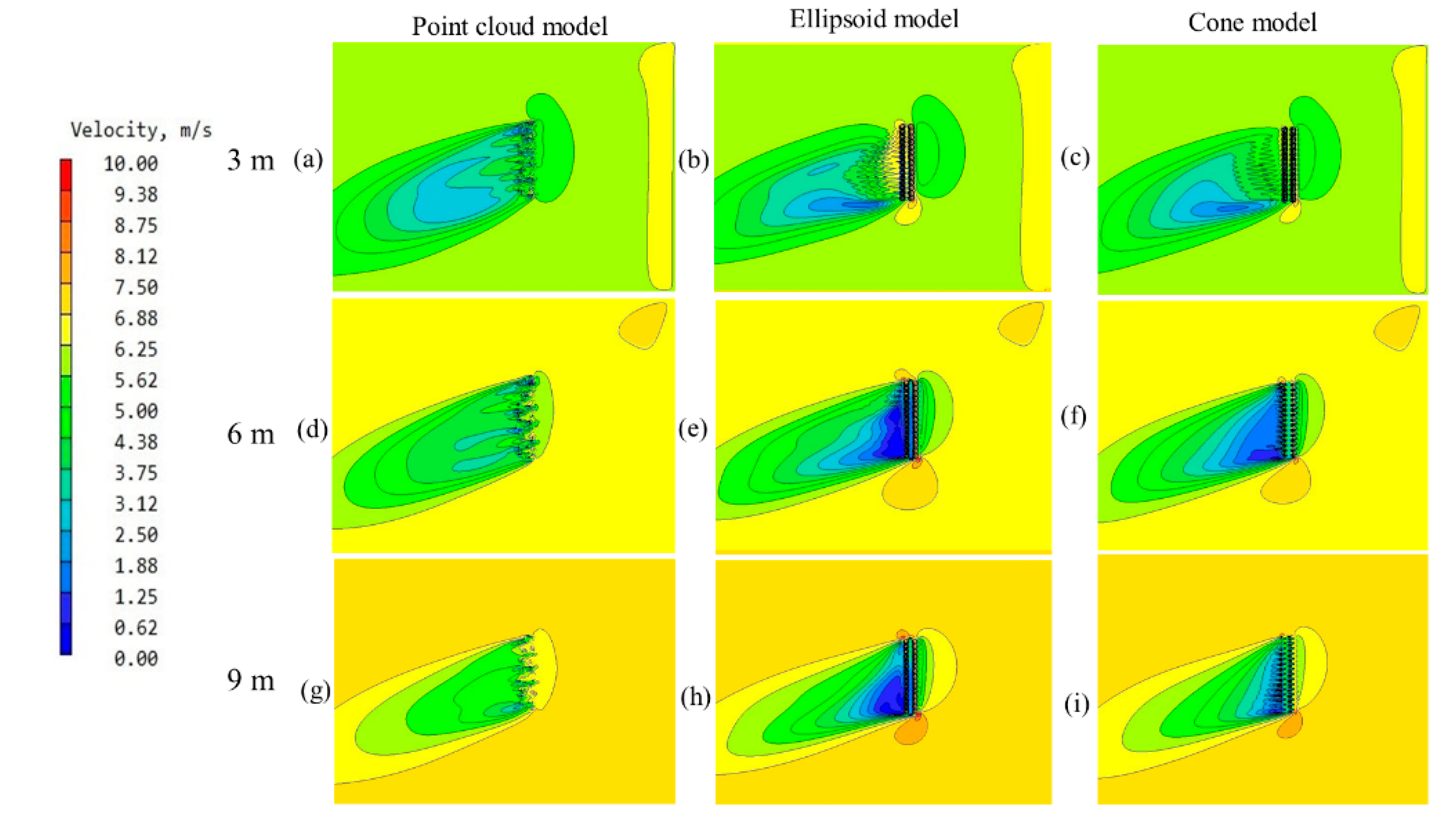
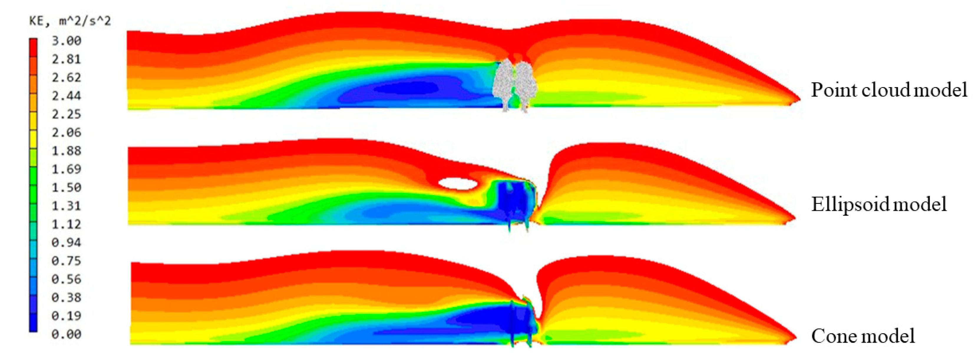
3.4. Kinetic Energy Cloud Diagram for Three Models

To reveal the effects of the three windbreak forest structures on wind speed more clearly, we selected a vertical surface at the same location in the middle of the study area to determine the vertical turbulence degree distribution as an inverse view of the simulated wind speed of each model (Figure 11). The kinetic energy intensity clouds show that in the real model established by the TLS data, the kinetic energy was mainly gathered at the back of the forest. The kinetic energy generated by all three stand models was concentrated at 0–5 H after the windbreak, and the kinetic energy formed around the canopy of the real model established by the point cloud data was significantly lower than that of the remaining two canopies, it means it has the best blocking effect on the airflow. The general rule of kinetic energy change for all three models started from 5 H, and the further away from the forest stand, the higher the kinetic energy; that is, a kinetic energy reduction zone is formed in the range from 0 to 5 H. Therefore, in the middle of the stand, the area of the post-forest low kinetic energy zone was the largest because the point cloud model had the smallest porosity, which made it difficult for the airflow to pass through, causing low wind speed.

4. Discussion

In this study, we used TLS to scan a double-row farmland windbreak forest and modeled the point cloud data using AdQSM. The accuracy of the point cloud model and the ellipsoidal and conical models commonly used in related studies were verified using the CFD software PHOENICS, which was used to conduct wind field simulations of the experimental sample sites. Herein, we discuss the most important findings of this study.

4.1. AdQSM Applicability Assessment

4.1.1. Restoring the Structural Aspects of Trees

The AdQSM method based on the TLS point cloud reconstruction of trees is important for estimating the structure factor of an individual tree. In this study, the accuracy of tree structure measurements in windbreak forests with TLS was very high, especially for tree height and diameter at breast height, with an accuracy of over 95%. The tree crown had the worst extraction accuracy, with an average of 92%. This was because the point cloud of the upper part of the canopy was missing because of partial shading between the trees at the top of the tree during modeling, resulting in a partially incomplete final model. In this study, based on the results of Kumazaki and Kunii [33], five single trees were randomly selected from the TLS-scanned experimental site, and the modeling results were compared with the real results using AdQSM. For these five random samples, the absolute errors of three factors (diameter at breast height, height, and crown width) were less than 5 mm, the relative errors of diameter at breast height and height were less than 2%, and the relative errors of crown width were larger (approximately 8%) because of the shading between trees. Although the five trees were randomly sampled at different locations in the experimental area, the differences between the breast diameter and tree height estimated by AdQSM and the true values were small.

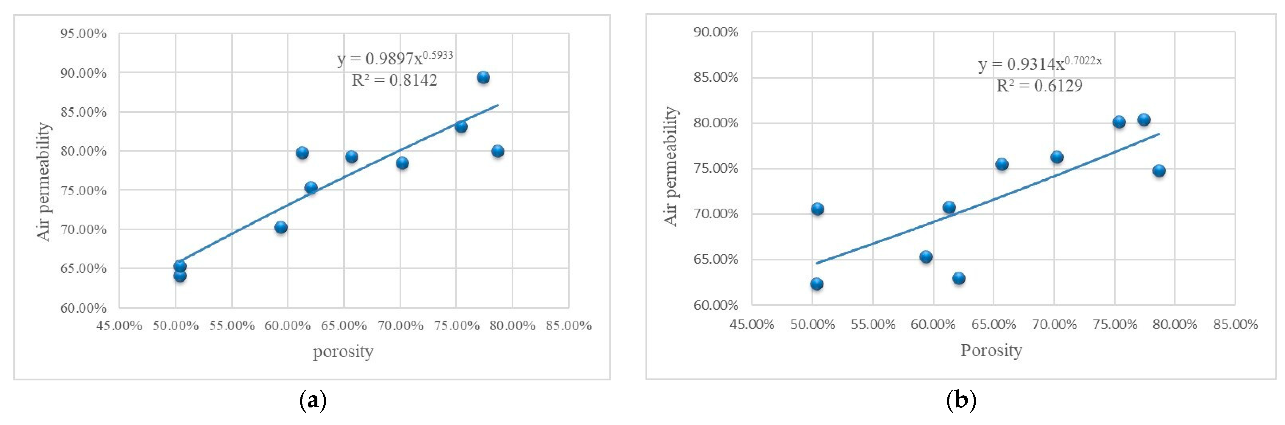
4.1.2. Fitting of Wind Permeability Coefficient and Porosity

We fitted the measured wind permeability coefficients at 10 different locations in the study area with the porosity values calculated using two different methods: the AdQSM modeling method and the digital image analysis method (Figure 12). A one-dimensional exponential regression analysis method was applied, with porosity (β) as the independent variable and air permeability coefficient ( α 0 ) as the dependent variable. The correlation coefficient derived from the AdQSM modeling method (0.8142) was higher than that derived from the digital image analysis method (0.6129). The approximate conversion relationship between the porosity and wind permeability coefficient was obtained according to Donghui et al. [36]. For a two-row forest belt, α 0 = β 0.6 therefore, the windbreak forest calculated by the AdQSM modeling method is more accurate, and the modeling using AdQSM in this study met the requirements of the windbreak effect simulation. This indicates that the porosity of the windbreak forest determined using TLS is more accurate and can also be used for the determination of windbreak forest porosity.

4.2. Accuracy Analysis of Measured Wind Field Data and Simulated Wind Field Data

To compare the magnitude of the effect of different types of canopy structures on the wind protection effect of windbreaks, we conducted wind field simulations under the same conditions of plant spacing, canopy width, and mean height for all three models; however, the wind speed results obtained differed significantly depending on the canopy structure. The main reason for this is that porosity is one of the most important structural parameters of windbreaks, which determines their efficiency in reducing wind speed and shading areas. In all windbreak studies, the best optical porosity values for the most effective windbreaks ranged from 20 to 40%. In this study, the porosity of the point cloud model windbreak forest was approximately 34%, which is within the range reported by Wu et al. and others [37,38]. In contrast, the calculated porosity was approximately 51% for the ellipsoidal model windbreak and 67% for the conical model windbreak, which was out of range. Thus, the findings indicate that windbreaks with different porosities have significantly different degrees of wind reduction in wind simulations. The point cloud model showed a mean wind speed reduction of 58% 5 H behind the stand, and the same position showed a mean wind speed reduction of 49% for elliptical canopies and 43% for conical canopies, which is similar to the results of Torita and Satou and Bitog et al. in the relationship between windbreak structure and wind reduction [39]. Different canopy structures determine different porosities, and for double-row windbreaks, the second row of trees enhances resistance and improves the overall wind reduction efficacy of the windbreak. With a certain spacing between the front and rear rows, the effective density of the entire windbreak increases because of the blocking effect of the second row when the wind passes through the first sparse and then dense stand. Unlike the study by Gross, the difference in porosity leading to the difference in the internal structure of windbreaks varied greatly for the results of wind and sand fixation.
From the simulation results in Section 3.1, it can be observed that the greatest reduction in wind speed is observed when the airflow passes through the windbreak, that is, in the 0.5–1 H region behind the forest zone, for all three models. However, owing to the difference in canopy structure, for the conical canopy with the largest porosity, the porosity increases as the height continues to increase, resulting in a smaller area and a faster rate of reduction in the low wind speed region 0–8 H behind the forest, which is the same as the results of Hagen et al. and Torshizi et al. In addition, the point cloud model can better simulate the wind separation recirculation process and its size and location with porosity, leading to a critical porosity of separation that is consistent with the observed values. The simulated location of the maximum wind speed reduction, variation of the maximum wind speed with porosity, rate of leeward wind speed recovery, and simulated aerodynamic properties agree with the field observations. From the aspect of kinetic energy, for the same wind speed and direction, in the point cloud model with the lowest porosity, the blue area of the low-speed region is larger than that of the other two models, which indicates that when the wind passes through the forest belt, owing to the small porosity of the point cloud model, the wind pass through normally. Rather, part of the airflow was obstructed by the forest belt and lifted to the top of the forest belt. After crossing the forest belt, this part of the airflow forms a high wind speed region, whereas, behind the forest, the airflow above the sinks meets with the part of the airflow passing through the forest belt to form vortices to form a low wind speed region. The wind speed recovers rapidly as it moves away from the forest belt until it approaches the initial wind speed, which is similar to the conclusions of Mayaud et al. (2016) that the wind speeds return to equilibrium in an exponential form after traversing the forest [40].
In summary, the point cloud model was able to accurately restore the structure of the trees in the experimental sample site, where the simulations yielded results closest to the true values of wind speed in the sample site at most locations. This is unmatched by the other structural models.

4.3. Study Limitations

Owing to resource limitations, we selected only one local tree species for the simulation. The simulation results may vary depending on the experimental area. Moreover, there are several types of windbreak configuration structures, and double-row windbreaks are only one of them. The windbreak effects of different windbreak configurations vary significantly, and the results of this study can provide a reference for future windbreak-related studies. In addition, there are various CFD simulation tools, and different computational fluid dynamics simulation software may yield different results for this study and should be explored in future studies. Moreover, the wind field meter used in this study is a three-cup wind field meter, which can only achieve a single point measurement, and the height of the observation is determined by the height of the stand; therefore, there are inevitable errors in the measurement. If a wind measurement LIDAR system is used to measure the wind field information of the study area as a whole, the research results may be more accurate. Due to the forest canopy, it is difficult for TLS to obtain the upper forest canopy point cloud, which leads to less accurate modeling results. For the acquisition of forest canopy point cloud data in the future, advanced unmanned aerial vehicles should be combined with both types of point cloud data for modeling to carry out accurate studies of windbreak effects in windbreak forests. Therefore, accurate modeling of individual trees remains the focus of future research.

5. Conclusions

In this study, we used TLS and AdQSM to model the effects of a windbreak forest on agricultural land and PHOENICS to simulate the wind field and analyze the effects of canopy models with three different porosities on the wind environment. The results showed that modeling TLS data with AdQSMA can extract forest structure parameters, demonstrating its usefulness in windbreak forest-related studies. Compared with traditional approaches, this method has the advantages of automation, accuracy, speed, and efficiency. We also showed that different canopy types had different effects on the windbreak effect. Among them, the simulation results of the point cloud model were the most accurate for determining the maximum wind speed reduction, variation of the maximum wind speed with porosity, and recovery rate of the leeward wind speed. We analyzed the effects of different windbreak model structures on wind speed, reflecting the advantages of TLS applied in windbreak forest engineering. Only the accurate modeling of windbreaks can provide an accurate assessment of the wind effect of windbreaks. The research method used in this study will provide a reference for future scientific research on windbreaks. Finally, the superiority of TLS in the extraction of structural factors and other applications of windbreaks indicates a promising direction for future research related to the simulation of windbreak effects.

Author Contributions

Conceptualization, L.A. and J.W.; methodology, L.A.; software, L.A. and Y.W.; validation, L.A., N.X., Y.W., J.Y. and H.L.; formal analysis, Y.W., J.Y. and H.L.; investigation, L.A., Y.W., J.Y., H.L., and N.X.; resources, J.W.; data curation, L.A.; writing—original draft preparation, L.A.; writing—review and editing, L.A. and J.W.; visualization, L.A.; supervision, J.W.; project administration, L.A.; funding acquisition, J.W. All authors have read and agreed to the published version of the manuscript.

Funding

This research was funded by the National Natural Science Foundation of China (Nos.31870713, 42171329, and 42071342) and the Natural Science Foundation of Beijing, China (8222069, 8222052).

Acknowledgments

We would like to thank Tao Zhang from the Forest Conservation Department of Beijing Forestry University and Shiyu Zhu from Wuhan University for helping us check the data.

Conflicts of Interest

The authors declare no conflict of interest.

References

  1. Chang, X.; Sun, L.; Yu, X.; Liu, Z.; Jia, G.; Wang, Y. Windbreak efficiency in controlling wind erosion and particulate matter concentrations from farmlands. Agric. Ecosyst. Environ. 2021, 308, 107269–107277. [Google Scholar] [CrossRef]
  2. Yang, Y.; YY-t Zhi, W.; Sun, G.; Cheng, F.u. Studies on Wind Break and Sand Fixation Effects of Farmland Shelterbelt in Bashang Area of Northern Hebei. J. Northwest For. Univ. 2020, 35, 167–172. [Google Scholar]
  3. Duryea, M.L.; Kampf, E.; Litell, R.C.; Rodriguez-Pedraz, C.D. Hurricanes and the Urban Forest: Ⅱ. Effects on Tropical and Subtropical Tree Species. Arboric. Urban For. 2007, 33, 98–112. [Google Scholar] [CrossRef]
  4. Meng, Z.; He, M.; Tao, Z.; Li, B.; Zhao, G.; Xiao, M. Three-Dimensional Numerical Modeling and Roof Deformation Analysis of Yuanjue Cave Based on Point Cloud Data. Adv. Civ. Eng. 2020, 2020, 8825015. [Google Scholar] [CrossRef]
  5. Koenig, K.; Höfle, B.; Hämmerle, M.; Jarmer, T.; Siegmann, B.; Lilienthal, H. Comparative classification analysis of post-harvest growth detection from terrestrial LiDAR point clouds in precision agriculture. ISPRS J. Photogramm. 2015, 104, 112–125. [Google Scholar] [CrossRef]
  6. Yun, T.; An, F.; Li, W.; Sun, Y.; Cao, L.; Xue, L. A novel approach for retrieving tree leaf area from ground-based LiDAR. Remote Sens. 2016, 8, 942. [Google Scholar] [CrossRef] [Green Version]
  7. Indirabai, I.; Nair, M.V.H.; Jaishanker, R.N.; Nidamanuri, R.R. Terrestrial laser scanner based 3D reconstruction of trees and retrieval of leaf area index in a forest environment. Ecol. Inform. 2019, 53, 100986–100996. [Google Scholar] [CrossRef]
  8. Saarela, S.; Wästlund, A.; Holmström, E.; Mensah, A.A.; Holm, S.; Nilsson, M. Mapping aboveground biomass and its prediction uncertainty using LiDAR and field data, accounting for tree-level allometric and LiDAR model errors. For. Ecosyst. 2020, 7, 43. [Google Scholar] [CrossRef]
  9. Takeda, T.; Oguma, H.; Sano, T.; Yone, Y.; Fujinuma, Y. Estimating the plant area density of a Japanese larch (Larix kaempferi Sarg.) plantation using a ground-based laser scanner. Agr. Forest Meteorol. 2008, 48, 428–438. [Google Scholar] [CrossRef]
  10. Wang, Y.; Wang, J.; Chang, S.; Sun, L.; An, L.; Chen, Y. Classification of street tree species using UAV tilt photogrammetry. Remote Sens. 2021, 13, 216. [Google Scholar] [CrossRef]
  11. Raumonen, P.; Kaasalainen, M.; Åkerblom, M.; Kaasalainen, S.; Kaartinen, H.; Vastaranta, M. Fast automatic precision tree models from terrestrial laser scanner data. Remote Sens. 2013, 5, 491–520. [Google Scholar] [CrossRef] [Green Version]
  12. Yang, Y.; Zhi, W.; Sun, G.; Cheng, F.u. AdQSM: A new method for estimating above-ground biomass from TLS point clouds. Remote Sens. 2020, 12, 3089–3111. [Google Scholar]
  13. Ha, T.; Lee, I.-b.; Hong, S.-W.; Kwon, K.-S. CFD assisted method for locating and processing data from wind monitoring systems in forested mountainous regions. Biosyst. Eng. 2019, 187, 21–38. [Google Scholar] [CrossRef]
  14. Bourdin, P.; Wilson, J.D. Windbreak Aerodynamics: Is Computational Fluid Dynamics Reliable? Bound-Lay. Meteorol. 2007, 126, 181–208. [Google Scholar] [CrossRef]
  15. Lopez, L.D.; Ding, Y.; Yu, J. Modeling complex unfoliaged trees from a sparse set of lmages. Comput. Graph. Forum. 2010, 29, 2075–2082. [Google Scholar] [CrossRef] [Green Version]
  16. Wang, Y.; Zhang, H.-y.; Zhang, W. Measurements of the flow field through windbreaks of different type with Particle Image Velocimetry (PIV). Acta Aerodynam. Sin. 2004, 22, 135–140. [Google Scholar]
  17. Hefny Salim, M.; Heinke Schlünzen, K.; Grawe, D. Including trees in the numerical simulations of the wind flow in urban areas: Should we care? J. Wind Eng. Ind. Aerod. 2015, 144, 84–95. [Google Scholar] [CrossRef] [Green Version]
  18. Rosenfeld, M.; Marom, G.; Bitan, A. Numerical simulation of the airflow across trees in a windbreak. Bound.-Layer Meteorol. 2010, 135, 89–107. [Google Scholar] [CrossRef]
  19. Bitog, J.P.; Lee, I.-B.; Hwang, H.-S.; Shin, M.-H.; Hong, S.-W.; Seo, I.H.; Kwon, K.S.; Mostafa, E.; Pang, Z. Numerical simulation study of a tree windbreak. Biosyst. Eng. 2012, 111, 40–48. [Google Scholar] [CrossRef]
  20. Fang, H.; Wu, X.; Zou, X.; Yang, X. An integrated simulation-assessment study for optimizing wind barrier design. Agric. For. Meteorol. 2018, 263, 198–206. [Google Scholar] [CrossRef]
  21. Cheng, H.; He, W.; Liu, C.; Zou, X.; Kang, L.; Chen, T. Transition model for airflow fields from single plants to multiple plants. Agric. For. Meteorol. 2019, 266–267, 29–42. [Google Scholar] [CrossRef]
  22. Pokswinski, S.; Gallagher, M.R.; Skowronski, N.S.; Loudermilk, E.L.; Hawley, C.; Wallace, D. A simplified and affordable approach to forest monitoring using single terrestrial laser scans and transect sampling. MethodsX 2021, 8, 101484–101496. [Google Scholar] [CrossRef] [PubMed]
  23. Pan, X.; Wang, Z.; Gao, Y.; Dang, X. Effects of Row Spaces on Windproof Effectiveness of Simulated Shrubs with different form configurations. Earth Space Sci. 2021, 8, 1775–1787. [Google Scholar] [CrossRef]
  24. Sun, C.; Zhang, F.; Zhao, P.; Zhao, X.; Huang, Y.; Lu, X. Automated simulation famework for urban wind environments based on aerial point clouds and deep learning. Remote Sens. 2021, 13, 2383. [Google Scholar] [CrossRef]
  25. Lixing, K. A preliminary study on the relationship between ventilation coefficient and porosity in pricipal shelter belt of farmland. J. Jiangsu For. Sci. 1992, 1, 12–16. [Google Scholar]
  26. An, F.; Lu, W.; Liu, J.; Miao, J.; Kong, H. Simulation study on the influence of the college dormitory balcony on indoor environment in winter. J. Shangdong Jianzhu Univ. 2021, 36, 551–557. [Google Scholar]
  27. Fei, G.; Shi, W.; Dong, D.; Yun, J. Improving natural ventilation performance in a High-Density urban district: A Building Morphology Method. ScienceDirect 2017, 205, 952–958. [Google Scholar]
  28. Agranat, V.; Perminov, V. Mathematical modeling of wildland fire initiation and spread. Environ. Model. Softw. 2020, 125, 104640–104647. [Google Scholar] [CrossRef]
  29. Liu, J.; Pei, Q.-q. Numerical simulation and experiment study of indoors thermal environment in summer air-conditioned room. Procedia Eng. 2013, 52, 230–235. [Google Scholar] [CrossRef] [Green Version]
  30. Zheng, S.; Zhao, L.; Li, Q. Numerical simulation of the impact of different vegetation species on the outdoor thermal environment. Urban For. Urban Green. 2016, 18, 138–150. [Google Scholar] [CrossRef]
  31. Yukhnovskyi, V.; Polishchuk, O.; Lobchenko, G.; Khryk, V.; Levandovska, S. Aerodynamic properties of windbreaks of various designs formed by thinning in central Ukraine. Agrofor. Syst. 2020, 95, 855–865. [Google Scholar] [CrossRef]
  32. Torshizi, M.R.; Miri, A.; Davidson-Arnott, R. Sheltering effect of a multiple-row Tamarix windbreak–a field study in Niatak, Iran. Agric. For. Meteorol. 2020, 287, 107937–107953. [Google Scholar] [CrossRef]
  33. Kumazaki, R.; Kunii, Y. Application of 3d tree modeling using point cloud data by terrestrial laser scanner. Int. Arch. Photogramm. Remote Sens. Spat. Inf. Sci. 2020, 43, 995–1000. [Google Scholar] [CrossRef]
  34. Zhou, J.; Lei, J.Q.; Sun, L. The feasibility analysis of Image-pro Plus in calculating the optical porosity of windbreaks. J. Arid. Land Res. Environ. 2015, 12, 109–114. [Google Scholar]
  35. Xu, M.; Liu, T.; Su, N. Digitized measurement of and application to shelterbelt porosity of windbreaks and sand-fixation forests at an oasis -desert ecotone. J. Shihezi Univers. (Nat. Sci.) 2011, 29, 230–235. [Google Scholar]
  36. Dong, R.W. Conversion of Porosity and Permeability of Shelter Belts with Winter Facies. Sci. Silvae Sinicae. 2013, 49, 83–88. [Google Scholar]
  37. Dong, Z.; Lv, P.; Zhang, Z.; Qian, G.; Luo, W. Aeolian transport in the field: A comparison of the effects of different surface treatments. J. Geophys. Res. Atmo. 2012, 117, 210–219. [Google Scholar] [CrossRef] [Green Version]
  38. Wu, T.; Zhang, P.; Zhang, L.; Wang, J.; Yu, M.; Zhou, X. Relationships between shelter effects and optical porosity: A meta-analysis for tree windbreaks. Agr. For. Meteorol. 2018, 259, 75–81. [Google Scholar] [CrossRef]
  39. Bitog, J.P.; Lee, I.B.; Hwang, H.S.; Shin, M.H.; Hong, S.W.; Seo, I.H. A wind tunnel study on aerodynamic porosity and windbreak drag. For. Sci. Technol. 2011, 7, 8–16. [Google Scholar] [CrossRef]
  40. Mayaud, J.R.; Wiggs, G.F.S.; Bailey, R.M. Characterizing turbulent wind flow around dryland vegetation. Earth Surf. Process. Landf. 2016, 41, 1421–1436. [Google Scholar] [CrossRef] [Green Version]
Figure 1. Schematic representation to illustrate the main steps of our method.
Remotesensing 14 03331 g001
Figure 2. Wind speed and direction measurements at different heights (3 H, 6 H, 9 H) within the forest and behind the forest. (a) The instrument is placed in the middle of the woods. (b) the instrument is placed in front of the woods.
Remotesensing 14 03331 g002
Figure 3. Structure of the tree and measurement position. Two stations were placed in front of the forest, one in the forest and eleven behind the forest. The stations were placed at equal intervals from 1 H onwards in the post-forest.
Remotesensing 14 03331 g003
Figure 4. Experimental setup and scanning data collection: the sample plots were scanned using a terrestrial laser scanner (TLS), and scanners were placed on each side and lateral position to ensure full coverage of the target trees.
Remotesensing 14 03331 g004
Figure 5. Study area from a terrestrial laser scanning point cloud taken using the FARO Focus 3D X330. These trees were placed back in after the point cloud was divided into single woods. To distinguish the different trees, they are given different colors.
Remotesensing 14 03331 g005
Figure 6. Reconstruction results corresponding to (left) tree point cloud of four different morphologies (right) are shown. (a) This is a young tree; (b) this tree has a large crown with distinctive features (c) this tree has dense branches and leaves. (d) The tree is deformed and the trunk is not perpendicular to the ground.
Remotesensing 14 03331 g006
Figure 7. Computational domain; the simulated wind direction was set to 157.5° based on the average of the measured wind direction. The length, width, and height of the calculation domain were 200 m × 150 m × 50 m.
Remotesensing 14 03331 g007
Figure 8. We compared the wind speeds obtained from simulations under different models and obtained the wind speed trends of the three models at different heights and their absolute errors with the measured results. In the three graphs, the longer the vertical lines, the larger the absolute errors. (a) The red line has the largest error at this height; (b) the blue line has a large error before the 1 H behind the forest, and the red line has a large error behind it; and (c) the error of the red line is the largest in all this position.
Remotesensing 14 03331 g008
Figure 9. Evaluation of simulated wind speeds for three canopy models at 3-m, 6-m, and 9-m heights. (ac) are fits to data from different model experiments and simulations at 3 m height, (df) are fits at 6 m, and (gi) are fits at 9 m. The red line indicates the fitted regression, the pink area represents the confidence interval, and the light pink area represents the prediction interval.
Remotesensing 14 03331 g009aRemotesensing 14 03331 g009b
Figure 10. Simulation of the three models in the wind field. The wind speed distribution characteristics around the protective forest at different heights represent different wind speeds (0, 2, 4, 6, 8, 10 m/s), blue, green, and yellow areas represent the airflow distribution characteristics at different heights; the blue area has the lowest wind speed. The wind speed in the yellow region ranges from 8 < v < 10; green is 4 < v < 8; and blue is 0 < v < 4. From (a,d,g), we can see that the wind speed decreases as the height increases. But in (b,e,h) and (c,f,i), there are some positions that are contrary to the actual situation. This may be the result of different canopy types.
Remotesensing 14 03331 g010
Figure 11. Cloud map of turbulent kinetic energy distribution for three canopy models. The turbulence distribution characteristics around the protective forest at different heights represent different turbulence intensities (0, 1, 2, and 3 m 2 / s 2 ), and the blue, green, and yellow areas represent the turbulence distribution characteristics at different heights; the blue area has the weakest turbulence intensity. The intensity of the yellow region ranges from 2 < KE < 3; green for 1 < KE < 2; and blue for 0 < KE < 1.
Remotesensing 14 03331 g011
Figure 12. Correlation analysis of porosity calculated using the AdQSM modeling method and digital image analysis method. (a) AdQSM modeling method; (b) digital image analysis method.
Remotesensing 14 03331 g012
Table 1. Sample site overview.
Stem Density
/ ( Plant hm 2 )
Tree Height
(Min~Max/Mean)/m
Sample Plot Size
/(m × m)
Diameter
(Min~Max/Mean)/cm
4725.7~14.3/12.130 × 1018.7~55.2/32.95
Table 2. Detailed parameters of the instruments used in the field measurements.
VariableSensor TypeManufacturerAccuracyResolution RatioMeasurement Range
Wind speedYGC-FSYIGU Brand±(0.3 + 0.03 V)/s0.1 m/s0–45 m/s
Wind directionYGC-FXYIGU Brand0–360°0–360°
Table 3. FARO Focus 3D X330 parameters.
Performance IndexFARO Focus 3D X330
Max. range/m330
Scanning speed/(points/s)976,000
Range error/mm2
Visible range/(°)300° (V) × 360° (H)
Scanning resolution/(°)0.009° (V) × 0.009° (H)
Laser wavelength/nm1550
Table 4. Errors of wind field simulation results for three different models are shown.
Model TypeLocationAbsolute Error (m/s)Relative Error (%)Root Mean Square Error (m/s)
3 m6 m9 m3 m6 m9 m3 m6 m9 m
Point
cloud model
−3 H0.2920.3690.3595.35.95.30.2720.3770.437
−0.5 H0.0280.4910.2240.68.93.5
0 H0.1470.9060.5753.317.19.4
0.5 H0.2930.2250.2496.54.74.0
1 H0.1410.1810.5254.14.410.3
2 H0.1630.0290.2845.10.85.9
3 H0.2060.1950.4955.94.99.3
4 H0.2120.1500.5077.13.68.9
5 H0.2840.0610.01110.51.40.2
6 H0.2760.2770.4269.55.97.7
7 H0.3470.5480.6379.61111.2
8 H0.2310.2540.5535.34.49.1
Ellipsoid model−3 H0.1280.2140.2272.33.43.31.1841.6352.272
−0.5 H0.7050.1602.38514.42.937.3
0 H1.2120.8904.04726.916.866.3
0.5 H1.7473.0504.01738.863.564.8
1 H3.0883.5583.96190.886.877.7
2 H1.7182.8393.49553.776.772.8
3 H0.7612.0562.18621.751.441.2
4 H0.2550.8311.0458.519.818.3
5 H0.6000.3550.17822.28.33.2
6 H0.4420.3990.14915.28.52.7
7 H0.0020.3910.2450.17.84.3
8 H0.6520.8310.17714.814.32.9
Cone model−3 H0.2050.2810.2863.74.54.20.7591.6001.921
−0.5 H1.2921.1050.54826.420.18.6
0 H1.1812.9233.56526.255.258.4
0.5 H1.4783.8975.69728.281.291.9
1 H1.0602.1721.72631.253.033.8
2 H0.8491.9571.13926.552.923.7
3 H0.0621.2500.8591.831.316.2
4 H0.0490.7170.6651.617.111.7
5 H0.5000.2000.06018.54.71.1
6 H0.5090.1570.36017.63.36.5
7 H0.3900.0800.48410.81.68.5
8 H0.1650.2290.3703.83.96.1
Table 5. Calculation results of single tree height, diameter at breast height, and crown width.
Serial No.Diameter (cm)Tree Height (m)Average Crown Width (m)
MeasuredPoint Cloud ModelingAbsolute Error (cm)Relative Error (%)MeasuredPoint Cloud ModelingAbsolute Error (cm)Relative Error (%)MeasuredPoint Cloud ModelingAbsolute Error (cm)Relative Error (%)
143.45243.8900.4280.9812.75412.8790.1250.982.042.2360.1969.60
240.19840.3070.1090.279.9839.9980.0150.153.423.1170.3038.86
346.87447.0240.1500.3213.93613.6610.2752.003.353.6280.2788.30
444.51344.4050.1080.248.5738.5820.0090.104.263.9030.3578.38
531.63731.4220.2150.6813.54413..5710.0270.203.032.8480.1826.00
Publisher’s Note: MDPI stays neutral with regard to jurisdictional claims in published maps and institutional affiliations.

