Oceanic Mesoscale Eddies Identification Using B-Spline Surface Fitting Model Based on Along-Track SLA Data

Abstract

Gridded reanalysis data has been widely used in oceanic mesoscale eddy identification. However, there is little research on identifying oceanic mesoscale eddies based on along-track data. In this paper, the B-spline surface fitting model is established for oceanic mesoscale eddy identification. This innovative model can embody along-track data’s advantages in accuracy, universality, and instantaneity, and directly identify oceanic mesoscale eddies solely based on along-track data. We start with ideal experiments using simulated data to explore the error sources of B-spline surface fitting for one oceanic mesoscale eddy, followed by practical experiments with measured data to analyze the effect of the B-spline surface fitting and the fitting errors further. Compared with eddies obtained from gridded reanalysis data, results show that the B-spline surface fitting model based on along-track data has an ideal effect in identifying oceanic mesoscale eddies; little difference exists between the fitting result and measured data. The model proposes a new technological means to deal with along-track data, which contributes to oceanic mesoscale eddy identification and marine element data analysis.

1. Introduction

Oceanic mesoscale eddies play a significant role in marine environmental physical systems and ecosystems. A mesoscale eddy’s spatial scale ranges from dozens of kilometers to hundreds of kilometers, while its temporal cycle ranges from several days to hundreds of days with a daily movement speed on the order of kilometers [1].

Due to their vertical structure and tremendous kinetic energy, mesoscale eddies effectively impact the distribution of flow field, thermocline structure, and marine ecological diversity in nearby areas. Furthermore, they are important processes for mass, momentum, and energy cascade in the ocean [2,3,4,5,6]. The study of mesoscale eddies has been a hot topic in modern oceanography over the past few decades. The accurate and efficient identification of oceanic mesoscale eddies is of great practical value in understanding and exploiting the ocean [7].

For oceanic mesoscale eddy identification, scholars have put forward a series of identification methods focusing on altimeter data only that mainly utilize one of three methods, Eulerian [8], Lagrangian [8], or, increasingly, machine learning [9]. The Eulerian method focuses on instantaneous ‘snapshot’ data, or spatial field data at a time, while the Lagrangian method focuses on the trajectory data of a fluid particle [8]. In practice, it is hard to follow the motion of each fluid particle cause there are countless fluid particles in a flow field; thus, for the sake of convenience, the Eulerian method tends to be prioritized. Along-track data, which is spatial field data, is used solely in our model to identify mesoscale eddies. This approach belongs to the Eulerian method.

Nencioli et al. [10] further divide the Eulerian method into the following three approaches:

• Physical parameter method:

The Okubo–Weiss (OW) method [11,12] is the most representative method of this class. The OW parameter calculation formula can be defined by Equation (1) [13]:

$$\left\{\begin{array}{l}\mathrm{W}={\mathrm{s}}_{\mathrm{n}}^2+{\mathrm{s}}_{\mathrm{s}}^2-{\omega }^2\hfill \\ {\mathrm{s}}_{\mathrm{n}}=\frac{\partial \mathrm{u}}{\partial \mathrm{x}}-\frac{\partial \mathrm{v}}{\partial \mathrm{y}},{\mathrm{s}}_{\mathrm{s}}=\frac{\partial \mathrm{v}}{\partial \mathrm{x}}+\frac{\partial \mathrm{u}}{\partial \mathrm{y}},\omega =\frac{\partial \mathrm{v}}{\partial \mathrm{x}}-\frac{\partial \mathrm{u}}{\partial \mathrm{y}}\hfill \end{array}\right.$$

(1)

where $\mathrm{W}$ is the OW parameter, and $\mathrm{u}$ and $\mathrm{v}$ are the velocity in latitude and longitude directions, respectively. The region where the OW parameter is below a specified threshold is classed as the eddy. The method’s calculation is straightforward and widely applicable. However, the selection of the threshold is subjective, which may cause more noise interference, and its generalization ability is poor.

2.

Sea surface geometry method:

The most representative methods of this class are the Sea Level Anomaly (SLA) Closed Contour method [14] and the Winding Angle (WA) method [15]. These methods focus on gridded reanalysis data and use the shape or curvature characteristics of the instantaneous flow field as indicators to identify mesoscale eddies, but they cannot accurately identify the eddy center, and their computational efficiency and generalization ability need to be improved [14].

3.

Synthesis method:

These methods identify mesoscale eddies by combining physical parameters and geometric features of the sea surface flow field. For example, the eddy center is initially located using the OW parameter method, and the eddy boundary is subsequently identified using the SLA closed contour method [16,17].

These three identification methods have certain advantages, but all of the realizations of these methods are based on gridded reanalysis data; they find it difficult to extract mesoscale eddies from along-track data directly.

Though gridded reanalysis data are more regular than along-track data and more friendly for scholars to study, at the same time, gridded reanalysis data is simply a processed product of along-track data; and the process of reprocessing may result in the loss of initial information. For example, smoothing data may weaken the value of extreme points that are not abnormal points, adding error to the results. In actual ocean observations, most of the data initially available to us show irregular spatial distribution rather than a state of regular grid distribution. Moreover, gridded reanalysis data can be regarded as a special state of irregular distribution data; in this case, a kind of data processing method appropriate for handling along-track data also can be applied to gridded reanalysis data. Thus, in terms of accuracy, instantaneity, and universality, along-track data is the better data source.

But studies on identifying oceanic mesoscale eddy based on along-track data are few. Given this flaw, we want to encourage the audience to look into the advantages of along-track data compared to gridded reanalysis data; as the results from the former can be superior to those from the latter. In this context, the B-spline surface fitting model is proposed. This is an innovative model and can directly identify mesoscale eddies solely from along-track data [18,19,20].

The rest of this paper is organized as follows: the sea level anomaly (SLA) data that we used, and the implementation process of B-spline surface fitting, are presented in Section 2. In Section 3, ideal experiments with simulated data are carried out to explore the error sources of the B-spline surface fitting. Practical experiments with measured data are carried out in Section 4 to explore the effect of the B-spline surface fitting based on along-track data and the fitting errors further, and we compare our result with the result of the gridded reanalysis data. Finally, the main conclusions are presented in Section 5.

The process of the B-spline fitting model and article frame is shown in Figure 1.

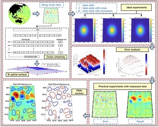
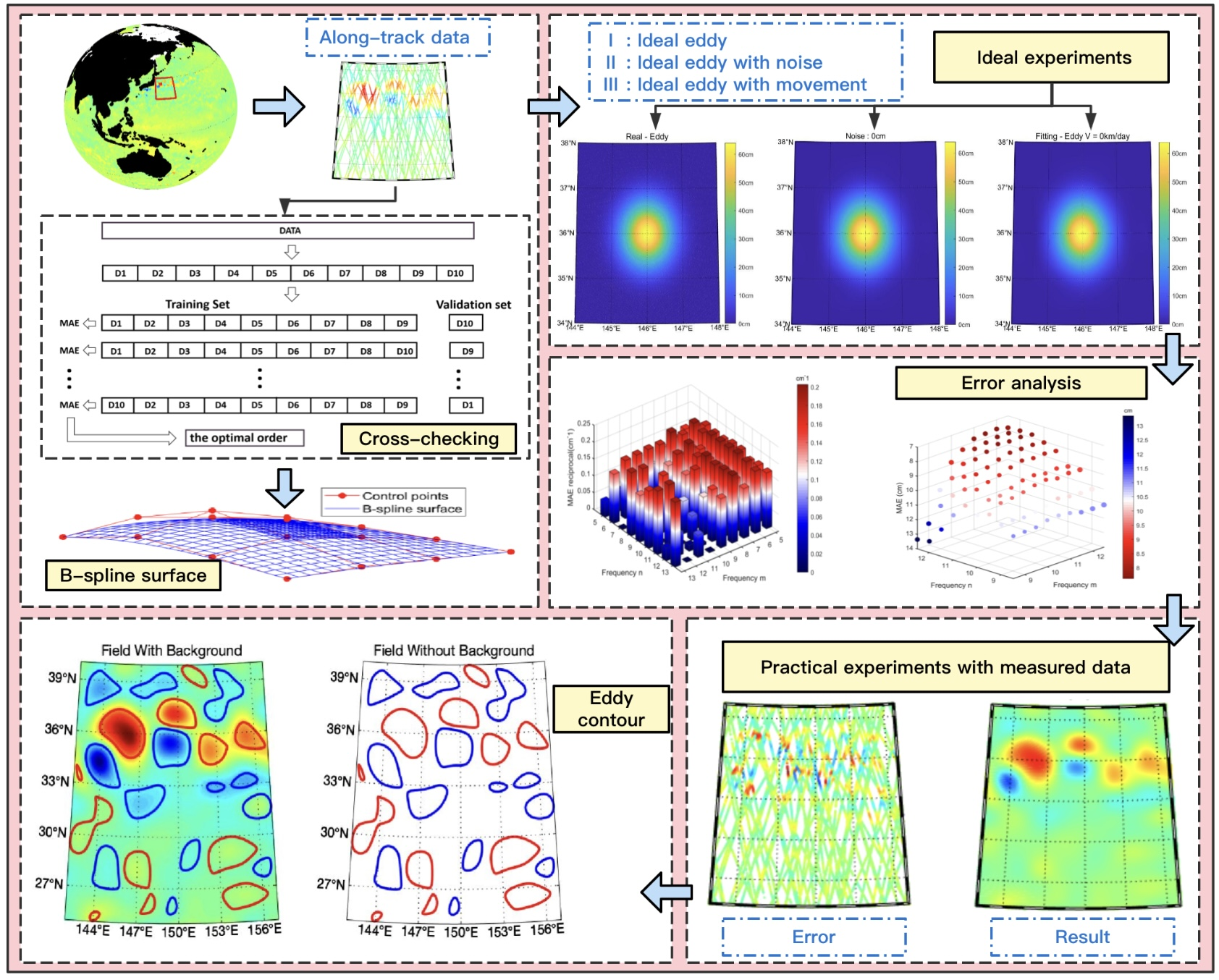
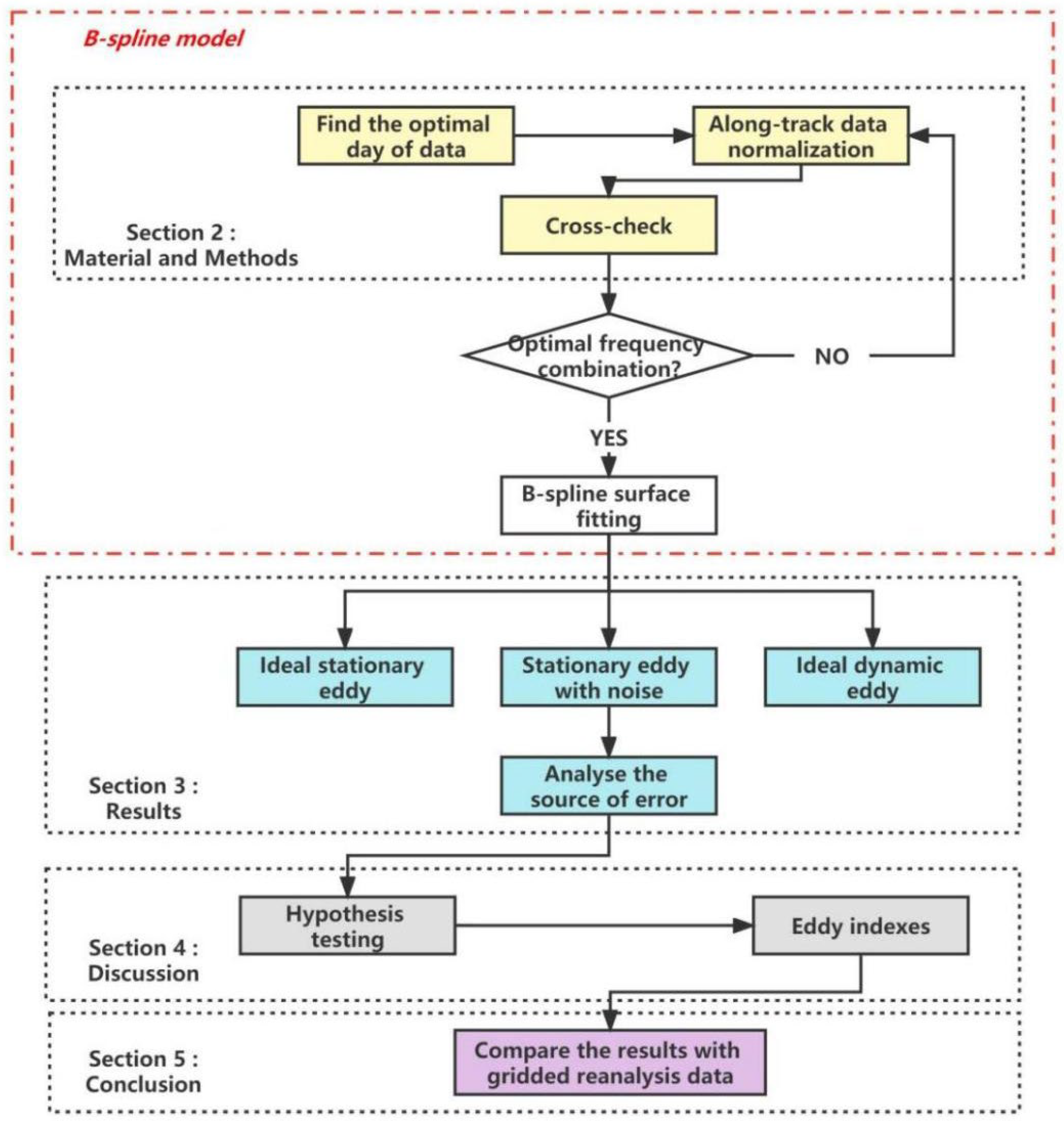
2. Materials and Methods

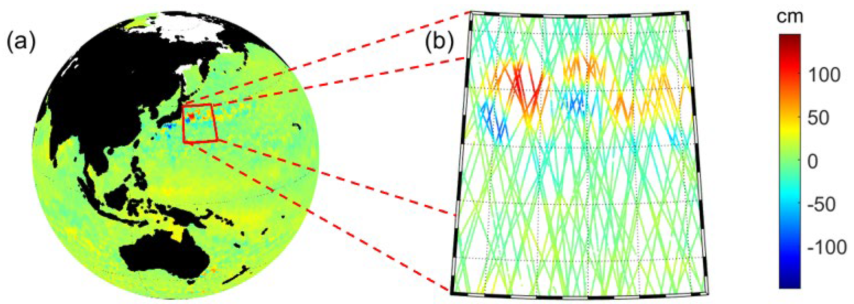
2.1. SLA Data

The along-track SLA data we used in this work is derived from the near-real-time (NRT) products distributed by CMEMS (Copernicus Marine and Environment Monitoring Service, https://marine.copernicus.eu/, accessed on 27 April 2022), which includes data (L3) from six altimeters, i.e., Saral/AltiKa, Cryosat-2, HY-2B, Jason-3, Sentinel-3A, and Sentinel-3B. These data are denoised by lowpass filtering and corrected by dynamic atmospheric correction to reflect the initial field of sea surface preferably. To reveal the superiority of the B-spline surface fitting model, we select the 9-day along-track data ranging from 1 March 2022 to 9 March 2022 and an area of 15° × 15° (25°S–40°N and 142–157°E) located in the Northwest Pacific Ocean as the study object. In this area, we conduct ideal experiments with simulated data and practical experiments with measured data, successively. The geographic location of the study area and distribution of the along-track data are shown in Figure 2, and the descriptive introduction to the SLA data in the study area is shown in

Table 1. Descriptive introduction to the SLA data.

Sample	Coverage	Range	Timer Series	Level	Type
SLA	North–West Pacific	25–40°N 142–157°E	2022,03,01–2022,03,09	3	NRT

.

2.2. Methods

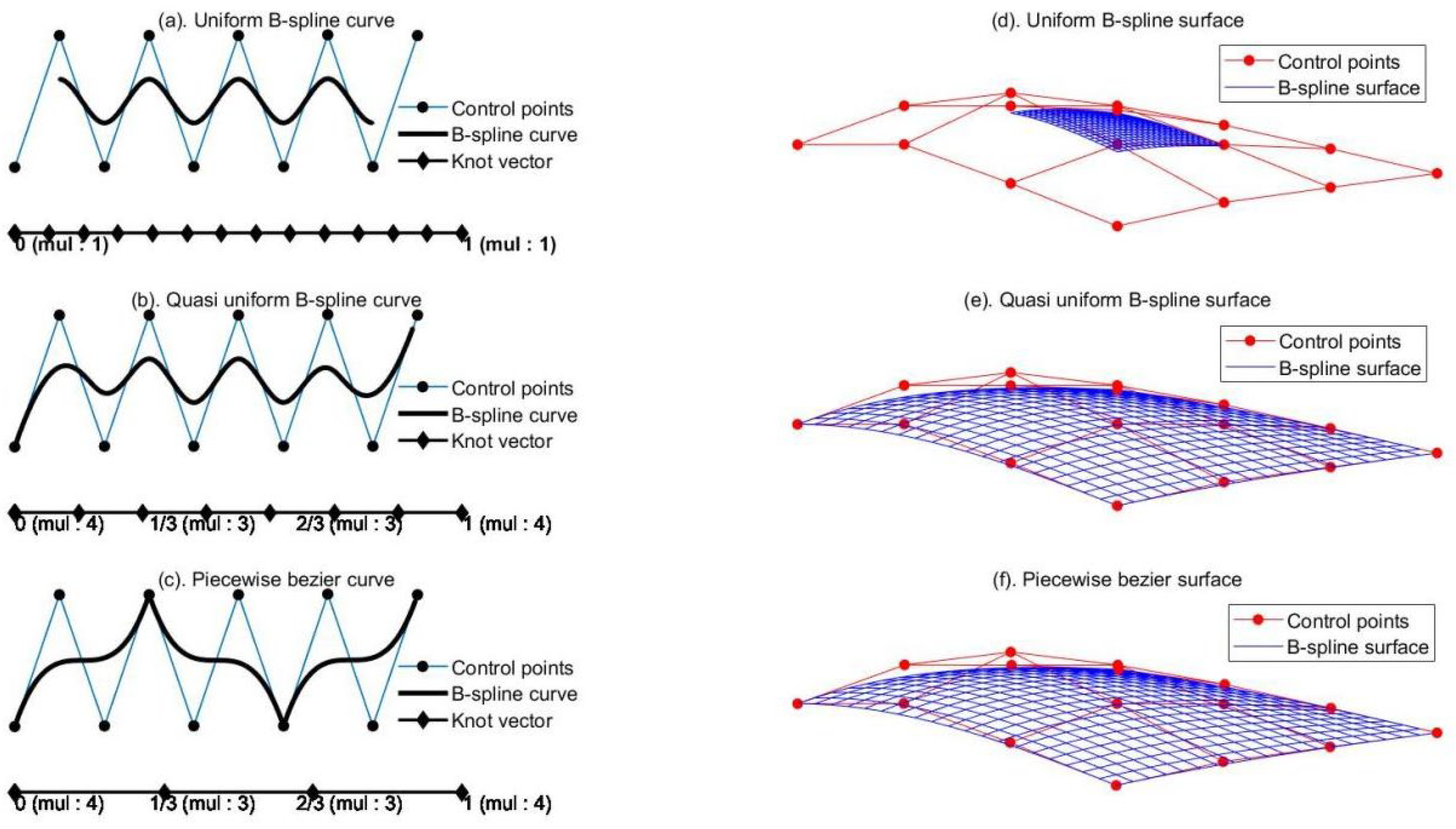
2.2.1. B-Spline Surface

Bezier proposed a method of constructing curves by control polygons in 1962, which became known as the Bezier curve. However, the curve’s local flexibility is poor, and the shape of the curve will change greatly because of the change in the position of any control point.

To solve problems with the Bezier curve, Cox [18] and De Boor [19,20] proposed replacing the Bernstein basis function with the B-spline basis function to construct a B-spline curve. Compared with the Bezier curve, the B-spline curve has more local flexibility while retaining all the advantages of the Bezier curve; it has become one of the mainstream methods for shape mathematical description [21].

Assuming that there are $n+1$ control points ${\mathrm{P}}_0,{ \mathrm{P}}_1,\dots ,{ \mathrm{P}}_{\mathrm{n}}$ and a knot vector $\mathrm{U}=\left\{{\mathrm{u}}_0,{ \mathrm{u}}_1,\dots ,{ \mathrm{u}}_{\mathrm{m}}\right\}$ with $m+1$ knots, the B-spline curves determined by these $n+1$ control points can be described by Equation (2):

$$\mathrm{C}(\mathrm{u})={\displaystyle \sum _{\mathrm{i}=0}^{\mathrm{n}}{\mathrm{N}}_{\mathrm{i},\mathrm{p}}}(\mathrm{u}){\mathrm{P}}_{\mathrm{i}},0<\mathrm{u}<1$$

(2)

where $p$ is the degree of B-spline curves, and $n, m,$ and $p$ must satisfy the constraint $m=n+p+1$. Note that we call $n$ the frequency of the B-spline curve for convenience, which means the frequency of the curve ($n)$ is conceptually equivalent to the number of control points ($n+1$). In numerical terms, frequency (n) is one less than the number of control points ($n+1$).

The knot vector $U$ is a set of non-decreasing numbers, that is, ${\mathrm{u}}_0<{\mathrm{u}}_1<\mathrm{\dots }<{\mathrm{u}}_{\mathrm{m}}$, $\left[{\mathrm{u}}_{\mathrm{i}} ,{ \mathrm{u}}_{\mathrm{i}+1}\right)$ is the ith node span. Note that the left and right endpoints of the node span may be equal, which means some node spans are zero, or rather, they do not exist. If a node repeatedly appears k times, the repeatability of this node is denoted as k [21]. In our study, it is stipulated that ${\mathrm{u}}_0$ = 0, ${\mathrm{u}}_{\mathrm{m}}$ = 1, which means the definition domain of the B-spline curve (surface) is the closed interval [0, 1].

If the knot vector is evenly distributed, as shown in Figure 3a, the B-spline curve generated by control points will not have any contact with the first and last edge of the control polygon, and this type of B-spline curve is called the open B-spline curve [21]. According to the different distribution of knots in the knot vector, B-spline curves are mainly divided into two types: one is the quasi-uniform B-spline curve, as shown in Figure 3b, whose inner knots are evenly distributed and the repeatability of knots (knots at both ends) are $p+1$, the other is the piecewise Bezier curve, as shown in Figure 3c; its inner knots’ repeatability is $p$, the repeatability of knots at both ends is $p+1$, and the positive integer multiples of degree $p$ must be equal to the number of control points ($n+1$) minus one, namely $p=n$.

In this study, the quasi-uniform B-spline curve is selected to eliminate the problem of poor fitting effect at the boundary.

${\mathrm{N}}_{\mathrm{i}, \mathrm{p}}$ is the pth-degree B-spline basis function corresponding to the ith node span, its Cox-De Boor recursion [18,19,20] is defined by Equations (3) and (4):

$${\mathrm{N}}_{\mathrm{i},0}(\mathrm{u})=\left\{\begin{array}{ll}1\hfill & {\mathrm{if} \mathrm{u}}_{\mathrm{i}}<\mathrm{u}<{\mathrm{u}}_{\mathrm{i}+1}\hfill \\ 0\hfill & \mathrm{otherwise} \hfill \end{array}\right.$$

(3)

$${\mathrm{N}}_{\mathrm{i},\mathrm{p}}(\mathrm{u})=\frac{\mathrm{u}-{\mathrm{u}}_{\mathrm{i}}}{{\mathrm{u}}_{\mathrm{i}+\mathrm{p}}-{\mathrm{u}}_{\mathrm{i}}}{\mathrm{N}}_{\mathrm{i},\mathrm{p}-1}(\mathrm{u})+\frac{{\mathrm{u}}_{\mathrm{i}+\mathrm{p}+1}-\mathrm{u}}{{\mathrm{u}}_{\mathrm{i}+\mathrm{p}+1}-{\mathrm{u}}_{\mathrm{i}+1}}{\mathrm{N}}_{\mathrm{i}+1,\mathrm{p}-1}(\mathrm{u})$$

(4)

where $\frac{0}{0}=0$. After calculating ${\mathrm{N}}_{\mathrm{i}, 0}$ and ${\mathrm{N}}_{\mathrm{i}+1 , 0}$, ${\mathrm{N}}_{\mathrm{i}, 1}$ can be obtained. All the B-spline basis functions can be calculated iteratively in this manner.

The smoothness of a B-spline curve depends on its degree $p$. In most instances, the smoothness of the curve improves with increasing degree p, but so does its computational complexity. In careful consideration of the smoothness and computational complexity of the curve, cubic B-spline curves are selected in this study, namely $p=$3.

Based on the above cubic quasi-uniform B-spline curves, the bicubic quasi-uniform B-spline surface (hereinafter, this surface is also referred to as B-spline surface for succinctness) is described as follows:

Assuming that a three-dimensional lattice $\mathrm{V}$ contains $\left(m+1\right)\times \left(n+1\right)$ control points (in other words, the frequency of one direction is $m$ and the frequency of the other direction is n in an orthogonal space), the B-spline surface $\mathrm{S}$ determined by the lattice $\mathrm{V}$ is a surface composed of $\left(m-2\right)\times \left(n-2\right)$ spatial control lattice ${\mathrm{V}}_{ \mathrm{i}, \mathrm{j}}$ which have $4\times 4$ control points spliced under the principle of ${\mathrm{C}}^2$ continuity [22]. Each surface block is represented by cubic B-spline curves in two directions which are $\mathrm{u}$ (zonal) and $\mathrm{v}$ (meridional); the surface S can be defined as Equation (5):

$$\mathrm{S}={\displaystyle \sum _{\mathrm{ii}=0}^{\mathrm{m}-2}{\displaystyle \sum _{\mathrm{jj}=0}^{\mathrm{n}-2}{\mathrm{S}}_{\mathrm{ii},\mathrm{jj}}}}(\mathrm{u},\mathrm{v})={\displaystyle \sum _{\mathrm{i}=0}^3{\displaystyle \sum _{\mathrm{j}=0}^3{\mathrm{V}}_{\mathrm{i},\mathrm{j}}}}{\mathrm{N}}_{\mathrm{i},3}(\mathrm{u}){\mathrm{N}}_{\mathrm{j},3}$$

(5)

where $\mathrm{u}$ and $\mathrm{v}$ are in the interval [0, 1], and ${\mathrm{N}}_{\mathrm{i}, 3}\left(\mathrm{u}\right)$ and ${\mathrm{N}}_{\mathrm{j}, 3}\left(\mathrm{v}\right)$ are cubic B-spline basis functions in the $\mathrm{u}$ and $\mathrm{v}$ directions as shown in Equations (3) and (4). Combining m-2 surface blocks in the u direction with n-2 surface blocks in the v direction, the bicubic B-spline surface determined by lattice V can be constructed. Similarly, depending on the different knot vectors in the direction u and v, bicubic B-spline surfaces can also be mainly divided into a uniform bicubic B-spline surface (Figure 3d), a quasi-uniform bicubic B-spline surface (Figure 3e), and a piecewise Bezier surface (Figure 3f).

In consideration of the smoothness, computational complexity, and edge-fitting effect of the surface, the quasi-uniform bicubic B-spline surface is selected in our study.

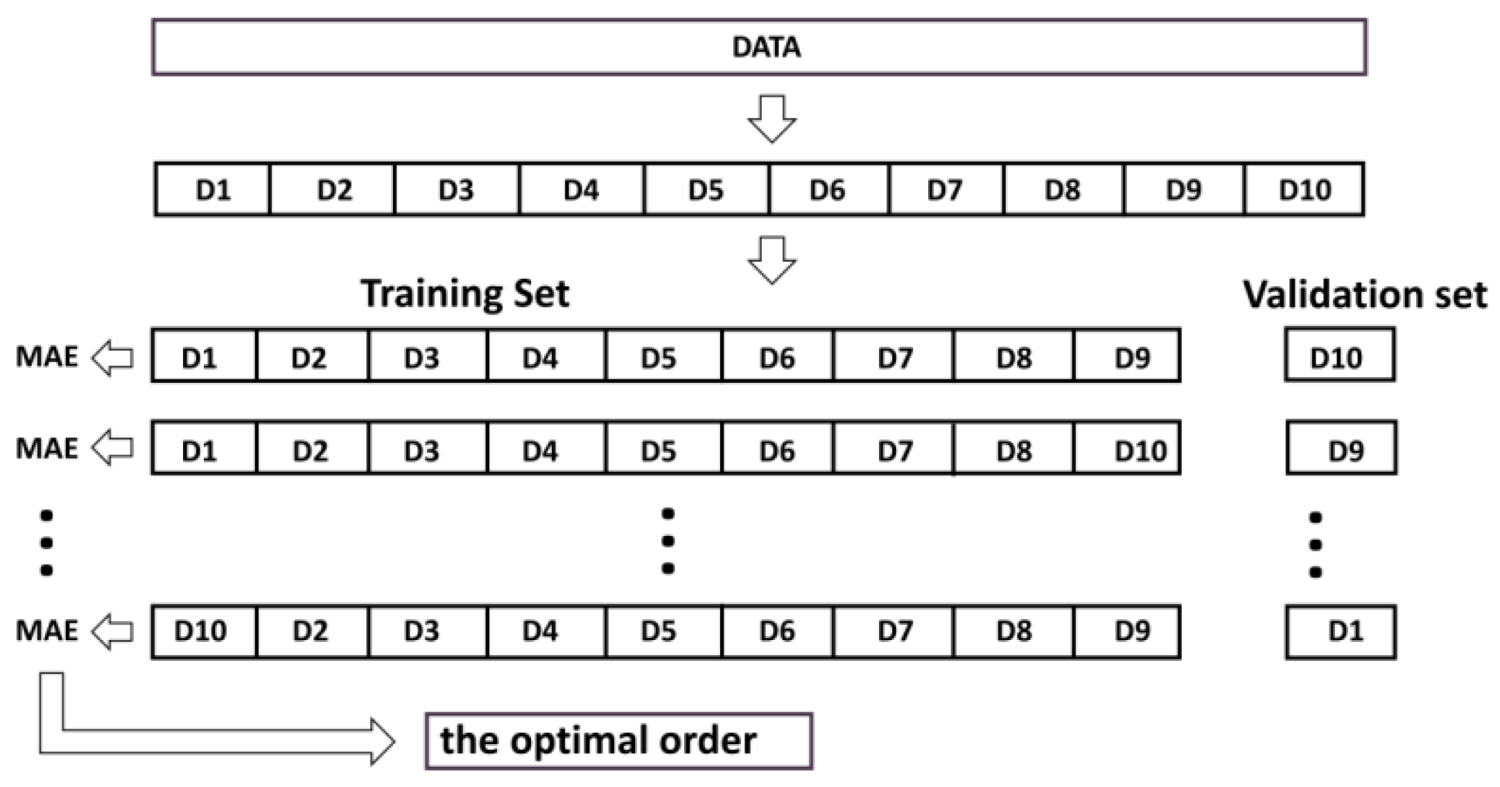
2.2.2. Cross-Checking

Before fitting the surface, we must determine the number of control points in the lattice V, or rather, determine the zonal frequency m and the radial frequency n. The frequencies m and n have an enormous influence on the fitting results, as it is easy to underfit when the frequency is too low, while over-fitting will result when the frequency is too large. To avoid these situations, the cross-check method is used to determine the number of control points in the lattice $\mathrm{V}$.

The process of cross-checking is dividing the data set into two parts: the training set and the validation set. The cross-check method can be further divided into the following four categories: Hold-hot [23], leave-one-out [24], leave-p-out [25], and K-fold [26] cross-checking; the main difference lies in the different ways of dividing data sets into training sets and validation sets.

As is shown in Figure 4, we select a 10-fold cross-check in careful consideration of computational efficiency and fitting accuracy. The along-track data set is randomly divided into ten parts (Note that there is more than one way to divide the data set, and this study adopts the way of random division), nine of them are used as training sets, and the last one is used as the validation set. Firstly, we change the number of control points in the training set (that is, changing frequency m and n). Secondly, we import the data of the validation set into the model developed by training sets corresponding to different frequency combinations; then, the model will return the mean absolute error (MAE) of the validation set. In the end, we transform a data set in the training set into a validation set, and the cross-check is repeated ten times to calculate the MAE corresponding to the same frequency combination in the cross-check. The frequency combination corresponding to the minimum MAE is the optimal frequency combination.

2.2.3. Surface Fitting

In the case that the number of control points in the lattice is determined, which means m and n are determined, fitting a quasi-uniform bicubic B-spline surface means finding a quasi-uniform bicubic B-spline surface that meets the minimum sum of error squares from all known data points $\mathrm{Q}\left(\mathrm{u},\mathrm{v}\right)$ to the B-spline surface:

$$\min {\left(\mathrm{Q}(\mathrm{u},\mathrm{v})-{\displaystyle \sum _{\mathrm{ii}=0}^{\mathrm{m}-2}{\displaystyle \sum _{\mathrm{jj}=0}^{\mathrm{n}-2}{\mathrm{S}}_{\mathrm{ii},\mathrm{jj}}}}(\mathrm{u},\mathrm{v})\right)}^2$$

(6)

In our study, the known data points $\mathrm{Q}\left(\mathrm{u},\mathrm{v}\right)$ are the SLA along-track data. The third-degree basis functions ${\mathrm{N}}_{\mathrm{i}, 3}\left(\mathrm{u}\right){ \mathrm{and} \mathrm{N}}_{\mathrm{j}, 3}\left(\mathrm{v}\right)$ in ${\mathrm{S}}_{\mathrm{ii},\mathrm{jj}}$ can be solved by Equation (4), then the problem changes into the least square problem. By solving the minimum value of Equation (6), the value of each control point in the lattice V can be solved (namely, ${\mathrm{V}}_{\mathrm{i}, \mathrm{j}}$ in Equation (5)).

When the number of control points in lattice V (namely, m and n are determined), the value of each control point (namely, ${\mathrm{V}}_{\mathrm{i}, \mathrm{j}}$) and basis functions (namely, ${\mathrm{N}}_{\mathrm{i},3}\left(\mathrm{u}\right){ \mathrm{and} \mathrm{N}}_{\mathrm{j},3}\left(\mathrm{v}\right)$) are determined, the optimal B-spline surface corresponding to this certain SLA along-track data set can be obtained according to Equation (5).

3. Results

Multiple ideal experiments with simulated data are carried out in this section to test the identification accuracy and explore the fitting error source of one mesoscale eddy fitted by a B-spline surface. A small area of 4° × 4° is selected from the study area of 25–40°N, 142–157°E, and an anticyclonic eddy is simulated in this small area. Combined with the results of a high-resolution nested simulation of the Kuroshio extension body area by using ROMS numerical model by Zhang et al. [27], the anticyclonic eddy is planned to reach a diameter of roughly 200 km and an amplitude of 65 cm. To explore the influence of noise and eddy movement on B-spline surface fitting, three groups of contrast experiments are carried out on the simulated anticyclonic eddy. Different noise levels and different westerly movement velocities are introduced to observe the change in fitting results.

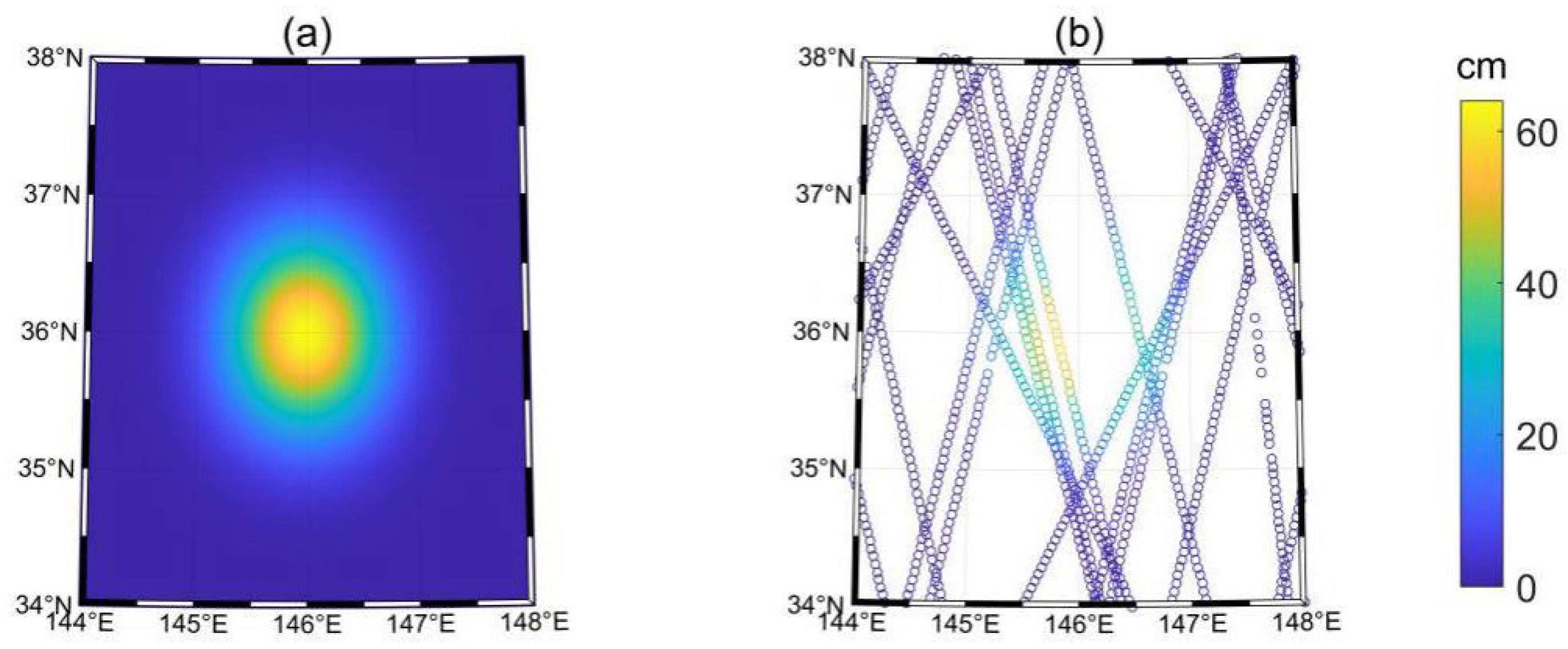
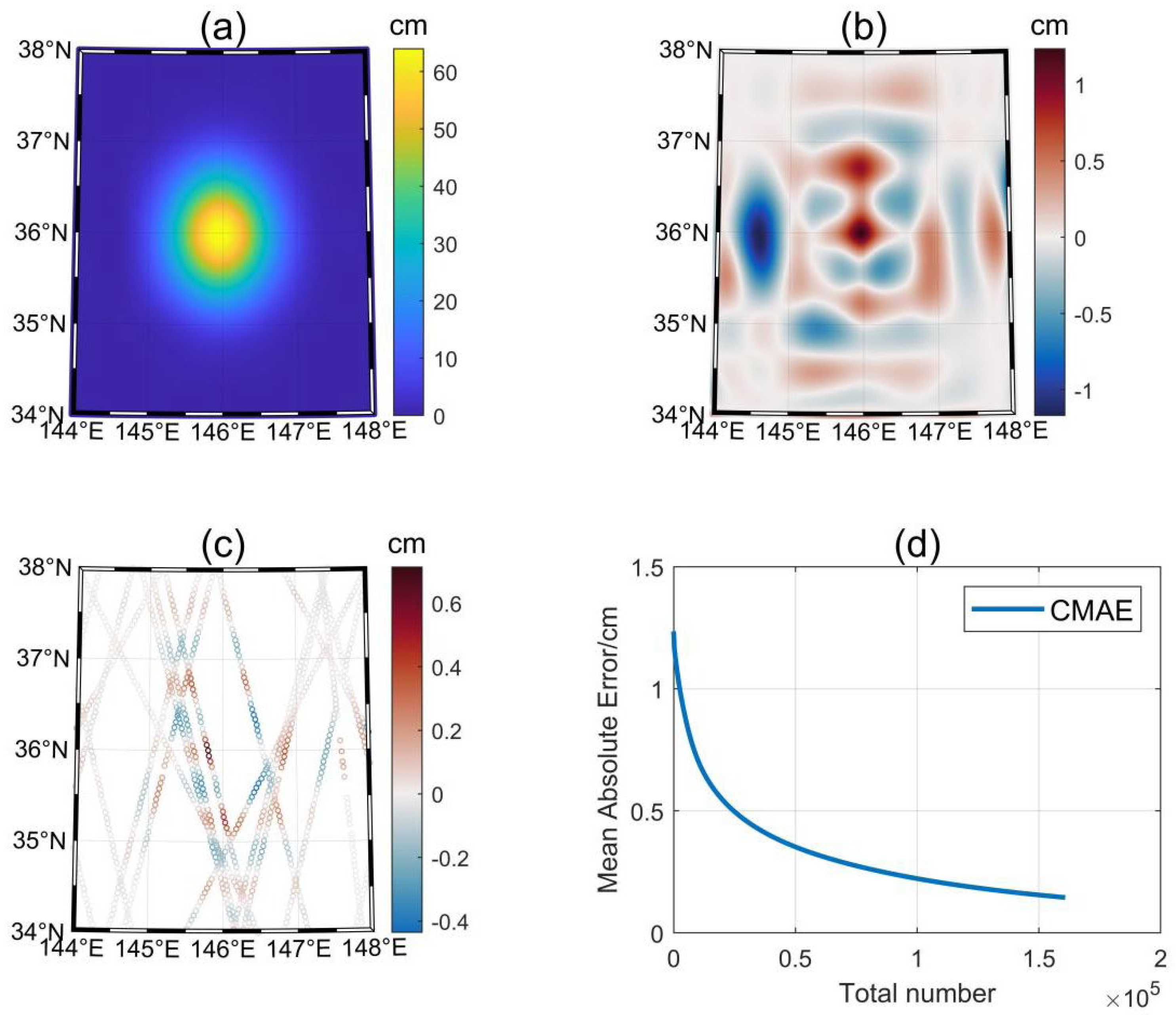
3.1. Ideal Experiment I: Ideal Stationary Eddy

The definition domain of the B-spline surface in our study is the close interval [0, 1], so data need to be normalized before starting the experiment. In our study, the min-max normalization method is selected, which is described as Equation (7):

$$\mathrm{lat} =\frac{ \mathrm{lat} -{ \mathrm{lat}}_{\min }}{{ \mathrm{lat}}_{\max }-{ \mathrm{lat}}_{\min }}, \mathrm{lon} =\frac{ \mathrm{lon} -{ \mathrm{lon}}_{\min }}{{ \mathrm{lon}}_{\max }-{\mathrm{lon}}_{\min }}$$

(7)

where ${\mathrm{lat}}_{\max },{\mathrm{lat}}_{\min }$, ${\mathrm{lon}}_{\max }$, ${\mathrm{lon}}_{\max }$ represent the maximum latitude, minimum longitude, maximum longitude, and minimum latitude, respectively.

In experiment I, the moving speed of the simulated eddy is set to zero, and no noise was introduced to explore the fitting effect of the B-spline surface on an ideal stationary anticyclonic eddy.

As shown in Figure 5a, a normally distributed eddy with a central strength of 65 cm and a diameter of nearly 200 km is generated in the area of 34–38°N, 144–148°E. The real satellite orbits in 9 days are shown in Figure 2b, which are used to generate the location of the along-track data points that are used to fit the simulated anticyclonic eddy; the along-track data are shown in Figure 5b. We change the zonal frequency m and the radial frequency n; the results of cross-checking are shown in Figure 6 and

Table 2. MAE corresponding to different frequencies (cm).

Frequency n	Frequency m
	5	6	7	8	9	10
7	5.84	5.34	6.40	6.70	7.53	28.01
8	5.86	5.03	5.86	4.95	5.41	22.79
9	5.65	5.04	6.30	5.52	7.04	14.18
10	5.63	5.02	6.30	4.93	5.69	10.32
11	6.12	5.00	6.31	5.12	8.79	13.95

.

From Figure 6 and Table 2, we can see that when the zonal frequency m is 8 and the radial frequency n is 10, the mean absolute error of the 10-fold cross-check is minimized, which is 4.93 cm.

Note that m = 8 and n = 10 are the optimal frequency combination, but the optimal frequency combination here just is the result obtained by the specific training set and verification set. A distinct set of optimal frequency combinations can be obtained if the training set and verification set are divided differently.

In the case of optimal frequency combination, the mean absolute error is 4.93 cm. However, if the frequency combination m = n = 8 is used instead of using the optimal frequency combination, the mean absolute error is 4.95 cm, whose value of the error is only 0.02 cm higher than the error corresponding to the optimal frequency combination, a change of only 0.4%. Thus, it can be considered that there is no significant difference in using the combination of frequency m = n = 8 and frequency m = 8, n = 10. The frequency combination m = n = 8 is not the optimal frequency, but it is a feasible frequency. In the following sections, to facilitate the analysis of the fitting effect, the optimal frequency combination is used to display the fitting result.

Figure 7a shows the B-spline surface fitting result of the eddy by using the along-track data, which is shown in Figure 5b. Intuitively, there is no obvious difference between the fitting eddy and the simulated eddy in Figure 7a. In this 4° × 4° area, there are 1060 along-track data points; we select absolute error as an evaluation index to analyze error because most of the data-point values are close to zero. The whole-fitting absolute error distribution is shown in Figure 7b, the absolute error distribution of the along-track data is shown in Figure 7c, and its cumulative absolute error curve (CMAE) is drawn in Figure 7d. We have conducted a qualitative analysis and quantitative analysis of error distribution, respectively.

It can be seen from the Figure 7b that, although the overall distribution of the absolute error is irregular due to the irregular spatial distribution of the data set shown in Figure 7c, the absolute error also presents a symmetric distribution of zonal and radial directions to a certain extent as a result of the existence of symmetry in the eddy itself.

As is shown in Figure 7c, the maximum absolute error of the fitting result is 0.72 cm, which appears in the central region of the eddy in Figure 7b. The average absolute error of the whole field is 0.08 cm, which is nearly three orders of magnitude lower than the central strength of the simulated eddy. Combined with the distribution in Figure 5b, it can be seen that there are no along-track data at the edge of the eddy central region, and the absolute errors in these areas are large. Therefore, from ideal experiment I, we consider that the absence of data points in some areas will lead to the occurrence of large errors in this area.

Analysis of experiment I leads to the conclusion that, for a stationary eddy, the B-spline surface fitting effect is good, and the eddy can be fitted accurately from the along-track data. The determination of the optimal frequency combination depends on the distribution of the training set and validation set in cross-checking. There is only one optimal frequency combination, although there may be more than one feasible frequency combination. The best frequency combination has an average absolute fitting error of 0.08 cm, which is within acceptable bounds.

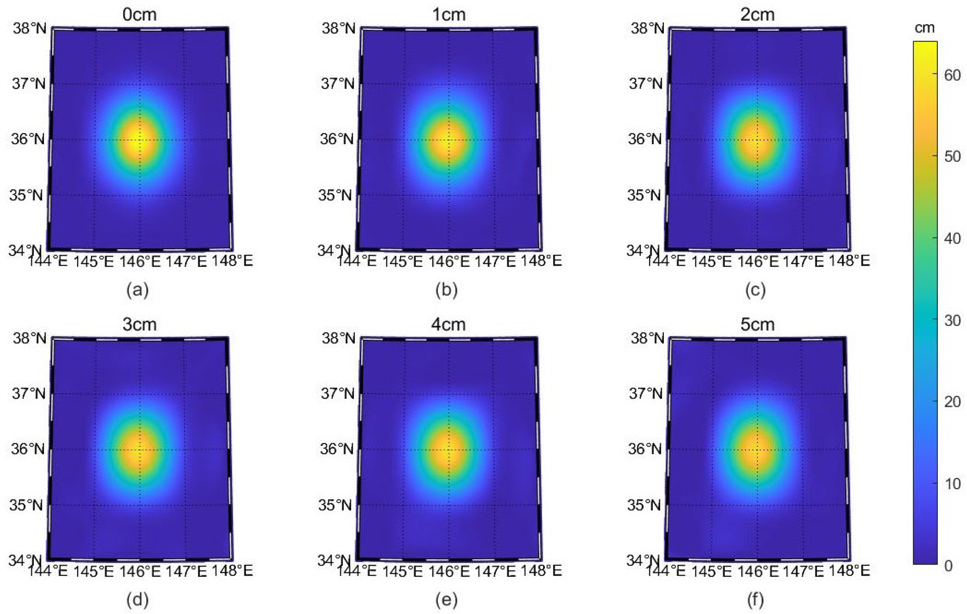
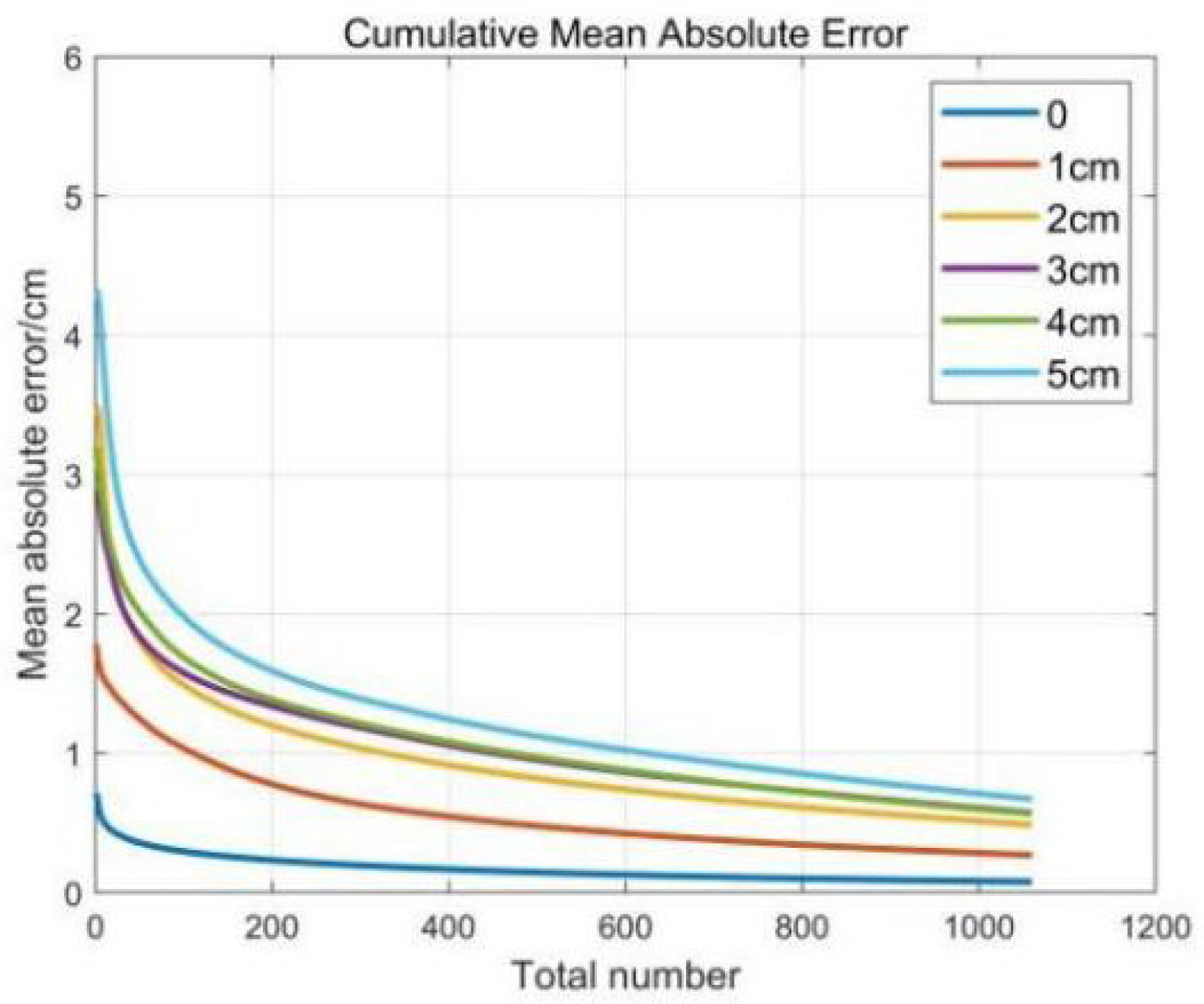
3.2. Ideal Experiment II: Stationary Eddy with Noise

To examine how noise affects the result of B-spline surface fitting, ideal experiment II was carried out, introducing different levels of noise for the simulated stationary eddy and observing the change of B-spline fitting results with the optimal frequency combination.

Figure 8a shows the state of the simulated eddy without noise; the optimal frequency combination of the B-spline surface may change with different levels of noise. Figure 8b–f shows the fitting results of the B-spline surface corresponding to the optimal frequency combination after 1–5 cm of random noise is introduced into the along-track data, respectively. Qualitatively, Figure 8 shows that the profile of the fitting eddy does not change significantly compared with the simulated stationary eddy, but its central strength tends to decrease with the increase in noise.

To quantitatively observe the changes in the fitting results, the cumulative absolute error curves of data points under different noise levels are presented in Figure 9; the corresponding cumulative absolute error change is shown in

Table 3. The value of the cumulative absolute error under differernt noise levels.

Noise (cm)	Total Number
	10%	20%	40%	60%	80%	100%
0	0.29	0.23	0.16	0.12	0.10	0.08
1	1.02	0.76	0.53	0.41	0.33	0.27
2	1.46	1.18	0.89	0.71	0.59	0.49
3	1.56	1.32	1.03	0.84	0.69	0.57
5	1.95	1.56	1.21	0.99	0.82	0.67

.

Under the same level of noise, the mean absolute error with the same percentage of total volume increases gradually. The mean absolute error increases from 0.08 cm without noise to 0.67 cm with 5 cm random noise. Although the absolute errors of certain data points are significantly enhanced when a random error of 1–5 cm is introduced, the average absolute error of the entire field increases only very little, reaching a maximum value of 0.67 cm.

We can therefore conclude that noise would have a certain impact on the result of B-spline surface fitting. Information loss relies on the quantity of noise being introduced; as noise levels rise, more actual information will be lost in the fitting eddy.

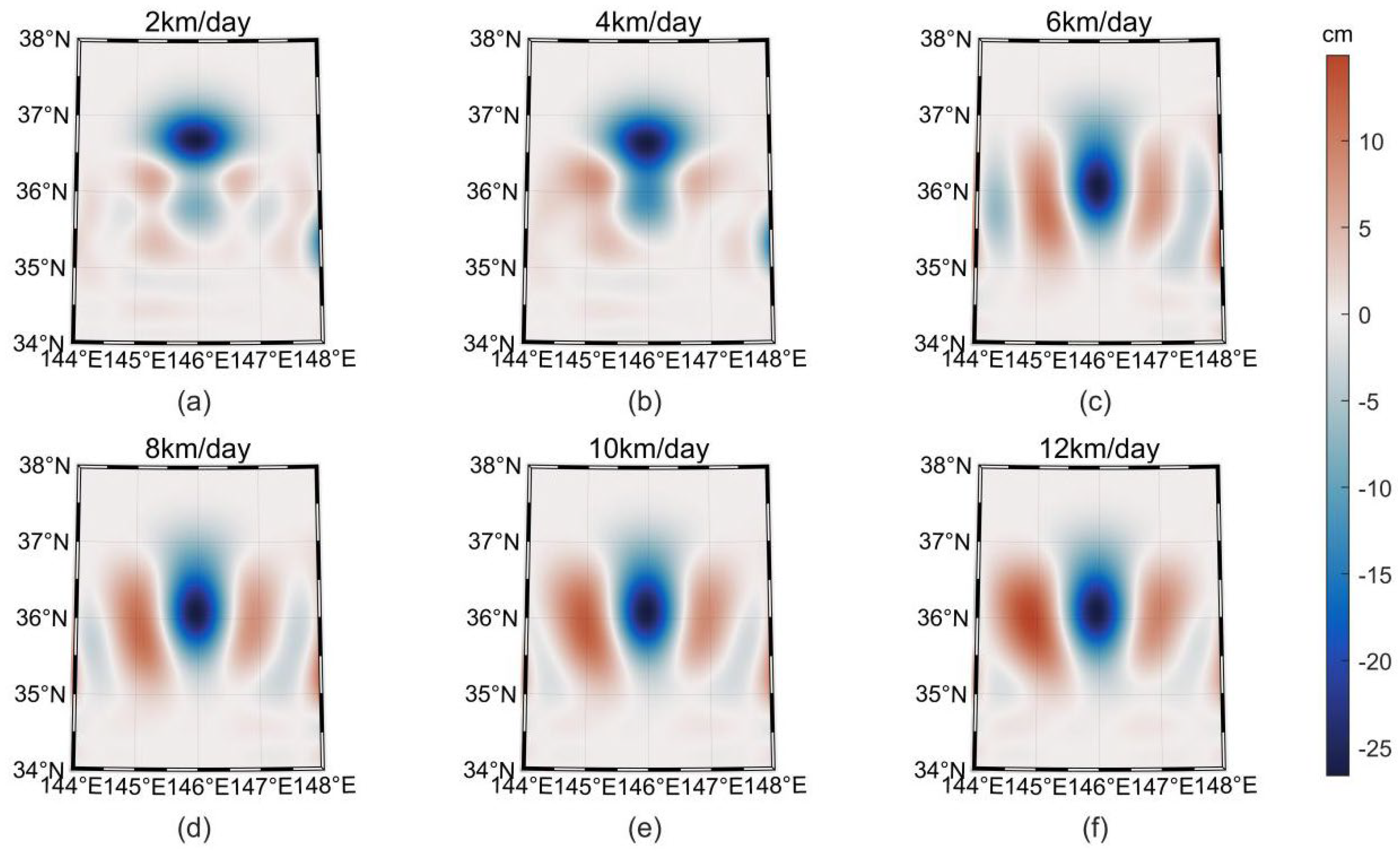
3.3. Ideal Experiment III: Ideal Dynamic Eddy

In ideal experiment III, the radial velocity of the eddy was set to 0.2 km/day. The westerly moving velocity of North Pacific mesoscale eddies ranges from 0 to 12 km/day. Therefore, the westerly moving velocity of the simulated eddy is set to range from 0 to 12 with a step size of 2 km/day, and the fitting results of the B-spline surface under the optimal frequency combination corresponding to different westerly moving velocities are present in Figure 10.

The absolute error distribution changes are shown in Figure 11. When the westerly moving speed is 2 km/day, the fitting eddy is close to the simulated eddy, and the maximum fitting error is 15 cm, which appears in the position slightly above the center of the eddy. When the westerly movement velocity gradually increases to 6 km/day, the zonal range of the fitting eddy becomes larger, the maximum value of the fitting error increases, the maximum value region moves to the center of the eddy, and the center strength of the fitting eddy decreases, the errors mainly appear in the center of the eddy and its two sides. When the westerly movement velocity is further increased to 12 km/day, it is found that the zonal range of the fitting eddy is further expanded, the error distribution becomes “low at the center and high at the two sides”, and the center’s error and zonal errors increase with the increase in the eddy’s movement velocity.

Analyzing the cause, the movement of the eddy will lead to the values of two data points with similar spatial distances greatly differing at different times. In this experiment, it is shown that, for two data points that are on different days, but have close space distance, due to the movement of the eddy, the previous day’s data point is located in the center of the eddy, while the data point from the next day is at the edge of the eddy, making the data values differ greatly in eddy strength, namely 65 cm; thus, increasing the eddy fitting error. This phenomenon occurs mostly in the edge region of the eddy.

However, in the central region of the eddy, namely the area near 36°N, 146°E, if the eddy does not move, the altimeter can only obtain the high-value point of the sea surface height caused by the convergence of seawater in this area. However, as the eddy moves to the west, the edge region of the eddy passes through the area of the central region, and the altimeter can obtain low-value points of the edge region of the eddy in the area. The influence of these low-value points on the fitting eddy reduces the intensity of its center.

The above two reasons explain why eddy movement will lead to frequent fitting errors occurring in the eddy’s central region and two sides, and the strength of the fitting eddy’s center is lower than that of the simulated eddy’s center. This error and the effect on the strength of the center will increase as the movement of the simulated eddy increases.

To quantitatively analyze the change of this error, the cumulative absolute error distribution curve at different westerly movement speeds is drawn, as shown in Figure 12, and the corresponding cumulative errors are shown in

Table 4. The value of the cumulative absolute error at different westerly movement speeds.

V	Total Number
	10%	20%	40%	60%	80%	100%
0	0.29	0.23	0.16	0.12	0.10	0.08
2	5.14	3.56	2.14	1.50	1.14	0.91
4	6.62	4.74	2.84	1.97	1.50	1.20
6	8.20	5.82	3.64	2.58	1.97	1.58
8	9.76	6.87	4.25	2.98	2.27	1.82
10	11.49	8.14	4.97	3.48	2.65	2.12
12	13.25	9.47	5.80	4.07	3.10	2.49

.

When the westerly movement velocity of the eddy increases from 0 to 12 km/day, the mean absolute error rises from 0.08 to 2.49 cm. It can be seen that, when the westerly movement velocity of the eddy is too high, the B-spline surface fitting will lose a lot of real information about the eddy, making it impossible to fit the real shape of the eddy.

4. Discussion

4.1. Practical Experiments with Measured Data

From ideal experiments in Section 3, we can conclude that noise and westerly movement velocity have a great influence on the B-spline surface fitting. To explore the effect of B-spline surface fitting on real eddies, we selected an area (15° × 15°) near the Kuroshio extension body to conduct experiments based on the real along-track altimeter data.

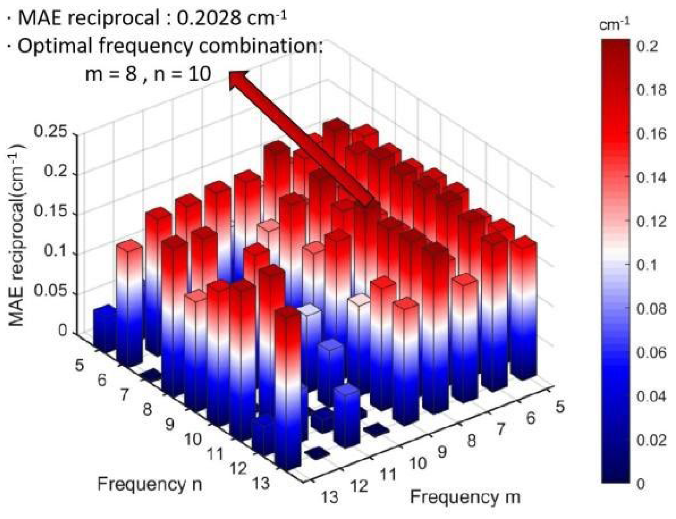
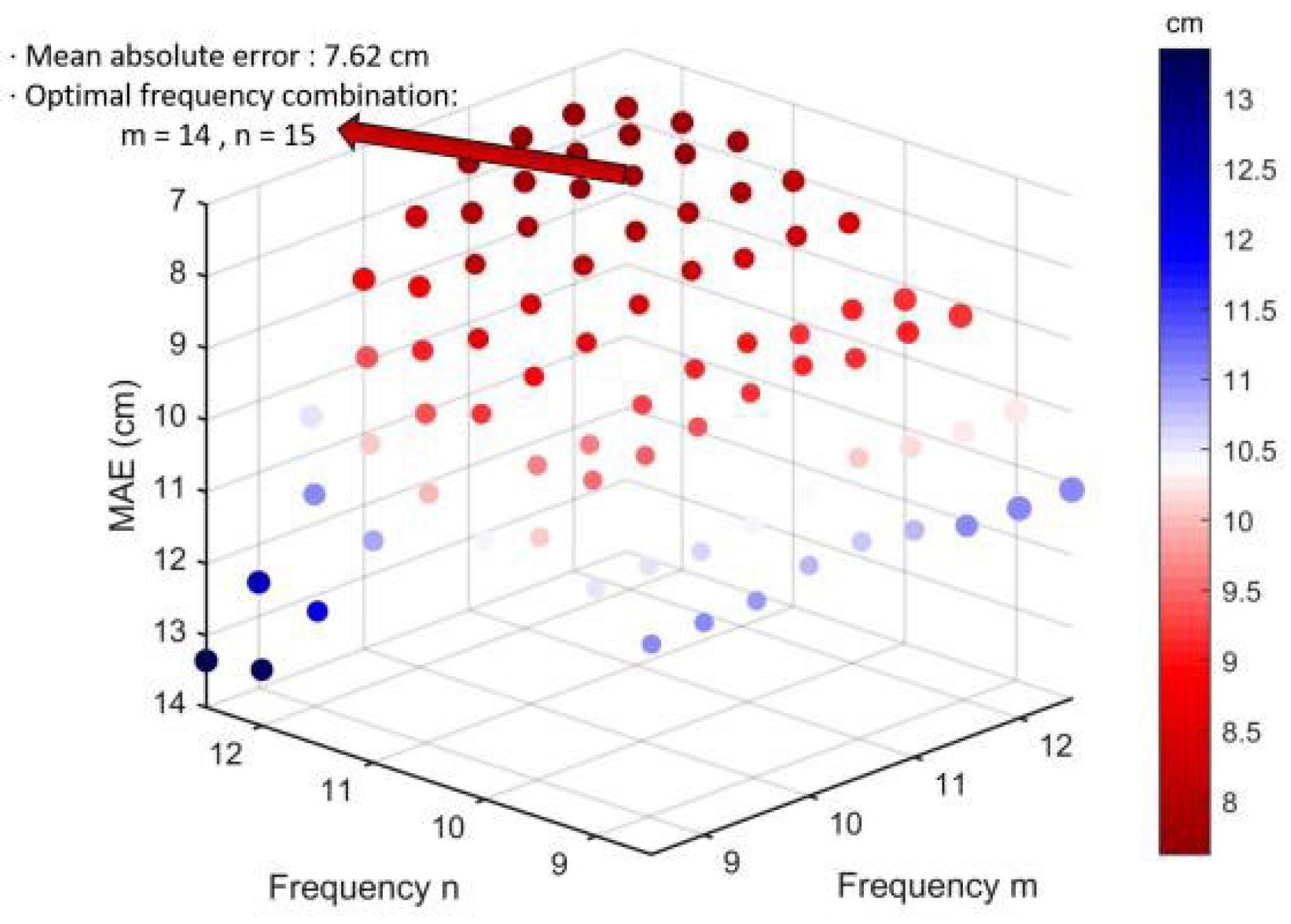
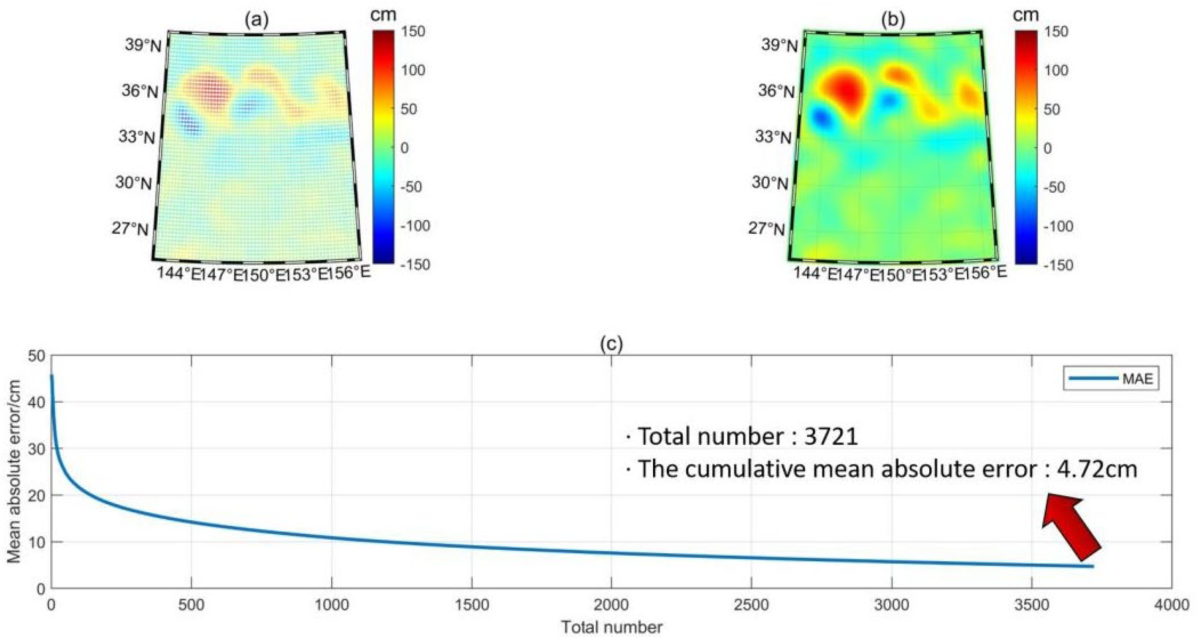
4.1.1. Determining the Optional Frequency Combination

Firstly, we need to determine the range of days of the data set for B-spline surface fitting. The fitting error increases with the number of days of data selected and the speed of the eddy’s westerly movement. If the number of days selected is too small, the B-spline surface can’t fit the eddy due to the number of given data points being too low to reflect the state of the eddy; conversely, if the number of days selected is too large, noise and the eddy’s westerly movement will further cause an increase in the fitting error.

It should be noted that different ranges of days of the dataset correspond to different optimal frequency combinations. The control variables method and cross-check mentioned in Section 2.2.2 are used in this experiment to determine the optional frequency combination. First, we made the days of the data set range from 1 to 20, then changed the zonal frequency m and radial frequency n to obtain the optimal frequency combination corresponding to different days of the dataset.

It can be seen from

Table 5. Minimum MAE corresponding to different days of data set (cm).

	Days
	5	6	7	8	9	10	11	12	13
Data Points	8781	10,042	12,797	14,763	16,108	17,746	19,942	21,413	23,119
MAE	13.24	8.77	8.11	8.04	7.62	7.67	7.74	8.05	8.19

that the B-spline surface shows the best fitting effect when the data from nine consecutive days are used, namely, when 16,108 along-track data points are selected. However, the MAE corresponding to the data from 7–11 consecutive days is very close, and the maximum MAE difference is only 0.49 cm, which only changes 6.4% relative to the MAE from 9 consecutive days. Therefore, all 7–11 days are feasible days for the dataset, and all the corresponding fitting results are acceptable. For the convenience of analysis, we select the data from nine consecutive days for further study.

Figure 13 and

Table 6. The value of the cumulative absolute error under different frequency combinations.

Frequency n	Frequency m
	11	12	13	14	15	16
12	9.60	9.32	9.09	9.00	9.15	9.08
13	8.91	8.71	8.45	8.25	8.35	8.31
14	8.64	8.43	8.16	7.96	7.97	7.96
15	9.06	8.13	7.88	7.62	7.71	7.68
16	9.41	8.70	7.94	7.78	7.66	7.67
17	10.49	8.85	8.25	7.77	7.69	7.64

correspond to each other; it can be seen that MAE reaches a minimum when m = 14 and n = 15; in this case, the lattice V contains 240 control points. However, it is similar to the case of determining the day of the dataset when m ranges from 13 to 15 and n ranges from 14 to 16; the MAE corresponding to every frequency combination does not differ greatly, with the maximum difference being only 0.5 cm, which is very small compared with real SLA along-track data. So even when ranging m from 13 to 15, n from 14 to 16, or when making the range even larger, all the corresponding frequency combinations are feasible.

In order to facilitate the subsequent analysis, we select the optional frequency combination m = 14, n = 15; the B-spline surface fitting result and the absolute fitting error are present in Figure 14a,b, respectively.

It can be seen from Figure 14b that the vast majority of the data points where the fitting error is large appear at the edge of the eddy. Combined with the conclusion of ideal experiment III, the movement of the eddy may be the cause of this phenomenon. In order to further determine whether the fitting error is within the acceptable range, we conducted hypothesis testing on the fitting error.

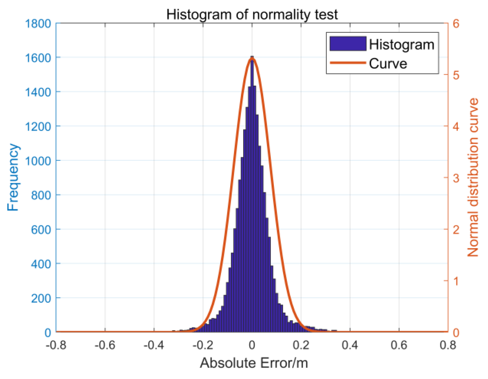
4.1.2. Hypothesis Testing

Firstly, a normality test is necessary for the fitting errors. The null hypothesis is that the fitting error conforms to the normal distribution, and the alternative hypothesis is that the fitting error doesn’t conform to the normal distribution. The result of the normality test is presented in

Table 7. Normality test (cm).

Sample	Total	Average	Skewness	Kurtosis	S–W Inspection	K–S Inspection
ERROR	16,108	−0.075	0.427	4.453	0.942 (0.000 ***)	0.067 (0.000 ***)

Note: *** represents the significance level of 1%.

.

Because the data from nine consecutive days is a large sample with far more than 5000 data points, K–S inspection has higher reliability. The result of the K–S inspection shows that p is less than 0.01, meaning the result is significant, and the null hypothesis is rejected at a 99% confidence level. So the data does not conform to a normal distribution. However, in practice, the uncertainty of the data is great, and the dataset cannot easily fit a strict normal distribution; other methods should be adopted to test the normality of the data.

As shown in Table 7, the absolute value of kurtosis of the sample data in this experiment is less than 10, and the absolute value of skewness is less than 3, which can be combined with the histogram of normal distribution and P-P diagram for further analysis. In the normal distribution histogram, if the data distribution is high in the middle and low on both sides, the more bell-shaped the data is, the stronger the normality of the data will be. In the P-P diagram, we can observe whether the points on the graph are distributed on the straight line of the theoretical distribution; if the points are distributed on the straight line, it indicates that the data approximately follows the normal distribution.

The kurtosis and skewness of the data error are 4.453 and 0.427; and, the normal distribution and P-P diagram are present in Figure 15 and Figure 16:

The normal distribution histogram shows a largely bell-shaped trend where the middle is high, and the two sides are low, and the P-P diagram shows a good fit between the accumulated probability (P) and the normal accumulated probability (P), approximately forming a straight line. Therefore, we can conclude that, although the error data is not absolutely normal, it can be accepted as a normal distribution.

On the premise of accepting the error data as a normal distribution, the single-sample t-test is performed on the data, and the test value is set to 0. The null hypothesis is that there is no difference between the fitting error and the test value. The result is shown in

Table 8. The single-sample t-test.

Test Value	Total	Standard Deviation	T	P
0	16,108	0.427	−1.398	0.162

:

It can be seen from the result of the single-sample t-test that the P is 0.162, so the null hypothesis can’t be rejected, meaning there is no significant difference between the fitting error and test value 0. Therefore, the fitting error of B-spline surface fitting can be regarded as 0, and there is no significant difference between the fitting result and the given along-track data.

4.1.3. Mesoscale Eddy Indexes

After obtaining the sea surface height anomaly fitting pattern, as shown in Figure 14a, we set a series of indexes to identify the contour of the eddy and make the display of the eddy more intuitive. We refer to Chelton’s method [2] of using pixel sets to identify the mesoscale eddy proposed in 2011, which can identify the contour of the mesoscale eddy, but not the location of the eddy core.

Combined with the method proposed by Chelton and the statistical characteristics of the global nonlinear mesoscale eddy [4], we defined the mesoscale eddy in the study area as follows:

• For an (anticyclone) cyclone eddy, the SLA data points inside the eddy are all (high) below a certain value.
• For an (anticyclone) cyclone eddy, there is at least one minimum (maximum) SLA value.
• The amplitude of the eddy is not less than 7.5 cm.
• The eddy boundary is a closed contour.
• The diameter of the eddy ranges from 50 to 400 km.

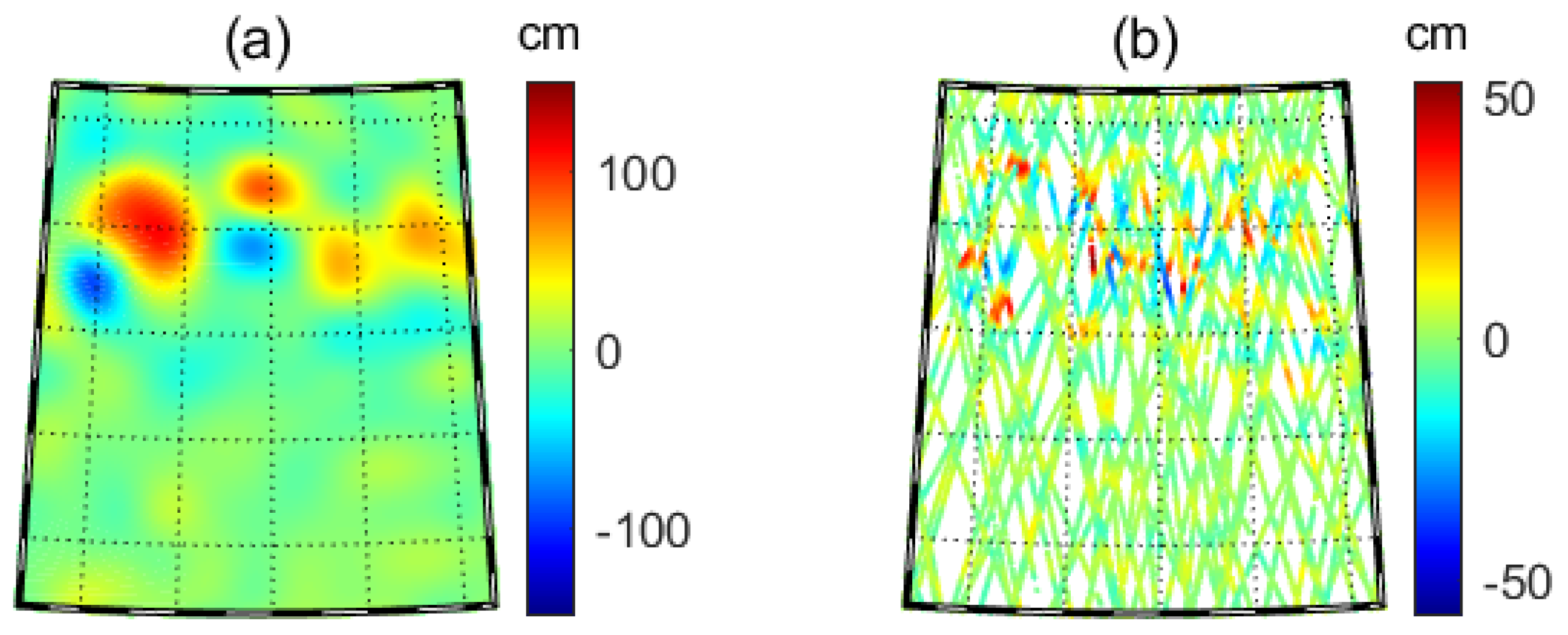
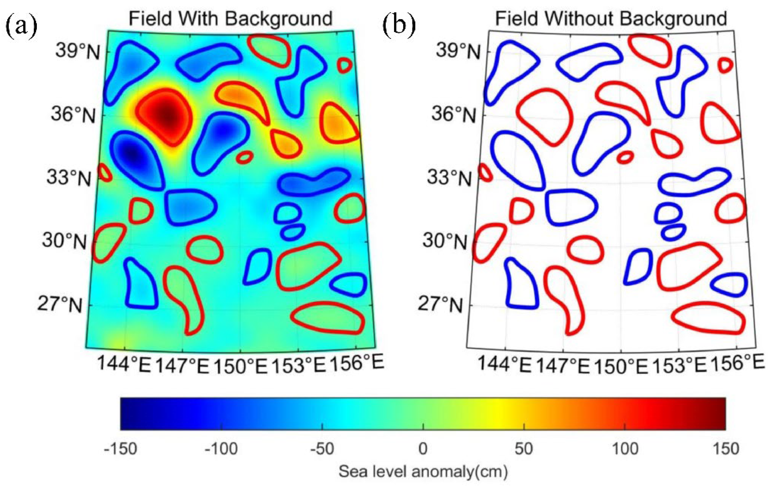
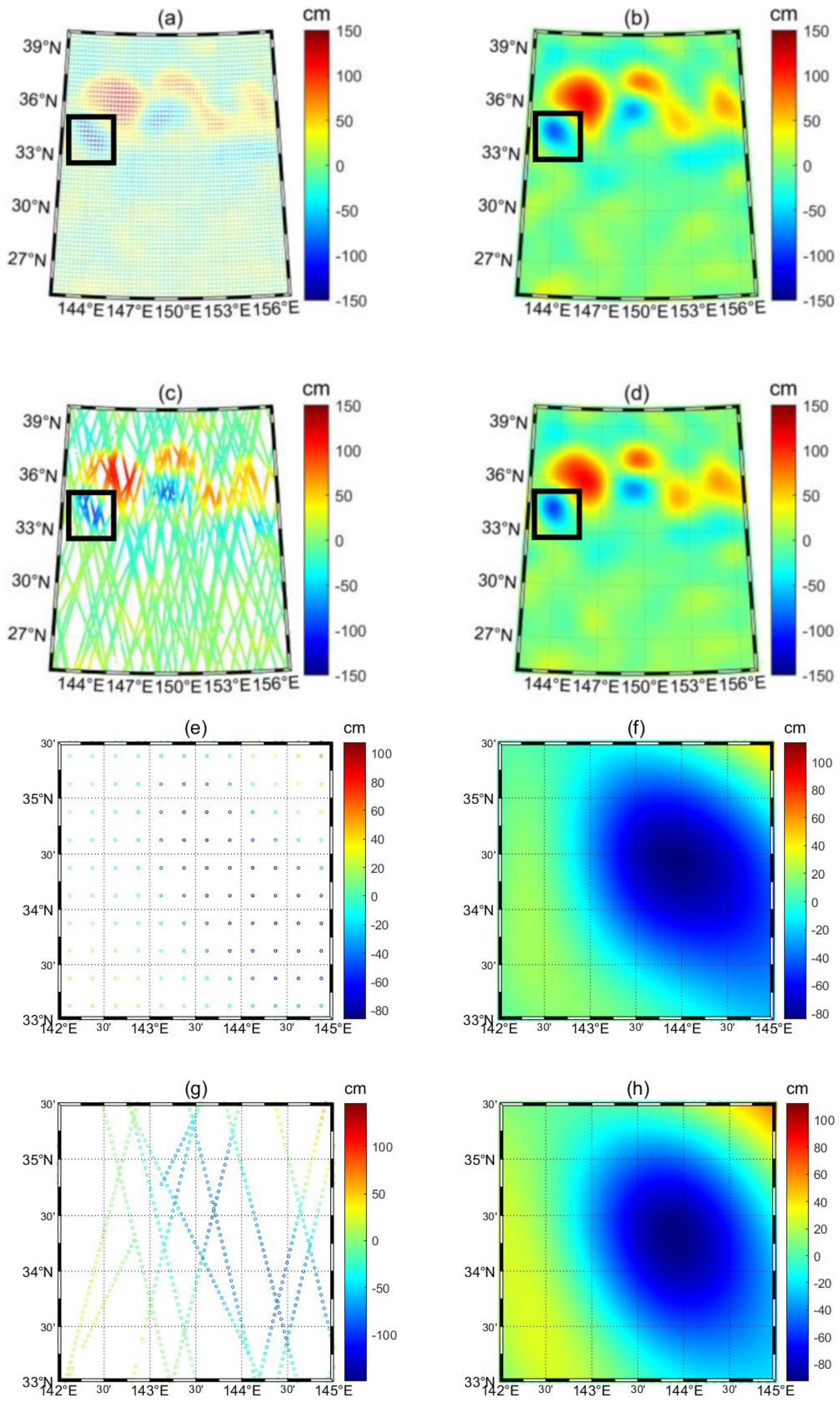
As can be seen from the above definition, the key to identifying mesoscale eddies lies in the setting of the first index: specific SLA value. We limit the range of SLA within −200 to 200 cm, and the closed SLA contour lines of cyclone eddies and anticyclone eddies are respectively searched with steps of 1 cm until the eddy formed by the contour satisfies the above five indexes.

4.2. Eddy Contours

The method and eddy indexes defined above are adopted to obtain the identification results, which are shown in Figure 17. Figure 17a contains eddy contours and the background field, while Figure 17b only contains the eddy contours. Comparing the two figures, it can be seen that the bicubic quasi-uniform B-spline fitting method can well reflect the initial field information of the sea surface. Using the data from nine consecutive days for this experiment, the identification effect is good in that it identifies 15 anticyclone eddies and 12 cyclone eddies successfully, corresponding to frequency 14 (m = 14) in the zonal direction and frequency 15 (n = 15) in the meridional direction, respectively.

However, there are still some aspects that need to be improved. For example, the mesoscale eddy contour depends on the indexes we choose, and the effect of contour recognition varies with different indexes. In our study, the mesoscale eddy indexes we set cannot distinguish between multi-core eddy structures; if two eddies’ spatial positions are too close and they share comparable characteristics, the B-spline model will identify them into the same eddy, causing a “gourd shape” structure.

4.3. Compare and Analyze the Results of Gridded Data and Along-Track Data

For the above experiments, we also briefly analyzed the fitting effect of the B-spline surface on gridded reanalysis data. SLA gridded reanalysis data with a resolution of 0.25° × 0.25° in the area of 25°S–40°N and 142–157°E from 9 March 2022, is presented in Figure 18a. The B-spline surface fitting result is shown in Figure 18b, and the corresponding cumulative absolute error curve is shown in Figure 18c.

Combining Figure 18a–c, it can be seen that the mean absolute error of all data points in the area is 4.72 cm. The resolution of the fitting result in Figure 18b is 0.01° × 0.01°; compared with the resolution of data in Figure 18a, which is 0.25° × 0.25°, its degree of visualization is better, the spatial distribution of data is denser, and there is no significant difference between the result of B-spline fitting and initial gridded data. So, we conclude that the B-spline surface can densify the spatial distribution of gridded reanalysis data and still show a good fitting effect.

The advantages and shortcomings of the data source itself must be considered. As we mentioned in the introduction, we can discuss this problem in the following aspects:

The result of B-spline surface fitting based on the gridded reanalysis data and along-track data are shown in Figure 19, where Figure 19a,c are initial gridded reanalysis data and initial along-track data of the same days in the same area, respectively, Figure 19b,d are the fitting results of corresponding B-spline surface. It can be seen from Figure 19 that there are significant differences between the spatial distribution of gridded data and that of along-track data, while the corresponding B-spline fitting results show little difference. At the same spatial position in Figure 19b,d, one data point is taken every 0.01°, and the average fitting error of all data points is 4.41 cm. That is, the fitting results of the B-spline surface based on gridded reanalysis data and along-track data showed only a 4.41 cm difference in the whole field.

A single cyclone eddy is extracted separately to conduct a more detailed comparative analysis. The position of this eddy is shown in the black box in Figure 19a–d, and the spatial distribution and fitting result corresponding to the black box are present in Figure 19e–g.

Figure 19e–h are reflecting the same cyclone eddy from the same day, but Figure 19e is the gridded reanalysis data source, Figure 19f is the corresponding fitting result; Figure 19g is the along-track data source, Figure 19h is the corresponding fitting result. Comparing the four Figures, it can be seen that the value range of the gridded reanalysis data is smaller than the along-track data. This is due to the gridded reanalysis data having been smoothed, and some extreme points have been weakened. So, the strength of the data source and corresponding fitting result from the gridded reanalysis data are weaker than those from the along-track data. In this aspect, along-track data is a more accurate data source and can reflect the actual state of the eddy better.

From the point of view of the spatial distribution of data, along-track data can be seen as a representation of a series of irregular distribution data, such as ship scatter data. Gridded reanalysis data also can be regarded as a special case of irregular distribution data, so a data processing method appropriate for handling along-track data also can be applied to gridded reanalysis data. In this aspect, the universality of the along-track data is better than that of gridded reanalysis data.

In actual ocean observations, most of the data available initially to us show an irregular spatial distribution rather than a regular gridded distribution. Time and more procedures are needed to turn the irregular spatial distribution data into gridded reanalysis data; this may lead to data hysteresis and introduce re-sampling error into results, as we discussed above. In this aspect, the along-track data has a better ability of instantaneity.

On the one hand, in terms of fitting results, for gridded reanalysis data, B-spline surface fitting can densify the spatial distribution of the data under the premise that data is not distorted; while, for along-track data, which can be seen as a representation of the irregular distribution of scatter data, B-spline surface fitting provides a new technological means in data analysis and mesoscale eddy detection.

On the other hand, in terms of the accuracy, universality, and instantaneity of the data source, the along-track data itself is a better data source than the gridded reanalysis data; results obtained from the along-track data are more representative of the practical state of the sea surface.

Therefore, it can be concluded that B-spline surface fitting has a good fitting effect on both gridded reanalysis data and along-track data.

5. Conclusions

Gridded reanalysis data, which has been widely used in ocean science for a long time, is a processed product of along-track data. However, there are few references relating to the direct use of along-track data. It is unavoidable that much initial information is lost during data reprocessing, and in actual ocean observations, the majority of the data initially accessible to us reveal an irregular spatial distribution rather than a normal gridded distribution. Thus along-track data is the better data source in terms of accuracy, universality, and instantaneity.

Aiming to exploit the advantages of along-track data sources, we encourage audiences to examine along-track data instead of gridded reanalysis data. Taking mesoscale eddy identification as an example, the B-spline surface fitting model is proposed. This innovative model can identify eddies solely based on along-track data and provides a new technical means in data analysis, ocean science, and climate change science.

To explore the influence of noise and an eddy’s westerly movement on the fitting effect, three different types of oceanic mesoscale eddies, static, static with noise, and moving without noise, are simulated; and the corresponding three ideal experiments are carried out. It is discovered that when noise and movement increase, more genuine information is lost in the process of fitting the eddy, and there is only one optimal frequency combination, although there may be more than one group of feasible frequency combinations that exist.

To examine the effect of B-spline surface fitting based on along-track data, an area of 15° × 15° near the Kuroshio extension body is selected to conduct practical experiments with measured data and analyze fitting error further. Hypothesis testing is adopted to analyze the error, and the result shows that there are no significant differences between the fitting data and initial along-track data. In order to present the contour of mesoscale eddies more intuitively, five mesoscale eddy indexes are set according to Chelton’s method and the statistical characteristics of global oceanic nonlinear mesoscale eddies. Fifteen anticyclone eddies and twelve cyclone eddies are detected successfully using this approach.

Finally, we analyze the advantages of along-track data compared to gridded reanalysis data, discuss briefly the fitting effect of B-spline surface on gridded reanalysis data, and compare it with along-track data. The result shows that B-spline surface fitting has a good fitting effect on both gridded reanalysis data and along-track data.

Mesoscale eddies are identified successfully in this paper using only SLA along-track data to identify eddies using the B-spline surface fitting model. Considering that there is more than one identification index of oceanic mesoscale eddies, such as temperature, nutrients, and other marine elements, which can reflect eddy characteristics, it is necessary to carry out more B-spline fitting experiments on other marine elements. Additionally, ship scatter data can also be integrated into the B-spline surface fitting model, which is anticipated to significantly increase the model’s recognition accuracy and efficiency.

References

1. Chen, G.; Yang, J.; Tian, F.; Chen, S.; Zhao, C.; Tang, J.; Liu, Y.; Wang, Y.; Yuan, Z.; He, Q.; et al. Remote sensing of oceanic eddies: Progresses and challenges. Natl. Remote Sens. Bull. 2021, 25, 302–322. [Google Scholar] [CrossRef]
2. Gordon, A.L.; Giulivi, C.F. Ocean eddy freshwater flux convergence into the North Atlantic subtropics. J. Geophys. Res. Ocean. 2014, 119, 3327–3335. [Google Scholar] [CrossRef]
3. Hausmann, U.; Czaja, A. The observed signature of mesoscale eddies in sea surface temperature and the associated heat transport. Deep Sea Res. Part I Oceanogr. Res. Pap. 2012, 70, 60–72. [Google Scholar] [CrossRef]
4. Chelton, D.B.; Schlax, M.G.; Samelson, R.M.; De Szoeke, R.A. Global observations of large oceanic eddies. Geophys. Res. Lett. 2007, 34, 87–101. [Google Scholar] [CrossRef]
5. Adams, D.K.; Mcgillicuddy, D.J.; Zamudio, L.; Thurnherr, A.M.; Liang, X.; Rouxel, O.; German, C.R.; Mullineaux, L.S. Surface-Generated Mesoscale Eddies Transport Deep-Sea Products from Hydrothermal Vents. Science 2011, 332, 580–583. [Google Scholar] [CrossRef] [Green Version]
6. Siegel, D.A.; Granata, T.C.; Michaels, A.F.; Dickey, T.D. Mesoscale eddy diffusion, particle sinking, and the interpretation of sediment trap data. J. Geophys. Res. Ocean. 1990, 95, 5305–5311. [Google Scholar] [CrossRef] [Green Version]
7. Wyrtki, K.; Magaard, L.; Hager, J. Eddy energy in the oceans. J. Geophys. Res. Atmos. 1976, 81, 2641–2646. [Google Scholar] [CrossRef]
8. Dong, C.; McWilliams, J.C.; Liu, Y.; Chen, D. Global heat and salt transports by eddy movement. Nat. Commun. 2014, 5, 3294. [Google Scholar] [CrossRef] [Green Version]
9. Duo, Z.; Wang, W.; Wang, H. Oceanic Mesoscale Eddy Detection Method Based on Deep Learning. Remote Sens. 2019, 11, 1921. [Google Scholar] [CrossRef] [Green Version]
10. Nencioli, F.; Dong, C.; Dickey, T.; Washburn, L.; Mcwilliams, J.C. A Vector Geometry-Based Eddy Detection Algorithm and Its Application to a High-Resolution Numerical Model Product and High-Frequency Radar Surface Velocities in the Southern California Bight. J. Atmos. Ocean. Technol. 2010, 27, 564. [Google Scholar] [CrossRef]
11. Okubo, A. Horizontal dispersion of floatable particles in vicinity of velocity singularities such as convergences. Deep Sea Res. Oceanogr. Abstr. 1970, 17, 445–454. [Google Scholar] [CrossRef]
12. Weiss, J. The dynamics of enstrophy transfer in 2-dimensional hydrodynamics. Phys. D Nonlinear Phenom. 1991, 48, 273–294. [Google Scholar] [CrossRef]
13. Isern-Fontanet, J.; Font, J.; Garcia-Ladona, E.; Emelianov, M.; Millot, C.; Taupier-Letage, I. Spatial structure of anticyclonic eddies in the Algerian basin (Mediterranean Sea) analyzed using the Okubo-Weiss parameter. Deep Sea Res. Part II 2004, 51, 3009–3028. [Google Scholar] [CrossRef]
14. Mcwilliams, J.C. The emergence of isolated coherent vortices in turbulent flow. J. Fluid Mech. 1984, 146, 21–43. [Google Scholar] [CrossRef] [Green Version]
15. Sadarjoen, I.A.; Post, F.H. Detection, quantification, and tracking of vortices using streamline geometry. Comput. Graph. 2000, 24, 333–341. [Google Scholar] [CrossRef]
16. Viikmäe, B.; Torsvik, T. Quantification and characterization of mesoscale eddies with different automatic identification algorithms. J. Coast. Res. 2013, 2, 2077. [Google Scholar] [CrossRef]
17. Halo, I.; Backeberg, B.; Penven, P.; Ansorge, I.; Reason, C.; Ullgren, J.E. Eddy properties in the Mozambique Channel: A comparison between observations and two numerical ocean circulation models. Deep Sea Res. Part II Top. Stud. Oceanogr. 2014, 100, 38–53. [Google Scholar] [CrossRef]
18. Cox, M.G. The Numerical Evaluation of B-Splines. IMA J. Appl. Math. 1972, 10, 134–149. [Google Scholar] [CrossRef]
19. Boor, C.D. On Calculating with B-Splines. J. Approx. Theory 1972, 6, 50–62. [Google Scholar] [CrossRef] [Green Version]
20. Boor, C.D. A Practical Guide to Splines; Applied Mathematical Sciences; Springer: New York, NY, USA, 1978; Volume 27, p. 157. [Google Scholar] [CrossRef]
21. Elbanhawi, M.; Simic, M.; Jazar, R. Randomized Bidirectional B-Spline Parameterization Motion Planning. IEEE Trans. Intell. Transp. Syst. 2016, 17, 406–419. [Google Scholar] [CrossRef]
22. Chen, X.; Wang, W.; Wei, H.; Dongqin, Y.E.; Mathematics, S.O. Shape adjustable C~2 continuous quasi-cubic Bézier spline curve. J. Hefei Univ. Technol. 2019, 42, 1431–1435. [Google Scholar] [CrossRef]
23. Devroye, L.P.; Wagner, T.J. Distribution-free performance bounds for potential function rules. IEEE Trans. Inf. Theory 1979, 25, 601–604. [Google Scholar] [CrossRef] [Green Version]
24. Geisser, S. A Predictive Approach to the Random Effect Model. Biometrika 1974, 61, 101–107. [Google Scholar] [CrossRef]
25. Rao, C.R.; Wu, Y. Linear model selection by cross-validation. J. Stat. Plan. Inference 2009, 128, 231–240. [Google Scholar] [CrossRef]
26. Geisser, S. The Predictive Sample Reuse Method with Application. J. Am. Stat. Assoc. 1975, 70, 320–328. [Google Scholar] [CrossRef]
27. Zhang, X.; Jing, Z.; Zheng, R.; Huang, X.; Cao, H. Submesoscale characteristics of a typical anticyclonic mesoscale eddy in Kuroshio Extension. J. Trop. Oceanogr. 2021, 40, 31–40. [Google Scholar] [CrossRef]
Figure 1. The framework of the B-spline surface fitting.
Remotesensing 14 05713 g001
Figure 2. (a) The geographic location of the study area. (b) distribution of the along-track data.
Remotesensing 14 05713 g002
Figure 3. B-spline fitting curve: (ac); B-spline fitting surface: (df).
Remotesensing 14 05713 g003
Figure 4. The process of cross-checking.
Remotesensing 14 05713 g004
Figure 5. (a) A created artificially ideal stationary eddy whose resolution is 0.01° × 0.01°. (b) The location of the along-track data corresponding to the simulated eddy.
Remotesensing 14 05713 g005
Figure 6. MAE reciprocal corresponding to different frequencies.
Remotesensing 14 05713 g006
Figure 7. (a) The B-spline surface fitting result of the eddy using the along-track data. (b) The whole fitting absolute error distribution. (c) The absolute error distribution of along-track data. (d) Cumulative absolute error curve.
Remotesensing 14 05713 g007
Figure 8. The results of the B-spline fitting with different levels of random noise. (a) No noise is introduced. (bf) 1–5 cm of noise is introduced, respectively.
Remotesensing 14 05713 g008
Figure 9. The cumulative absolute error curves under different noise levels.
Remotesensing 14 05713 g009
Figure 10. The fitting results of the B-spline surface under the optimal frequency combination corresponding to different westerly moving velocities. (af) Westerly moving velocities stepped from 0 to 12 km/day in 2 km/day steps, respectively.
Remotesensing 14 05713 g010
Figure 11. Absolute error distribution changes corresponding to westerly moving velocities ranging from 0 to 12 km/day. (af) Westerly moving velocities are from 0 to 12 km/day, respectively.
Remotesensing 14 05713 g011
Figure 12. The cumulative absolute error distribution curve at different westerly movement speeds.
Remotesensing 14 05713 g012
Figure 13. The cumulative absolute error curves under different frequency combinations.
Remotesensing 14 05713 g013
Figure 14. (a) The B-spline surface fitting result corresponding to the optional frequency combination. (b) The absolute error distribution of along-track data.
Remotesensing 14 05713 g014
Figure 15. Histogram of normality test.
Remotesensing 14 05713 g015
Figure 16. P-P diagram.
Remotesensing 14 05713 g016
Figure 17. (a) Field with background, the red contour indicates anticyclone eddies, the blue contour indicates cyclone eddies. (b) Field without background, the red contour indicates anticyclone eddies, and the blue contour indicates cyclone eddies.
Remotesensing 14 05713 g017
Figure 18. (a) Initial sea level anomaly gridded reanalysis data. (b) The B-spline surface fitting result. (c) The cumulative absolute error curve.
Remotesensing 14 05713 g018
Figure 19. (a) Initial gridded reanalysis data. (b) The corresponding result of B-spline surface fitting based on gridded reanalysis data. (c) Initial along-track data. (d) The corresponding result of B-spline surface fitting based on along-track data. (eh) are the data source and fitting result of a single cyclone eddy corresponding to the black box in (ad): (e) Gridded data. (f) The fitting result based on gridded reanalysis data. (g) Along-track data. (h) The fitting result based on along-track data.
Remotesensing 14 05713 g019