Article

Eddy Induced Cross-Shelf Exchanges in the Black Sea

1
National Oceanography Centre, Liverpool L3 5DA, UK
2
Institute of Marine Sciences, Middle East Technical University (METU), Erdemli 33731, Turkey
*
Author to whom correspondence should be addressed.
Remote Sens. 2022, 14(19), 4881; https://doi.org/10.3390/rs14194881
Submission received: 29 June 2022 / Revised: 22 September 2022 / Accepted: 27 September 2022 / Published: 30 September 2022
(This article belongs to the Special Issue Recent Advances on Oceanic Mesoscale Eddies)

Abstract

:
Cross-shelf exchanges in the Black Sea were investigated using remote sensing data and an ocean circulation model to which an eddy-tracking algorithm and Lagrangian particle tracking model was applied. An anticyclonic eddy in 1998 and a cyclonic eddy in 2000 were investigated in detail. Eddy-induced cross-shelf transport of low salinity and high Chl-a waters reached a maximum in the presence of filaments associated with these eddies. The daily mean volume transport by the eddies was comparable with the previously documented transport by eddies of similar size in the north-western shelf region. Lagrangian particle tracking results showed that 59% of particles initially released over the shelf were transported offshore within 30 days by the 1998 anticyclone and 27% by the 2000 cyclone. The net volume transport across the Black Sea shelf-break reached the maxima in winter, coinciding with the increase in wind stress curl and mean kinetic energy that is a measure of the intensity of the boundary current. Ekman transport directly influences the cross-shelf exchanges in the surface layer. The south-eastern Black Sea is presented as an important area for cross-shelf transport. The total cross-shelf transport can be divided into its “large-scale” and “eddy-induced” components. Eddy-induced transport was 34% and 37% of the total cross-shelf transport (1998–2014) in the Black Sea in the off-shelf and on-shelf directions, respectively, but these values ranged between 25% and 65% depending on the eddy activity over time.

Graphical Abstract

1. Introduction

The Black Sea has been warming consistently over the past decades [1,2,3], with direct consequences for its hydrodynamics [4,5,6,7]. The general circulation of the Black Sea comprises a boundary current (i.e., Rim Current), two quasi-persistent cyclonic central gyres, and mesoscale eddies [8,9]. The Rim Current is mainly driven by the wind, wind stress curl [10,11,12] in particular. Therefore, changing winds have direct implications for the Black Sea circulation. Strong wind forcing leads to an intensified Rim Current, resulting in reduced mesoscale activity that is speculated to reduce cross-shelf transport [13,14].
In the Black Sea, the open-sea is typically less productive than the shelf, and its productivity is often related to coccolithophore blooms [15,16,17]. Beyond these blooms, the most important contributor to productivity in the open Black Sea is the cross-shelf transport of plankton and nutrients, which leads to increased productivity both directly (offshore transport of plankton) and indirectly (offshore transport of nutrients). Therefore, cross-shelf exchanges are particularly important for the Black Sea, and cross-shelf transport plays an important role in the open-sea ecosystem.
Cross-shelf flow can occur only when the assumptions of the Taylor–Proudman theorem of linearity, steadiness, and adiabatic physics [18] are violated, which states that geostrophic flow must be parallel to isobaths [19]. Mixing and dissipation processes (including wind-driven upwelling, bottom boundary layer flows, and surface to bottom mixing), and inertial effects (including mesoscale features, instabilities, and topographic effects) are some of the key mechanisms [18] violating the Taylor–Proudman assumptions and generating cross-shelf transport. Most of these mechanisms have previously been observed in the Black Sea including wind driven upwelling [20], bottom boundary layer flow [21] and inertial effects [22,23,24,25].
Eddies are ubiquitous in the Black Sea and their seasonal and interannual variability is affected by the intensity of the Rim Current [26]. Weakening of the Rim Current results in increased anticyclonic activity [26], particularly in spring and summer [27] as a result of reduced wind forcing. In the Black Sea, transient mesoscale features such as mesoscale eddies, filaments, dipoles, and meanders serve as sources of nutrients and plankton productivity [8,9,28]. Interaction of the currents with capes and peninsulas [28,29,30,31] and wind stress curl [13] play a major role in the formation of eddies in the Black Sea. Analyses show that mesoscale features transport nutrients and biomass of shelf waters into the open sea [13,20,22,24,32,33].
Riverine influence, complex topography, and wind forcing are the major mechanisms leading to instabilities in the boundary current. The north-western shelf is a major river discharge basin with the frequent generation of eddies, which are capable of flushing north-western shelf waters offshore [23,34]. This mechanism is a crucial conduit for the transport of nutrient rich shelf waters offshore. As the north-western shelf is the main source for riverine nutrients, studies on cross-shelf exchanges have mainly been focused on this region [23,35]. However, cross-shelf exchanges are frequent all along the boundary current whenever there is instability and pathway generation (i.e., filamentogenesis, eddy generation). The north-eastern shelf has also been studied in particular for eddy-induced cross-shelf exchange [22,36,37] including those at submesoscales [38,39]. However, cross-shelf exchange has not been investigated in the south-eastern Black Sea, although it is an area of baroclinic instability generation, particularly due to freshwater fluxes and localised wind forcing. The south-eastern Black Sea has major rivers such as the Kodori, Rioni, Inguri, Çoruh, Kızılırmak, and Yeşilırmak Rivers, providing nutrients [40,41], and hence a higher productivity to the shelf. Particularly in the narrow shelf of Georgia, riverine discharge is important as it is very close to the open waters, and therefore much easier for the shelf waters to be transported offshore via shelf-break eddies and filaments [8,26,42,43,44], especially in the presence of strong winds. Local winds are an important component of the wind forcing, which are; the tip jets near Cape Fener and the Kolkheti Valley winds around the Caucasian Mountains [45]. These small-scale orographic winds play an important role locally, particularly for the generation of eddies and the cross-shelf transport of coastal waters.
In this study, we present the cross-shelf exchanges in the Black Sea with specific examples from the south-eastern Black Sea. Being the main overwintering ground for anchovy, commercially the most important fish species in the Black Sea [46,47], and featuring intense phytoplankton blooms and mesoscale activity, this region is a biological hotspot. Therefore, understanding the duration and extent of cross-shelf transport is crucial for the south-eastern Black Sea. The aforementioned studies have focused on different parts of the Black Sea and studies focusing on cross-shelf transport in the south-eastern Black Sea are limited. Previous studies have focused on eddies in this region and their variability [43,48] and presented snapshots of cross-shelf transport, but have not investigated them in any detail. Furthermore, the interannual and seasonal variability of cross-shelf exchanges and their causes have not been studied previously in the Black Sea, with the exception of the north-western shelf [34], and is of importance to understand the nutrient and ecosystem dynamics of the south-eastern Black Sea.
The aim of this study was to investigate the temporal evolution of cross-shelf exchange in the south-eastern Black Sea in detail and estimate the eddy induced offshore transport in the area. This is accomplished by focusing on two examples of large eddies (cyclonic and anticyclonic) observed in the area. Furthermore, we aim to detail the temporal evolution and estimate the percentage of the eddy-induced component of the cross-shelf transport in the entire Black Sea. To do so, we used a combination of remotely sensed data, the output of a 3D circulation model output, the eddy detection algorithm, and Lagrangian particle tracking as explained in detail in Section 2. The observed mesoscale eddies and associated cross-shelf transport are presented in Section 3.1 and Section 3.2. The temporal variability of cross-shelf exchanges and wind forcing are described in Section 3.3 as well as the relative importance of the south-eastern Black Sea for cross-shelf exchange. Potential mechanisms leading to cross-shelf transport and the importance of eddy-induced transport in relation to the total cross-shelf transport are discussed further in Section 4.

2. Materials and Methods

In this study, we used a combination of remotely sensed data, 3D circulation model output, and Lagrangian particle tracking. Satellite Chlorophyll-a (Chl-a) data with 1 km resolution for the Black Sea (https://resources.marine.copernicus.eu/product-detail/OCEANCOLOUR_BLK_BGC_L3_MY_009_153/INFORMATION, accessed on 27 June 2022) were obtained from the Copernicus Marine Service (CMEMS, https://marine.copernicus.eu/, accessed on 27 June 2022) for 1998–2014. This is a multi-sensor dataset comprised of MODIS-AQUA, NOAA20-VIIRS, NPP-VIIRS, and Sentinel3A-OLCI data. Chl-a is obtained using two regional algorithms; the first being a band-ratio algorithm [49] and the second being a multilayer perceptron (MLP) neural net based on Rrs values at three wavelengths [50]. Weekly composite maps were created by averaging the daily Chl-a dataset at a logarithmic scale. Satellite sea surface temperature (SST) data were obtained from the CMEMS reprocessed Black Sea SST dataset (REP BS SST, https://resources.marine.copernicus.eu/product-detail/SST_BS_SST_L4_REP_OBSERVATIONS_010_022/INFORMATION, accessed on 27 June 2022), which consists of the night-time daily optimally interpolated at a 0.05° resolution [51,52,53]. Absolute dynamic topography (ADT) and geostrophic velocity data were obtained from the CMEMS gridded sea surface height data for European Seas (https://resources.marine.copernicus.eu/product-detail/SEALEVEL_EUR_PHY_L4_MY_008_068/INFORMATION, accessed on 27 June 2022), which consists of the optimally interpolated along-track data from available altimetry missions.
To be able to investigate any offshore transport by eddies and filaments observed in the satellite data in more detail, specifically the below-surface features associated with these structures, the results of a simulation with a circulation model were analysed. An implementation of 3D Nucleus for European Modelling of the Ocean (NEMO) model version 3.6 [54] was utilised in a previous study to assess the hydrodynamic features of the Black Sea for the 1985–2014 period. The model was extensively validated in [33] and was shown to reproduce the major features as well as the mesoscale variability of the Black Sea. In the present study, simulations were used to understand the vertical hydrodynamics structures associated with cross-shelf transport as well as the correlations between cross-shelf transport and wind forcing within a long-term simulation. The model has a zonal and meridional resolution of 3 km and 61 vertical levels. The updated vector form of the momentum advection scheme was used in this study [55]. The total variance dissipation (TVD) advection scheme was used to evaluate tracers at velocity points [56]. The generic length scale (GLS) turbulence closure model was used to compute the vertical turbulent viscosity and diffusivity. Atmospheric forcing was obtained from the European Centre for Middle-Range Weather Forecasts (ECMWF) Era-Interim reanalysis. The Coordinated Ocean-ice Reference Experiment (CORE) bulk formula [57] was used for the computation of fluxes over the ocean surface. The model setup used in this study is provided in [33], and the references therein. Wind stress curl and Ekman transport were calculated using model wind forcing data (Era-Interim interpolated onto the model grid). Ekman transport was calculated for the shelf-break (i.e., 200 m contour in Figure 1) to obtain the impact of Ekman transport for cross-shelf exchanges. Annual climatologies of wind stress curl and Ekman transport were calculated from the daily time series of each variable for 1998–2014.

2.1. Eddy Tracking with EddyScan

EddyScan [58] is an automatic eddy identification algorithm based on analysing the sea surface height data. It defines eddies as the outermost positive/negative closed contour of sea level anomaly (SLA) containing a single extremum. A single extremum itself is defined as the grid cell whose SLA is greater or less than all of its 24 neighbours in a 5 × 5 grid neighbourhood. Cyclonic and anticyclonic eddies are identified separately. Every minimum/maximum identified in a single SLA snapshot is examined as a cyclonic/anticyclonic eddy. Iteratively thresholding the neighbourhood around the extremes enables eddy core construction, and depending on whether the SLA at a grid cell exceeds or subceeds a certain threshold, a binary value of zero or one is assigned. For a given minimum/maximum threshold, starting at the SLA value, a threshold value is iteratively increased/decreased in 0.05 cm increments. A connected component is formed when all grid cells have a value of one and hence the body of an eddy is generated. EddyScan is applied in both the modelled and altimetry derived absolute dynamic topography (ADT) fields.

2.2. Volume Transport by Eddies

The horizontal transport of each eddy identified in this study was calculated by obtaining the volume of the simulated eddy, calculated from the mean occupied area of each eddy, provided by the eddy tracking algorithm in [59]. The volume of each eddy is considered to be the product of its area times the depth of the eddy (130 m for AE1998 and 80 m for CE2000), which were selected using the current velocity profiles of eddies. The total volume transported by each eddy is obtained by summing the daily volumes over the lifetime of the eddy, as provided by the eddy-tracking algorithm. This estimation shows the volume transport by each eddy as it moves, but does not necessarily represent the cross-shelf transport. Furthermore, eddies often transport water only on one side, through the filament associated with them [34]. Hence, we introduced a daily filament transport calculation as:
V T f i l a m e n t = v × L × H
where v is the mean velocity of the filament; L is the width of the filament; and H is the depth of the filament.

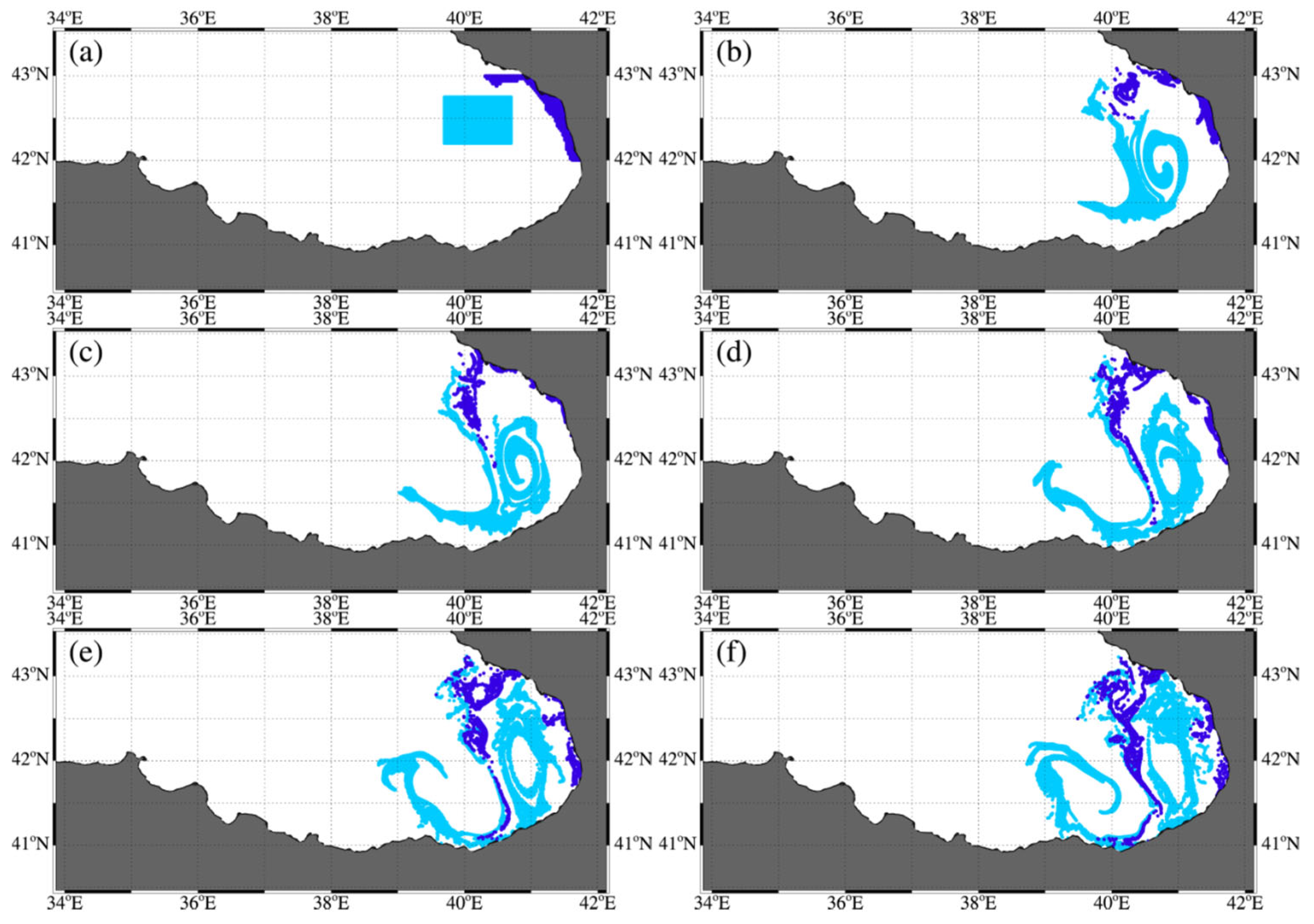
2.3. Lagrangian Particle Tracking

To complement the cross-shelf transport analysis facilitated by the assessment of the satellite and model generated data, a first-order accurate Lagrangian particle tracking scheme was applied to the NEMO model output. The transport pathways of particles released in the coastal regions of the south-eastern Black Sea, defined by depths less than 200 m, were calculated from the model simulated circulation fields at a 10 m depth. Such a high cut-off depth was chosen because the continental shelf is very steep in the eastern Black Sea. The scheme calculates the position of each drifter in time ( d x d t ) by integrating
d x d t = u ( x , t )
where the right-hand side is estimated with a Euler step forward in time (t) and space (x) using the daily velocity fields (u) at a 10 m depth. This scheme was chosen because it is simple and computationally efficient, and the choice of a very small time step (dt = 1 min) makes it comparable to a second-order accurate scheme ensuring appropriate accuracy. It is known that sub-grid scale dispersion processes that cannot be resolved by the discrete velocity fields, influence particle trajectories. In this study they were included in the particle tracking algorithms by superimposing a random walk term for each particle and time step [60,61] by using a Gaussian random process that resulted in an ~105 cm2s−1 diffusivity coefficient. In this study, we investigated an anticyclonic eddy in 1998 and a cyclonic eddy in 2000 in detail. Hence, two separate particle simulations were performed using the NEMO simulated circulation field of these years.

2.4. Cross-Shelf Volume Transport Calculations

The temporal evolution of cross-shelf transport is obtained by integrating cross-shelf volume fluxes in the water column. First, the shelf-break is defined on the model grid by selecting grid points corresponding to the enclosed 200 m contour (Figure 1).
Cross-shelf fluxes are obtained by projecting the simulated velocity fields orthogonal to the 200 m contour at each time step and depth. Off-shelf (on-shelf) volume transport is obtained by integrating the off-shelf (on-shelf) fluxes through the water column, which are then integrated for all of the grid points along the shelf boundary to obtain the basin-wide cross-shelf volume transport. Daily net volume transport across the shelf-break is the sum of the on-shelf and off-shelf volume transports (Equation (5)):
V T z 1 , z 2 o f f s h e l f = l 1 l 2 z 1 z 2 ( U . n ) d z   d l                   i f   U . n > 0
V T z 1 , z 2 o n s h e l f = l 1 l 2 z 1 z 2 ( U . n ) d z   d l                   i f   U . n < 0  
V T z 1 , z 2 N E T = V T z 1 , z 2 o f f s h e l f + V T z 1 , z 2 o n s h e l f
where V T z 1 , z 2 o f f s h e l f and V T z 1 , z 2 o n s h e l f represent the off-shelf and on-shelf volume transport, respectively. Integration is conducted between the depths of z 1 and z 2 , and between the start and end points ( l 1 and l 2 ) of the enclosed shelf-break boundary (200 m contour). U is the velocity vector on the shelf-break and n is the unit vector pointing off-shelf and normal to the shelf-break. Positive (negative) values represent off-shelf (on-shelf) transport. All cross-shelf transports presented (Section 3.3) in this paper are the net cross-shelf transport (Equation (5)) unless stated specifically as on-shelf/off-shelf. Total water column transport is calculated by integrating the whole water column from the surface to 200 m. “Surface transport” is defined as the transport calculated in the upper 50 m. “Deep layer transport” refers to the transport below the surface, that is, the transport calculated by integrating fluxes between 50 m and 200 m. All transports presented in Section 3.3 refer to the total water column (0–200 m) transport, except for figure in Section 3.3.1, which provides the cross-shelf exchanges at the surface and deep layers of the Black Sea. Annual climatologies of the cross-shelf transports were calculated from the daily time series for 1998–2014.
In order to estimate the eddy-induced transport, a filtered dataset was created from the simulations, where the modelled current velocities were filtered with a Hanning window (window size of 50 km) for each vertical layer and time step to obtain “large-scale” (larger than 50 km) circulation. The difference between the original and filtered current velocities is considered as the mesoscale circulation and is called the “eddy-induced” field. “Eddy-induced” cross-shelf transport is calculated using Equations (3)–(5), where U is replaced by the “eddy-induced” current velocity. Eddy-induced cross-shelf transport is divided by the total cross-shelf transport to obtain the percentage of eddy-induced transport.

3. Results

Mesoscale eddies and filaments were observed throughout the study period, both in the satellite images and model simulations. Features leading to cross-shelf exchange were found to belong to one of three groups: single eddies, eddy-dipoles, and eddy-filament pairs. However, it is often difficult to track these features in time on satellite images due to cloud contamination. We have identified numerous such cases, but it is difficult to assess the lifetime of these features due to inconsistent data availability. Therefore, here, we selected two cases in the south-east Black Sea: one along the Turkish coast and one along the Georgian coast, which were both visible for at least two consecutive weeks in the satellite images.

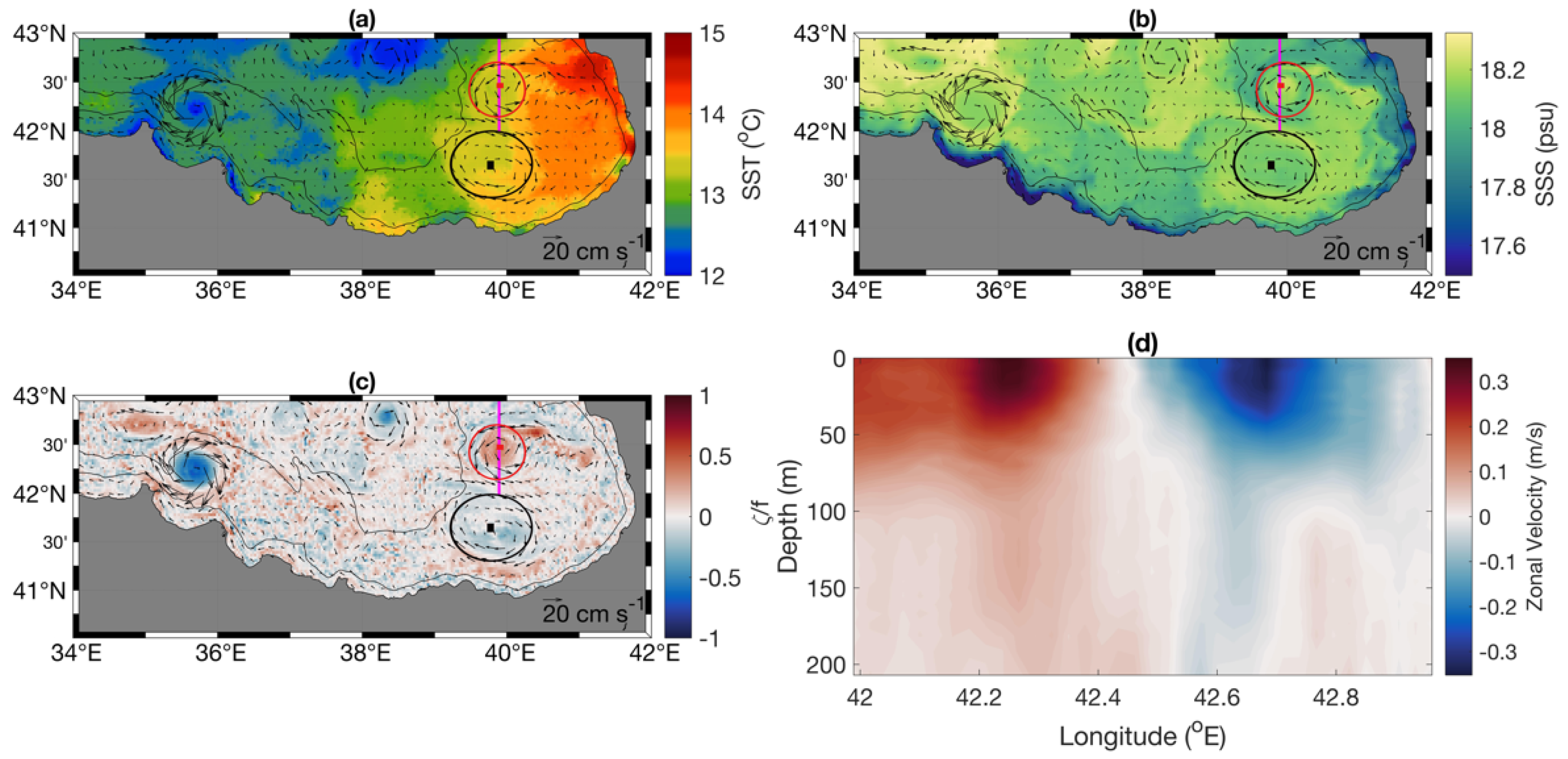
3.1. Anticyclonic Eddy along the Turkish Coast

In June 1998, Chl-a rich filaments were observed along the coast, from 35°E to 40°E. These Chl-a rich filaments were accompanied by mesoscale anticyclonic eddies (indicated by red circles, Figure 2). These features were observed as early as 23 April 1998, but due to cloud contamination, their continuity could not be confirmed. Filaments and associated eddies were observed for ~6 weeks starting on 21 May 1998 and continuing until 1 July 1998. During this period, Chl-a rich waters (1 mg/m3 and above) were carried offshore by the filament/eddy pairs (Figure 2).
At least three such filament/eddy features were observed; one located around 36°E–37°E (Figure 2), one around 38°E, and one around 39°E–40°E. The temporal evolution of cross-shelf chlorophyll concentration was demonstrated in a Hovmöller diagram showing a latitude mean (41.2°N–41.6°N, Figure 2a) between 38°E and 40°E (Figure 3a). High Chl-a values, typical of coastal waters, were observed between 39°E and 39.5°E, starting from 5 June 1998 and extended until 1 July 1998. Another patch of high Chl-a waters was observed at 38°E. Due to cloud coverage in satellite data in late April and the first two weeks of May, it is difficult to assess the exact start date of these filaments.
Imprints of these features were also observed in the satellite SST maps (Figure 4), where cold water patches were observed on 10 June 1998, extending offshore along the coastline, and on 11 June 1998 as a cold-water filament at 39.5°E. Eddies along the Turkish coast were also evident in the altimetry derived geostrophic velocity maps (Figure 5). A coastal anticyclone was seen on 10 May 1998 (Figure 5a) centred around 41.2°N and 40°E. Geostrophic currents pointed offshore on the western periphery of the anticyclonic eddy. This eddy moved further east until the end of May. By the end of May (Figure 5b), offshore directed currents could clearly be seen, and the cross-shelf transport was enhanced by an adjacent cyclone. On 14 June 1998, the anticyclonic eddy elongated into an eclipse (Figure 5c), and its location and size matched the satellite Chl-a observations (Figure 4b). The eddy was still persistent by the end of June (Figure 5d), transporting coastal waters offshore as evidenced by satellite Chl-a maps (Figure 2d).
To further investigate the fate of the filament/eddy features identified in the satellite data and assess the transport facilitated by them, model simulation was used. The major features seen in the satellite observations of Chl-a were also seen in the simulation results for the same period, making the model a tool to further explore the dynamics of cross-shelf circulation. While both filaments and eddies were spatially slightly displaced in the model simulation compared to the satellite observations, the size, rotation (cyclone vs. anticyclone), and positions generally agreed with the satellite observations (Figure 4).
An anticyclonic eddy was simulated (Figure 6) slightly east of Cape Sinop and propagated eastward toward Arkhangelsky ridge. Another anticyclonic eddy was simulated around 39°E with an associated filament, which was investigated in detail. Herein, this anticyclonic eddy will be referred to as AE1998. The filament associated with AE1998 intensified starting from 22 May 1998, and decelerated on 30 May 1998. The eddy lived on after the dissipation of the first filament, and a second filament formed on 4 June 1998. This filament was then observed in the simulations throughout June 1998. Starting on 16 June 1998, the eddy propagated northward, reducing the intensity of the filament, which eventually disappeared in the first week of July. Starting with the dissipation of the filament, the eddy no longer had an interaction with the shelf. The eddy was present in the simulations until the end of July 1998. However, cross-shelf transport was only facilitated between 22 May 1998 and 1 July 1998 (~40 days) until it moved further offshore into the deep basin.
Imprints of the filaments were also identified through the cross-shelf transport of low-salinity waters, which are typical of shelf waters subject to river discharge, which can be seen in the model simulated salinity fields (Figure 3b). The latitudinally averaged (41.2°N–41.6°N) salinity distribution in the study region showed that low salinity waters were observed around 39°E and transported offshore by the first filament observed between 22 May and 26 May 1998. Low salinity waters were then observed around 38.8°E (Figure 3b), starting on 4 June 1998, which corresponded to the second filament that was associated with the eddy.
The eddy–filament pair centred at 39°E appeared to have a relatively colder SST (~0.6 °C), compared to the surrounding, with temperatures similar to coastal waters (Figure 6a). Simulated surface salinity, on the other hand, showed the transport of low salinity (SSS <18 psu) waters along the filament (Figure 6b). The current velocity of the filament is equivalent to the angular velocity of the eddy, which is 0.3 m/s (Figure 6c). Below 120 m, eddy angular velocity is reduced to 0.1 m/s and less (Figure 6d).
This is supported by the Rossby numbers (i.e., relative vorticity normalised by planetary vorticity) of Ro = 0.5 that characterize the eddy. Negative vorticity of the eddy was accompanied by a positive vorticity (Ro = 0.3) on the north-west of the eddy (~42°N, 38.7°E), at the northernmost extension of the filament (Figure 6c). This cyclonic/anticyclonic flow separation (Figure 6c) transports low salinity waters further northwest (Figure 6b).
A detailed analysis of the satellite and model ADT data was carried out to investigate the characteristics of the AE1998 by applying the eddy detection and tracking algorithm described in Section 2.1 including the eddy amplitude, intensity, surface area, and radius. For this purpose, the mean eddy properties over the eddy lifetime of the anticyclonic eddy AE1998 were investigated (Table 1) and show that the mean values for amplitude, intensity, surface area, and radius obtained from the satellite ADT data were 3.20 cm, 28.28, 7.94 km2, and 46.75 km, respectively. Analysis of the model SSH field using the same algorithm showed that the amplitude, intensity, surface area, and radius of AE1998 was 6.68 cm, 29.44 and 9.65 km2, and 54.87 km, respectively. The differences between both analyses are likely to occur because the satellite ADT has a resolution of 13.78 km while the model resolution is 3 km.
The volume transported by the eddy can be estimated using the outputs of the eddy tracking algorithm by summation of the daily volume over the lifetime of the eddy. During its lifetime of 3 months, the eddy transported a total volume of 1.95 × 10⁸ Sv, with a daily mean volume transport of 2.17 × 10⁶ Sv. In that time, the eddy interacted with the shelf for only 40 days (22 May 1998–1 July 1998). Therefore, the volume transport via the eddy over 40 days was ~8.68 × 10⁷ Sv. These calculations give the cross-shelf transport if the eddy traps coastal waters and moves them off-shelf. However, for most of their lifetimes, eddies transport coastal waters on one side, via the filament. Hence, here we introduce a second estimation (Equation (1)), specifically to address this transport. The filament had a depth of ~130 m and a width of ~11 km, and an average velocity of 0.3 m/s at its core. Hence the filament transport was ~0.4 Sv per day.
To further investigate the effect of the eddy on the cross-shelf transport in the anticyclonic eddy, the Lagrangian drifter approach was employed as detailed above. In the case of the 1998 anticyclonic eddy, two sets of virtual particles were released and advected in the NEMO simulated circulation field in order to better illustrate the exchange between the shelf and the surrounding offshore waters (Figure 7a). A first set of 18,000 particles arose deployed on the continental shelf south of the anticyclonic eddy (Figure 7a, dark blue dots), and another set of 46,000 particles inside the anticyclone itself (light blue dots). Both sets of particles were launched on 13 June 1998 when the anticyclone was well-developed and the particles were tracked over 30 days. During the first 10 days of the simulation (Figure 7b, light blue), the particles deployed in the eddy stayed near the eddy centre and moved slightly eastward, a motion that was more obvious after 15 days (Figure 7c, light blue) when the drifters also moved closer to the shelf. Over time offshore filaments towards the northwest and northeast become apparent and 87.5% of the offshore particles stay offshore and only 12.5% get transported to the shelf (Figure 7, light blue). At the same time, the particles released on the shelf experience a strong offshore movement (Figure 7b, dark blue) that is associated with the filament described above and start rotating within the eddy (Figure 7c, dark blue), which becomes more evident over the course of the simulation and returns some of the initially offshore advected particles back toward the shore over the 30 day simulation (Figure 7f, dark blue). Some particles starting at the easternmost shelf were transported along the eastern and later north-eastern shelf areas (Figure 7, dark blue). Over the course of the simulation, 59% of the particles released on the shelf were transported offshore by the observed eddy/filament pair, 24% were transported to shelf areas to the east with a coastal current, and 17% remained in the release area. The offshore transport was mainly facilitated by the observed eddy/filament pair discussed above and after 30 days, the eddy transported 3% of the off-shore transported particles back to the release shelf area, which confirms the above results. The filament is the main off-shore transport mechanism with 0.4 Sv per day, while the rotating eddy itself also facilitates some onshore transport, however, that was much weaker compared to the offshore component.

3.2. Cyclonic Eddy along the Georgian Coast

The southeast Black Sea, particularly the Batumi area, is typically occupied by anticyclonic eddies, in both satellite observations and our simulations. To be able to investigate the dynamics of cross-shelf transport in a cyclonic eddy, here, we selected a rare cyclonic eddy.
In May 2000, a cyclonic eddy was observed in the satellite Chl-a images (Figure 8), centred around 41°E, ~41.7°N. An anticyclonic eddy was observed simultaneously at 39.8°E, 41.5°N, forming an eddy dipole. Imprints of this eddy dipole are filaments of high Chl-a waters. The anticyclonic eddy and associated filament were identified in three consecutive weekly satellite Chl-a images, whereas the cyclonic eddy and associated filaments were observed for five consecutive weeks. Satellite images suggest that the cyclonic eddy and associated filament formed on 6 May 2000, intensified by the end of May, and eventually disappeared in the last week of June 2000.
The time evolution of cross-shelf transport was demonstrated in a Hovmöller diagram showing a longitude mean (39.5°E–40.5°E, Figure 8a) between 41.5°N and 43°N (Figure 9a). High Chl-a values were observed between 39°E and 39.5°E, with peak values around 15 May 2000. After 10 June 2000, high Chl-a values were reduced, indicating the reduced cross-shelf (westward) transport of coastal waters.
Eddies observed via satellite Chl-a images were also seen in the altimetry derived geostrophic velocity maps (Figure 10). A cyclone and anticyclone dipole were observed on 10 May 2000 (Figure 10a), both centred around 41.5°N. Geostrophic velocity was directed offshore along the northern periphery of the cyclonic eddy (Figure 10). An anticyclone was present north of the cyclonic eddy starting on 23 June 2000 (Figure 10d), contributing to the offshore transport.
Model outputs were used to further investigate the cyclonic eddy identified in the satellite images and to quantify the transport facilitated by the eddy. The model successfully simulated the cyclonic eddy and its progression as well as the associated offshore transport of freshwater, enabling further investigation of the cross-shelf circulation dynamics. While the eddy in the simulation was spatially slightly displaced compared to the satellite observations, its size, rotation, and position agreed with the satellite observations (Figure 8). Herein, this cyclonic eddy is referred to as CE2000.
The cyclonic eddy was present in the simulations, starting from 1 April 2000 with a centre around 42°N–40.5°E (Figure 11 and Figure 12). The cyclonic eddy moved along the Rim Current northwards, reaching 42.25°N by 20 April 2000. It was present in this area (around 42.25°N–40.3°E) until end of May 2000, and then started to move southeast. During its move southeast, the eddy continuously transported coastal waters offshore (Figure 11), freshening the entire area between 40.2°E–42°E and 41.5°N–43°N, until it eventually dissipated in the first week of July.
Starting in the first week of May, low salinity waters, typical of shelf waters, were transported offshore by the eddy. Cross-shelf transport of low salinity waters reached a maximum by 15 May 2000, when the filament intensified, as observed by the freshening in the Hovmöller diagram (Figure 9b). Starting on 15 May 2000, low salinity waters (18 psu and lower) were observed, which was 0.2 psu fresher than previous values, indicating their coastal origin. On 25 May, mean salinity values showed even fresher (17.9 psu and below) waters, observed around 42.6°N. Similar mean salinity values were again observed in the same area between 6 June 2000 and 13 June 2000 (Figure 9b). After this date, a freshening was observed on the northern boundary of the area. These low salinity intrusions are the imprints of the shelf waters under river influence, transported offshore by the eddy and its associated filament in the area. In addition to the observed low-salinity intrusions, an overall freshening by ~0.2 psu was also evident in the Hovmöller diagram (Figure 9b), indicating that continuous cross-shelf transport by the eddy reduced the salinity in this area. The simulated progress of CE2000, the consequent advection of freshwaters, and eventually the reduction in the salinity of the entire area (40.2°E–42°E and 41.5°N–43°N) can be seen in Figure 11.
The eddy–filament pair centred at 42°N appears to have a colder SST (~0.5 °C) compared to the waters advected by the filament, with temperatures similar to coastal waters (Figure 12a). The SST distribution was difficult to assess as it also displayed a typical east–west SST gradient, with warmer waters on the east. Surface salinity (Figure 12b) on the other hand, clearly showed the transport of low salinity (SSS < 18 psu) waters along the filament. Current velocity of the filament was equivalent to the angular velocity of the eddy, which was 0.3 m/s (Figure 12). Below 80 m, the eddy angular velocity was reduced to 0.1 m/s and less. The eddy was characterised by Rossby numbers of Ro = 0.4 (Figure 12c).
Characteristics of the CE2000 detected and tracked by the EddyScan over its lifetime using the satellite ADT and model ADT data showed that CE2000 detected from the satellite had an amplitude of 2.04 cm, intensity of 17.76, surface area of 6.32 km2, and a radius of 41.91 km on average over its lifetime (Table 2). The CE2000 detected from the model SSH simulation had an amplitude of 5.63 cm, intensity of 13.80, surface area of 5.14 km2, and radius of 38.30 km.
The volume of water transported by this eddy was estimated for 40 days, over which the eddy tracking algorithm detected this eddy. The eddy facilitated a total volume transport of 8.6 × 10⁷ Sv over this time, with a daily mean of 2.2 × 10⁶ Sv. These calculations can provide cross-shelf transport, if the eddy traps the coastal waters and moves them off-shelf. However, that was not the case, and the eddy transported coastal waters only on one side via the filament. Here, the filament had a depth of ~80 m and a width of ~18 km, and an average velocity of 0.3 m/s at its core. Hence, the filament transport was ~0.4 Sv per day. Although CE2000 was shallow compared to the anticyclone (AE1998), transport via the filament was similar as the filament was wider.
As performed for the anticyclonic eddy, the effect of the cyclonic eddy on the cross-shelf transport in the cyclonic eddy was investigated with the Lagrangian drifter approach releasing virtual drifters on the north-eastern shelf and the surrounding, offshore waters of the eddy (Figure 13a). A first set of 10,000 particles was released over the eastern continental shelf adjacent to the simulated cyclonic eddy (Figure 13, dark blue dots) and at the same time 26,000 drifters, were released in the cyclone itself (light blue dots). Both sets of particles were launched on 15 May 2000 and tracked over 30 days. During the first 10 days of the simulation (Figure 13b, light blue), the particles deployed in the eddy moved rapidly southward following the tracks of the eddy, and then continued rotating within the moving eddy, staying in the area until day 25 of the simulation (Figure 13e, light blue) and then moving northward again by day 30 of the simulation (Figure 13f, light blue). Over time, eastward offshore filaments become apparent and some of the particles also reach the southern shelf. In total, 88% of the offshore particles stayed offshore and only 12% were transported to the southern shelf (Figure 13, light blue). At the same time, the particles released on the shelf experienced some offshore movement (Figure 13b, dark blue) and started moving southward within the eddy (Figure 13d, dark blue), which became more evident over the course of the simulation and moved some of the initially offshore advected particles back toward the southern shore over the 30 day simulation (Figure 13f, dark blue). Some particles starting at the southern part of the shelf were also transported southward on the shelf (Figure 13, dark blue). Over the course of the simulation, 27% of the particles released on the shelf were transported directly offshore by the observed eddy and the remaining 73% of the particles were found on the shelf. However, only 27% of all drifters were retained on the release shelf, the remaining drifters reached shelf areas away from their origin, transported first offshore, or in currents along the coast. In total, 46% of the drifters originating on the shelf were transported away from the area. Therefore, the off-shore transport by this very different eddy was less than the anticyclonic eddy with a similar volume transported by the filament associated with it.

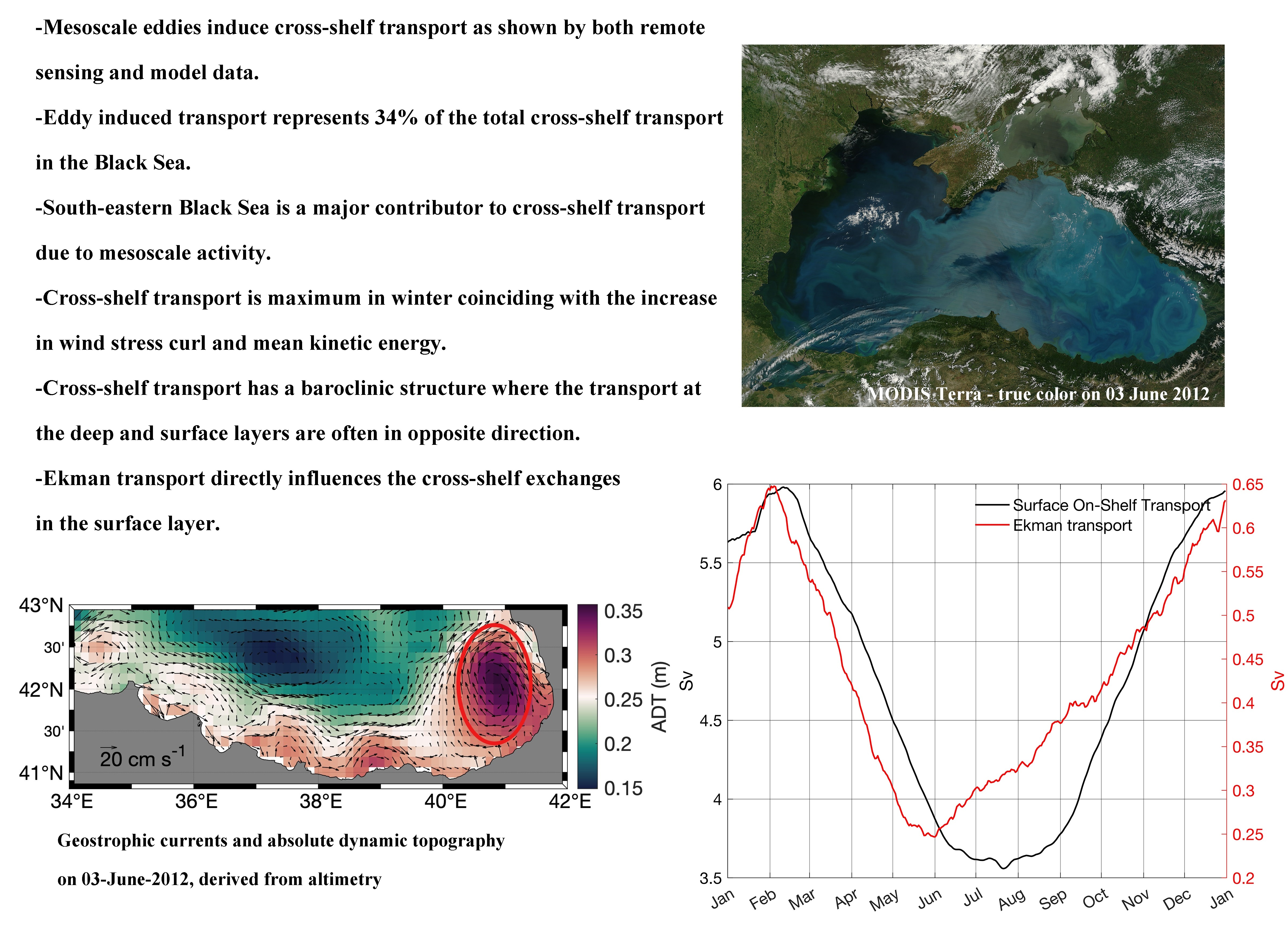
3.3. Cross-Shelf Exchanges

In this section, the temporal variability of the cross-shelf exchange in the Black Sea as a whole is investigated using the model simulation. The shelf-break is the main area for instabilities to occur due to topographic irregularities. In addition, this region is under the influence of river discharges, leading to baroclinic instability. Hence, both density forcing and topographic steering play an important role in the generation and modification of shelf-break eddies and filaments. Here, we again used the 200 m contour as representative of the shelf-break in the Black Sea. Cross-shelf exchanges were calculated as the net integrated volume transport across the closed 200 m contour.

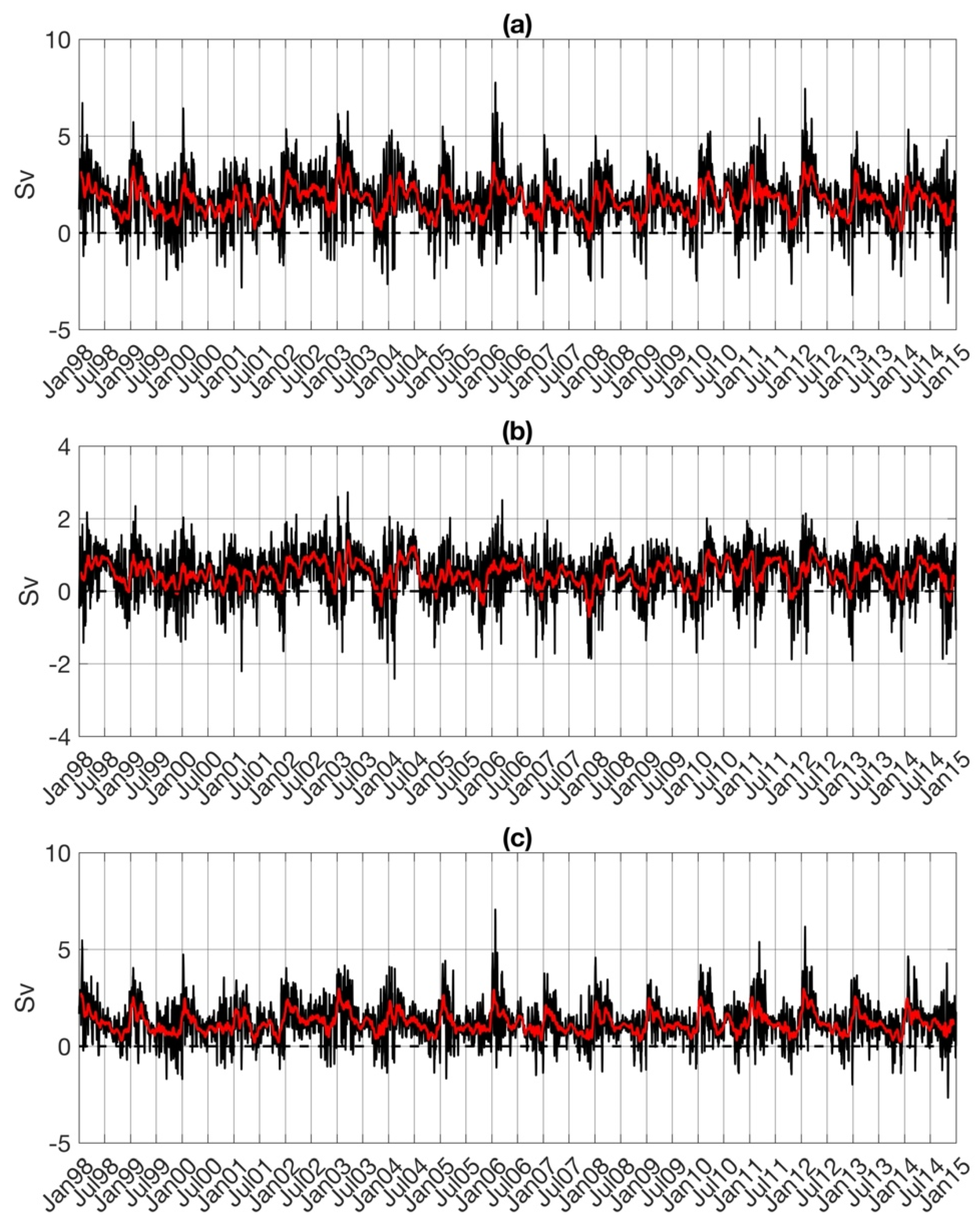
3.3.1. Cross-Shelf Exchanges in Black Sea

The daily, water column integrated, net transport across the shelf-break calculated for the entire Black Sea for the time frame January 1998 to December 2014 displayed a seasonal cycle with the maximum off-shelf transport in early winter and spring and the maximum on-shelf transport in autumn (Figure 14a). This seasonality existed for most of the time-series, but episodic transport events also existed such as the on-shelf (negative) transport peak in spring 2001 (Figure 14a).
Both off-shelf and on-shelf transport episodes were observed but the prevailing direction for transport was off-shelf. This clearly indicates that the shelf-break facilitates an important transport pathway; mainly carrying shelf waters to the deep basin, but at times also facilitating the transport of waters in the open sea onto the shelf (negative transports). Off-shelf transport is typically about 3 Sv, but the maxima can exceed 7 Sv. On-shelf transport is typically 1 Sv, but the transport maxima can exceed 3 Sv.
Although the net, water-column integrated transport across the shelf-break is mainly off-shelf, this water column has a baroclinic structure, where the transport at the surface and in deeper layers are often in the opposite direction. Here, we dissect the shelf-break transport as “surface (0–50 m)” and “deep layer (50–200 m)” transport (see Equations (3)–(5) and Section 2.4 for details) to show the variability in the wind-driven upper layer and isolated deep layers.
In the surface layer (Figure 14b), on-shelf transport was more frequently present than in the deep layer (Figure 14c) which was dominantly off-shelf. Overall, the surface transport (Figure 14b) was mainly off-shelf, but also displayed regular on-shelf transport periods. Transport at the deep layers (Figure 14c) is protected from the impact of winds, and hence abides topographic control, resulting in downslope (off-shelf) transport. This baroclinic structure arises from the fact that wind forcing plays a critical role in the upper layer of the Black Sea. Thus, the wind driven surface layer has a transport signal that is more chaotic (Figure 14b) compared to the transport at the deep layers (Figure 14c) or the whole water column integrated transport (0–200 m) (Figure 14a).

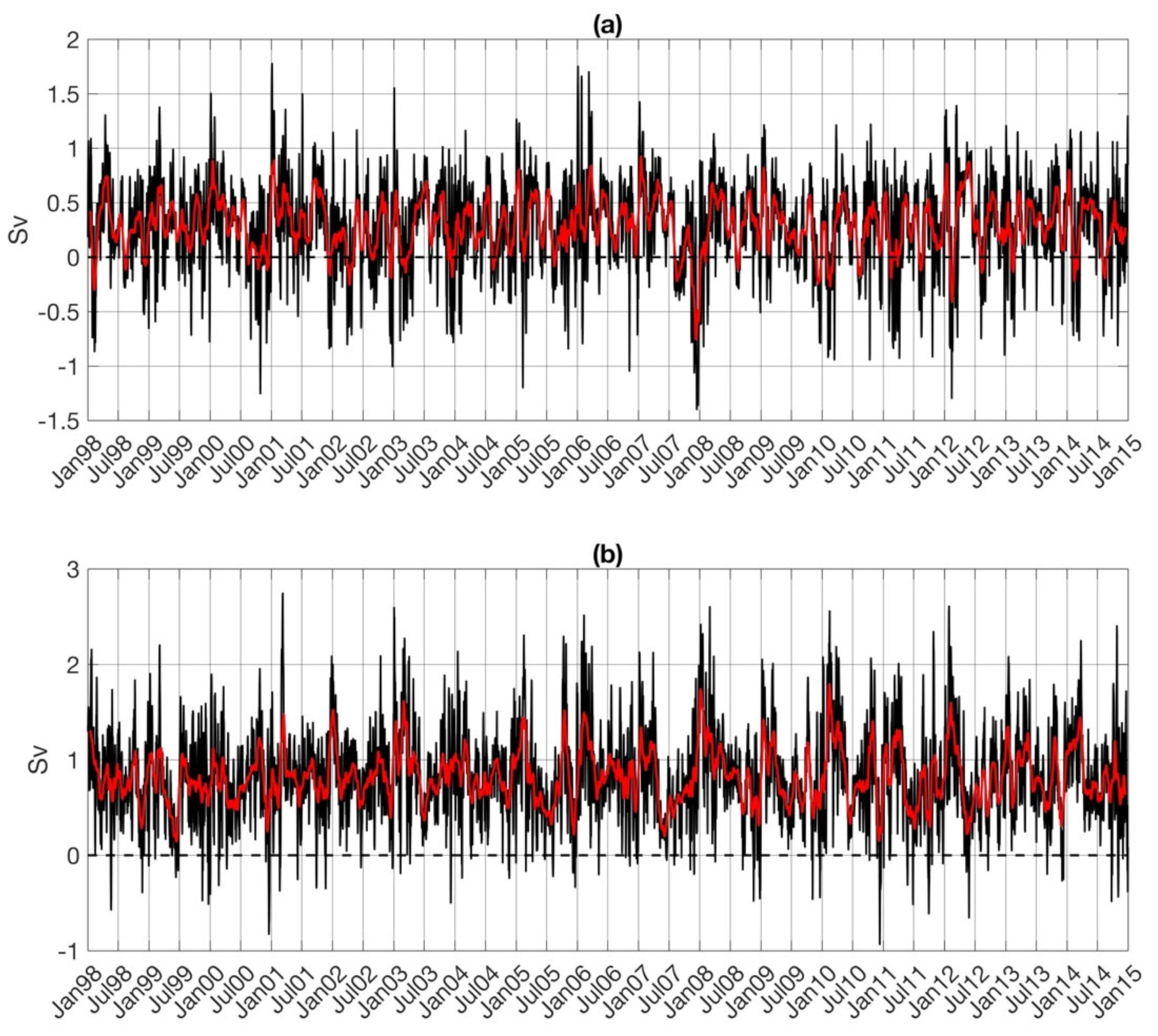
3.3.2. Cross-Shelf Exchanges in the South-East Black Sea

After looking at the variability of transport with depth, it is also necessary to look at spatial variability, as different regions may be dominated by different processes. In this section, we therefore present the cross-shelf transport in the south-eastern Black Sea, using a 500 km section (Figure 1, magenta section) of the shelf-break to assess the dynamics of the cross-shelf transport in this region.
Cross-shelf transport in the south-east Black Sea is dominantly off-shelf (Figure 15a). Transport is mostly off-shelf in winter, but there is no clear seasonality of the transport direction. Cross-shelf transport is typically less than 1 Sv in either direction, with an off-shelf transport maxima exceeding 1.5 Sv and an on-shelf transport maxima exceeding 1 Sv.
In order to assess the relative importance of the south-eastern Black Sea, we compared its cross-shelf transport with the north-western Black Sea using equal sections of 500 km for both (Figure 1, blue section). The north-western Black Sea was chosen for comparison, because it is an area known for strong cross-shelf transport [62,63] and also showed the strongest off-shelf transport signal in our analysis. Cross-shelf transport in the north-western Black Sea was dominantly off-shelf, with few occasions of on-shelf transport (Figure 15b). This is mainly due to the large freshwater input onto the north-western shelf [62]. Cross-shelf transport in the northwest was typically around 1–1.5 Sv (Figure 15b), whereas in the southeast Black Sea, it was around 0.5 Sv (Figure 15a).
Cross-shelf transport was typically two to three times lower in the south-eastern Black Sea compared to the north-western Black Sea (Figure 15b). Furthermore, the south-eastern Black Sea has many more occasions of on-shelf transport, whereas the north-western Black Sea is dominated by off-shelf transport. However, even though the magnitude of cross-shelf transport in the south-eastern Black Sea is only secondary to that of the north-western Black Sea, these results demonstrate that the south-eastern Black Sea is an important region for the cross-shelf export of coastal waters.

3.3.3. Seasonality of Cross-Shelf Exchanges

To further investigate the winter maxima of the cross-shelf exchanges presented in the previous section, seasonality was investigated in this section using annual climatologies. The water column (0–200 m) integrated cross-shelf exchange had a clear seasonal signal, where the maximum values were observed between January and March, with a gradual decline after March (Figure 16a). This confirms that although the cross-shelf exchange had high frequency variability (daily oscillations, Figure 14a), it also had a clear seasonal signal. The south-eastern Black Sea also had a winter maximum (Figure 16a), but an oscillating signal for the rest of the year.
The water column integrated (0–200 m) cross-shelf exchange correlated well (r = 0.59) with the basin averaged wind stress curl (Figure 16b). Seasonal signals had the highest correlation between January and October (r = 0.89).
In the surface layer (0–50 m), net transport was mostly off-shelf but regularly displayed on-shelf transport events (Figure 14b). Seasonally, net cross-shelf transport at the surface layer was negatively correlated (r = −0.57) with the Ekman transport. As the Ekman transport increased, the net surface cross-shelf transport was reduced, meaning that the Ekman transport increased the on-shelf transport. To verify this, we present the on-shelf surface (0–50 m) transport (Figure 17). Seasonally, the surface on-shelf transport was highly correlated with the Ekman transport (r = 0.9 with 5 days lag).

4. Discussion

4.1. Eddies in the South-Eastern Black Sea

An anticyclone near the Turkish coast (AE1998) and a cyclone near the Georgian coast (CE2000) were investigated in detail to estimate the eddy induced offshore transport in the area using satellite observations and models, capable of successfully simulating the Black Sea eddy dynamics [33]. These eddies were simulated in the model, but compared to the satellite observations, were slightly displaced in the simulations. However, the size, rotation (cyclone/anticyclone), and progress agreed with the satellite observations. Although the eddies observed by satellite data and the model were in good agreement, they were not identical. This is to be expected. Specifically, a cyclone was observed adjacent to AE1998 in the altimetry data (Figure 5b), which did not appear in the model.
The distribution of SST and SSS around the eddy/filament pair was similar to the shelf waters, indicating the transport of coastal waters by the eddies. For most of their lifetimes, the AE1998 and CE2000 were accompanied by cyclonic and anticyclonic wind stress curl, respectively (Figure 18). The area where AE1998 and the CE2000 occurred corresponded to the local wind stress curl features [45], which are the tip jets near Cape Fener and the Kolkheti Valley winds, respectively (see Figure 1). Hence, vorticity input by wind stress is an important contributor to eddies in the region. The analysis revealed that both of the presented eddies may be a result of freshwater influx and wind [36] because both cases occurred at a time of increased freshwater influx to the shelf. Ref. [48] also observed cyclonic wind stress curl to be the driver of cyclones (similar to CE2000) in the same (Batumi) area, coherent with our findings (Figure 18f–j). Such eddies were shown to dominate the Batumi area in winter [48], whereas a recent study also presented an eddy dipole, consisting of a cyclonic and an anticyclonic eddy in the area [42], similar to the eddy dipole presented here (CE2000). Although the size (~50 km) and location of the eddies presented by [42] are coherent with our findings, we present a case during the spring/summer transition. Hence, we show that cyclonic eddies may form in the Batumi area in different seasons, providing that the wind stress curl is cyclonic. An anticyclonic eddy was previously presented [42] in the same area as ours (AE1998). Our simulations suggest that the occurrence of such anticyclonic features in the area are often accompanied by an anticyclonic wind stress curl field (e.g., Figure 18a–e). AE1998 and CE2000 had sizes of ~50 km in agreement with previous findings of eddies with an ~50–60 km radius [42,48] in the area. The orbital velocity of AE1998 and CE2000 were found to be ~0.3 m/s on average, also in agreement with similar sized eddies observed in the area that had orbital velocities of ~0.2–0.3 m/s [8,42].
Eddy lifetime, eddy area, and the displacement of the eddy centre were obtained from the eddy-tracking algorithm and the horizontal volume transport of the eddies was estimated following [33,59] by multiplying the eddy area by the depth of the eddy, which was 130 m for AE1998 and 80 m for CE2000, respectively. However, the transport of the eddy often occurs on one side [23,34]. It is therefore an approximate estimate of the volume transported by the eddies. Furthermore, the EddyScan algorithm did not identify CE2000 during the early days of its lifetime as it could not detect a closed contour, even though the eddy could be seen in the vorticity distribution. This is the reason why its detected lifetime of ~40 days was much lower than that of the AE1998. However, regardless of the exact total lifetime, our estimations of the daily mean volume transport for both eddies were similar: 2.17 × 10⁶ Sv and 2.2 × 10⁶ Sv for AE1998 and CE2000, respectively. These estimates were of the same order of the transport magnitude as similar sized eddies of ~50 km radius in the north-western shelf [23,34]. The eddies presented here were accompanied by filaments for most of their lifetime, through which the main eddy transport occurred. The separately calculated filament transports were found to be ~0.4 Sv/day for both AE1998 and CE2000. It is difficult to assess the “exact” transport by these eddies, as they move on and off the shelf, and filaments appear and disappear during their lifetime. Therefore, we provided both the filament transport, and the approximate volume of the eddies.
The characteristics (i.e., eddy amplitude, intensity, surface area, and radius) of both AE1998 and CE2000 detected from model ADT were partly in agreement with the characteristics of AE1998 and CE2000 detected and tracked from the satellite ADT by applying EddyScan. However, the coarser resolution of the satellite ADT data (13.78 km) and the lower quality of altimetry data in coastal areas resulted in an inevitable difference between the characteristics of the detected eddies. Nevertheless, the surface area and radius of both AE1998 and CE2000 obtained from the satellite data and model simulation were in close agreement, indicating that the model represents the Black Sea dynamics well.
The Lagrangian drifter simulation results support the observation that both eddies facilitate offshore transport, though the simulations revealed a remarkable difference between the two eddies in the number of particles exported offshore by the surface flow. CE2000 exported 27% of the particles released on the shelf directly offshore and another 19% of the particles to shelf areas located south of the release area. This was due to the eddy moving offshore and southward early on in the simulation time period. AE 1998 exported 59% of the particles released on the shelf to offshore with only 17% of the particles remaining on the shelf.

4.2. Cross-Shelf Exchanges in the Black Sea

Our comparisons of integrated net cross-shelf transport across the 500 km section along the south-eastern Black Sea shelf (Figure 15a) were often half that of a similar 500 km section along the north-western Black Sea shelf (Figure 15b), which is the most important area of cross-shelf transport in the Black Sea, which is associated with its large freshwater influx and associated instabilities [62,63]. Hence, we concluded that the south-eastern Black Sea is an important pathway for the cross-shelf transport of materials and biota. We speculate that this mechanism also supports carbon export from the productive shelf to the deep basin, hence acting as a sink mechanism for atmospheric carbon. A recent study has also shown the importance of cross-shelf buoyancy fluxes on the generation of submesoscale eddies in the Black Sea [64], which likely has further implications for biogeochemistry.
Over the same study period of 1998 to 2014, the along-shelf transport (not shown), which represents the flow of the Rim Current, was ten to twenty times more than the cross-shelf transports presented in Section 3.3. The cross-shelf transport is therefore only of secondary importance compared to the along-shelf transport, as expected due to the nature of cross-shelf flows [18]. To our knowledge, only [21] has provided a comparison of the cross-shelf vs. along-shelf currents and have found the along-shelf currents to be 5–10 times, with some instances of 25 times that of the cross-shelf currents. Hence, our ratio of 0.05 to 0.1 was slightly less than theirs, but of similar magnitude.
Cross-shelf transport has a seasonal signal (Figure 14a), displaying the maxima in winter when the intensity of the cyclonic circulation (i.e., mean kinetic energy—MKE) is increased. Cross-shelf transport in the Black Sea has a pronounced seasonality (Figure 16a), which correlates well with the wind stress curl (Figure 16b, r = 0.59) and is closely coupled between January and October (r = 0.89). Cross-shelf transport in the south-eastern Black Sea also showed the maxima in winter (Figure 16a), but did not have a distinctive seasonal cycle that could be linked to a forcing mechanism. This was most probably caused by the nature of our calculations. Cross-shelf exchanges were calculated on an open boundary (magenta line, Figure 1), which prevented clear seasonal signals because the budget was not closed.
Variability in the cross-shelf transport has been found to be correlated with the mean kinetic energy (r = 0.55) interannually, which itself is closely correlated (r = 0.84) with the basin-averaged wind stress curl. In other words, cross-shelf transport extrema were observed in winter, closely linked to the intensity of overall circulation (i.e., mean kinetic energy), which is correlated to the wind stress curl. In winter, as the wind forcing is increased, Black Sea cyclonic circulation intensifies [10], leading to intensified coastal downwelling (i.e., anticyclonic circulation) [65]. The eddy activity is reduced [13]; however, eddies are energetic [33], contributing to cross-shelf transport [42].
The increase in cross-shelf (i.e., off-shelf) transport during winter can be linked to the boundary current intensity itself. As the boundary current is intense in winter, any violation of the Taylor–Proudman assumptions will lead to intense cross-shelf transport. In particular, Ekman transport is due to strong winds and eddy-induced transport through energetic eddies at the surface, whereas in the bottom, influenced by a bottom boundary layer (i.e., the bottom Ekman layer) in the boundary, the current may be subject to cross-shelf transport, depending on the friction and topographic slope, namely “Ekman drainage” [66,67], further contributing to the off-shelf transport (Figure 14). This mechanism was also observed in the Black Sea. Particularly in the presence of an intense boundary current such as occurs in winter, a bottom boundary layer is formed where the Ekman water transport is perpendicular to the current [21]. The thickness of this layer has been correlated with the current velocity in its upper boundary [68]. Transport of the bottom boundary layer has also been suggested as a ventilation mechanism of the pycnocline [69,70]. Another reason for the cross-shelf transport maxima in winter may be the density gradients. Shelf waters become denser in winter due to convection, which may lead to a cascading of dense waters down the continental slope [67]. Both the Ekman drainage and dense-water cascading are directly influenced by the friction and topographic slope.
In this study, the upper 50 m layer was selected to represent the surface layer under wind influence, corresponding to the average estimation of a mixed layer depth, which was 40–45 m at the periphery of the basin [71]. The cross-shelf transport at the surface (0–50 m) was under the direct influence of the wind (i.e., Ekman transport) as well as the eddy activity. Seasonally, on-shelf transport at the surface (0–50 m) was well-correlated (r = 0.9) with a lag of 5 days to Ekman transport. This is in agreement with the fact that as wind stress curl (and Ekman pumping) increases, open-waters are carried to the coast by Ekman transport [13]. The response time of 5 days was low compared to the previous estimate of ~14 days required to carry waters from the centre to coast (basin radius ~200 km). This may be is a consequence of using Ekman transport projected onto the shelf-break (Figure 1). Hence, our results of a 5-day lag represent the time to just cross the shelf-break and not carrying waters across the basin.
However, it is difficult to differentiate between the surface Ekman transport and eddy induced transport signals as they often co-exist. The surface and bottom Ekman transport, dense water cascading, and eddies are the potential causes of cross-shelf transport in the Black Sea. However, in order to assess the relative contribution of these mechanisms, control simulations with which the effects of wind, topography, and freshwater influence can be tested are required.
One main outcome of this study was the estimation of eddy-induced cross shelf exchanges, which were estimated for individual eddies. However, it is difficult to assess the total eddy-induced cross-shelf exchanges over time in the whole Black Sea, especially for individual eddies on the shelf-break, whose on-shelf/off-shelf transports often negate each other. In order to provide an estimate of the eddy transport, here, we used the “eddy-induced” circulation fields (see Section 2). Both large-scale transport (Figure 19a) and eddy-induced (i.e., mesoscale) transport (Figure 19b) had a maxima in winter, similar to the total transport (Figure 14a). Eddy-induced transport also had a high intra-seasonal (sub-monthly) variability. Seasonally (Figure 19c), large-scale transport showed a decline after winter. Eddy-induced transport had a major increase in May–July, consistent with increasing the summer-time eddy activity [27]. However, the eddy-induced transport was still the maximum in winter.
Eddy-induced off-shelf transport is responsible for 34% of the total off-shelf transport in the Black Sea. Similarly, eddy-induced on-shelf transport is responsible for 37% of the total on-shelf transport in the Black Sea. The percentage of eddy-induced across-shelf transports changes between 25 and 65% over time (Figure 20). Our definition of the “eddy-induced” transport is likely to be subject to errors as we filtered the model fields with a 50 km Hanning window and then subtracted it from the original simulated fields. It is therefore likely that these results do not account for eddies larger than 50 km. However, it is an efficient way to represent the “mesoscale” or “eddy-induced” cross-shelf transport.
In this study, we provided an overview of cross-shelf transports, with a particular focus on the eddy-induced cross-shelf transport. However, as mentioned previously, our representation was limited to mesoscale eddies. The Black Sea, particularly the shelf-break, is an area of submesoscale eddies [36,38], with implications for cross-shelf transport [39]. Assuming that models can effectively reproduce features with ~7 times of their horizontal resolution [72], models with a horizontal resolution of ~1 km and below are required to effectively resolve submesoscale eddies. A comparison of models with low and high horizontal resolution [73,74] have shown the necessity of high-resolution simulations to capture the cross-shelf exchanges due to submesoscales. Particularly, over the shelf-break, the Rossby radius of deformation changes rapidly, hence high-resolution simulations are necessary to represent cross-shelf exchanges at submesoscales. Alternatively, adaptive horizontal resolution could be used with increased resolution at the shelf-break [75].

5. Conclusions

Cross-shelf exchanges were investigated using remote sensing data and an ocean circulation model to which an eddy-tracking algorithm and Lagrangian particle tracking model were applied. In the south-eastern Black Sea, an anticyclonic eddy (AE1998) and a cyclonic eddy (CE2000) with associated filaments have been identified in the remote sensing data. Both eddies transported high Chl-a waters associated with low salinities, typical of shelf origin, offshore. Size and angular velocity of these eddies were compatible with earlier findings in the region. Cross-shelf transport by AE1998 and CE2000 were coherent with similarly sized eddies in the north-western shelf. Particle tracking results confirmed that both eddies transported coastal waters offshore with the main transport facilitated by filaments associated with each eddy.
The net water-column integrated transport across the shelf-break of the Black Sea was investigated for the time frame 1998–2014 and was found to be mainly off-shelf, with the water column having a baroclinic structure, where the transport at the surface (0–50 m) and in deeper layers (50–200 m) are often in the opposite direction. We observed a cross-shelf transport maxima in winter, closely linked to the intensity of cyclonic circulation, which correlated to the wind stress curl inter-annually. As the wind forcing increased during winter, the cyclonic circulation of the Black Sea intensified, and the Ekman transport then pushed open-waters to the coast, promoting intensified coastal anticyclonic circulation. At the same time, a bottom Ekman boundary layer was observed and downwelling circulation (off-shelf transport) was intensified. Although the number of eddies was reduced in that season, the remaining eddies were energetic and contributed to the cross-shelf transport. Mesoscale eddies were responsible for 34% of the total off-shelf transport and 37% of the on-shelf transport.
The relative importance of the south-eastern Black Sea was investigated by comparing its cross-shelf exchange magnitude with that of the north-western shelf, which is a known area of major river discharges as well as the cross-shelf exchange. The south-eastern Black Sea is only secondary to the north-western shelf in terms of the cross-shelf exchange magnitude, but the results showed that it is an area of net off-shelf transport. We conclude that the south-eastern Black Sea is an important pathway for the cross-shelf transport of materials and biota. We speculate that this mechanism also supports carbon export from the productive shelf to the deep basin, hence acting as a sink mechanism for atmospheric carbon. Simulations with higher spatial resolution are required to investigate the contribution of submesoscale processes to the mesoscale processes provided here.

Author Contributions

Conceptualisation, A.A. and E.S.; Methodology, A.A., E.S. and B.A.F.; Software, E.S., B.A.F. and S.A.; Validation, A.A., E.S., B.A.F. and S.A.; Formal analysis, A.A., E.S. and B.A.F.; Investigation, A.A. and E.S.; Resources, E.S., B.A.F. and S.A.; Data curation, A.A. and E.S.; Writing—original draft preparation, A.A. and B.A.F.; Writing—review and editing, E.S. and S.A.; Visualisation, A.A., E.S. and B.A.F. All authors have read and agreed to the published version of the manuscript.

Funding

This research was partially supported by 118Y424 project of the Turkish Scientific and Technical Council (TÜBITAK) and the EU H2020 project DOORS (contract no. 101000518). The authors also acknowledge the support by DEKOSIM (BAP-08-11-DPT2012K120880) funded by the Turkish Ministry of Development. Anıl Akpınar acknowledges support by the TUBITAK 2211-C Programme.

Data Availability Statement

The satellite datasets used in this work are publicly available online through the Copernicus Marine Environment Monitoring Service (CMEMS) project (https://resources.marine.copernicus.eu/product-detail/OCEANCOLOUR_BS_CHL_L3_REP_OBSERVATIONS_009_071/INFORMATION, accessed on 27 June 2022) and (https://resources.marine.copernicus.eu/product-detail/SST_BS_SST_L4_REP_OBSERVATIONS_010_022/INFORMATION, accessed on 27 June 2022). The model outputs used in this work can be found at https://doi.org/10.5281/zenodo.6778391.

Acknowledgments

This study was conducted using E.U. Copernicus Marine Service Information (CMEMS, https://marine.copernicus.eu/, accessed on 27 June 2022).

Conflicts of Interest

The authors declare no conflict of interest.

References

  1. Ginzburg, A.I.; Kostianoy, A.G.; Sheremet, N.A. Seasonal and Interannual Variability of the Black Sea Surface Temperature as Revealed from Satellite Data (1982–2000). J. Mar. Syst. 2004, 52, 33–50. [Google Scholar] [CrossRef]
  2. Sakalli, A.; Başusta, N. Sea Surface Temperature Change in the Black Sea under Climate Change: A Simulation of the Sea Surface Temperature up to 2100. Int. J. Climatol. 2018, 38, 4687–4698. [Google Scholar] [CrossRef]
  3. Mohamed, B.; Ibrahim, O.; Nagy, H. Sea Surface Temperature Variability and Marine Heatwaves in the Black Sea. Remote Sens. 2022, 14, 2383. [Google Scholar] [CrossRef]
  4. Capet, A.; Barth, A.; Beckers, J.-M.; Marilaure, G. Interannual Variability of Black Sea’s Hydrodynamics and Connection to Atmospheric Patterns. Deep Sea Res. Part II Top. Stud. Oceanogr. 2012, 77–80, 128–142. [Google Scholar] [CrossRef]
  5. Akpinar, A.; Fach, B.A.; Oguz, T. Observing the Subsurface Thermal Signature of the Black Sea Cold Intermediate Layer with Argo Profiling Floats. Deep Sea Res. Part Oceanogr. Res. Pap. 2017, 124, 140–152. [Google Scholar] [CrossRef]
  6. Miladinova, S.; Stips, A.; Garcia-Gorriz, E.; Macias Moy, D. Black S Ea Thermohaline Properties: Long-term Trends and Variations. J. Geophys. Res. Ocean. 2017, 122, 5624–5644. [Google Scholar] [CrossRef]
  7. Stanev, E.V.; Chtirkova, B. Interannual Change in Mode Waters: Case of the Black Sea. J. Geophys. Res. Ocean. 2021, 126. [Google Scholar] [CrossRef]
  8. Oguz, T.; Latun, V.S.; Latif, M.A.; Vladimirov, V.V.; Sur, H.I.; Markov, A.A.; Özsoy, E.; Kotovshchikov, B.B.; Eremeev, V.V.; Ünlüata, Ü. Circulation in the Surface and Intermediate Layers of the Black Sea. Deep Sea Res. Part Oceanogr. Res. Pap. 1993, 40, 1597–1612. [Google Scholar] [CrossRef]
  9. Korotaev, G. Seasonal, Interannual, and Mesoscale Variability of the Black Sea Upper Layer Circulation Derived from Altimeter Data. J. Geophys. Res. 2003, 108, 3122. [Google Scholar] [CrossRef]
  10. Stanev, E.V. On the Mechanisms of the Black Sea Circulation. Earth-Sci. Rev. 1990, 28, 285–319. [Google Scholar] [CrossRef]
  11. Grayek, S.; Stanev, E.V.; Kandilarov, R. On the Response of Black Sea Level to External Forcing: Altimeter Data and Numerical Modelling. Ocean Dyn. 2010, 60, 123–140. [Google Scholar] [CrossRef]
  12. Kubryakov, A.A.; Stanichny, S.V.; Volkov, D.L. Quantifying the Impact of Basin Dynamics on the Regional Sea Level Rise in the Black Sea. Ocean Sci. 2017, 13, 443–452. [Google Scholar] [CrossRef]
  13. Kubryakov, A.A.; Stanichny, S.V.; Zatsepin, A.G.; Kremenetskiy, V.V. Long-Term Variations of the Black Sea Dynamics and Their Impact on the Marine Ecosystem. J. Mar. Syst. 2016, 163, 80–94. [Google Scholar] [CrossRef]
  14. Miladinova, S.; Stips, A.; Macias Moy, D.; Garcia-Gorriz, E. Seasonal and Inter-Annual Variability of the Phytoplankton Dynamics in the Black Sea Inner Basin. Oceans 2020, 1, 251–273. [Google Scholar] [CrossRef]
  15. Cokacar, T.; Oguz, T.; Kubilay, N. Satellite-Detected Early Summer Coccolithophore Blooms and Their Interannual Variability in the Black Sea. Deep Sea Res. Part Oceanogr. Res. Pap. 2004, 51, 1017–1031. [Google Scholar] [CrossRef]
  16. Kubryakov, A.A.; Mikaelyan, A.S.; Stanichny, S.V. Summer and Winter Coccolithophore Blooms in the Black Sea and Their Impact on Production of Dissolved Organic Matter from Bio-Argo Data. J. Mar. Syst. 2019, 199, 103220. [Google Scholar] [CrossRef]
  17. Kubryakova, E.A.; Kubryakov, A.A.; Mikaelyan, A.S. Winter Coccolithophore Blooms in the Black Sea: Interannual Variability and Driving Factors. J. Mar. Syst. 2021, 213, 103461. [Google Scholar] [CrossRef]
  18. Brink, K.H. Cross-Shelf Exchange. Annu. Rev. Mar. Sci. 2016, 8, 59–78. [Google Scholar] [CrossRef]
  19. Brink, K.H. Deep-Sea Forcing and Exchange Processes. Sea 1998, 10, 151–167. [Google Scholar]
  20. Sur, H.İ.; Özsoy, E.; Ünlüata, Ü. Boundary Current Instabilities, Upwelling, Shelf Mixing and Eutrophication Processes in the Black Sea. Prog. Oceanogr. 1994, 33, 249–302. [Google Scholar] [CrossRef]
  21. Zatsepin, A.G.; Kremenetskiy, V.V.; Podymov, O.I.; Ostrovskii, A.G. Study of the Effects of Ekman Dynamics in the Bottom Boundary Layer on the Black Sea Continental Slope. Russ. J. Earth Sci. 2020, 20, 1–16. [Google Scholar] [CrossRef] [Green Version]
  22. Zatsepin, A.G. Observations of Black Sea Mesoscale Eddies and Associated Horizontal Mixing. J. Geophys. Res. 2003, 108, 3246. [Google Scholar] [CrossRef]
  23. Shapiro, G.I.; Stanichny, S.V.; Stanychna, R.R. Anatomy of Shelf–Deep Sea Exchanges by a Mesoscale Eddy in the North West Black Sea as Derived from Remotely Sensed Data. Remote Sens. Environ. 2010, 114, 867–875. [Google Scholar] [CrossRef]
  24. Kubryakov, A.A.; Bagaev, A.V.; Stanichny, S.V.; Belokopytov, V.N. Thermohaline Structure, Transport and Evolution of the Black Sea Eddies from Hydrological and Satellite Data. Prog. Oceanogr. 2018, 167, 44–63. [Google Scholar] [CrossRef]
  25. Oguz, T.; Rozman, L. Characteristics of the Mediterranean Underflow in the Southwestern Black-Sea Continental-Shelf Slope Region. Oceanol. Acta 1991, 14, 433–444. [Google Scholar]
  26. Kubryakov, A.A.; Stanichny, S.V. Seasonal and Interannual Variability of the Black Sea Eddies and Its Dependence on Characteristics of the Large-Scale Circulation. Deep Sea Res. Part Oceanogr. Res. Pap. 2015, 97, 80–91. [Google Scholar] [CrossRef]
  27. Beşiktepe, Ş.; Lozano, C.J.; Robinson, A.R. On the Summer Mesoscale Variability of the Black Sea. J. Mar. Res. 2001, 59, 475–515. [Google Scholar] [CrossRef]
  28. Blokhina, M.D.; Afanasyev, Y.D. Baroclinic Instability and Transient Features of Mesoscale Surface Circulation in the Black Sea: Laboratory Experiment. J. Geophys. Res. Ocean. 2003, 108. [Google Scholar] [CrossRef]
  29. Staneva, J.V.; Dietrich, D.E.; Stanev, E.V.; Bowman, M.J. Rim Current and Coastal Eddy Mechanisms in an Eddy-Resolving Black Sea General Circulation Model. J. Mar. Syst. 2001, 31, 137–157. [Google Scholar] [CrossRef]
  30. Elkin, D.N.; Zatsepin, A.G. Laboratory Investigation of the Mechanism of the Periodic Eddy Formation behind Capes in a Coastal Sea. Oceanology 2013, 53, 24–35. [Google Scholar] [CrossRef]
  31. Zatsepin, A.; Kubryakov, A.; Aleskerova, A.; Elkin, D.; Kukleva, O. Physical Mechanisms of Submesoscale Eddies Generation: Evidences from Laboratory Modeling and Satellite Data in the Black Sea. Ocean Dyn. 2019, 69, 253–266. [Google Scholar] [CrossRef]
  32. Özsoy, E.; Ünlüata, Ü. Oceanography of the Black Sea: A Review of Some Recent Results. Earth-Sci. Rev. 1997, 42, 231–272. [Google Scholar] [CrossRef]
  33. Sadighrad, E.; Fach, B.A.; Arkin, S.S.; Salihoğlu, B.; Hüsrevoğlu, Y.S. Mesoscale Eddies in the Black Sea: Characteristics and Kinematic Properties in a High-Resolution Ocean Model. J. Mar. Syst. 2021, 223, 103613. [Google Scholar] [CrossRef]
  34. Zhou, F.; Shapiro, G.; Wobus, F. Cross-Shelf Exchange in the Northwestern Black Sea. J. Geophys. Res. Ocean. 2014, 119, 2143–2164. [Google Scholar] [CrossRef]
  35. Ginzburg, A.I.; Kostianoy, A.G.; Nezlin, N.P.; Soloviev, D.M.; Stanichny, S.V. Anticyclonic Eddies in the Northwestern Black Sea. J. Mar. Syst. 2002, 32, 91–106. [Google Scholar] [CrossRef]
  36. Zatsepin, A.G.; Baranov, V.I.; Kondrashov, A.A.; Korzh, A.O.; Kremenetskiy, V.V.; Ostrovskii, A.G.; Soloviev, D.M. Submesoscale Eddies at the Caucasus Black Sea Shelf and the Mechanisms of Their Generation. Oceanology 2011, 51, 554–567. [Google Scholar] [CrossRef]
  37. Zatsepin, A.G.; Elkin, D.N.; Korzh, A.O.; Kuklev, S.B.; Podymov, O.I.; Ostrovskii, A.G.; Soloviev, D.M. On Influence of Current Variability in the Deep Black Sea upon Water Dynamics of Narrow North Caucasian Continental Shelf. Phys. Oceanogr. 2016, 3, 14–22. [Google Scholar] [CrossRef]
  38. Aleskerova, A.; Kubryakov, A.; Stanichny, S.; Medvedeva, A.; Plotnikov, E.; Mizyuk, A.; Verzhevskaia, L. Characteristics of Topographic Submesoscale Eddies off the Crimea Coast from High-Resolution Satellite Optical Measurements. Ocean Dyn. 2021, 71, 655–677. [Google Scholar] [CrossRef]
  39. Kubryakov, A.A.; Lishaev, P.N.; Chepyzhenko, A.I.; Aleskerova, A.A.; Kubryakova, E.A.; Medvedeva, A.V.; Stanichny, S.V. Impact of Submesoscale Eddies on the Transport of Suspended Matter in the Coastal Zone of Crimea Based on Drone, Satellite, and In Situ Measurement Data. Oceanology 2021, 61, 159–172. [Google Scholar] [CrossRef]
  40. Alkan, A.; Serdar, S.; Fidan, D.; Akbaş, U.; Zengin, B.; Kılıç, M.B. Physico-Chemical Characteristics and Nutrient Levels of the Eastern Black Sea Rivers. Turk. J. Fish. Aquat. Sci. 2013, 13, 847–859. [Google Scholar]
  41. Alkan, A.; Serdar, S.; Fidan, D.; Akbaş, U.; Zengin, B.; Kiliç, M.B. Spatial, Temporal, and Vertical Variability of Nutrients in the Southeastern Black Sea. Chemosphere 2022, 302, 134809. [Google Scholar] [CrossRef] [PubMed]
  42. Kubryakov, A.; Plotnikov, E.; Stanichny, S. Reconstructing Large- and Mesoscale Dynamics in the Black Sea Region from Satellite Imagery and Altimetry Data—A Comparison of Two Methods. Remote Sens. 2018, 10, 239. [Google Scholar] [CrossRef]
  43. Kubryakov, A.A.; Mizyuk, A.I.; Puzina, O.S.; Senderov, M.V. Three-Dimensional Identification of the Black Sea Mesoscale Eddies According to NEMO Numerical Model Calculations. Phys. Oceanogr. 2018, 25, 18–26. [Google Scholar] [CrossRef] [Green Version]
  44. Mikaelyan, A.S.; Kubryakov, A.A.; Silkin, V.A.; Pautova, L.A.; Chasovnikov, V.K. Regional Climate and Patterns of Phytoplankton Annual Succession in the Open Waters of the Black Sea. Deep Sea Res. Part Oceanogr. Res. Pap. 2018, 142, 44–57. [Google Scholar] [CrossRef]
  45. Kubryakov, A.; Stanichny, S.; Shokurov, M.; Garmashov, A. Wind Velocity and Wind Curl Variability over the Black Sea from QuikScat and ASCAT Satellite Measurements. Remote Sens. Environ. 2019, 224, 236–258. [Google Scholar] [CrossRef]
  46. Chashchin, A.K. The Black Sea Populations of Anchovy. Sci. Mar. 1996, 60, 219–225. [Google Scholar]
  47. Gücü, A.C.; Genç, Y.; Dağtekin, M.; Sakınan, S.; Ak, O.; Ok, M.; Aydın, İ. On Black Sea Anchovy and Its Fishery. Rev. Fish. Sci. Aquac. 2017, 25, 230–244. [Google Scholar] [CrossRef]
  48. Kubryakov, A.A.; Stanichny, S.V. Dynamics of Batumi Anticyclone from the Satellite Measurements. Phys. Oceanogr. 2015, 2, 59–68. [Google Scholar] [CrossRef]
  49. Zibordi, G.; Mélin, F.; Berthon, J.-F.; Talone, M. In Situ Autonomous Optical Radiometry Measurements for Satellite Ocean Color Validation in the Western Black Sea. Ocean Sci. 2015, 11, 275–286. [Google Scholar] [CrossRef]
  50. Kajiyama, T.; D’Alimonte, D.; Zibordi, G. Algorithms Merging for the Determination of Chlorophyll-a Concentration in the Black Sea. IEEE Geosci. Remote Sens. Lett. 2018, 16, 677–681. [Google Scholar] [CrossRef]
  51. Pisano, A.; Nardelli, B.B.; Tronconi, C.; Santoleri, R. The New Mediterranean Optimally Interpolated Pathfinder AVHRR SST Dataset (1982–2012). Remote Sens. Environ. 2016, 176, 107–116. [Google Scholar] [CrossRef]
  52. Saha, K.; Zhao, X.; Zhang, H.-M.; Casey, K.; Zhang, D.; Baker-Yeboah, S.; Kilpatrick, K.; Evans, R.; Ryan, T.; Relph, J. AVHRR Pathfinder Version 5.3 Level 3 Collated (L3C) Global 4 km Sea Surface Temperature for 1981-Present; NOAA National Centers for Environmental Information: Asheville, NC, USA, 2018.
  53. Merchant, C.J.; Embury, O.; Bulgin, C.E.; Block, T.; Corlett, G.K.; Fiedler, E.; Good, S.A.; Mittaz, J.; Rayner, N.A.; Berry, D.; et al. Satellite-Based Time-Series of Sea-Surface Temperature since 1981 for Climate Applications. Sci. Data 2019, 6, 223. [Google Scholar] [CrossRef] [PubMed]
  54. Madec, G.; Bourdallé-Badie, R.; Bouttier, P.-A.; Bricaud, C.; Bruciaferri, D.; Calvert, D.; Chanut, J.; Clementi, E.; Coward, A.; Delrosso, D.; et al. NEMO Ocean Engine. 2017. Available online: https://zenodo.org/record/3248739 (accessed on 27 June 2022).
  55. Ducousso, N.; Sommer, J.L.; Molines, J.-M.; Bell, M. Impact of the “Symmetric Instability of the Computational Kind” at Mesoscale- and Submesoscale-Permitting Resolutions. Ocean Model. 2017, 120, 18–26. [Google Scholar] [CrossRef]
  56. Lévy, M.; Estublier, A.; Madec, G. Choice of an Advection Scheme for Biogeochemical Models. Geophys. Res. Lett. 2001, 28, 3725–3728. [Google Scholar] [CrossRef]
  57. Large, W.G.; Yeager, S.G. Diurnal to Decadal Global Forcing for Ocean and Sea-Ice Models: The Data Sets and Flux Climatologies; National Center for Atmospheric Research: Boulder, CO, USA, 2004. [Google Scholar]
  58. Faghmous, J.H.; Frenger, I.; Yao, Y.; Warmka, R.; Lindell, A.; Kumar, V. A Daily Global Mesoscale Ocean Eddy Dataset from Satellite Altimetry. Sci. Data 2015, 2, 150028. [Google Scholar] [CrossRef] [PubMed]
  59. Crews, L.; Sundfjord, A.; Albretsen, J.; Hattermann, T. Mesoscale Eddy Activity and Transport in the Atlantic Water Inflow Region North of Svalbard: Atlantic Water Eddies North of Svalbard. J. Geophys. Res. Ocean. 2018, 123, 201–215. [Google Scholar] [CrossRef]
  60. Cowen, R.K.; Paris, C.B.; Srinivasan, A. Scaling of Connectivity in Marine Populations. Science 2006, 311, 522–527. [Google Scholar] [CrossRef]
  61. Xu, Y.; Chai, F.; Rose, K.A.; Ñiquen C., M.; Chavez, F.P. Environmental Influences on the Interannual Variation and Spatial Distribution of Peruvian Anchovy (Engraulis ringens) Population Dynamics from 1991 to 2007: A Three-Dimensional Modeling Study. Ecol. Model. 2013, 264, 64–82. [Google Scholar] [CrossRef]
  62. Kubryakov, A.A.; Stanichny, S.V.; Zatsepin, A.G. Interannual Variability of Danube Waters Propagation in Summer Period of 1992–2015 and Its Influence on the Black Sea Ecosystem. J. Mar. Syst. 2018, 179, 10–30. [Google Scholar] [CrossRef]
  63. Miladinova, S.; Stips, A.; Macias Moy, D.; Garcia-Gorriz, E. Pathways and Mixing of the North Western River Waters in the Black Sea. Estuar. Coast. Shelf Sci. 2020, 236, 106630. [Google Scholar] [CrossRef]
  64. Kubryakov, A.A.; Puzina, O.S.; Mizyuk, A.I. Cross-Slope Buoyancy Fluxes Cause Intense Asymmetric Generation of Submesoscale Eddies on the Periphery of the Black Sea Mesoscale Anticyclones. J. Geophys. Res. Ocean. 2022, 127, e2021JC018189. [Google Scholar] [CrossRef]
  65. Stanev, E.V.; Staneva, J.V. The Impact of the Baroclinic Eddies and Basin Oscillations on the Transitions between Different Quasi-Stable States of the Black Sea Circulation. J. Mar. Syst. 2000, 24, 3–26. [Google Scholar] [CrossRef]
  66. Simpson, J.H.; McCandliss, R.R. “The Ekman Drain”: A Conduit to the Deep Ocean for Shelf Material. Ocean Dyn. 2013, 63, 1063–1072. [Google Scholar] [CrossRef]
  67. Shapiro, G.I.; Hill, A.E. Dynamics of Dense Water Cascades at the Shelf Edge. J. Phys. Oceanogr. 1997, 27, 2381–2394. [Google Scholar] [CrossRef]
  68. Kushnir, V. Bottom Boundary Layer in the Black Sea: Experimental Data, Turbulent Diffusion, and Fluxes. Oceanology 2007, 47, 33–41. [Google Scholar] [CrossRef]
  69. Zatsepin, A.G.; Golenko, N.N.; Korzh, A.O.; Kremenetskii, V.V.; Paka, V.T.; Poyarkov, S.G.; Stunzhas, P.A. Influence of the Dynamics of Currents on the Hydrophysical Structure of the Waters and the Vertical Exchange in the Active Layer of the Black Sea. Oceanology 2007, 47, 301–312. [Google Scholar] [CrossRef]
  70. Ostrovskii, A.G.; Zatsepin, A.G. Intense Ventilation of the Black Sea Pycnocline Due to Vertical Turbulent Exchange in the Rim Current Area. Deep Sea Res. Part Oceanogr. Res. Pap. 2016, 116, 1–13. [Google Scholar] [CrossRef]
  71. Kubryakov, A.A.; Belokopytov, V.N.; Zatsepin, A.G.; Stanichny, S.V.; Piotukh, V.B. The Black Sea Mixed Layer Depth Variability and Its Relation to the Basin Dynamics and Atmospheric Forcing. Phys. Oceanogr. 2019, 26, 397–413. [Google Scholar] [CrossRef]
  72. Marchesiello, P.; Debreu, L.; Couvelard, X. Spurious Diapycnal Mixing in Terrain-Following Coordinate Models: The Problem and a Solution. Ocean Model. 2009, 26, 156–169. [Google Scholar] [CrossRef]
  73. Graham, J.A.; Rosser, J.P.; O’Dea, E.; Hewitt, H.T. Resolving Shelf Break Exchange Around the European Northwest Shelf. Geophys. Res. Lett. 2018, 45, 12386–12395. [Google Scholar] [CrossRef]
  74. Akpınar, A.; Charria, G.; Theetten, S.; Vandermeirsch, F. Cross-Shelf Exchanges in the Northern Bay of Biscay. J. Mar. Syst. 2020, 205, 103314. [Google Scholar] [CrossRef]
  75. Bruciaferri, D.; Shapiro, G.; Stanichny, S.; Zatsepin, A.; Ezer, T.; Wobus, F.; Francis, X.; Hilton, D. The Development of a 3D Computational Mesh to Improve the Representation of Dynamic Processes: The Black Sea Test Case. Ocean Model. 2020, 146, 101534. [Google Scholar] [CrossRef]
Figure 1. Bathymetry of the Black Sea circulation model. “Shelf-break” is displayed as the enclosed contour, comprised of model grid points placed on the 200 m contour. Blue and magenta coloured parts of the shelf-break represent 500 km sections in the north-western and south-eastern Black Sea. These sections were used to compare the volumes of cross-shelf transport in the north-western and south-eastern shelves of the Black Sea (Section 3.3). The locations of Cape Fener (shown with the arrow) and the Kolkheti Lowlands are overlaid.
Remotesensing 14 04881 g001
Figure 2. Satellite chlorophyll a concentration maps for (a) 21 May 1998, (b) 11 June 1998, (c) 18 June 1998, and (d) 25 June 1998. Eddies are highlighted in red. Black rectangle represents the area used to construct the Hovmöller diagrams. Filaments are marked with black contours.
Remotesensing 14 04881 g002
Figure 3. Hovmöller diagrams of the zonal mean (41.2°N–41.6°N) (a) satellite Chl-a distribution and (b) modelled sea surface salinity (SSS). Area used to construct Hovmöller diagrams is shown in Figure 2a. Hovmöller diagrams are presented as zonal means to show both the cross-shelf (northward) transport of low salinity and high Chl-a waters, and their location (longitude).
Remotesensing 14 04881 g003
Figure 4. The satellite sea surface temperature maps for (a) 10 June 1998, (b) 11 June 1998. Filaments of cold water are highlighted with black contours. Black circle in (b) shows a warm core anticyclonic eddy.
Remotesensing 14 04881 g004
Figure 5. Altimetry derived geostrophic velocity superimposed on absolute dynamic topography (ADT) maps for (a) 10 May 1998, (b) 20 May 1998, (c) 14 June 1998, (d) 27 June 1998. Red circle highlights the investigated anticyclone, and the red square shows the eddy centre. Blue circle highlights the adjacent cyclonic eddy with the square showing its centre.
Remotesensing 14 04881 g005
Figure 6. The model simulation results for 13 June 1998 depicting (a) sea surface temperature, (b) sea surface salinity, and (c) relative vorticity normalised by planetary vorticity (i.e., Rossby number). Black lines represent the 200 m and 2000 m depth contours. The magenta transect located at 41.6°N and between 38°E and 40°E marks the section across which the meridional velocity is depicted in (d). The red circle highlights the eddy and the red square shows the eddy centre.
Remotesensing 14 04881 g006
Figure 7. Particle locations in dark blue illustrate the movement of shelf waters over time with light blue illustrating the movement of particles initially located within the anticyclonic eddy core. Snapshots represent the following times: (a) 13 June (release), (b) 23 June, (c) 28 June, (d) 3 July, (e) 8 July, (f) 13 July 1998.
Remotesensing 14 04881 g007
Figure 8. The satellite chlorophyll a concentration maps for (a) 6 May 2000, (b) 13 May 2000, (c) 20 May 2000, (d) 10 June 2000. Eddies are highlighted in red. Black rectangle represents the area used to construct the Hovmöller diagrams. Filaments are marked with black contours. Red circles mark the location of eddies.
Remotesensing 14 04881 g008
Figure 9. The Hovmöller diagram of the meridional mean (39.5°E–40.5°E) (a) satellite Chl-a distribution and (b) the modelled sea surface salinity (SSS). Area used to construct the Hovmöller diagrams is shown in Figure 7a. Hovmöller diagrams are presented as zonal means to show both the cross-shelf (westward) transport of low salinity and high Chl-a waters and their location (latitude).
Remotesensing 14 04881 g009
Figure 10. The altimetry derived geostrophic velocity superimposed on the absolute dynamic topography (ADT) maps for (a) 10 May 2000, (b) 30 May 1998, (c) 11 June 2000, (d) 23 June 2000. Blue circle highlights the investigated cyclone, and the blue square shows the eddy centre. Red circles highlight the adjacent anticyclonic eddies with the red squares showing their centres.
Remotesensing 14 04881 g010
Figure 11. Model simulated sea surface salinity with geostrophic velocity superimposed with black vectors. (a) 25 May 2000, (b) 6 June 2000, (c) 15 June 2000, (d) 25 June 2000. Black lines represent the 200 m and 2000 m depth contours. Red circle highlights the investigated eddy, and the red square shows the eddy centre. Black circle highlights the adjacent anticyclonic eddy with the black square showing its centre.
Remotesensing 14 04881 g011
Figure 12. The model simulation results for 15 May 2000 depicting (a) sea surface temperature, (b) sea surface salinity, and (c) relative vorticity normalised by planetary vorticity (i.e., Rossby number). Black lines represent the 200 m and 2000 m depth contours. The magenta transect located at 39.9°E and between 42°N and 43°N marks the section across which the meridional velocity in depicted in (d). Red circle highlights the investigated eddy, and the red square shows the eddy centre. Black circle highlights the adjacent anticyclonic eddy with the black square showing its centre.
Remotesensing 14 04881 g012
Figure 13. Particle locations in dark blue illustrate the movement of shelf waters over time with light blue illustrating the movement of particles initially located within the cyclonic eddy core. Snapshots represent the following times: (a) 15 May (release), (b) 25 May, (c) 30 May, (d) 5 June, (e) 10 June, (f) 15 June 2000.
Remotesensing 14 04881 g013
Figure 14. The daily net transport across the shelf-break for the whole Black Sea, calculated for the (a) whole water column (0–200 m), (b) surface (0–50 m), and (c) deep layer (50–200 m). Red lines represent low-pass filtered data with a 30-day moving window. Positive values represent off-shelf transport.
Remotesensing 14 04881 g014
Figure 15. The daily, water-column integrated, net transport across the shelf-break for 500 km sections in the (a) south-eastern Black Sea and (b) north-western Black Sea as marked in Figure 1. Red line represents the low-pass filtered data with a 30-day moving window. Positive values represent the off-shelf transport.
Remotesensing 14 04881 g015
Figure 16. Annual climatologies (1998–2014) of the whole water column (0–200 m) integrated transport (a) in the Black Sea (black line) and the south-eastern Black Sea (red line) and (b) in the Black Sea vs. wind stress curl. All data were low-pass filtered with a 30-day moving average to eliminate high-frequency oscillations.
Remotesensing 14 04881 g016
Figure 17. Annual climatologies (1998–2014) showing the seasonal cycle of the surface (0–50 m) on-shelf transport (black line) and the Ekman transport (red line) in the Black Sea. On-shelf transport was negative by convention. Absolute values of the on-shelf transport were used in this figure to show the close relationship between the two variables. All data were low-pass filtered with a 30-day moving average to eliminate high-frequency oscillations.
Remotesensing 14 04881 g017
Figure 18. Wind stress curl in the south-eastern Black Sea on (a) 26 May 1998, (b) 3 June 1998, (c) 12 June 1998, (d) 15 June 1998, (e) 20 June 1998, and (f) 18 April 2000, (g) 2 May 2000, (h) 14 May 2000, (i) 29 May 2000, (j) 13 June 2000.
Remotesensing 14 04881 g018
Figure 19. (a) Large-scale water-column (0–200 m) integrated cross-shelf transport. (b) Eddy-induced water-column (0–200 m) integrated cross-shelf transport. (c) Annual climatologies (1998–2014) of the large-scale (black line) and eddy-induced (red line) components of the water-column (0–200 m) integrated cross-shelf transport. Red line in (a,b) represents low-pass filtered data with a 30-day moving window. Positive values represent off-shelf transport. For (c), all data are low-pass filtered with a 30-day moving average to eliminate high-frequency oscillations.
Remotesensing 14 04881 g019
Figure 20. The percentage of the total depth integrated (0–200 m) transport facilitated by eddies (eddy-induced transport) for (a) off-shelf transports and (b) on-shelf transports.
Remotesensing 14 04881 g020
Table 1. The AE1998 characteristics detected by EddyScan using the satellite and modelled ADT data averaged over its lifetime.
Amplitude (cm)IntensitySurface Area (km2)Radius
(km)
AE1998 (satellite)3.2028.287.9446.75
AE1998 (model)6.6829.449.6554.87
Table 2. The CE2000 characteristics detected by EddyScan using the satellite and modelled ADT data averaged over its lifetime.
Amplitude (cm)IntensitySurface Area (km2)Radius (km)
CE2000 (satellite)2.0417.766.3241.91
CE2000 (model)5.6313.805.1438.30
Publisher’s Note: MDPI stays neutral with regard to jurisdictional claims in published maps and institutional affiliations.

