Article

Oceanic Eddy Detection and Analysis from Satellite-Derived SSH and SST Fields in the Kuroshio Extension

1
First Institute of Oceanography, Ministry of Natural Resources, Qingdao 266061, China
2
Donghai Laboratory, Zhoushan 316021, China
3
National Satellite Ocean Application Service, Beijing 100081, China
*
Author to whom correspondence should be addressed.
Remote Sens. 2022, 14(22), 5776; https://doi.org/10.3390/rs14225776
Submission received: 12 October 2022 / Revised: 5 November 2022 / Accepted: 14 November 2022 / Published: 16 November 2022
(This article belongs to the Special Issue Recent Advances on Oceanic Mesoscale Eddies)

Abstract

:
Vigorous mesoscale eddies are broadly distributed in the Kuroshio Extension and can generally be identified from sea surface height (SSH) and sea surface temperature (SST) fields. Nevertheless, the changes in SSH and SST caused by mesoscale eddies and their seasonal correlation in the Kuroshio Extension are not clear, as well as the difference between identified eddy results from the two data. Combining in situ Argo float profiles data, the correlation between SSH anomaly (SSHA) and SST anomaly (SSTA) signals in mesoscale eddies are analyzed. The result shows that SSTA–SSHA signals inside eddies are generally more correlated in winter than in summer. Argo subsurface temperature anomalies θ′ and SSHA signals inside eddies show a high correlation, with a regression coefficient θ′/SSHA of about 7 °C·m−1, while correlations of Argo θ′–SSTA inside eddies are low. Generally, the lifetime and propagation distance of SSTA-based eddies are shorter and smaller than those of SSHA-based eddies, which may be related to the rapid changes in SSTA field and the interference of small-scale oceanic signal in the SST field. Comparing with SSHA-based eddies, which exist primarily around the region of the Kuroshio mainstream (33°–36°N), SSTA-based eddies are concentrated in the Oyashio Extension (39°–42°N), where SST gradient is large, and changes in SST fields caused by mesoscale eddies are more obvious and more likely to be captured by satellites there. In addition, the geographical distributions of SSHA- and SSTA-based eddy amplitudes are consistent with the absolute dynamic topography and SST gradient.

1. Introduction

Oceanic mesoscale eddy is a kind of vortex-current motion that is approximately in geostrophic balance, which are characterized by dynamic height anomalies and temperature anomalies in the surface. It is a rotating coherent structure at the surface in the ocean, which refers to typical spatial scales of ~100 km and timescales of ~1 month [1,2]. In terms of dynamics and geometrical morphology, mesoscale eddies can be identified as enclosed regions from sea surface height (SSH) and sea surface temperature (SST) fields [3,4]. In the past decade or more, mesoscale eddies have been found to be widely present in the global oceans [4,5,6], which have a significant impact on material transport, biological activities, and water mass properties [7,8,9,10].
Since the launch of the TOPEX/Poseidon in 1992, satellite altimeters (e.g., TOPEX/Poseidon, ERS-1/2, GFO, Jason-1/2/3, ENVISAT, Cryosat-2, Saral/AltiKa, Sentinel-3A/B, and HY-2A/B/C) have provided a long time series for nearly 30 years, the global coverage of sea surface height (SSH) field, by measuring the fluctuations of the sea surface relative to the geoid. Several decades of satellite altimetry data have revealed that there are abundant mesoscale eddies in the oceans, especially in the regions with strong current variation, e.g., western boundary currents and the Antarctic Circumpolar Current [4,11,12]. These eddies have strong and evident signals in the SSH field, which can be easily observed by satellite altimeters due to the geostrophic motion [13]. However, a recent study shows that the current SSH product captures only part of the oceanic eddies [14]. Mesoscale eddies can cause mass convergence and divergence of upper ocean waters, thus producing upwelling and downwelling. The surface temperature of upper ocean waters can, therefore, be changed by eddies due to the vertical movement of water masses [15,16]. Generally, cyclonic eddies rotate counter-clockwise (in the Northern Hemisphere) to drive mass divergence, forming a local upwelling, which leaves low temperature signal in the SST field as cold eddies [17,18,19]. Conversely, anticyclonic eddies rotate clockwise to drive mass convergence, forming a local downwelling, which leaves high temperature signals in the SST field as warm eddies. SST variations of upper ocean waters caused by eddies are easily captured by satellite SST images. The SST field from satellite images can, therefore, be used to identify mesoscale eddies and study their characteristics.
The Kuroshio Extension is the region of about 145°–170°E, 25°–45°N, where the Kuroshio current separates from the coast of Japan to flow eastward into the North Pacific. The Kuroshio Extension sheds off vigorous mesoscale eddies when its meander pinches off. These eddies carry the water masses inside them to move very long distances in the ocean, and then affect the characteristics of water bodies in other sea areas. Mesoscale eddy identification, properties, variability, and their underlying dynamics in the Kuroshio Extension region have been extensively studied in the past two decades based on SSH fields [20,21,22,23,24]. The anticyclonic eddies prefer to exist at the north of the Kuroshio Extension, while the cyclonic eddies are more likely distributed at the south side. Most eddies propagate westward with the speed of close to the local phase speed of long baroclinic Rossby waves, and only eddies just restricted to the region of the Kuroshio mainstream propagate eastward [4,21]. Previous studies have shown that there is a certain consistency between the SST anomalies (SSTA) and SSH anomalies (SSHA) in mesoscale eddies [17,25]. The authors of [23] quantitatively analyzed the relationship between SSHA signals and SSTA signals in mesoscale eddies in the Kuroshio Extension and found that the rate of SSTA/SSHA is 1.8 °C·m−1. However, several recent studies revealed the inconsistency between SSTA and SSHA and found that surface anticyclonic cold eddies and cyclonic warm eddies were surprisingly abundant in the global ocean ([26,27,28,29]). In addition, by combining sea surface observation provided by satellites and the vertical temperature/salinity profiles provided by Argo floats, the analysis of eddy three-dimensional structure becomes an important part of studying oceanic eddies [30,31,32]. The three-dimensional structures of mesoscale eddies in the northwestern Pacific Ocean show that the vertical profiles of temperature anomalies carried by mesoscale eddies differ significantly in different regions [31,33].
The surface signals of mesoscale eddies are visible and readily observable in satellite images of SSH and SST. It is well acknowledged that eddy identification discrepancies exist when comparing the two data from SSH and SST [23,25]. Although there are many studies of mesoscale eddies in the Kuroshio Extension based on SSH fields, the eddy identification and analysis based on SST fields have not been carried out. In order to understand the changes in SSH and SST caused by mesoscale eddies and their seasonal correlation in the Kuroshio Extension, as well as the difference between eddy results from the two data, this study carries out eddy identification based on SSH and SST data, the correlation analysis between SSH and SST in surface signals of mesoscale eddies, and the comparison of eddy results from SSH and SST fields, respectively. Specifically, in terms of dynamics and geometrical morphology, mesoscale eddies can generally be identified as enclosed regions from SSH and SST fields, respectively. Combining in situ Argo float profile data, which can provide deep temperature information inside eddies, the seasonal correlation between SSH and SST data in surface signals of mesoscale eddies are analyzed in Kuroshio Extension. To study the characteristics of eddy identification results, a comparative analysis of eddy properties from SSH and SST data was carried out, e.g., eddy numbers, eddy sizes, eddy amplitudes, and geographical distribution of eddies. Section 2 describes the data and methods. The correlation between SSHA and SSTA data in surface signals of mesoscale eddies is presented in Section 3. Eddy result comparisons from SSHA and SSTA data are provided in Section 4. Finally, conclusions are provided in Section 5.

2. Data and Methods

2.1. Data

The SSH data used in this study are the multi-altimeter merged SSH product (SEALEVEL_GLO_PHY_L4_REP_ OBSERVATION_008_47), provided by the European Copernicus Marine Environment Monitoring Service (CMEMS, marine.copernicus.eu (accessed on 12 August 2022)). The SSH product is daily, global coverage, with a spatial resolution of 0.25°. Gridded SSH anomalies (SSHA) are constructed by suboptimal space–time objective analysis, merging all along-track altimeter measurements available with respect to a 20-year mean [34]. This product is processed by the Ssalto/Duacs multimission altimeter data processing system. The available altimeter missions include: TOPEX/Poseidon, ERS-1/2, GFO, Jason-1/2/3, ENVISAT, Cryosat-2, Saral/AltiKa, Sentinel-3A, and HY-2A [34,35]. In this study, a 29-year period of the SSH product from January 1993 to December 2021 is used to determine the presence and positions of mesoscale eddies in the Kuroshio Extension.
SST is the water temperature close to the ocean surface, with the depth of 1 mm to several meters below the surface. SST maps are widely used in the research of oceanography, meteorology, and climate change. The NOAA daily Optimum Interpolation SST (or daily OISST) product on a regular grid of 0.25° is used to identify mesoscale variabilities in the Kuroshio Extension. The daily OISST product is constructed by using satellite SST maps from Advanced Very High-Resolution Radiometer (AVHRR) (data.nodc.noaa.gov (accessed on 15 August 2022)) [36,37]. This study used 29 years of the OISST product from January 1993 through December 2021. In order to identify mesoscale variabilities, the SST anomalies (SSTA) are calculated by subtracting the climatological seasonal cycles computed by averaging all SST fields in the season.
The vertical temperature and salinity information of the subsurface ocean can be obtained from Argo floats. By matching eddies identified from satellite observations with the Argo measurements, the effect of oceanic eddies on the subsurface temperature can be studied. The Argo profile data used in this study are provided by the Coriolis Global Data Acquisition Center of France (www.coriolis.eu.org (accessed on 20 August 2022)). Following [30,31], all available Argo profiles with the quality flag 1 from the year 1999 to 2021 are selected for the study of eddies’ subsurface signals in the Kuroshio Extension. After quality control, there are a total of 50,407 profiles used in this study. In order to obtain the subsurface temperature signal of the eddy, for the potential temperature θ data in each profile, its anomaly θ′ is obtained by subtracting the World Ocean Atlas (WOA) seasonal mean climatological temperature field [33].

2.2. Methods

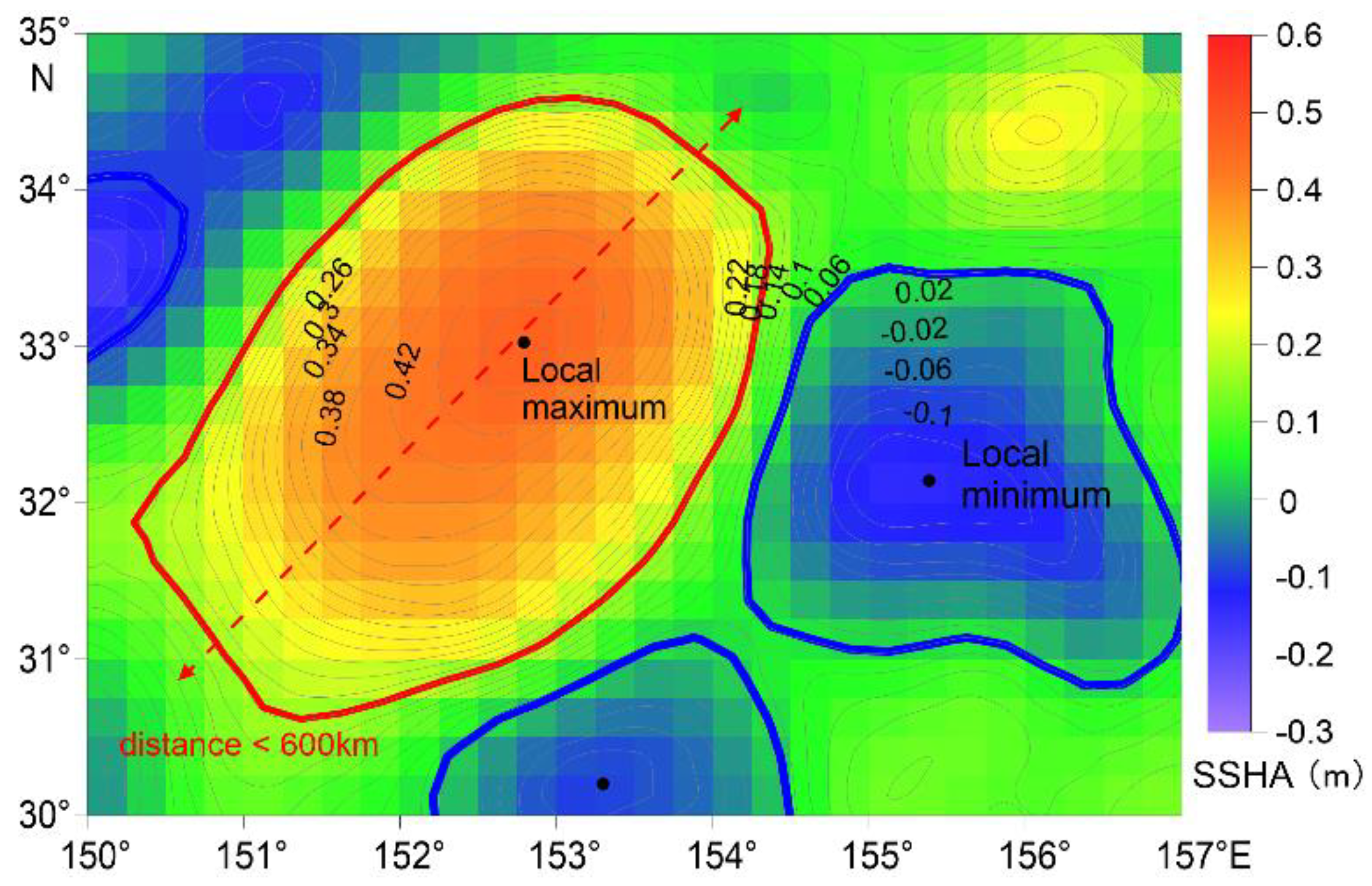
2.2.1. SSHA-Based Eddy Identification and Tracking

Mesoscale eddies can cause sea surface to rise or fall due to the geostrophic motion, which can be easily observed by satellite altimeter measurements. Eddies can generally be identified as enclosed regions in the SSHA field. The authors of [4] proposed using the outermost closed contour of SSHA to determine the eddy area. The geometric algorithm based on SSHA contours is widely used in mesoscale eddy identification [31,38]. Specifically, for each local extremum in the SSHA field, the algorithm searches for an area that meets some certain conditions and considers it to be an eddy [39] (Figure 1):
(1)
The SSHA values of all internal grids are greater (less) than that of the outmost contour for anticyclonic (cyclonic) eddies.
(2)
The number of internal grids is ≥8 and <1000.
(3)
There is only one local SSHA maximum (minimum) for anticyclonic (cyclonic) eddies. The local extremum point is seen as an eddy center.
(4)
The amplitude of the eddy is ≥3 cm for avoiding the interference of SSH noise from the system error in satellite altimeters [40,41]. The amplitude of an eddy is defined as the absolute value of the SSHA difference between the eddy center and its boundary.
(5)
The distance between any two internal grids is <600 km for avoiding enclose elongated region.
Based on the daily SSHA field, the mesoscale eddies in the Kuroshio Extension are identified, and the eddy amplitude and eddy radius scale are quantified over the study region. The trajectory of one eddy moving in the ocean can be tracked by comparing the eddy identification results in the continuous time series of the daily SSHA field. For one eddy at the time dayn, the tracking algorithm compares the eddy characteristics and searches for the most similar eddy at the next time dayn+1 within a circle of eddy radius as its successor [42,43]. In order to avoid missing identification and false tracking of eddies, the tracking algorithm will repeat the same operation for the next 10 days when no matching result is found at the next time dayn+1 [39]. Considering that the gridded SLA fields are merged using three altimeters (after the year 2000), the gap between satellite ground tracks is less than 50 km at 10° latitude. If an eddy moves westward with a speed of 5 cm·s−1 in the ocean, then, after 10 days, it will have ~40 km displacement, which is enough to capture the eddy signal at the neighboring ground track. The lifetime of an eddy represents the duration of an eddy from its generation to its termination.

2.2.2. SSTA-Based Eddy Identification and Matching

Figure 2 shows an SSHA map, an SSTA map, and eddy results identified from SSHA field. It can be seen that the SSHA map and SSTA map have a high similarity; high/low SSHA structures correspond to high(warm)/low(cold) SSTA ones. Therefore, similar to the SSHA-based eddy identification, an enclosed region of SSTA is used to identify mesoscale eddies from SSTA field [44]. Eddies with low SSTA are cold eddies (cyclones), and eddies with high SSTA are warm eddies (anticyclones) (Figure 3). The conditions of SSTA-based eddy identification are the same as those of SSHA-based eddy identification, except that the condition 4 became “The temperature amplitude of the eddy was at least 0.3 °C”. The experiment found that the vortex-like shape with an amplitude of less than 0.3 °C is irregular and unstable. In this method, the eddy result from SSTA field can be obtained. The SSTA-based eddy tracking is the same as that of SSHA.
Based on SSHA and SSTA fields, mesoscale eddies in the Kuroshio Extension were identified through the eddy identification procedure, respectively. In order to match the eddy results of the two data, we used an overlapping ratio α, which is the overlapping area of the two eddies divided by the area of the smaller one, to confirm the spatial relationship of SSHA- and SSTA-based eddies on the same day. If the overlapping ratio α of the two eddies is greater than 0.5 (e.g., Figure 3), the two eddies will be considered as matched eddies in the correlation analysis of SSHA and SSTA signals of eddies. Then, the mean SSHA and SSTA of matched eddies were calculated and a scatterplot of SSHA–SSTA within matched eddies was obtained. Based on the scatterplot, a linear regression analysis is used to estimate the linear relationship between SSHA and SSTA within matched eddies, SSTA = k·SSHA, where k is the regression coefficient measuring the SSHA–SSTA relationship. Sensitivity tests on the estimates of k with 95% confidence interval were performed.

2.2.3. Eddy Subsurface Signal from Argo Profiles

In order to study the subsurface structures of mesoscale eddies in the Kuroshio Extension, it is important to relate Argo profile data with the eddy signals at the sea surface from SSHA field or SSTA field. The subsurface temperature signal of eddies is obtained from the Argo float profiles inside SSHA- or SSTA-based eddy areas. For each eddy, we searched the Argo float profiles located in its boundary. We considered the identified eddies from the SSHA or SSTA field to match the Argo profiles on the same day and selected Argo profiles within eddies for subsurface temperature calculation. Thus, the Argo profiles are classified into three categories: Argo profiles inside cyclones, Argo profiles inside anticyclones, and other profiles outside eddies in this region. For the Argo profile matched by one eddy, we calculated the average θ′ at the subsurface depth as the subsurface signal of the eddy. Combining satellite altimetry data and Argo profiles, the study of the three-dimensional structure of eddies in the Kuroshio Extension showed that the subsurface temperature changes of eddies were mainly confined in the upper 800 dbar, especially in the depth of 100–500 dbar, at which eddies usually cause the greatest temperature change [23,31,33]. Therefore, we take the average value of the Argo θ′ at the depth of 100–500 dbar as the subsurface signal of eddies. Similar to the correlation analysis of SSHA and SSTA signals of eddies, by matching Argo profiles with SSHA- and SSTA-based eddies, the correlation and linear regression of SSHA–Argo θ′ and SSTA–Argo θ′ are analyzed, respectively.
The Kuroshio Extension (about 145°–170°E, 25°–45°N) is located in the northwest Pacific Ocean, which is dominated by the westerlies and easterly trade winds. In this study, the seasons are defined as winter (December–February), spring (March–May), summer (June–August), and autumn (September–November).

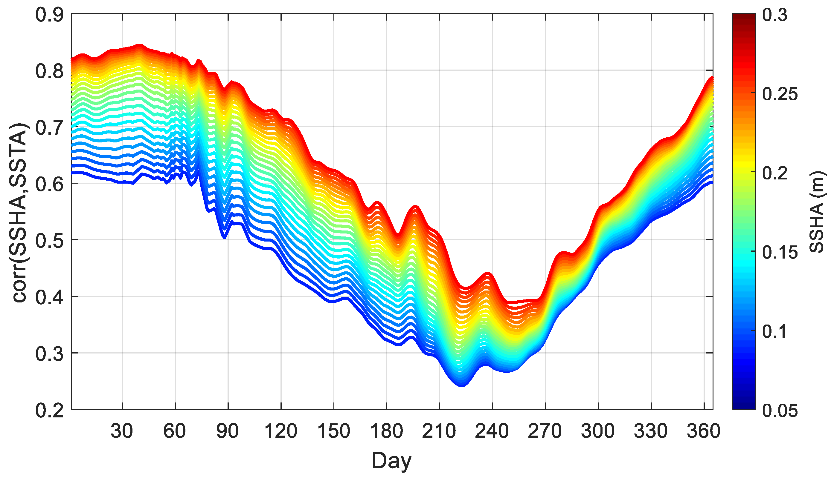
3. The Correlation between SSH and SST Data in Surface Signals of Mesoscale Eddies

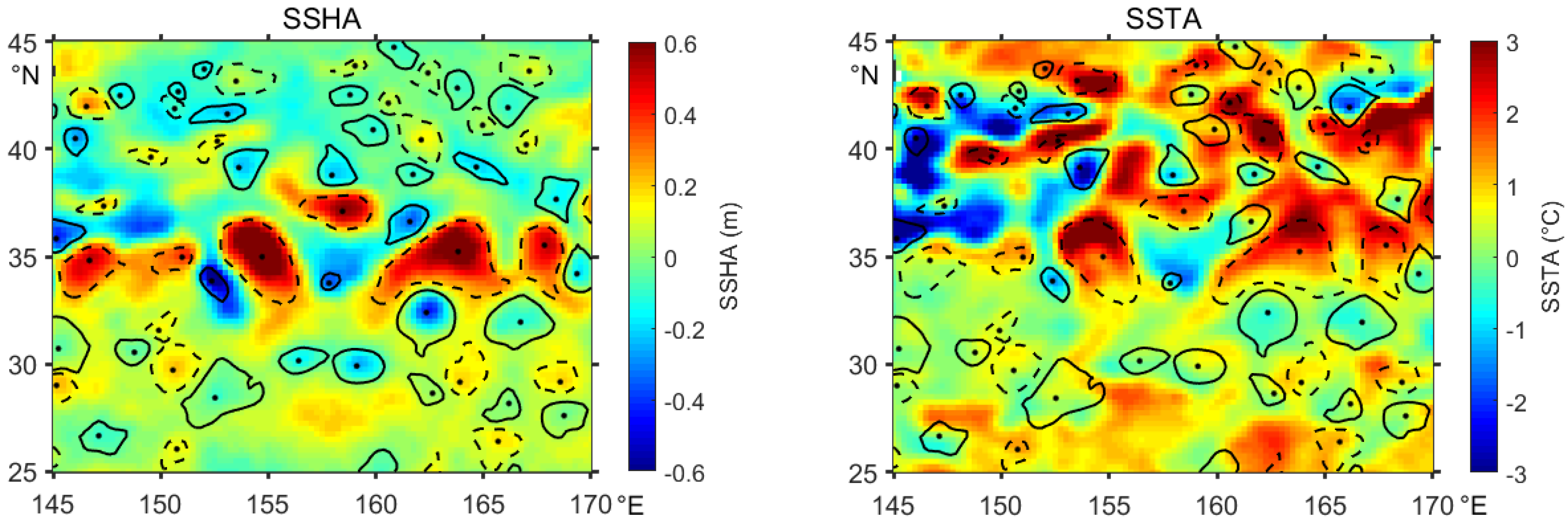
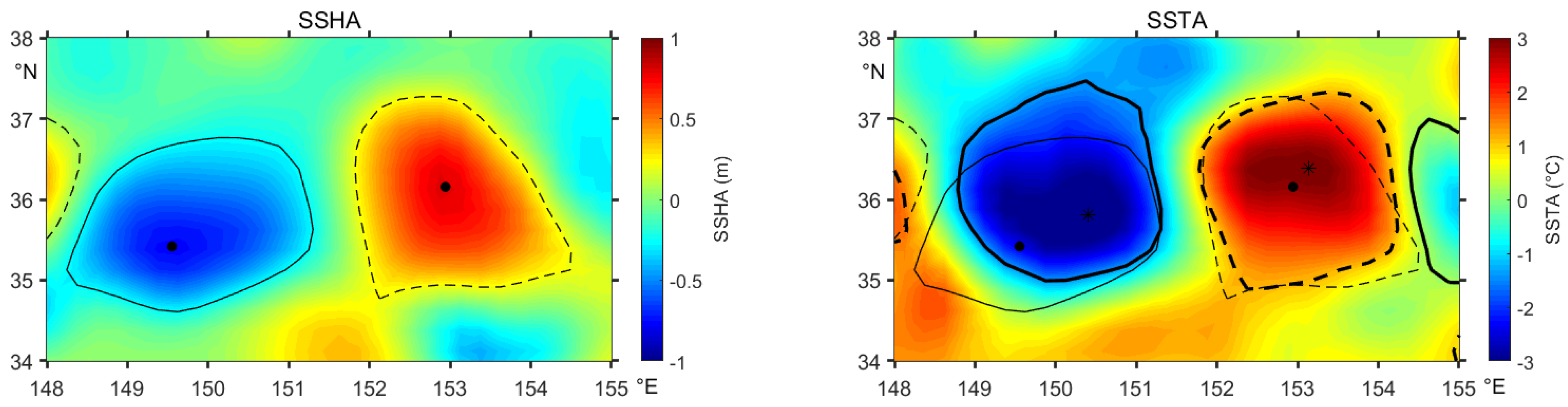
3.1. Eddy Signals in SSHA and SSTA Fields

Before analyzing the eddy signals in SSHA and SSTA fields, it is necessary to perform a correlation analysis on the two data in the Kuroshio Extension. For SSHA and SSTA fields, the correlation coefficient was calculated between SSHA field over a certain threshold (e.g., SSHA > 0.05m, 0.1m, 0.2m, etc.) and the corresponding SSTA field. Daily correlations between SSHA and SSTA fields for 1993–2021 in the whole Kuroshio Extension (145°–170°E, 25°–45°N) are shown in Figure 4. The result shows that SSHA and SSTA fields are generally more correlated in winter than in summer. Specifically, January (Figure 2 is a case) and August have the highest and lowest correlation values, respectively. This is because, in winter, the homogenization of the mixed layer is obvious and SST variance can then often match the subsurface temperature variance caused by oceanic mesoscale dynamic processes, while, in summer, the barrier layer on the surface prevents homogenization of the mixed layer. In addition, higher SSHA and SSTA have higher correlations, such as, when SSHA ≥ 20 cm, correlation values of SSHA and SSTA in January and February are usually greater than 0.8. It is shown that, at this time, the high SSHA variance generally corresponds to the high SSTA variance.
To analyze the seasonal correlation between the SSHA and SSTA signals of eddies, we matched eddy results identified from the two data and classified the same type of eddies (i.e., cyclonic-cold eddies and anticyclonic-warm eddies) according to seasons. Considering the geographical differences between the Kuroshio region and the Oyashio region, here, we divided the two regions with 38°N as the boundary to study the correlation of SSHA and SSTA signals within mesoscale eddies, respectively. The seasonal scatterplots of mean SSHA–SSTA within matched eddies for the Kuroshio region (the latitudes of 25°–38°N) and the Oyashio region (the latitudes of 38°–45°N) are shown in Figure 5. As a result, there are 33,837, 34,835, 19,259, and 19,009 matched eddies in the Kuroshio region and 28,788, 20,910, 17,785, and 23,947 matched eddies in the Oyashio region for SSHA- and SSTA-based results in the seasons of winter, spring, summer, and autumn, respectively. The number of matched eddies shows obvious seasonal difference. The Kuroshio region has more matched eddies in winter and spring and has fewer matches in summer and autumn; the Oyashio region has more matches in winter and autumn and has fewer matches in spring and summer.
Based on the scatterplots of SSHA–SSTA within matched eddies, the linear regression coefficient k(SSTA/SSHA) with the error denoting its 95% confidence interval, as well as the correlation coefficient r, are given in Figure 5. The results show that regression coefficients k(SSTA/SSHA) are significantly different in different regions. The value of k in the Oyashio region (8–10 °C·m−1) is significantly larger than that in the Kuroshio region (3–4 °C·m−1); that is to say, eddies with the same SSHA signal have larger SSTA in the Oyashio region than in the Kuroshio region. Specifically, for the Oyashio region, the k(SSTA/SSHA) can reach a maximum of about 10 °C·m−1 in spring and is about 8–9 °C·m−1 in other seasons. The correlation coefficient r can reach 0.77 in winter and the lowest is 0.68 in summer. The k(SSTA/SSHA) of the Kuroshio region is the highest in winter, exceeding 4 °C·m−1, and about 3 °C·m−1 in other seasons. The correlation coefficient r can reach 0.84 in winter and the lowest is 0.66 in summer. The SSHA–SSTA correlation differences within eddies in the Kuroshio region and the Oyashio region are related to the local hydrological properties and eddy properties. In the Kuroshio region, the ocean dynamic process is vigorous, accompanied by abundant mesoscale eddies, which can cause large changes in sea surface dynamic height (i.e., SSHA, x-axis in Figure 5). However, the SST gradient in the Kuroshio region is small, and the SSTA caused by eddies is not significant. In contrast, in the Oyashio region, although the dynamic process is weak and the SSHA of eddies is small (generally less than 0.4m), the SST gradient is large, with some seasonal temperature front. Therefore, once an eddy appears there, it can cause large SSTA. The result is basically consistent with [23]; they suggested that the large k(SSTA/SSHA) relationship in the Oyashio region compared to the Kuroshio region is mainly attributed to the smaller thermal expansion coefficient, the stronger salinity compensation effect, as well as the shallower vertical structure of eddies.
In addition to matched eddies with the same type, based on SSHA- and SSTA-based eddy results, eddies with the opposite type (i.e., cyclonic-warm eddies and anticyclonic-cold eddies) were also matched with a spatial overlap ratio exceeding 0.5. The matched result shows that these abnormal eddies have the highest number in summer, with a total of 3517, the least in winter, with a number of 1632, and 2408 and 2669 in spring and autumn, respectively. These abnormal eddies are surprisingly abundant in the study area. Both the number of matched eddies with the same type and the number of matched eddies with the opposite type in different seasons show that eddies have better consistency between SSHA and SSTA signals in winter, while the two signals are less consistent in summer. The authors of [29] suggested that the pronounced seasonal cycle in the SSHA–SSTA correlation was associated with the seasonal variation of the surface mixed layer depth. Generally, the surface mixed layer was shallow in summer and eddy–wind interaction can potentially modify SSTA signal easier via the action of Ekman pumping of the upper ocean density surfaces; conversely, the surface mixed layer was generally at its depth in winter, making it hard to modify SSTA signal.

3.2. Eddy Signals in SSHA/SSTA Field and Subsurface Argo Profiles

The surface expression of mesoscale eddies is visible in satellite-derived SSHA and SSTA fields, and they are three-dimensional structures that reach down into the thermocline. Therefore, combining in situ Argo float profiles data, which can provide vertical temperature information inside eddies, the correlation between surface signals (SSHA/SSTA) and subsurface signals (vertical temperature information) of mesoscale eddies is analyzed (Figure 6). For the Argo profile captured by one eddy, we take the average value of the temperature anomaly θ′ at the depth of 100–500 dbar as the subsurface signal of the eddy in the Kuroshio Extension.
Correlation analysis shows that the correlation coefficient between SSHA signals and subsurface signals θ′ (SSHA–Argo θ′) in SSHA-based eddies (upper panels in Figure 6) is basically around 0.9 in the Kuroshio region (the latitudes of 25°–38°N), showing a good consistency in each season. The correlation coefficient in the Oyashio region (the latitudes of 38°–45°N) is basically around 0.7, slightly higher in autumn. Due to eddy activities in the Oyashio region being less intense than those in the Kuroshio region, the SSHA induced by eddies is small and the corresponding subsurface θ′ is also concentrated in the low value range. The linear regression coefficients k(θ′/SSHA) in the Kuroshio region and the Oyashio are both about 7–7.5 °C·m−1, with less seasonal changes. In other words, a 10 cm change in SSHA field caused by one eddy corresponds to a change of 0.7 °C in the subsurface temperature inside the eddy. The change in subsurface temperature within eddies is significantly higher than the change in SSTA signals in the Kuroshio region but lower than the change in SSTA signals in the Oyashio region.
Compared with the SSHA-based eddies, SSTA signals and Argo subsurface signals θ′ (SSTA–Argo θ′) in SSTA-based eddies (bottom panels in Figure 6) have obviously regional and seasonal changes. The SSTA–Argo θ′ in both the Kuroshio and Oyashio region have the largest correlation in winter, both with the correlation coefficient of 0.76, and the lowest correlation in summer, with correlation coefficients of 0.45 and 0.42, respectively. The correlation is significantly lower than the result of SSHA–Argo θ′. This seasonal correlation is basically consistent with the seasonal variation in the correlation between SSHA and SSTA within eddies. Moreover, in summer, the SSTA–Argo θ′ correlation is very weak, which indicates surface eddy signals detected based on SSTA field are probably not stable eddy structures but more likely signal interference in SST fields due to the seasonal influence of the mixed-layer depth and atmospheric forcing. The SSTA signals in eddies are basically between −4 °C and 4 °C, while the subsurface signals θ′ are larger, which can reach ±8 °C in the Kuroshio region. This shows that the mesoscale eddy does not always have the most significant signal in the surface or may not appear in the surface. For example, in summer, it has a strong temperature anomaly signal in the subsurface but with a weak SSTA signal in the surface. The linear regression coefficient k(θ′/SSTA) in the Kuroshio region is about 1.3 in autumn and winter, about 1 in spring, and a minimum of 0.91 in summer. The linear regression coefficient k(θ′/SSTA) in the Oyashio region is less than 1 in all seasons; values are 0.74, 0.54, 0.45, and 0.62 in the seasons of winter, spring, summer, and autumn, respectively. The SSTA magnitude of eddies in the Kuroshio region is basically equal to the magnitude of subsurface temperature changes, while the SSTA of eddies in the Oyashio region is about twice the subsurface temperature changes.
In addition, by relating Argo profiles with the matched eddies (the result of Figure 5) from SSHA and SSTA data (i.e., the three SSHA, SSTA, and Argo signals in the same eddy), the correlation between surface SSHA/SSTA signals and Argo θ′ of the SSHA–SSTA matched eddies are analyzed (figure not shown). As a result, there are 1521, 1155, 758, and 926 matched eddies for SSHA, SSTA, and Argo profiles in the seasons of winter, spring, summer, and autumn, respectively. The seasonal scatterplots of SSHA–Argo θ′ and SSTA–Argo θ′ in these eddies are similar with the result of Figure 6. However, compared with SSHA- or SSTA-based eddies from a single remote sensing datum (Figure 6), the correlations of SSHA–Argo θ′ and SSTA–Argo θ′ of matched eddies from both SSHA and SSTA data are generally higher. For example, the SSHA–Argo θ′ correlation coefficient r of SSHA–SSTA matched eddies can reach the highest of 0.95 in summer and autumn, and SSTA–Argo θ′ correlation coefficient r can reach the highest of 0.84 in winter. The result indicates that eddy identification result from the two remote sensing data has better consistency between surface signals and subsurface signals. This implies that eddies detected by both SSHA and SSTA data are more likely consistent coherent structures, rather than unstable transient turbulence, which shows the potential of combining SSHA and SSTA data to detect mesoscale eddies.

4. Eddy Result Comparison from SSHA and SSTA Data

The trajectory of one eddy moving in the ocean can be tracked by comparing the eddy identification results in the continuous time series of the SSHA and SSTA fields. A statistical analysis of the eddy trajectories from the year 1993 to 2021 in the Kuroshio Extension is presented in this section. Eddy number, lifetime, propagation distances, geographical distribution, and eddy properties are compared from 29 years of SSHA and SSTA data.

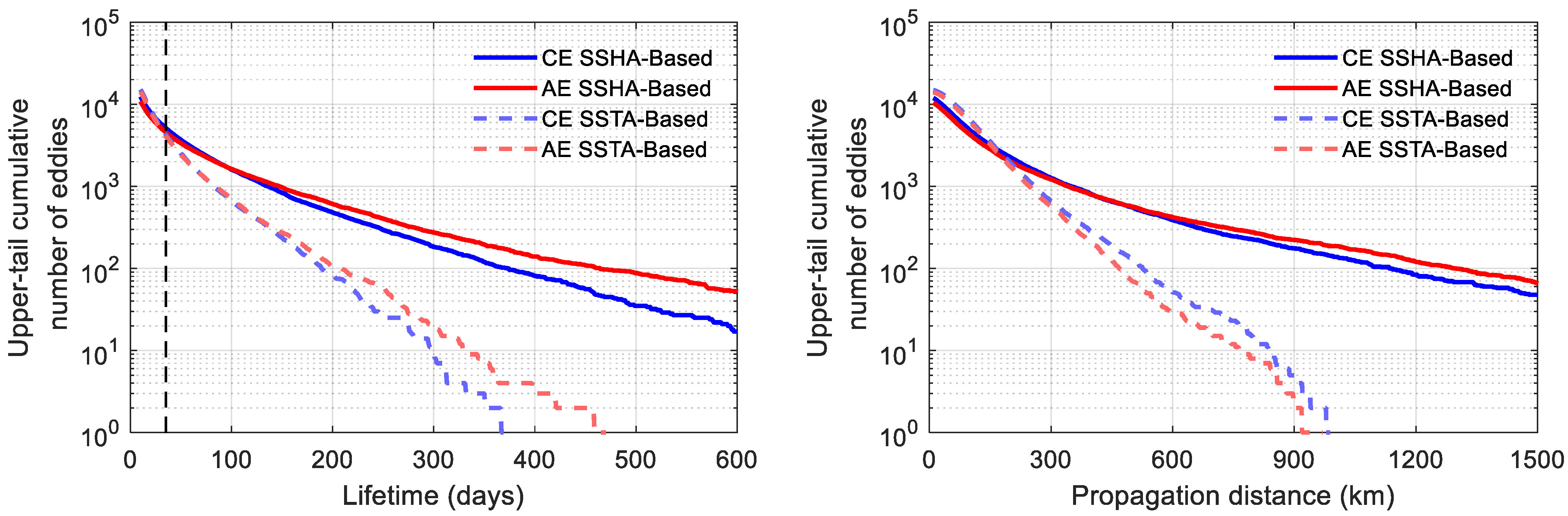
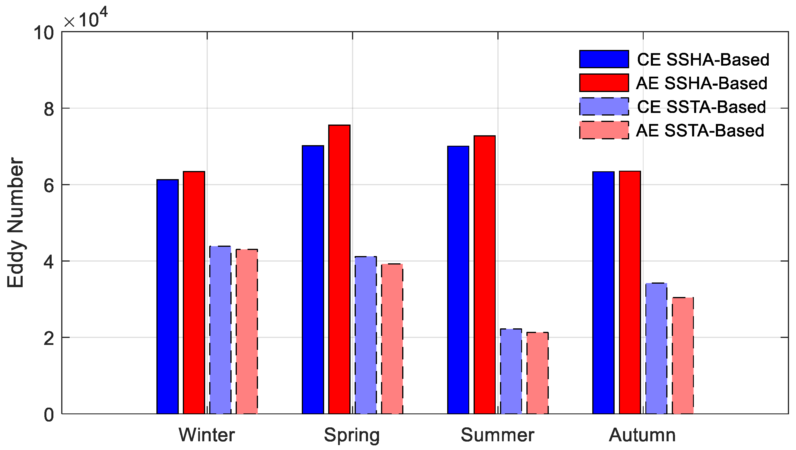
4.1. Eddy Number, Lifetime, and Propagation Distances

The upper-tail cumulative histograms of the eddy lifetimes and the propagation distances are shown separately for SSHA- and SSTA-based eddies in Figure 7. As a result, for both SSHA- and SSTA-based eddies, the number of eddy trajectories decrease rapidly with the increasements in the lifetime and the propagation distance, especially for SSTA-based eddies. For long lifetimes or propagation distances, the SSTA-based result is significantly lower than the SSHA-based result. For example, rare SSTA-based eddy trajectories have a lifetime over 360 days (about 1 year) and a propagation distance over 1000 km. In contrast, many SSHA-based eddy trajectories can exist over 360 days or longer and propagate over 1000 km or further.
To avoid the interference of the transient vortex-like structures and to obtain consistent coherent structure in this study [41], we focus attention on the eddies with lifetime ≥ 30 days and ignore eddies with shorter lifetime. As a result, 5037 anticyclonic trajectories and 5685 cyclonic trajectories detected from SSHA field, as well as 4763 anticyclones and 5062 cyclones detected from SSTA field, are analyzed in the following research. The average lifetime and propagation distance of SSHA-based eddy trajectories with lifetime ≥ 30 days are 98 days and 236 km, respectively, while the results of SSTA-based eddies are 63 days and 158 km. The lifetime and propagation distance of SSTA-based eddies are obviously shorter and smaller than those of SSHA-based eddies. The shorter lifetime and propagation distance of SSTA-based eddies may be related to the rapid changes in SSTA field and the interference of small-scale oceanic signal in the SST field. Unlike satellite altimeter products, the unconnected small-scale variations are difficult to remove from the SST data, especially diurnal variations that tend to appear as random noise [45]. Therefore, a stable and continuous SSTA variation in mesoscale eddies is hard to maintain in the SST field for a long time.
The numbers of cyclonic and anticyclonic eddies from SSHA- and SSTA-based eddy trajectories with lifetime ≥ 30 days in different seasons are shown in Figure 8. Here, the “eddy” is distinguished from eddy trajectory, which is the result of eddy identified from daily SSHA or SSTA field. In other words, eddies in the continuous time form the eddy trajectory. It can be seen that the numbers of SSHA-based eddies are higher than SSTA-based eddies in all seasons. This is mainly because the lifetime of SSTA-based eddy trajectories is relatively short, resulting in a small number of eddies. Comparing with SSHA-based eddies, the number of SSTA-based eddies varies greatly with the season, with more eddies in winter and fewer eddies in summer. The seasonal variation in the number of SSTA-based eddies is consistent with the correlation between SSHA and SSTA fields in Section 3.1. This indicates that, due to the homogenization of the mixed layer in winter, temperature changes caused by eddies can be more easily revealed in the surface SSTA field. In contrast, the stratification effect is obvious in summer, which prevents surface temperature changes caused by eddies, so the surface temperature is difficult to “capture” from eddy signals. As a result, there are fewer eddies identified from SSTA field than SSHA field in summer.

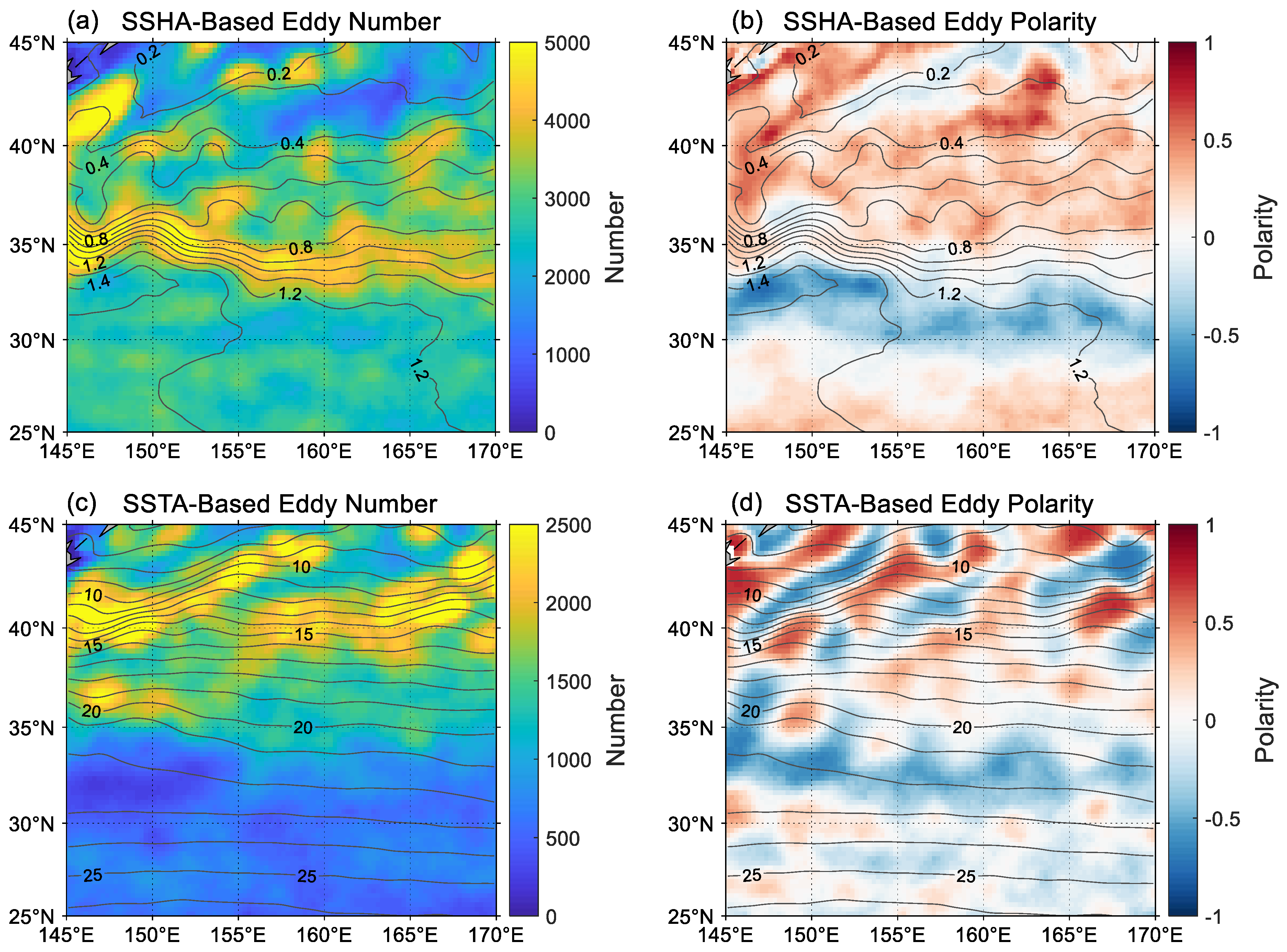
4.2. Eddy Geographical Distribution and Polarity

Mesoscale eddies are not evenly distributed in the ocean but are concentrated in some regions. To reveal the geographical distribution of eddies in the Kuroshio Extension, the number of eddies passing through each grid of 0.25° × 0.25° is counted. The maps of eddy number from eddy trajectories with lifetime ≥ 30 days are shown in Figure 9. For SSHA-based eddies (Figure 9a), we can see that mesoscale eddies exist primarily around the region of the Kuroshio mainstream (33°–36°N). The high eddy kinetic energy and root mean square of the SSHA in the region of the Kuroshio mainstream indicate frequent activities and strong intensity of eddies are distributed here [4,31]. By contrast, SSTA-based eddies (Figure 9c) are concentrated in the region north of the Kuroshio mainstream, especially near the Oyashio Extension (39°–42°N). The SST contours are denser there, indicating that the SST gradient is large and there is a certain temperature front (the Oyashio Front). Changes in SST field caused by mesoscale eddies are more obvious and more likely to be captured by satellites there. Compared with SSHA-based eddies, SSTA-based eddies are less abundant in the Kuroshio mainstream and the south side. This is related to the smaller SST gradient there. The SST changes caused by eddies are not obvious, leading to these eddies not being able to be identified from SSTA field.
Eddy polarity P indicates that a region prefers cyclonic eddies (P < 0) or anticyclonic eddies (P > 0) [42]. It is calculated as P = (NAENCE)/(NAE + NCE), where NAE and NCE are the numbers of anticyclonic and cyclonic eddies in one region, respectively. The same as the geographical distribution of eddy number, the eddy polarity P at each grid is calculated and the corresponding polarity maps are displayed in Figure 9b,d. For both SSHA- and SSTA-based eddies, the south side of the Kuroshio (about 27°–33°N) tends to the occurrence of cyclonic eddies (cold eddies), while the north side of the Kuroshio (about 36°–40°N) tends to the occurrence of anticyclonic eddies (warm eddies). The preference of eddies on the north and south sides of the Kuroshio is easy to understand because vortices pinched off from the mainstream have cyclonic vorticity on the south side and anticyclonic vorticity on the north side. The cyclonic eddies carry cold water, moving from the north to the warm south, forming cold eddies; conversely, the anticyclonic eddies carry warm water, moving from the south to cold north, forming warm eddies [21,24]. The geographical distribution of eddy polarity in the Kuroshio Extension is consistent with the other regions of strong, meandering eastward currents, such as the Gulf Stream and the Agulhas Return Current [4,12,46]. In addition, in the region of the Kuroshio mainstream with the most frequent eddy activities, there is no obvious tendency for eddy polarity (P value is close to 0); the numbers of anticyclones and cyclones are basically equal.
In the Oyashio area (the north of 40°N), there are some differences in the geographical distribution of eddy polarity between SSHA-and SSTA-based eddies. The mismatch of eddy polarity from SSHA and SSTA data leads to more abnormal eddies there (i.e., cyclonic-warm eddy and anticyclonic-cold eddy) [28]. One possible explanation for this regional difference is that the large SST gradient and shallower surface mixed layer in the Oyashio area result in the SST signal being more sensitive to surface eddy–wind interaction. The eddy–wind interaction can modify SSTA signal via the action of Ekman pumping of the upper ocean density surfaces [29]. The reason for the inconsistency of eddy polarity between SSHA- and SSTA-based eddies needs further research in the future study. For SSTA-based eddies, the eddy polarity and the SST contour show a certain correlation. The SST contour in the region dominated by anticyclonic (warm) eddies (P > 0) is convex, while the SST contour in the region dominated by cyclonic (cold) eddies (P < 0) is concave. This indicates that the region where eddies are concentrated will change the climatological SST distribution.

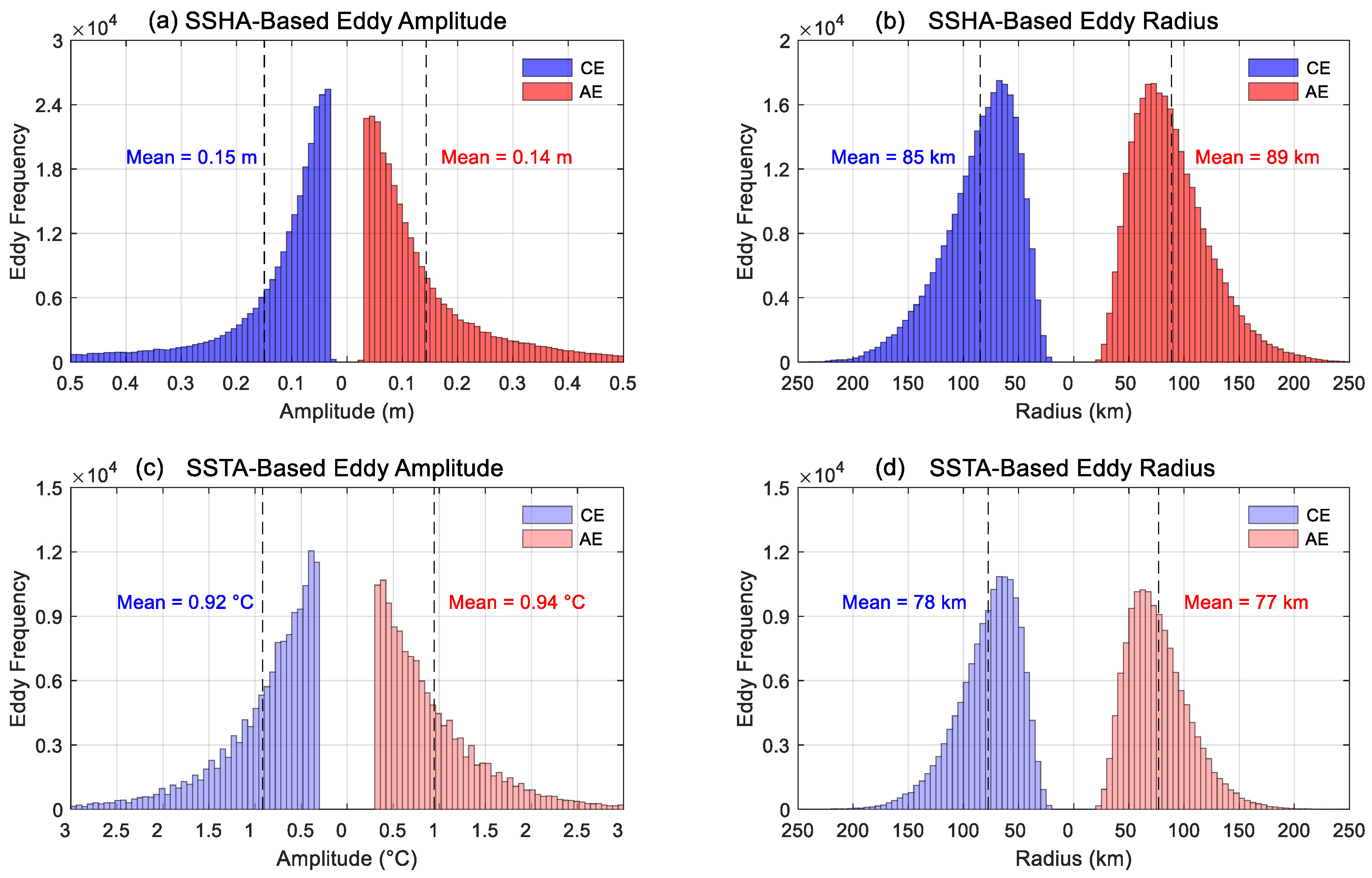
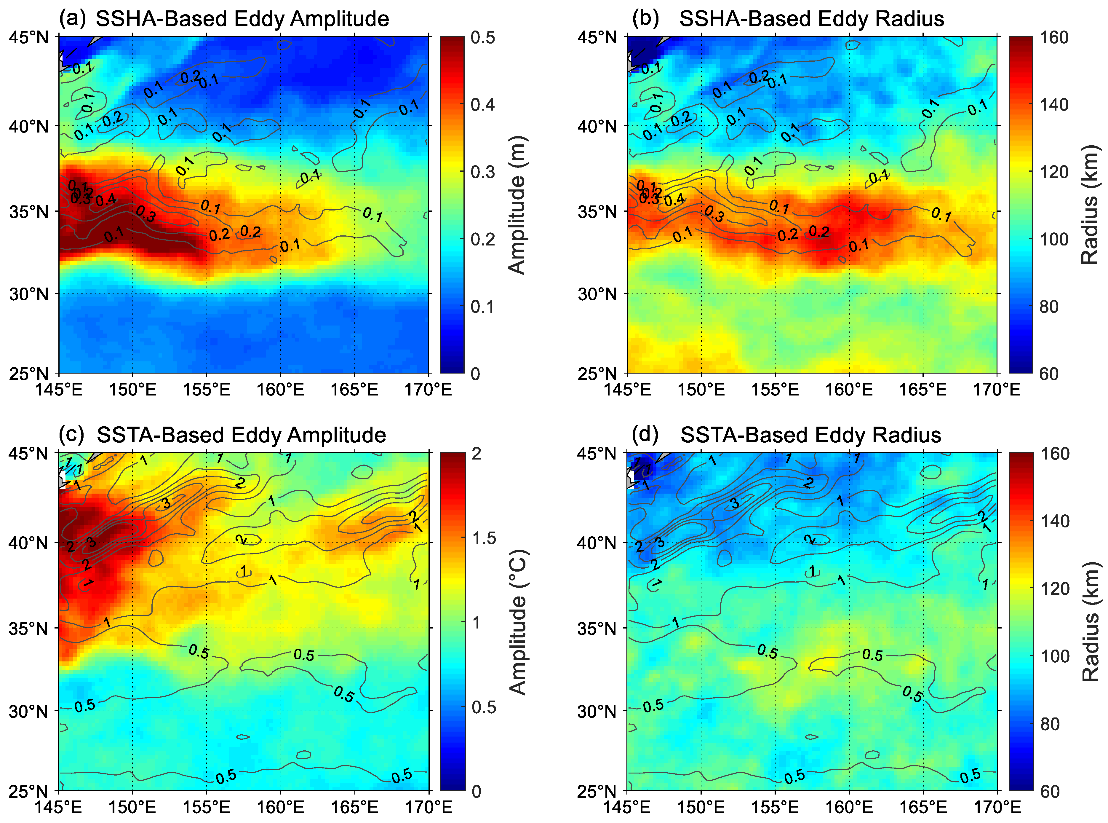
4.3. Eddy Properties

The eddy identification procedure provides property information of the eddy amplitude and radius scale, as defined in Section 2.2. The eddy amplitude and radius scale of SSHA- and SSTA-based eddy trajectories with lifetime ≥ 30 days over a 29-year period are analyzed in this section. Histograms of the eddy amplitudes and radius scales for SSHA- and SSTA-based eddies are shown in Figure 10, respectively. For both SSHA- and SSTA-based eddies, the eddy amplitudes are broadly distributed. However, eddies tend to be concentrated in the range of small amplitudes. Statistically, about half of the SSHA-based eddies have amplitude < 10 cm, and two thirds of the SSTA-based eddies have amplitude < 1 °C. Separately, the average amplitudes of SSHA-based cyclonic and anticyclonic eddies are 15 cm and 14 cm, and those of SSTA-based eddies are 0.92 °C and 0.94 °C. More than 90% of SSHA- and SSTA-based eddies have radius scales between 40 km and 150 km. SSTA-based eddies are more skewed toward small radius scales than SSHA-based eddies. On average, the average radii of SSHA-based cyclonic and anticyclonic eddies are 85 km and 89 km, and those of SSTA-based eddies are 78 km and 77 km, respectively.
The geographical distribution of eddy amplitudes is very similar in pattern and magnitude to the absolute dynamic topography (ADT) and SST gradient (Figure 11a,c). For SSHA-based eddies, the large-amplitude eddies occur in the region of the Kuroshio mainstream, especially in the west of 155°E, where the eddy amplitudes can exceed 50 cm. Over the rest of the regions, the eddy amplitudes are generally less than 20 cm. For SSTA-based eddies, the large-amplitude eddies are found in the Oyashio and its extension, where the eddy amplitudes can exceed 2 °C. In Section 3.1, SSHA and SSTA signals in eddies show a different regression relationship in the Kuroshio region and Oyashio region. The regional difference is also reflected in the geographic distribution of eddy amplitude from SSHA and SSTA data. In the region of Kuroshio mainstream, the amplitude of SSHA-based eddies is significantly high, but the amplitude of SSTA-based eddies is generally low. In contrast, the amplitude of SSHA-based eddies is low but with high amplitude of SSTA-based eddies in the Oyashio region. The regional difference in the eddy signal leads to the fact that the regression relationship of SSHA and SSTA signals is larger in the Oyashio region than in the Kuroshio region.
The difference is more obvious in the geographical distribution of the eddy radius scales (Figure 11b,d). Mesoscale eddies in the region of the Kuroshio mainstream are vigorous and have a large spatial scale. However, the eddy radius of SSTA-based eddies is not as large as that of SSHA-based eddies. SSHA-based eddies have radius scales around 150 km in the region of the Kuroshio mainstream; in contrast, SSTA-based eddies only have radius scales about 110 km there. The smaller spatial scale of SSTA-based eddies may be related to the rapid changes in SSTA field and the interference of small-scale oceanic signal in the SST field; the eddy signal cannot be fully reflected in the SST field. The authors of [29] analyzed the three-dimensional structure of eddies and found that the SSTA signal in eddies can be divided into a monopole pattern due to vertical eddy isothermal displacement and a dipole pattern due to lateral eddy advection of background temperature. The dipole SSTA pattern may be identified as smaller-scale eddy in the SSTA-based eddy identification procedure. In addition, the mismatch of eddy polarity between SSHA- and SSTA-based eddies can also lead to the difference in the spatial scale of eddies. In addition, for both SSHA- and SSTA eddies, the eddy radius scales are small in the north and south region of the Kuroshio mainstream, especially in the north region (the Oyashio Extension) where the scales are less than 100 km.

5. Conclusions

In this study, we used SSH and SST fields derived from satellite measurements and in situ data of Argo float profiles to study the correlation between SSHA and SSTA data in surface signals of mesoscale eddies in the Kuroshio Extension. Then, a comparative analysis of eddy results from SSHA and SSTA data is carried out, e.g., eddy numbers, eddy sizes, eddy amplitudes, and geographical distribution of eddies.
To analyze the seasonal correlation between the SSHA and SSTA signals of eddies, we matched eddy results identified from the two data and classified the same type of eddies according to seasons. The seasonal scatterplots of mean SSHA–SSTA within matched eddies indicates that regression coefficients k(SSTA/SSHA) are significantly different in different regions. The linear regression coefficient k in the Oyashio region (8–10 °C·m−1) is significantly larger than that in the Kuroshio region (3–4 °C·m−1); that is to say, eddies with the same SSHA signals have larger SSTA in the Oyashio region than in the Kuroshio region. SSHA–Argo θ′ in eddies show a high correlation with a regression coefficient k(θ′/SSHA) of about 7 °C·m−1 in all seasons. Meanwhile, for SSTA–Argo θ′, the correlations have obviously seasonal changes, with high value in winter and low value in summer. In addition, SSTA signals in eddies are basically between –4 °C and 4° C, while subsurface signals θ′ are larger, which can reach ±8 °C. This shows that the mesoscale eddy does not always have the most obvious signal in the surface or may not appear in the surface, such as, in summer, it has a strong temperature anomaly signal in the subsurface but a weak SSTA signal in the surface. In addition, compared with SSHA- or SSTA-based eddies from a single remote sensing datum, eddies detected by both SSHA and SSTA data have better consistency between surface signals and subsurface signals, which shows the potential of combining SSHA and SSTA data to detect mesoscale eddies.
A statistical analysis of the eddy trajectories with lifetime ≥ 30 days in the Kuroshio Extension is presented in this study. Eddy properties in the Kuroshio Extension are compared from 29 years of SSHA and SSTA data. The results show that the lifetime and propagation distance of SSTA-based eddies are shorter and smaller than that of SSHA-based eddies. The shorter lifetime and propagation distance of SSTA-based eddies may be related to the rapid changes in SSTA field and the interference of small-scale oceanic signal in the SST field. The seasonal variation in the number of SSTA-based eddies, with the highest in winter and the lowest in summer, is consistent with the correlation between SSHA and SSTA fields. This indicates that, due to the homogenization of the mixed layer in winter, temperature changes caused by mesoscale eddies can be more easily revealed in the surface SSTA field. In contrast, the eddy–wind interaction is obvious in summer, which weakens surface temperature changes caused by eddies, so the surface temperature is difficult to “capture” eddy signals. The geographical distribution of the eddies reveals that SSHA-based eddies exist primarily around the region of the Kuroshio mainstream (33°–36°N), while SSTA-based eddies are concentrated in the Oyashio Extension (39°–42°N). Both SSHA- and SSTA-based eddies show an inhomogeneity in the geographical distribution of eddy polarity. Mesoscale eddy is predominantly cyclonic on the southward side of Kuroshio and anticyclonic on the northward side.
The final census statistic of eddy properties shows that about half of the SSHA-based eddies have amplitude < 10 cm and two thirds of the SSTA-based eddies have amplitude < 1 °C. SSHA-based eddies with large amplitude occur in the region of the Kuroshio mainstream, especially in the west of 155°E, where the eddy amplitudes can exceed 50 cm. For SSTA-based eddies, the large-amplitude eddies are found in the Oyashio Extension, where the eddy amplitudes can exceed 2 °C. The geographical distribution of eddy amplitudes is very similar in pattern and magnitude to the ADT and SST gradient. More than 90% of SSHA- and SSTA-based eddies have radius scales between 40 km and 150 km. The radius scales of SSHA-based eddies are larger than those of SSTA-based eddies. The difference is more obvious in the geographical distribution of the eddy radius scales. SSHA-based eddies have radius scales around 150 km in the region of the Kuroshio mainstream; in contrast, SSTA-based eddies only have radius scales of about 110 km there.

Author Contributions

J.Y. and J.Z. designed the experiments and W.C. and Y.J. carried them out. W.C. performed the data analyses and drafted the paper. W.C. prepared the manuscript with contributions from all co-authors. All authors have read and agreed to the published version of the manuscript.

Funding

This work was supported by the National Natural Science Foundation of China (Grant No. 42106178), the Basic Scientific Fund for National Public Research Institutes of China (Grant No. 2020Q07), the Science Foundation of Donghai Laboratory (Grant No. DH-2022KF01014), and the Shandong Provincial Natural Science Foundation (Grant No. ZR2021QD006).

Data Availability Statement

The multi-altimeter merged SSH products (SEALEVEL_ GLO_PHY_L4_REP_OBSERVATION_008_47) used here were produced by Ssalto/Duacs and distributed by the European Copernicus Marine Environment Monitoring Service (CMEMS, marine.copernicus.eu (accessed on 12 August 2022)). The daily Optimum Interpolation SST data from AVHRR were provided by NOAA (data.nodc.noaa.gov (accessed on 15 August 2022)). The Argo profiles are provided by Coriolis Global Data Acquisition Center of France (www.coriolis.eu.org (accessed on 20 August 2022)).

Acknowledgments

We thank three anonymous reviewers for helpful comments on an earlier version of this manuscript. We acknowledge all the data providers for the data utilized in this study.

Conflicts of Interest

The authors declare no conflict of interest.

References

  1. Fu, L.-L.; Cazenave, A. Satellite Altimetry and Earth Sciences: A Handbook of Techniques and Applications (Google EBook). In Satellite Altimetry and Earth Sciences A Handbook of Techniques and Applications; Elsevier: Amsterdam, The Netherlands, 2000. [Google Scholar]
  2. Robinson, I.S. Discovering the Ocean from Space; Springer: Berlin/Heidelberg, Germany, 2010. [Google Scholar]
  3. Thonet, H.; Lemonnier, B.; Delmas, R. Automatic Segmentation of Oceanic Eddies on AVHRR Thermal Infrared Sea Surface Images. In Proceedings of the Oceans Conference Record (IEEE), San Diego, CA, USA, 9–12 October 1995; Volume 1. [Google Scholar]
  4. Chelton, D.B.; Schlax, M.G.; Samelson, R.M. Global Observations of Nonlinear Mesoscale Eddies. Prog. Oceanogr. 2011, 91, 167–216. [Google Scholar] [CrossRef]
  5. Xu, C.; Shang, X.D.; Huang, R.X. Estimate of Eddy Energy Generation/Dissipation Rate in the World Ocean from Altimetry Data. Ocean Dyn. 2011, 61, 525–541. [Google Scholar] [CrossRef]
  6. Chaigneau, A.; Eldin, G.; Dewitte, B. Eddy Activity in the Four Major Upwelling Systems from Satellite Altimetry (1992–2007). Prog. Oceanogr. 2009, 83, 117–123. [Google Scholar] [CrossRef]
  7. Dong, C.; McWilliams, J.C.; Liu, Y.; Chen, D. Global Heat and Salt Transports by Eddy Movement. Nat. Commun. 2014, 5, 3294. [Google Scholar] [CrossRef] [PubMed] [Green Version]
  8. Chelton, D.B.; Gaube, P.; Schlax, M.G.; Early, J.J.; Samelson, R.M. The Influence of Nonlinear Mesoscale Eddies on Near-Surface Oceanic Chlorophyll. Science 2011, 334, 328–332. [Google Scholar] [CrossRef]
  9. Xu, G.; Dong, C.; Liu, Y.; Gaube, P.; Yang, J. Chlorophyll Rings around Ocean Eddies in the North Pacific. Sci. Rep. 2019, 9, 1–8. [Google Scholar] [CrossRef] [Green Version]
  10. Zhang, Z.; Wang, W.; Qiu, B. Oceanic Mass Transport by Mesoscale Eddies. Science 2014, 345, 322–324. [Google Scholar] [CrossRef]
  11. Pascual, A.; Faugère, Y.; Larnicol, G.; le Traon, P.Y. Improved Description of the Ocean Mesoscale Variability by Combining Four Satellite Altimeters. Geophys. Res. Lett. 2006, 33, L02611. [Google Scholar] [CrossRef] [Green Version]
  12. Kang, D.; Curchitser, E.N. Gulf Stream Eddy Characteristics in a High-Resolution Ocean Model. J. Geophys. Res. Oceans 2013, 118, 4474–4487. [Google Scholar] [CrossRef]
  13. le Traon, P.Y.; Dibarboure, G. An Illustration of the Contribution of the TOPEX/Poseidon—Jason-1 Tandem Mission to Mesoscale Variability Studies. Mar. Geodesy 2004, 27, 3–13. [Google Scholar] [CrossRef]
  14. Stegner, A.; le Vu, B.; Dumas, F.; Ghannami, M.A.; Nicolle, A.; Durand, C.; Faugere, Y. Cyclone-Anticyclone Asymmetry of Eddy Detection on Gridded Altimetry Product in the Mediterranean Sea. J. Geophys. Res. Oceans 2021, 126, e2021JC017475. [Google Scholar] [CrossRef]
  15. Jones, M.S.; Allen, M.; Guymer, T.; Saunders, M. Correlations between Altimetric Sea Surface Height and Radiometric Sea Surface Temperature in the South Atlantic. J. Geophys. Res. Earth Surf. 1998, 103, 8073–8087. [Google Scholar] [CrossRef]
  16. D’alimonte, D. Detection of Mesoscale Eddy-Related Structures through Iso-SST Patterns. IEEE Geosci. Remote Sens. Lett. 2009, 6, 189–193. [Google Scholar] [CrossRef]
  17. Dong, C.; Nencioli, F.; Liu, Y.; McWilliams, J.C. An Automated Approach to Detect Oceanic Eddies from Satellite Remotely Sensed Sea Surface Temperature Data. IEEE Geosci. Remote Sens. Lett. 2011, 8, 1055–1059. [Google Scholar] [CrossRef]
  18. Trott, C.B.; Subrahmanyam, B.; Chaigneau, A.; Roman-Stork, H.L. Eddy-Induced Temperature and Salinity Variability in the Arabian Sea. Geophys. Res. Lett. 2019, 46, 2734–2742. [Google Scholar] [CrossRef]
  19. le Goff, C.; Fablet, R.; Tandeo, P.; Autret, E.; Chapron, B. Spatio-Temporal Decomposition of Satellite-Derived SST-SSH Fields: Links between Surface Data and Ocean Interior Dynamics in the Agulhas Region. IEEE J. Sel. Top. Appl. Earth Obs. Remote Sens. 2016, 9, 5106–5112. [Google Scholar] [CrossRef]
  20. Qiu, B.; Chen, S. Variability of the Kuroshio Extension Jet, Recirculation Gyre, and Mesoscale Eddies on Decadal Time Scales. J. Phys. Oceanogr. 2005, 35, 2090–2103. [Google Scholar] [CrossRef]
  21. Ji, J.; Dong, C.; Zhang, B.; Liu, Y.; Zou, B.; King, G.P.; Xu, G.; Chen, D. Oceanic Eddy Characteristics and Generation Mechanisms in the Kuroshio Extension Region. J. Geophys. Res. Oceans 2018, 123, 8548–8567. [Google Scholar] [CrossRef] [Green Version]
  22. Yang, H.; Qiu, B.; Chang, P.; Wu, L.; Wang, S.; Chen, Z.; Yang, Y. Decadal Variability of Eddy Characteristics and Energetics in the Kuroshio Extension: Unstable Versus Stable States. J. Geophys. Res. Oceans 2018, 123, 6653–6669. [Google Scholar] [CrossRef] [Green Version]
  23. Jing, Z.; Chang, P.; Shan, X.; Wang, S.; Wu, L.; Kurian, J. Mesoscale SST Dynamics in the Kuroshio-Oyashio Extension Region. J. Phys. Oceanogr. 2019, 49, 1339–1352. [Google Scholar] [CrossRef]
  24. Itoh, S.; Yasuda, I. Characteristics of Mesoscale Eddies in the Kuroshio-Oyashio Extension Region Detected from the Distribution of the Sea Surface Height Anomaly. J. Phys. Oceanogr. 2010, 40, 1018–1034. [Google Scholar] [CrossRef]
  25. Hausmann, U.; Czaja, A. The Observed Signature of Mesoscale Eddies in Sea Surface Temperature and the Associated Heat Transport. Deep Sea Res. Oceanogr. Res. Pap. 2012, 70, 60–72. [Google Scholar] [CrossRef]
  26. Leyba, I.M.; Saraceno, M.; Solman, S.A. Air-Sea Heat Fluxes Associated to Mesoscale Eddies in the Southwestern Atlantic Ocean and Their Dependence on Different Regional Conditions. Clim. Dyn. 2017, 49, 2491–2501. [Google Scholar] [CrossRef]
  27. Sun, W.; Dong, C.; Tan, W.; He, Y. Statistical Characteristics of Cyclonic Warm-Core Eddies and Anticyclonic Cold-Core Eddies in the North Pacific Based on Remote Sensing Data. Remote Sens. 2019, 11, 208. [Google Scholar] [CrossRef] [Green Version]
  28. Liu, Y.; Zheng, Q.; Li, X. Characteristics of Global Ocean Abnormal Mesoscale Eddies Derived From the Fusion of Sea Surface Height and Temperature Data by Deep Learning. Geophys. Res. Lett. 2021, 48, e2021GL094772. [Google Scholar] [CrossRef]
  29. Ni, Q.; Zhai, X.; Jiang, X.; Chen, D. Abundant Cold Anticyclonic Eddies and Warm Cyclonic Eddies in the Global Ocean. J. Phys. Oceanogr. 2021, 51, 2793–2806. [Google Scholar] [CrossRef]
  30. Chaigneau, A.; le Texier, M.; Eldin, G.; Grados, C.; Pizarro, O. Vertical Structure of Mesoscale Eddies in the Eastern South Pacific Ocean: A Composite Analysis from Altimetry and Argo Profiling Floats. J. Geophys. Res. Oceans 2011, 116, C11025. [Google Scholar] [CrossRef]
  31. Yang, G.; Wang, F.; Li, Y.; Lin, P. Mesoscale Eddies in the Northwestern Subtropical Pacific Ocean: Statistical Characteristics and Three-Dimensional Structures. J. Geophys. Res. Oceans 2013, 118, 1906–1925. [Google Scholar] [CrossRef]
  32. Amores, A.; Melnichenko, O.; Maximenko, N. Coherent Mesoscale Eddies in the North Atlantic Subtropical Gyre: 3-D Structure and Transport with Application to the Salinity Maximum. J. Geophys. Res. Oceans 2017, 122, 23–41. [Google Scholar] [CrossRef]
  33. Dong, D.; Brandt, P.; Chang, P.; Schütte, F.; Yang, X.; Yan, J.; Zeng, J. Mesoscale Eddies in the Northwestern Pacific Ocean: Three-Dimensional Eddy Structures and Heat/Salt Transports. J. Geophys. Res. Oceans 2017, 122, 9795–9813. [Google Scholar] [CrossRef]
  34. AVISO. SSALTO/DUACS User Handbook: MSLA and (M)ADT Near-Real Time and Delayed Time Products. CLS-DOS-NT-06-034, Issue 5.0, Cnes, France, 2016. Available online: https://www.aviso.altimetry.fr/fileadmin/documents/data/tools/hdbk_duacs.pdf (accessed on 10 January 2021).
  35. Picot, N.; Lachiver, J.M.; Lambin, J.; Poisson, J.C.; Legeais, J.F.; Vernier, A.; Thibaut, P.; Lin, M.; Jia, Y. Towards An Operational Use Of Hy-2a In Ssalto/Duacs: Evaluation Of The Altimeter Performances Using Nsoas S-Igdr Data. In Proceedings of the Ocean Surface Topography Science Team Conference (OSTST), Boulder, CO, USA, 8–11 October 2013. [Google Scholar]
  36. Reynolds, R.W.; Smith, T.M.; Liu, C.; Chelton, D.B.; Casey, K.S.; Schlax, M.G. Daily High-Resolution-Blended Analyses for Sea Surface Temperature. J. Clim. 2007, 20, 5473–5496. [Google Scholar] [CrossRef]
  37. Banzon, V.F.; Reynolds, R.W.; Stokes, D.; Xue, Y. A 1/4°-Spatial-Resolution Daily Sea Surface Temperature Climatology Based on a Blended Satellite and in Situ Analysis. J. Clim. 2014, 27, 8221–8228. [Google Scholar] [CrossRef]
  38. Yi, J.; Du, Y.; Zhou, C.; Liang, F.; Yuan, M. Automatic Identification of Oceanic Multieddy Structures From Satellite Altimeter Datasets. IEEE J. Sel. Top. Appl. Earth Obs. Remote Sens. 2015, 8, 1555–1563. [Google Scholar] [CrossRef]
  39. Cui, W.; Yang, J.; Ma, Y. A Statistical Analysis of Mesoscale Eddies in the Bay of Bengal from 22–Year Altimetry Data. Acta Oceanol. Sin. 2016, 35, 16–27. [Google Scholar] [CrossRef]
  40. Dufau, C.; Orsztynowicz, M.; Dibarboure, G.; Morrow, R.; le Traon, P.Y. Mesoscale Resolution Capability of Altimetry: Present and Future. J. Geophys. Res. Oceans 2016, 121, 4910–4927. [Google Scholar] [CrossRef] [Green Version]
  41. Li, G.; Wang, Z.; Wang, B. Multidecade Trends of Sea Surface Temperature, Chlorophyll-a Concentration, and Ocean Eddies in the Gulf of Mexico. Remote Sens. 2022, 14, 3754. [Google Scholar] [CrossRef]
  42. Chaigneau, A.; Gizolme, A.; Grados, C. Mesoscale Eddies off Peru in Altimeter Records: Identification Algorithms and Eddy Spatio-Temporal Patterns. Prog. Oceanogr. 2008, 79, 106–119. [Google Scholar] [CrossRef]
  43. Chen, G.; Wang, D.; Hou, Y. The Features and Interannual Variability Mechanism of Mesoscale Eddies in the Bay of Bengal. Cont. Shelf Res. 2012, 47, 178–185. [Google Scholar] [CrossRef]
  44. Zhang, C.H.; Li, H.L.; Liu, S.T.; Shao, L.J.; Zhao, Z.; Liu, H.W. Automatic Detection of Oceanic Eddies in Reanalyzed SST Images and Its Application in the East China Sea. Sci. China Earth Sci. 2015, 58, 2249–2259. [Google Scholar] [CrossRef]
  45. Talley, L.D.; Pickard, G.L.; Emery, W.J.; Swift, J.H. Descriptive Physical Oceanography: An Introduction, 6th ed.; Academic Press: Cambridge, MA, USA, 2011. [Google Scholar]
  46. Zheng, S.; Du, Y.; Li, J.; Cheng, X. Eddy Characteristics in the South Indian Ocean as Inferred from Surface Drifters. Ocean Sci. 2015, 11, 361–371. [Google Scholar] [CrossRef]
Figure 1. Eddy identification based on gridded SSHA field. Squares with color represent 0.25° grid points of SSHA field, the thin grey lines represent SSHA contours, the thick red and blue lines represent eddy boundaries, and the black points represent eddy centers (local extrema).
Remotesensing 14 05776 g001
Figure 2. Maps of SSHA (left) and SSTA (right) on 4 January 2010 in the Kuroshio Extension; the solid and dashed lines represent cyclonic and anticyclonic eddies identified from SSHA field.
Remotesensing 14 05776 g002
Figure 3. SSHA-based eddy result (left, the thin lines) and SSTA-based eddy result (right, the thick lines) in the Kuroshio Extension; the solid and dashed lines represent cyclonic and anticyclonic eddies. In the right panel, the SSHA-based eddies are drawn with thin lines as a comparison with SSTA-based eddies.
Remotesensing 14 05776 g003
Figure 4. Daily correlations between SSHA and SSTA fields for 1993–2021 in the Kuroshio Extension (145°–170°E, 25°–45°N); the different colored lines indicate the correlation between SSHA field over a certain threshold (from 0.05 m to 0.3 m, with the interval of 0.01 m) and SSTA field.
Remotesensing 14 05776 g004
Figure 5. The seasonal scatterplots of mean SSHA and SSTA within matched eddies for the Kuroshio region (blue, the latitudes of 25°–38°N) and the Oyashio region (orange, the latitudes of 38°–45°N); the dotted lines are the linear regression of the scatterplots. The regression coefficient k (SSTA/SSHA) with the error denoting its 95% confidence interval, the correlation coefficient r, and numbers N of matched results are labeled in the figure.
Remotesensing 14 05776 g005
Figure 6. (Upper) The seasonal scatterplots of SSHA signals and Argo subsurface temperature anomalies θ′ in SSHA-based eddies. (Bottom) The seasonal scatterplots of SSTA signals and Argo subsurface temperature anomalies θ′ in SSTA-based eddies. The blue scatterplots are the result for the Kuroshio region (the latitudes of 25°–38°N) and the orange scatterplots are the result for the Oyashio region (the latitudes of 38°–45°N). The θ′ is computed as the average temperature anomaly of Argo profile within the eddy at depths of 100–500 dbar. The dashed lines are the linear regression of the scatterplots. The regression coefficient k (θ′/SSHA or θ′/SSTA) with the error denoting its 95% confidence interval, the correlation coefficient r, and numbers N of matched results are labeled in the figure.
Remotesensing 14 05776 g006
Figure 7. The upper-tail cumulative histograms of the lifetime (left) and the propagation distance (right) of cyclonic (CE) and anticyclonic (AE) eddy trajectories, respectively. The black dashed line represents the cutoff lifetime of 30 days; eddy trajectories with lifetime < 30 days are ignored in the following research.
Remotesensing 14 05776 g007
Figure 8. Seasonal statistical graph of the number of cyclonic (CE) and anticyclonic (AE) eddies from SSHA- and SSTA-based eddy trajectories with lifetime ≥ 30 days. Here, the “eddy” is distinguished from eddy trajectory, which is the result of eddy identified from the daily SSHA or SSTA field.
Remotesensing 14 05776 g008
Figure 9. The maps of eddy number and polarity distribution from SSHA-based (a,b) and SSTA-based (c,d) eddy trajectories with lifetime ≥ 30 days. Contours in panel a and b are the climatological mean absolute dynamic topography ADT (unit: m); contours in panel c and b are the climatological mean SST (unit: °C).
Remotesensing 14 05776 g009
Figure 10. Histograms of the amplitudes and radius scales from SSHA-based (a,b) and SSTA-based (c,d) eddy trajectories with lifetime ≥ 30 days for cyclonic (CE) and anticyclonic (AE) eddies. The dotted line represents the average value of eddy properties.
Remotesensing 14 05776 g010
Figure 11. The maps of the mean amplitude and radius scales from SSHA-based (a,b) and SSTA-based (c,d) eddy trajectories with lifetime ≥ 30 days. Contours in panel a and b are the gradient of climatological mean absolute dynamic topography ADT (unit: m/100 km); contours in panel c and b are the gradient of climatological mean SST (unit: °C/100 km).
Remotesensing 14 05776 g011
Publisher’s Note: MDPI stays neutral with regard to jurisdictional claims in published maps and institutional affiliations.

