Magnetization Vector Inversion Based on Amplitude and Gradient Constraints

Abstract

Magnetization vector inversion has been developed since it can increase inversion accuracy due to the unknown magnetization direction caused by remanence. However, the three components of total magnetizations vector are simultaneously inverted and then synthesized into the magnetization magnitude and direction, which increases the inherent non-uniqueness of the inversion. The positions of the three components of the magnetization vector are originally consistent. If there is a lack of constraints between them during the inversion process, they may be misaligned, resulting in a large deviation between the synthesized vector model and the ground truth. To address this issue and at the same time increase the accuracy of the edges of the inversion models, this paper proposes a magnetization vector inversion scheme with model and its gradients’ constraints by sparse Lp norm functions based on the amplitude of the three components of the magnetization vector instead of a single component to improve the accuracy of the inversion result. To evaluate the inversion accuracy performance, an improved evaluation index is also proposed in this paper, which can better evaluate the accuracy of the shape, position and magnetization amplitude of the inversion model. The proposed inversion method can recover the models with higher accuracy compared with traditional methods, indicated by the inverted model and the evaluation indexes. Simulation results based on the open-source SimPEG software and inversion on actual measured Galinge iron ore deposit (China) data verified the effectiveness and advantages of the proposed method.

1. Introduction

Magnetic vector inversion (MVI) can be applied to obtain the subsurface three-dimensional distribution including shape, position and magnetization magnitude and direction of magnetic targets with remanence, such as geological and mineral exploration [1,2,3] in geophysics. This also has important practical value in the study of magnetic distribution in spacecraft [4], accurate identification of important military targets [5], detection of underground ferromagnetic pipeline [6,7], detection of unexploded ordnance [8], and nondestructive testing [9]. Especially for the discrimination of dangerous objects, such as unexploded bombs, the shape of the high-precision 3D reconstruction can assist in accurate identification and reduce the risk of damage [10]. The accuracy of the inversion model is crucial for discriminating the shape of the inversion model.

Magnetic anomaly forward modeling, or magnetic response, is the basis for inversion. Many scholars have studied the forward modeling of gravity and magnetic anomalies of different models and given calculation formulas. Sharma [11] developed a rapid computation of magnetic anomalies due to a body of any shape with the aid of formulae derived for the field caused by a finite rectangular prism. Plouff [12] presented a forward calculation method for the gravitational and magnetic anomalies of a prism with polygonal cross-section and applied it to terrain correction. Guo et al. [13] deduced the theoretical expression of the total magnetic anomaly of the cuboid and its gradient field without analytical singularity in the upper half space. Ren et al. [14] computed accurate magnetic anomalies caused by realistic magnetic 3D structures.

The traditional scalar susceptibility inversion method assumes there is no remanent magnetization in the magnetic target and only considers the induced magnetization which is generally known. However, the total magnetization is the vector addition of the induced and remanent magnetizations. Remanent magnetization may cause the overall magnetization direction to be non-parallel to the geomagnetic field, leading to misleading interpretations [15]. There are many studies on how to deal with remanence [16,17,18,19,20,21,22], but magnetization vector inversion has more advantages for dealing with complex cases such as remanent magnetization in the object, which is more in line with the requirements of actual measurement.

Magnetization vector inversion divides the underground magnetization into three components for inversion to solve the problem of unknown magnetization direction caused by remanent magnetization. This method can invert magnetization amplitude and direction at the same time, but the unknown parameters to solve are three times that of the traditional scalar susceptibility inversion method [23], which in turn increases the nonuniqueness inherent in the inversion. This requires adding more constraints to the objective function.

Many studies on magnetization vector inversion have already been conducted. Parker et al. attempted to construct a three-component magnetization model using the semi-norm minimization procedure [24]. Wang et al. [25] developed a magnetization vector tomography imaging, but the method works for homogeneous objects separated by the overall magnetization direction. Lelievre and Oldenburg [26] presented a comprehensive study of magnetization vector inversion in Cartesian and spherical coordinates systems, respectively. In the Cartesian coordinate equation, the overall magnetization direction is divided into a component parallel and two components perpendicular to the geomagnetic field, constraining the three components of magnetization respectively. In the spherical coordinate equation, the three components of magnetization need to be converted into the magnitude and direction (i.e., declination and inclination) of magnetization for constraining inversion. Liu et al. [27] proposed a step-by-step magnetization vector inversion method. Firstly, the magnitude of the total magnetization was calculated from the magnetic amplitude data, and then the magnetization inclination and declination were calculated by means of correlation coefficient method or conjugate gradient inversion. In order to reduce the non-uniqueness of MVI, studies try to add more constraints to the objective function of optimization. Zhu et al. [28] added Gramian function to the objective function to constrain the three components. Results show that it can play a certain role, but the inversion results still need to be improved. Li and Sun [29] introduced a fuzzy c-means clustering algorithm in the objective function to constrain the magnetization direction. When the number of clusters is known, it can play a good role in constraining, otherwise, the inversion results will be affected. Fourier et al. [30,31] developed the magnetization vector inversion in the Cartesian and the spherical coordinate system, adding the oriented sparse Lp norm constraint to the objective function to obtain a model with a clearer boundary, especially for restoration of blocky models. The inversion results in the spherical coordinate system are better than those in the Cartesian coordinate system. But the former involves nonlinear transformation, which increases the complexity of the calculation and requires the well-developed initial model for inversion. Ghalehnoee et al. [32] further studied the algorithm in the Cartesian coordinate system and changed the sparse constraint function from the amplitude of a single component to the modulus of three components, increasing their mutual restraint. However, the results show that the corner information of the inverted block model is lost.

Currently, the accuracy of the 3D MVI in Cartesian coordinate system is not high enough. The reason is that the inversion problem itself has multiple solutions. When inverting three-component magnetization vector models at the same time, inconsistencies between the positions of them are prone to occur. Especially for the accuracy of the edge in MVI, the current method is still powerless. In addition, the evaluation of inversion results is usually judged by human subjectivity or by mean square error (MSE) [33] or root mean square error (RMSE) [34], which cannot reflect the inversion effect of edges. There is a lack of evaluation metrics that can evaluate the edge of the inversion model.

The purpose of this study is to improve the accuracy of the inversion. Under the regularized inversion framework, in the Cartesian coordinate system, we propose a magnetization vector inversion method with model and its gradient constraints by the sparse Lp norm based on the magnitude of the three-component magnetization models. The sparse Lp norm is useful for producing sparse solutions, easily getting models with sharp boundaries [30,35]. Constraining the three-component magnetization models with their amplitude will increase the constraints between them, and it is easy to obtain a vector model with higher accuracy. Sensitivity weighting [31] is used to counteract the decay of the magnetic signal with distance, and upper and lower bound constraints are used to further reduce the non-uniqueness of the inversion.

For the evaluation of inversion results, inspired by model shape similarity evaluation in computer vision, the intersection over union (IOU) index combining with the existing magnitude similarity measure RMSE, we propose a new evaluation index that can comprehensively evaluate the similarity of the shape, position and magnetization magnitude of the inversion model with the ground truth.

The proposed MVI method and the inversion evaluation index are validated by two synthetic examples. The results show that the inversion effects of the method proposed in this paper are superior to that of the traditional magnetization vector inversion method and the method in the previous study [32]. The inversion accuracy has been significantly improved, which can be indicated by the inverted model and evaluation indexes. In addition, the actual measured magnetic data of the Galinge iron ore deposit (China) are inverted using the proposed method in this paper. The inversion results are consistent with the real geological information. Since this method can obtain a high-precision model, it can be applied to large-scale mineral exploration and it has great potential for fields with high precision requirements, such as unexploded ordnance detection.

2. Methods

2.1. Amplitude and Gradient Constraints Based Magnetization Vector Inversion

In the inversion process, the model region is generally divided into orthogonal 3D grid magnetization cells with constant magnetic susceptibility. When total magnetization in jth cell can be expressed as

$${\overrightarrow{M}}_j={\kappa }_j{\overrightarrow{H}}_0+{\overrightarrow{M}}_{jrem}$$

(1)

where ${\kappa }_j$ and ${\overrightarrow{M}}_{jrem}$ are the magnetic susceptibility and remanent magnetization of jth cell, respectively, and $H_0$ is the earth’s magnetic field.

The magnetic field B at point ${\mathit{r}}_{\mathit{j}}$ resulting from a volume V containing magnetization in continuous form can be formulated by [15]

$$\mathit{B}\left({\mathit{r}}_{\mathit{j}}\right)=\nabla \int \mathit{M}\left(\mathit{r}\right)·\nabla \frac{1}{\left|\mathit{r}-{\mathit{r}}_{\mathit{j}}\right|}d{r}^3$$

(2)

where $\nabla$ is a differential operator.

The N data $d^{pre}={\left[d_1,\dots ,d_N\right]}^T$ predicted by discrete model can be calculated as

$$d^{pre}=Fm$$

(3)

where m = ${\left[{\kappa }_1, \dots ,{\kappa }_M\right]}^T$ is the model vector containing the magnetic susceptibility in each cell. F is an N-by-M forward operator which maps the contribution of M number of prisms, each contributing the response measured over N observed locations. The response of each small prism can refer to the paper [31].

The noise contained in the data is assumed to be independent and zero-mean Gaussian.

Different from the scalar susceptibility-based inversion, magnetization vector inversion divides the vector magnetization into three components for simultaneous inversion. The forward formula [31] in discrete system is as follows:

$$d^{pre}=Fm=\left[F_u{F}_v{F}_w\right]\left[\begin{array}{c}{\mathit{\kappa }}_u\\ {\mathit{\kappa }}_v\\ {\mathit{\kappa }}_w\end{array}\right]$$

(4)

$$d^{pre}\in {ℝ}^N {\mathit{F}}_u,{\mathit{F}}_v,{\mathit{F}}_w\in {ℝ}^{N\times M} m={\left[{\mathit{\kappa }}_u{\mathit{\kappa }}_v{\mathit{\kappa }}_w\right]}^T\in {ℝ}^{3M}$$

(5)

where $d^{pre}$ is predicted data. $F_u$, $F_v$ and $F_w$ are forward operators in three Cartesian directions respectively. Model m describes magnetization along the three Cartesian directions, which is three times the number of unknown parameters compared to the scalar susceptibility-based assumption. Specifically, $d^{pre}={\left[B_x, B_y, B_z\right]}^T$ is the three-component magnetic field data. F is a dense 3 by 3 symmetric matrix, described as follows:

$$F=\frac{{\mu }_0}{4\pi }\left[\begin{array}{ccc}{F}_{xx}& F_{xy}& F_{xz}\\ F_{xy}& F_{yy}& F_{yz}\\ F_{xz}& F_{yz}& F_{zz}\end{array}\right]$$

(6)

where ${\mu }_0$ is the magnetic permeability of free space. For the specific calculation formula of the F tensor, please refer to the article [31].

The inversion problem is formulated as an optimization problem where the Tikhonov objective function can be formulated as [36]

$$\varphi \left(m\right)={\varphi }_d+\beta {\varphi }_m \mathrm{subject} \mathrm{to} {\varphi }_d<{\varphi }_d{}^{*}$$

(7)

where ${\varnothing }_d$ is data misfit term, measuring the L2 norm of the data calculated by the subsurface model through forward formula and the observed data. ${\varnothing }_d{}^{*}$ is the target misfit and β is the regularization parameter. ${\varnothing }_m$ is the regularization term where prior information can be integrated. Further ${\varnothing }_d$ can be described as [31]

$${\varphi }_d=\sum _{i=1}^N\left(\frac{d_i^{pre}-d_i^{obs}}{{\sigma }_i}\right)=\Vert W_d{\left(Fm-d^{obs}\right)\Vert }_2^2,$$

(8)

where $d^{obs}$ is observed data. $W_d$ is the data weighting matrix generally determined by the inverse of the variance σ of the data, describing the noise level of the data. A more detailed ${\varnothing }_m$ formula can be described as [31]

$$\begin{array}{c}{\varphi }_m={\alpha }_s{\varphi }_s+{\alpha }_x{\varphi }_x+{\alpha }_y{\varphi }_y+{\alpha }_z{\varphi }_z=\\ {\displaystyle {\displaystyle \sum }_{c=u,v,w}}{\displaystyle {\displaystyle \sum }_{r=s,x,y,z}}{\alpha }_{c_r}\Vert W_{c_r}{V}_{c_r}{D}_{c_r}{\left(m-m_{ref}\right)\Vert }_2^2,\end{array}$$

(9)

where ${\varnothing }_s$, ${\varnothing }_x$, ${\varnothing }_y$, ${\varnothing }_z$ are the constraint functions of the models and their gradients in the three Cartesian directions and ${\alpha }_s$, ${\alpha }_x$, ${\alpha }_y$, ${\alpha }_z$ are the corresponding coefficients, respectively. The magnetization vector inversion applies the same constrained functions as above for the three-component models. Functions V and D are volumes of integration and discrete difference operators. The W is a combination of two weighting functions including sensitivity weighting function and the sparse constraint weighting function. The formula is as follows

$$W=W_P{W}_L$$

(10)

where $W_P$ acts like a depth weighting function [36] for counteracting the decay of the magnetic data with depth. Refer to the paper [31] for details.

$$W_P=\mathrm{diag}\left[{\left[\frac{\mathbf{\omega }}{\max \left(\mathbf{\omega }\right)}\right]}^{\frac{1}{2}}\right]$$

(11)

$${\omega }_j=\frac{{[{\sum }_{i=1}^N{J}_{ij}^2+\delta ]}^{\frac{1}{2}}}{v_j}$$

(12)

$$J=\frac{\partial F\left[m\right]}{\partial m}$$

(13)

$W_L$ is the sparse Lp norm constraint function, which is approximated by the Lawson norm [37] as shown in Equations (14) and (15). The sparsity of the model is controlled by setting the p value. A large p value, such as p = 2, tends to penalize the larger amplitude of the model during the iterative inversion, resulting in a smoother solution. Smaller p values, such as 0, 1 or a number in between, tend to penalize the part of the model with smaller amplitude during the iterative inversion solution so that many solutions are zero, resulting in sparse solutions and a model with clear boundaries [38].

$$\sum _i{\left|m_i\right|}^p\approx \sum _i\frac{m_i^2}{{\left(m_i^2+{\epsilon }^2\right)}^{1-\frac{p}{2}}}$$

(14)

$$W_L=\sum _i\frac{1}{{\left(m_i^2+{\epsilon }^2\right)}^{1-\frac{p}{2}}}$$

(15)

If no constraints are added between the three-component models inverted, due to the non-uniqueness of the inversion, the problem of inconsistency in the position and shape of the three-component models is easy to occur. The detection of objects with high edge sharpness requirements will be affected. The degree of sparsity or sharpness of the boundaries of the model is controlled by the sparsity norm function. Applying the sparse norm function to the model gradients can lead to sharper edges.

In this paper, to further improve the inversion accuracy, specifically to get a model with good edge accuracy, the models and their gradients are constrained by a magnitude based sparse Lp norm function. It can not only further increase the constraints between the three-component models but also can obtain a model with sharp edges. The magnitude and sparse Lp constraint functions for the three-component models are shown in Equations (16) and (17). The new objective function with sparse constraints on the models and their gradients is shown in Equation (18).

$$W_{L\_A}=\sum _i\frac{1}{{\left(m_{amp}^2+{\epsilon }^2\right)}^{1-\frac{p}{2}}}$$

(16)

$$m_{amp}={\left(m_u^2+m_v^2+m_w^2\right)}^{\frac{1}{2}}$$

(17)

$$\begin{array}{c}\varphi =\Vert W_d{\left(Fm-d^{obs}\right)\Vert }_2^2+\\ \beta {\displaystyle \sum _{c=u,v,w}}{\displaystyle \sum _{r=s,x,y,z}}{\alpha }_{c_r}\Vert W_P{W}_{L\_A}{V}_{c_r}{D}_{c_r}{\left(m-m_{ref}\right)\Vert }_2^2\end{array}$$

(18)

Overall, the inversion process is as follows:

As shown in Figure 1, the first is initialization and calculation. Divide the subsurface into discrete 10 m × 10 m × 10 m squares and represent them in the form of magnetization. The reference model $m_{ref}$ is selected according to the prior information, and in this paper, it is zero. Parameters ${\alpha }_s$, ${\alpha }_x$, ${\alpha }_y$, ${\alpha }_z$, $p_s$, $p_x$, $p_y$, $p_z$ need to be set manually. Then, calculate the forward operator $F_u$, $F_v$, $F_w$. difference operator $D_x$, $D_y$, $D_z$, data weighting matrix $W_d$. The predicted data is calculated according to the forward operator in Equation (4). The sensitivity weighting matrix is calculated according to Equation (11). The magnitudes of the three-component models were calculated according to Equation (17). After that, Equation (16) is used to calculate the sparse Lp constraint matrix based on amplitude constraints. Set the initial regularization parameter β from eigenvalues of data misfit terms and model minimum terms.

Next is the optimization process. Minimize the objective function Equation (18) using IRLS [30] and Gauss–Newton method to get a new model value $\widehat{m}$. Update β according to the ration of data misfit value and the target value, when the former is greater than the latter, β increases, otherwise, β decreases. At each iteration, upper and lower bounds constraints on the magnetic susceptibility are introduced. When the physical property falls outside the bounds, it will be returned to the nearest value. Then, returning to the second step, the loop stops when the maximum iteration or the minimum change of the model is reached.

2.2. Evaluation Index of Inversion

At present, the evaluation of inversion results is usually judged by human subjectivity or RMSE, where RMSE describes the distance between the inversion model and the ground truth. The smaller the distance, the higher the similarity and the inversion accuracy. However, human subjective judgment is not precise and is prone to errors. RMSE cannot evaluate shape similarity well, resulting in insufficient or inaccurate evaluation.

In this paper, the intersection over union (IOU) is introduced to evaluate the similarity of the inverted 3D models. IOU is usually employed to evaluate the similarity of two-dimensional or three-dimensional models in computer vision [39,40]. The larger the value, the better the position and shape similarity. When the two models are completely coincident, the IOU is the largest and the value is 1. Considering the IOU can only describe the shape and position similarity of the models but cannot evaluate the magnitude similarity, this paper combines RMSE and IOU to describe the magnitude, position and shape similarity between the inversion model and the ground truth.

We can define the similarity variable as $\mathcal{S}$. The intersection over union can be formulated as [41]

$${\mathcal{S}}_{IOU}=\frac{\widehat{V}\cap V}{\widehat{V}\cup V}=\frac{{\sum }_i\left\{I\left({\widehat{V}}_i>\epsilon \right)\ast I\left(V_i\right)\right\}}{{\sum }_i\left\{I\left(I\left({\widehat{V}}_i>\epsilon \right)+I\left(V_i\right)\right)\right\}},$$

(19)

where I ($·$) is the indicator function, ${\widehat{V}}_i$ is the predicted value, $V_i$ is the ground truth, and ε is the threshold. ${\mathcal{S}}_{IOU}$ is the ratio of the overlap and union of two models. That is to say, the more the two models overlap, the greater the value of ${\mathcal{S}}_{IOU}$.

The equation of ${\mathcal{S}}_{RMSE}$ is

$${\mathcal{S}}_{RMSE}=\sqrt{\sum _{i=1}^N{\left({\widehat{m}}_i-m_i\right)}^2}.$$

(20)

where ${\widehat{m}}_i$ is predicted data and $m_i$ is the ground truth.

The evaluation index combining ${\mathcal{S}}_{IRE}$ and ${\mathcal{S}}_{RMSE}$, proposed in this paper, abbreviated as ${\mathcal{S}}_{IRE}$ is

$${\mathcal{S}}_{IRE}=\frac{{\mathcal{S}}_{IOU}}{{\mathcal{S}}_{RMSE}+\epsilon }$$

(21)

where ε is a small value to prevent the denominator from being zero. The larger the value of ${\mathcal{S}}_{IRE}$, the better the inversion effect.

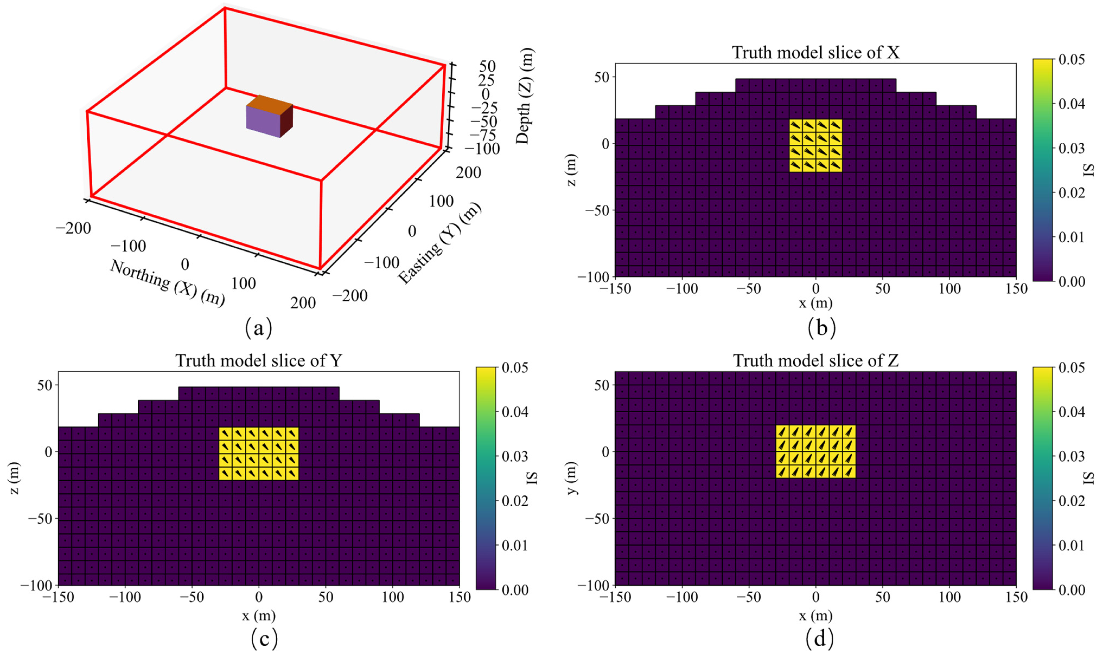
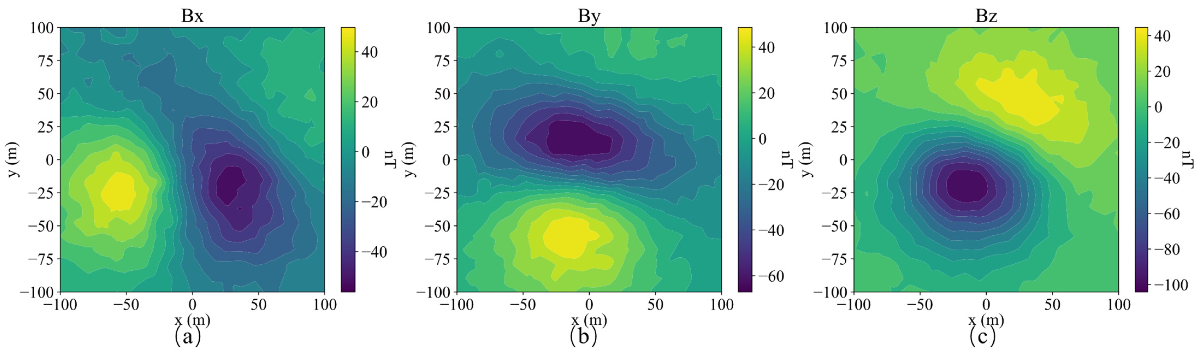
3. Inversion of Synthetic Data

To illustrate the effectiveness of the proposed algorithm, synthetic examples of two type targets will be presented in this section. The first target shown in the figure in Section 3.2 is a cuboid with the length, width, height, depth of 60 m, 40 m, and 40 m, 30 m, respectively. Its magnetic permeability is 0.05 SI. The amplitude, inclination and declination of the geomagnetic field are 50,000 nT, 90°, and 0°, respectively. The total magnetization inclination and declination of the model are 30° and 30°, respectively, and the height of the observation point from the ground is 10 m. The second target shown in the figure in Section 3.2 contains two bulk targets of the same size with magnetization inclination and declination of 30°, 30° and 60°, −45°, respectively. The observation data of the two examples are 20 × 20 grid data with 10 m intervals. The type of observational data used is three-component magnetic data with 5% of the maximum amplitude noise. The observation height is 10 m above the ground. All simulations are based on SimPEG software [42].

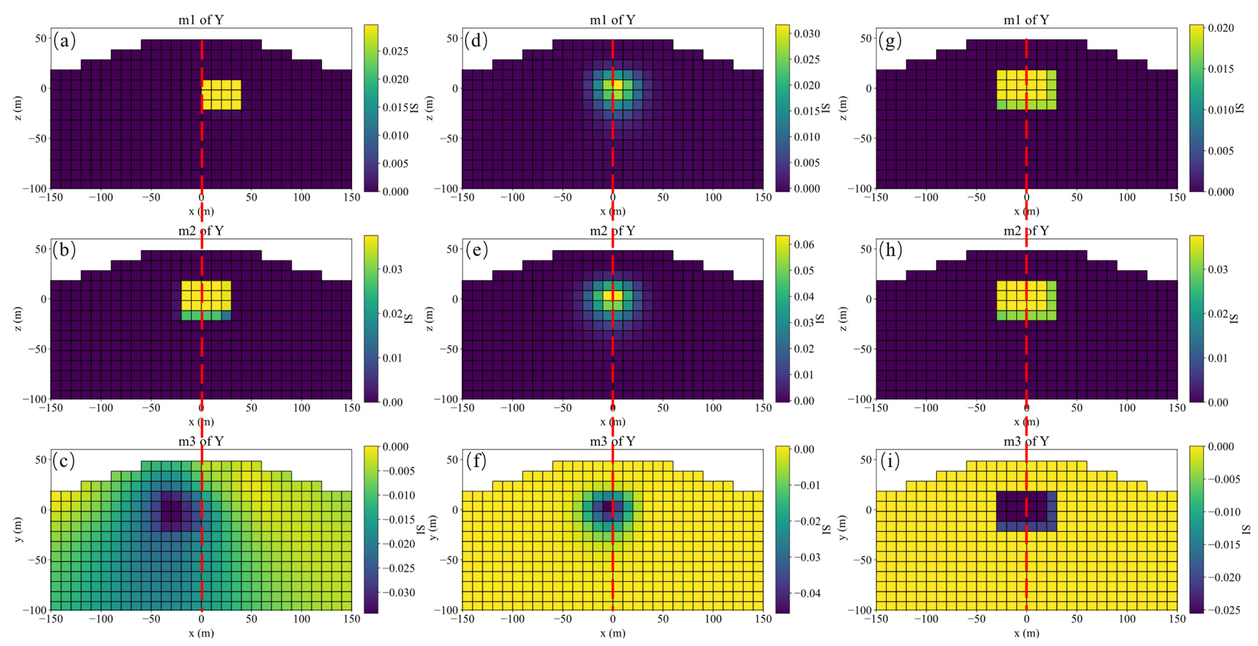
3.1. Comparison of Evaluation Effect of ${\mathcal{S}}_{RMSE}$, ${\mathcal{S}}_{IOU}$ and ${\mathcal{S}}_{IRE}$

The evaluation effects of ${\mathcal{S}}_{RMSE}$, ${\mathcal{S}}_{IOU}$ and ${\mathcal{S}}_{IRE}$ are illustrated by the following two examples. The ground truth of these two examples is a cuboid model as shown in Figure 2a–c and Figure 3a–c. The observation height is 10 m above the ground. The evaluation index comprehensively focuses on the shape, position and magnetization amplitude of the inversion result. If the above three quantities are accurate, the magnetization direction will generally be accurate.

The two inversion results of the first example are obtained under different regularization and constraint parameters. The regularization parameters $p_s$, $p_x$, $p_y$, $p_z$ of model 1 are 0, 2, 2, 2, respectively, and the model minimum term of objective function is constrained by the magnitude of the three components of magnetization. The regularization parameters $p_s$, $p_x$, $p_y$, $p_z$ of model 2 are 0, 1, 1, 1, respectively, and no amplitude constraints are imposed. The coefficients of each regularization term ${\alpha }_s$, ${\alpha }_x$, ${\alpha }_y$, ${\alpha }_z$ of two examples are both 1.0, 1.0, 1.0, 1.0, respectively. The data types are all three-component magnetic field data of Bx, By, and Bz. Figure 2a–c are slices of the ground truth, (d–f) and (g–i) are slices of the inversion model 1 and model 2, respectively. The evaluation indexes of the inversion results are shown in

Table 1. Evaluation indexes of inversion results.

Index	Model 1	Model 2	Model 3	Model 4
${\mathcal{S}}_{IOU}$	0.277	0.315	1.000	1.000
${\mathcal{S}}_{RMSE}$	0.352	0.378	0.160	0.052
${\mathcal{S}}_{IRE}$	0.789	0.834	6.255	19.108

. Observed by eyes, the inversion results of model 2 is closer to the ground truth due to the similarity in shape. It can also be reflected by the ${\mathcal{S}}_{IOU}$ value. The ${\mathcal{S}}_{IOU}$ value of model 2 is higher than that of model 1. However, the ${\mathcal{S}}_{RMSE}$ of model 1 is smaller than that of model 2, which implies that magnetization magnitude of the inversion model 1 is closer to the ground truth than model 2. This is contrary to the subjective judgment of human beings. Taking these two factors into consideration, the ${\mathcal{S}}_{IRE}$ of model 2 is greater than that of model 1, reflecting that the inversion result of model 2 is better than that of model 1, which is consistent with the human evaluation. This shows that only using ${\mathcal{S}}_{RMSE}$ as an evaluation index may lead to wrong judgments in some case.

The two inversion results of the second example are obtained by inversion of different data types. The inversion of model 3 uses total magnetization (TMI) data while model 4 uses three-component magnetic field data of Bx, By, Bz. The regularization parameters $p_s$, $p_x$, $p_y$, $p_z$ of the two models are 0, 0.8, 0.8, 0. The coefficients of each regularization term ${\alpha }_s$, ${\alpha }_x$, ${\alpha }_y$, ${\alpha }_z$ are 1.0, 0.6, 0.6, 0.2, and amplitude constraints are imposed. Figure 3a–c are slices of the ground truth, (d–f) and (g–i) are slices of the inversion model 3 and model 4, respectively. The shapes of the two inversion models are consistent with the ground truth, and the ${\mathcal{S}}_{IOU}$ values in Table 1 are also the maximum value of 1.0. At this time, it is impossible to judge which effect is better just by ${\mathcal{S}}_{IOU}$. However, the ${\mathcal{S}}_{RMSE}$ of the model 4 is smaller than that of model 3, indicating that the amplitude of the inversion model is closer to the ground truth and the inversion effect of model 4 is better. The ${\mathcal{S}}_{IRE}$ considering the shape and magnetization amplitude of model 4 is much higher than that of model 3, and it is finally judged that the inversion result of model 4 is better than that of model 3.

Combining the above two examples, there are cases where ${\mathcal{S}}_{RMSE}$ and ${\mathcal{S}}_{IOU}$ cannot evaluate the inversion effect alone. The ${\mathcal{S}}_{IRE}$ index proposed in this paper can address these two drawbacks.

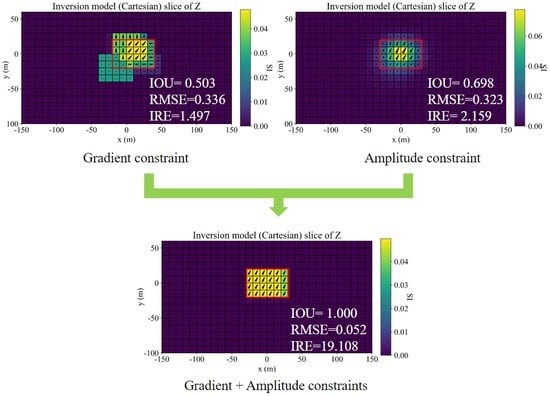
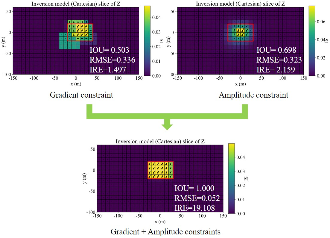
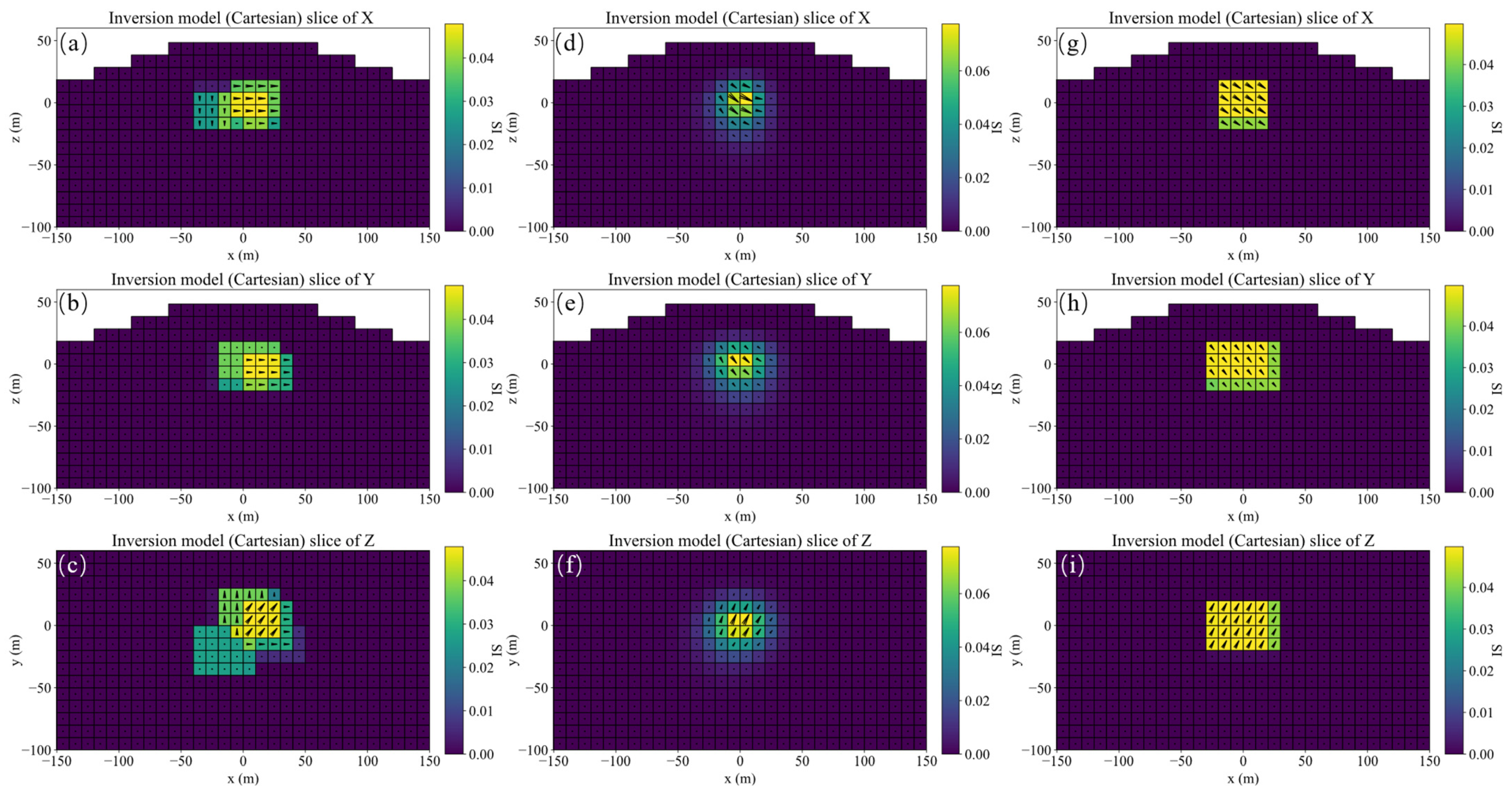
3.2. Comparison of Different Inversion Methods for Single Model

In this subsection, inversion results of three inversion methods, such as the consistency of the inversion model, the accuracy of the magnetization direction and the performance indicators proposed in this paper, are compared. Method 1 uses a traditional MVI whose objective function consists of model minimization and model gradient minimization [30] without the amplitude constraints of the three components. The objective function of method 2 only includes model minimization with the amplitude constraints of the three-component models without model gradients’ constraints. The objective function of method 3 includes model minimization and model gradient minimization with the amplitude constraints of the three-component models. The above three methods are all based on the sparse regularization framework.

The Lp norms and corresponding coefficient settings of the model minimization and model gradient minimization functions in the three Cartesian directions of the three methods are shown in the

Table 2. Regularization term coefficients and p values for the sparsity norms.

Methods	${\mathit{\alpha }}_{\mathit{s}}$	${\mathit{\alpha }}_{\mathit{x}}$	${\mathit{\alpha }}_{\mathit{y}}$	${\mathit{\alpha }}_{\mathit{z}}$	${\mathit{p}}_{\mathit{s}}$	${\mathit{p}}_{\mathit{x}}$	${\mathit{p}}_{\mathit{y}}$	${\mathit{p}}_{\mathit{z}}$
Method 1	1.0	0.6	0.6	0.2	0	0.8	0.8	0
Method 2	1.0	0	0	0	1.0	-	-	-
Method 3	1.0	0.6	0.6	0.2	0	0.8	0.8	0

. The objective function constrained by the L0 norm tends to obtain a more compact target. The larger is the norm, the more likely it is to obtain a smooth model. The smaller the value of the coefficient of the function, the stronger the constraint of the corresponding function.

A schematic diagram of single model, its slices of magnetization vector model along the X, Y, and Z directions are shown in Figure 4. The three-component observed data produced by this model are shown in Figure 5. The slices in Y direction of the three-component models inverted by method 1 shown in Figure 6a–c demonstrates that the positions of the three-component models are seriously inconsistent, which results in incoherent synthesized magnetization vector model shown in Figure 7a–c. Magnetization inclination and declination of the inversion model are shown in Figure 8a, which are far from the ground truth indicated by the red star.

The inversion results of method 2 shown in Figure 6d–f present that the position consistency of the three components has been improved compared to that of method 1. This shows that adding Lp sparsity norm constraints based on amplitude can improve the consistency of the model. However, the edge of the inversion model is not sharp, resulting in poor similarity with the ground truth, that is, poor accuracy. The synthetic magnetization vector model shown in Figure 7d–f has the same conclusion. Inverted inclination and declination shown in Figure 8b have a wide distribution range, indicating that there is still inconsistency between the three components.

The inversion results of method 3 presented in Figure 6g–i show that the positions of the three-component models are consistent, results in a synthesized model illustrated in Figure 7g–i with good consistency and integrity. Inverted inclination and declination presented in Figure 8c are consistent with the ground truth To sum up, the method proposed in this paper has the best inversion effect.

Table 3. Evaluation indexes of inversion results.

Index	Method 1	Method 2	Method 3
${\mathcal{S}}_{IOU}$	0.503	0.698	1.000
${\mathcal{S}}_{RMSE}$	0.336	0.323	0.052
${\mathcal{S}}_{IRE}$	1.497	2.159	19.108

shows the scores of the three inversion results by different evaluation indexes, including ${\mathcal{S}}_{IOU}$, ${\mathcal{S}}_{RMSE}$ and ${\mathcal{S}}_{IRE}$ proposed in this paper. For the inversion results of the three methods, the conclusions of the three evaluation indexes are the same, that is, method 3 is the best. This is consistent with the analysis of the inversion model above. In addition, the evaluation index ${\mathcal{S}}_{IRE}$ proposed in this paper has a more obvious discriminating effect compared with the other two because it has a larger span.

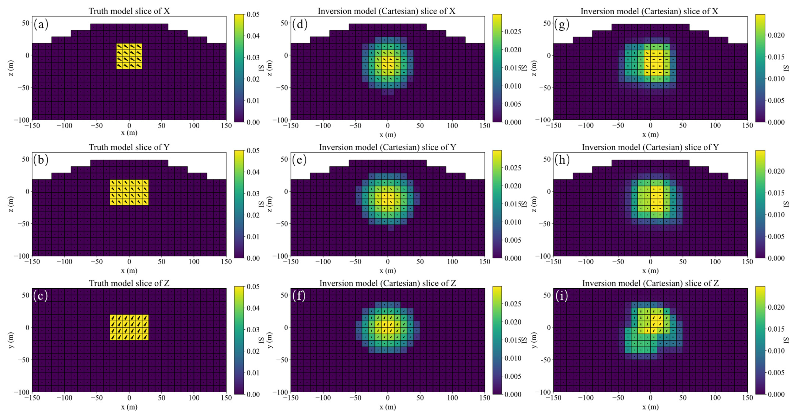
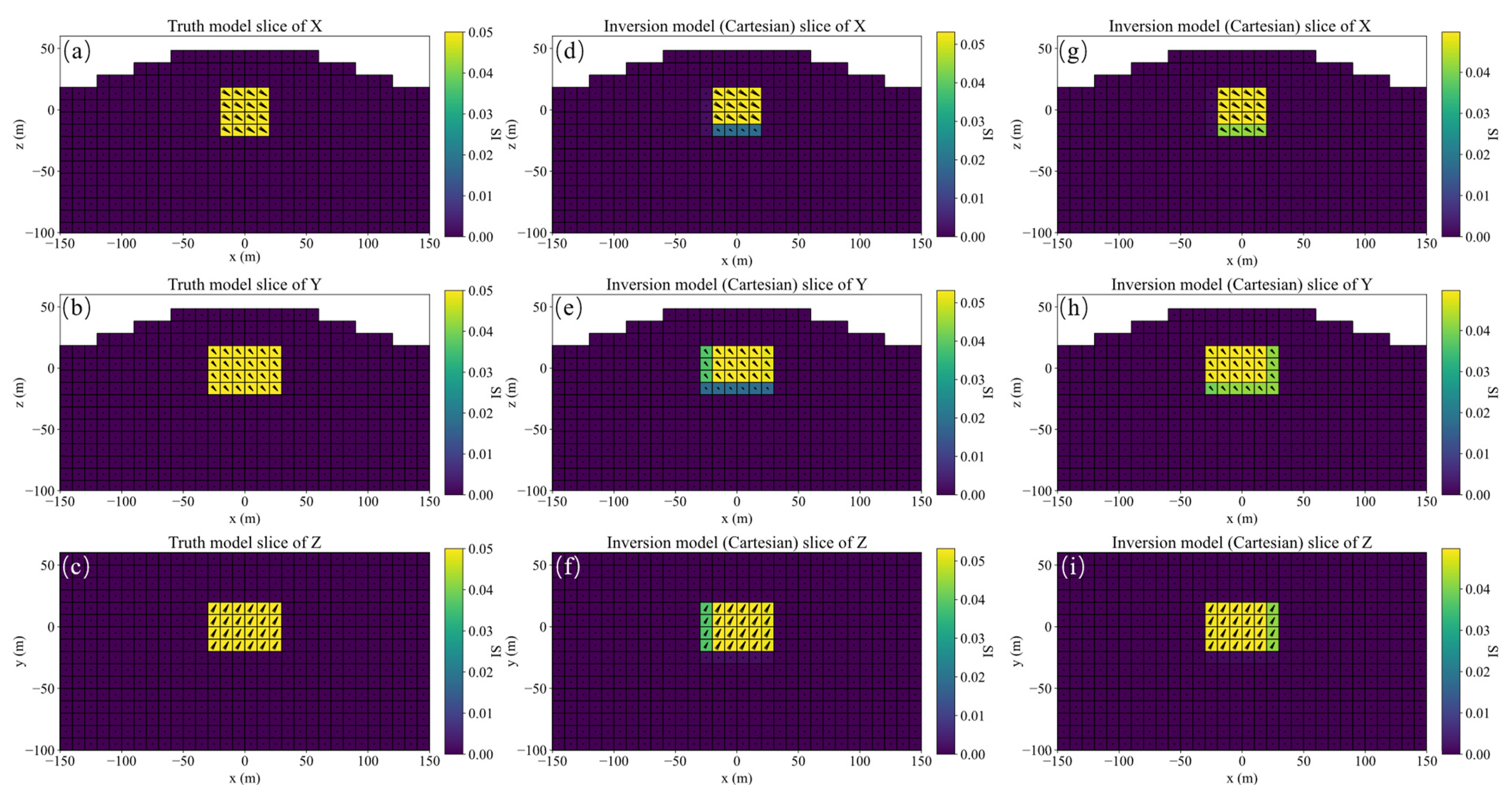
3.3. Comparison of Different Inversion Methods for Dual Models

To compare the three inversion methods in a more complex situation, the second example designs two models with inconsistent magnetization directions, as shown in Figure 8a. The magnetization declinations of two model are 30° and −45°, and magnetization inclinations are 30° and 60°, respectively. The Lp norms and corresponding coefficient settings of the model minimization and model gradients’ minimization functions in the three Cartesian directions of the three methods are shown in the

Table 4. Regularization term coefficients and p values for the sparsity norms.

Methods	${\mathit{\alpha }}_{\mathit{s}}$	${\mathit{\alpha }}_{\mathit{x}}$	${\mathit{\alpha }}_{\mathit{y}}$	${\mathit{\alpha }}_{\mathit{z}}$	${\mathit{p}}_{\mathit{s}}$	${\mathit{p}}_{\mathit{x}}$	${\mathit{p}}_{\mathit{y}}$	${\mathit{p}}_{\mathit{z}}$
Method 1	1.0	0.6	0.6	0.6	0	0.7	0.8	0
Method 2	1.0	0	0	0	1.0	-	-	-
Method 3	1.0	0.6	0.6	0.6	0	0.7	0.8	0

.

Figure 9 shows the schematic diagram of dual models, slices of magnetization vector dual models along the X, Y, and Z directions. The three-component observed data produced by dual models are shown in Figure 10. The magnetization vector models inverted by the three methods are shown in Figure 11, presenting that the inversion accuracy of method 1 is the worst, while method 3 is the best. The position and shape consistency of the model inverted by method 1 is poor. The boundary of the model inverted by method 2 is not sharp, while the model inverted by method 3 is almost completely consistent with the ground truth. This conclusion can also be shown by the polar scatter plots of magnetization inclinations and declinations as shown in Figure 12. The magnetization inclination and declination obtained by method 3 and proposed in this paper are the closest to the ground truth values (red stars) and have the highest accuracy.

Table 5. Evaluation indexes of inversion results.

Index	Method 1	Method 2	Method 3
${\mathcal{S}}_{IOU}$	0.281	0.414	1.000
${\mathcal{S}}_{RMSE}$	0.482	0.455	0.029
${\mathcal{S}}_{IRE}$	0.584	0.909	34.232

shows the scores of the three inversion results of dual models by ${\mathcal{S}}_{IOU}$, ${\mathcal{S}}_{RMSE}$ and ${\mathcal{S}}_{IRE}$. It shows that the inversion effect by the method proposed in this paper is best. The conclusions drawn from the evaluation indexes are consistent with the results observed by the inversion model.

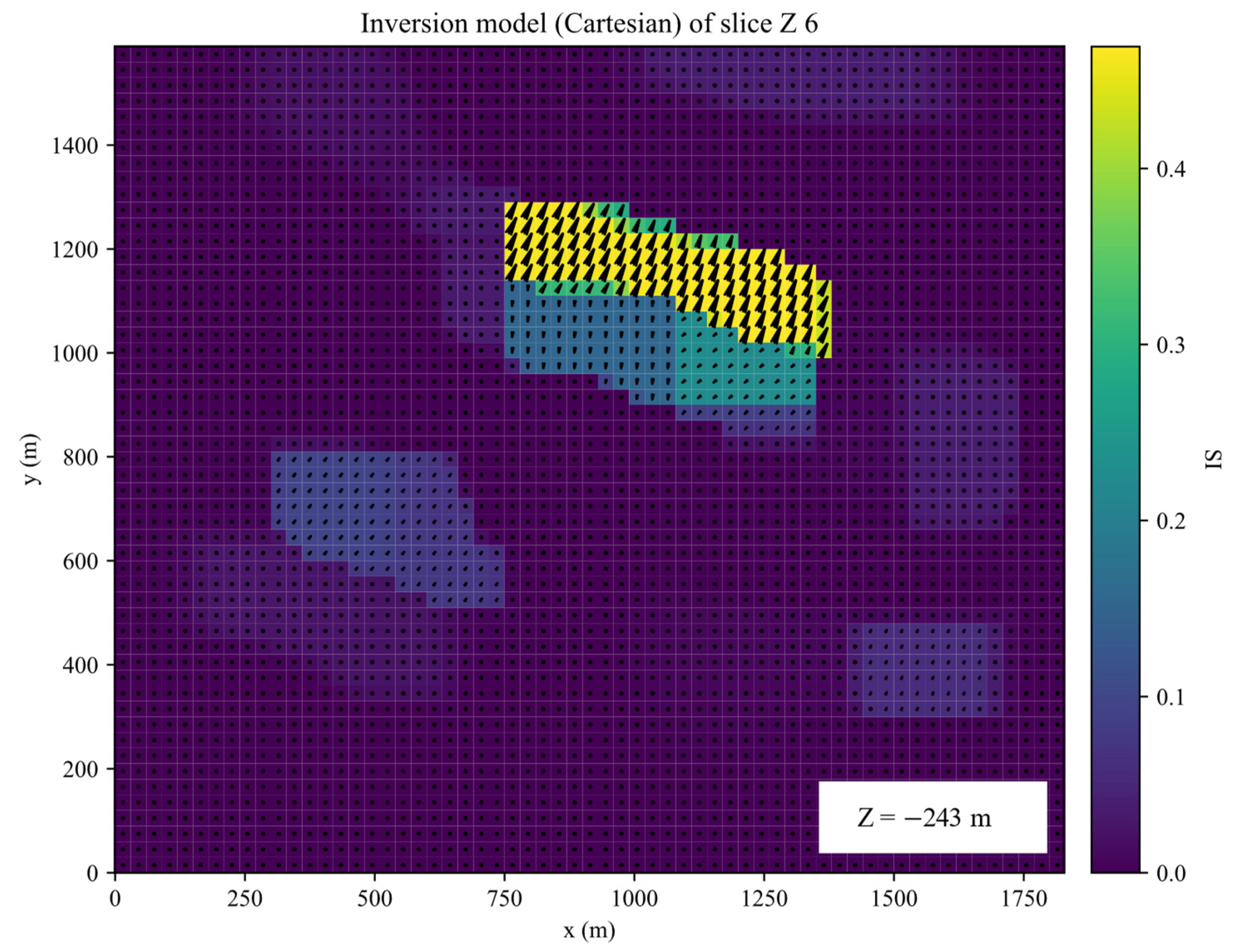
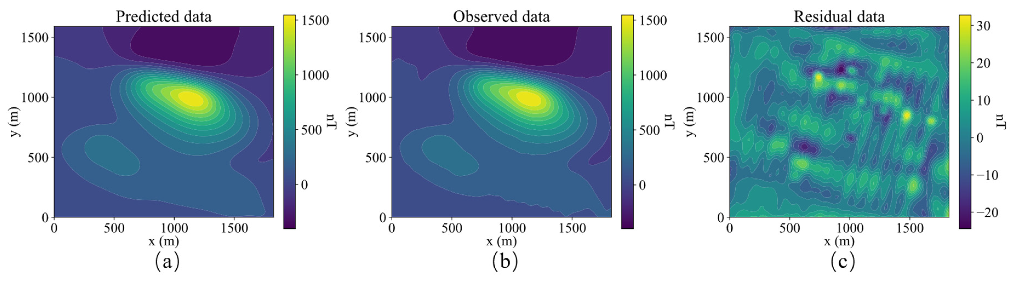
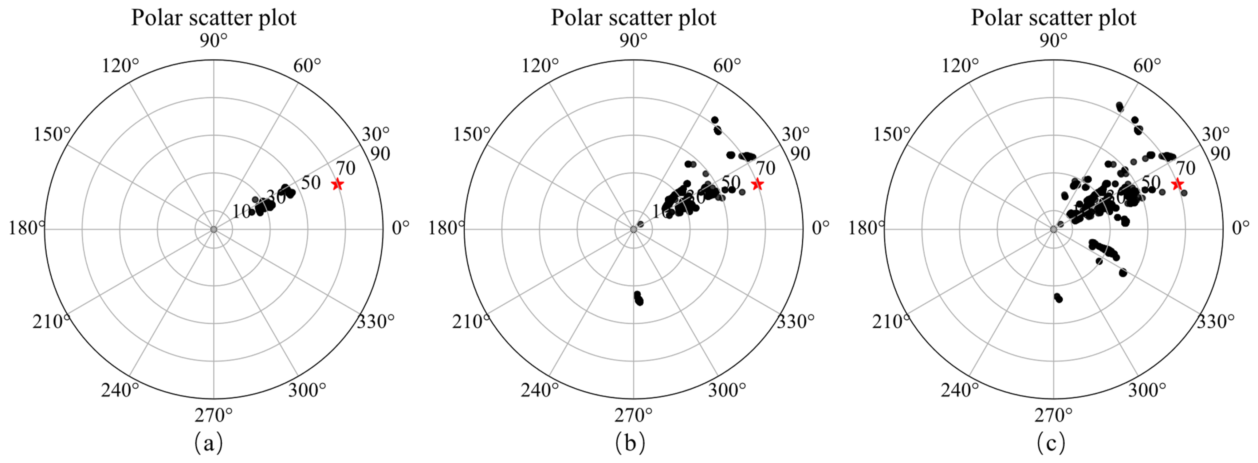
4. Inversion of Real Data

In this study, real measured data of Galinge iron ore deposit located at the center of Qimantage metallogenic belt in Qinghai province (NW China) is used to verify the effectiveness of proposed method. For detailed information about the Galinge iron ore deposit, please refer to the papers [17].

The observation range of Galinge iron ore deposit is 1827 m in the east-west direction with a total of 100 points, and 1589.7 m in the north-south direction with a total of 87 points. Underground is divided into prismatic grids with sides of 30 m. The observation height is about 2 m, and the local geomagnetic inclination and declination are 50° and −4°, respectively. The norms of model minimization and model gradient minimization in x, y, and z directions are 0, 0.8, 0.8 and 0, respectively, and the corresponding coefficients of the corresponding functions are 1.0, 1.0, 1.0, and 1.0, respectively.

The inversion was performed for 35 iterations. The inverted results of slices along the X, Y, Z planes of inverted Galinge iron ore deposit are shown in the Figure 13, Figure 14, Figure 15 and Figure 16. They present that the shape, location, and magnitude of the inversion are similar to that in those papers [17,32].

Figure 17 shows contour plots of the predicted data by the inverted model, observed data and residual data. The predicted data is very close to the observed data, with a residual of around 30 nT.

Figure 18 shows the polar scatter plots of inverted magnetization inclination and declination with large, medium, and small cutoff values. When a large cutoff value is applied, the average value of inverted magnetization declination is 25°, as shown by the regions with large magnetization amplitudes in Figure 11. There are two distinct magnetization inclinations, around 30° and 45°. When the cutoff value becomes smaller, the magnetization direction of more regions can be displayed.

5. Conclusions

In this study, a magnetization vector inversion method where the model and its three Cartesian gradients are simultaneously constrained by the sparse Lp norm based on the magnitude of the three-component models is proposed. This method can obtain a more consistent and sharper model by adjusting the norm and the corresponding coefficient of the sparse constraints. In addition, to better evaluate the inversion effect, this paper proposes a new evaluation index ${\mathcal{S}}_{IRE}$ that combines ${\mathcal{S}}_{RMSE}$ and ${\mathcal{S}}_{IOU}$, which solves the problem that ${\mathcal{S}}_{RMSE}$ and ${\mathcal{S}}_{IOU}$ alone cannot accurately evaluate the inversion results. According to synthetic examples of single and dual models, the methods proposed in this paper have a superior inversion accuracy, which can be reflected by the inversion model and the evaluation indexes. This method solves the inconsistency of the inversion in the Cartesian coordinate system and obtains inversion models with good edge accuracy. The model inverted from the measured Galinge iron ore deposit (China) data is consistent with the real geological information. This method has great potential to be applied to scenarios that require high inversion accuracy, such as the inversion of small objects, but the inversion of deeper objects still needs further research.

References

1. Nabighian, M.N.; Grauch, V.J.S.; Hansen, R.O.; LaFehr, T.R.; Li, Y.; Peirce, J.W.; Phillips, J.D.; Ruder, M.E. The historical development of the magnetic method in exploration. Geophysics 2005, 70, 33ND–61ND. [Google Scholar] [CrossRef]
2. Wang, C.; Shi, W.; Zhu, J.; Xu, J.; Chen, S.; Li, Y. Prospecting of sedimentary-metamorphic type manganese deposits in the Sifangshan area northeastern Hubei Province: Insight from magnetic anomaly information. Bull. Geol. Sci. Technol. 2022, 41, 84–196. [Google Scholar]
3. Tao, G.; Wang, G.; Zhang, Z. Extraction of mineralization-related anomalies from gravity and magnetic potential fields for mineral exploration targeting: Tongling Cu (–Au) District, China. Nat. Resour. Res. 2019, 28, 461–486. [Google Scholar] [CrossRef]
4. Lin, C.S.; Zhou, J.J.; Yang, Z.Y. A method to solve the aircraft magnetic field model basing on geomagnetic environment simulation. J. Magn. Magn. Mater. 2015, 384, 314–319. [Google Scholar] [CrossRef]
5. Yin, G.; Zhang, Y.T.; Li, Z.N.; Fan, H.B.; Ren, G.Q. Detection of ferromagnetic target based on mobile magnetic gradient tensor system. J. Magn. Magn. Mater. 2016, 402, 1–7. [Google Scholar]
6. Guo, Z.Y.; Liu, D.J.; Pan, Q.; Zhang, Y.Y. Forward modeling of total magnetic anomaly over a pseudo-2D underground ferromagnetic pipeline. J. Appl. Geophys. 2015, 113, 14–30. [Google Scholar] [CrossRef]
7. Hu, Z.; Lü, B.; Du, J.; Sun, S.; Chen, C. Application of Susceptibility Imaging Method by Minimum⁃Structure Inversion to Underwater Target Detection. Earth Sci. 2021, 46, 3376–3384. [Google Scholar]
8. Davis, K.; Li, Y.; Nabighian, M. Automatic detection of UXO magnetic anomalies using extended Euler deconvolution. Geophysics 2010, 3, G13–G20. [Google Scholar] [CrossRef]
9. Chen, H.L.; Wang, C.L.; Zuo, X.Z. Research on methods of defect classification based on metal magnetic memory. NDT E Int. 2017, 92, 82–87. [Google Scholar] [CrossRef]
10. Yin, G.; Zhang, L. Three-dimensional reconstruction of a small-scale magnetic target from magnetic gradient observations. J. Magn. Magn. Mater. 2019, 482, 229–238. [Google Scholar] [CrossRef]
11. Sharma, P.V. Rapid computation of magnetic anomalies and demagnetization effects caused by bodies of arbitrary shape. Pure Appl. Geophys. 1966, 64, 89–109. [Google Scholar] [CrossRef]
12. Plouff, D. Gravity and magnetic fields of polygonal prisms and application to magnetic terrain corrections. Geophysics 1976, 41, 727–741. [Google Scholar] [CrossRef]
13. Guo, Z.H.; Guan, Z.N.; Xiong, S.Q. Cuboid ∆T and its gradient forward theoretical expressions without analytic odd points. Chin. J. Geophys. 2004, 47, 1131–1138. (In Chinese) [Google Scholar] [CrossRef]
14. Ren, Z.; Zhang, Y.; Zhong, Y.; Pan, K.; Wu, Q.; Tang, J. Magnetic anomalies caused by 3D polyhedral structures with arbitrary polynomial magnetization. Geophys. Res. Lett. 2022, 19, e2022GL099209. [Google Scholar] [CrossRef]
15. Ellis, R.G.; de Wet, B.; Macleod, I.N. Inversion of magnetic data for remanent and induced sources. ASEG Ext. Abstr. 2012, 2012, 1–4. [Google Scholar]
16. Clark, D.A. Methods for determining remanent and total magnetizations of magnetic sources—A review. Explor. Geophys. 2014, 45, 271–304. [Google Scholar] [CrossRef]
17. Liu, S.; Hu, X.; Zhang, H.; Geng, M.; Zuo, B. 3D magnetization vector inversion of magnetic data: Improving and comparing methods. Pure Appl. Geophys. 2017, 174, 4421–4444. [Google Scholar] [CrossRef]
18. Li, Y.; Shearer, S.E.; Haney, M.M.; Dannemiller, N. Comprehensive approaches to 3D inversion of magnetic data affected by remanent magnetization. Geophysics 2010, 75, L1–L11. [Google Scholar] [CrossRef]
19. Lourenco, J.S.; Morrison, H.F. Vector magnetic anomalies derived from measurements of a single component of the field. Geophysics 1973, 38, 359–368. [Google Scholar] [CrossRef]
20. Rezaie, M. 3D Inversion of Magnetic Amplitude Data with Sparseness Constraint. Pure Appl. Geophys. 2021, 178, 2111–2126. [Google Scholar] [CrossRef]
21. Shearer, S.; Li, Y. 3D inversion of magnetic total gradient data in the presence of remanent magnetization. In Proceedings of the Society of Exploration Geophysicists, Denver, CO, USA, 10–15 October 2004. [Google Scholar]
22. Gubbins, D.; Ivers, D.; Williams, S. Analysis of Crustal Magnetisation in Cartesian Vector Harmonics. In Proceedings of the AGU Fall Meeting Abstracts, San Franisco, CA, USA, 14–18 December 2015. [Google Scholar]
23. Li, Y.; Oldenburg, D.W. 3-D inversion of gravity data. Geophysics 1998, 63, 109–119. [Google Scholar] [CrossRef]
24. Parker, R.L.; Shure, L.; Hildebrand, J.A. The application of inverse theory to seamount magnetism. Rev. Geophys. 1987, 25, 17–40. [Google Scholar] [CrossRef]
25. Wang, M.; Di, Q.; Xu, K.; Wang, R. Magnetic vector inversion equations and forward and inversed 2d model study. Chin. J. Geophys. 2004, 47, 601–609. [Google Scholar] [CrossRef]
26. Lelièvre, P.G.; Oldenburg, D.W. A 3D total magnetization inversion applicable when significant, complicated remanence is present. Geophysics 2009, 74, L21–L30. [Google Scholar] [CrossRef]
27. Liu, S.; Hu, X.; Liu, T.; Feng, J.; Gao, W.; Qiu, L. Magnetization vector imaging for borehole magnetic data based on magnitude magnetic anomaly. Geophysics 2013, 78, D429–D444. [Google Scholar] [CrossRef]
28. Zhu, Y.; Hdanov, M.S.; Cuma, M. Inversion of TMI data for the magnetization vector using Gramian constraints. In Proceedings of the 85th Annual International Meeting, Tulsa, OK, USA, 1 July 2015. [Google Scholar]
29. Li, Y.; Sun, J. 3D magnetization inversion using fuzzy c-means clustering with application to geology differentiation. Geophysics 2016, 81, J61–J78. [Google Scholar] [CrossRef]
30. Fournier, D.; Oldenburg, D.W. Inversion using spatially variable mixed ℓ p norms. Geophys. J. Int. 2019, 218, 268–282. [Google Scholar] [CrossRef]
31. Fournier, D. Advanced Potential Field Data Inversion with Lp-Norm Regularization. Ph.D. Dissertation, British Columbia University, Vancouver, CA, Canada, 2019. [Google Scholar]
32. Ghalehnoee, M.H.; Ansari, A. Compact magnetization vector inversion. Geophys. J. Int. 2022, 228, 1–16. [Google Scholar] [CrossRef]
33. Liu, B.; Guo, Q.; Li, S.; Liu, B.; Ren, Y.; Pang, Y.; Guo, X.; Liu, L.; Jiang, P. Deep Learning Inversion of Electrical Resistivity Data. IEEE Trans. Geosci. Remote Sens. 2020, 58, 5715–5728. [Google Scholar] [CrossRef] [Green Version]
34. Hu, Z.; Liu, S.; Hu, X.; Fu, L.; Qu, J.; Wang, H.; Chen, Q. Inversion of magnetic data using deep neural networks. Phys. Earth Planet. Inter. 2021, 311, 106653. [Google Scholar] [CrossRef]
35. Vatankhah, S.; Liu, S.; Renaut, R.A.; Hu, X.; Hogue, J.D.; Gharloghi, M. An Efficient Alternating Algorithm for the Lₚ-Norm Cross-Gradient Joint Inversion of Gravity and Magnetic Data Using the 2-D Fast Fourier Transform. IEEE Trans. Geosci. Remote Sens. 2020, 60, 4500416. [Google Scholar]
36. Li, Y.; Oldenburg, D.W. 3-D inversion of magnetic data. Geophysics 1998, 61, 394–408. [Google Scholar] [CrossRef]
37. Lawson, C.L. Contribution to the Theory of Linear Least Maximum Approximation. Ph.D. Dissertation, California University, Los Angeles, CA, USA, 1961. [Google Scholar]
38. Vatankhah, S.; Renaut, R.A.; Liu, S. Research note: A unifying framework for the widely used stabilization of potential field inverse problems. Geophy. Prospect. 2020, 68, 1416–1421. [Google Scholar] [CrossRef]
39. Zhou, D.; Fang, J.; Song, X.; Guan, C.; Yin, J.; Dai, Y.; Yang, R. Iou loss for 2d/3d object detection. In Proceedings of the 2019 International Conference on 3D Vision (3DV), Quebec City, QC, Canada, 16–19 September 2019. [Google Scholar]
40. Cheng, B.; Girshick, R.; Dollár, P.; Berg, A.C.; Kirillov, A. Boundary IoU: Improving object-centric image segmentation evaluation. In Proceedings of the IEEE/CVF Conference on Computer Vision and Pattern Recognition, Nashville, TN, USA, 20–25 June 2021. [Google Scholar]
41. Rezatofighi, H.; Tsoi, N.; Gwak, J.; Sadeghian, A.; Reid, I.; Savarese, S. Generalized Intersection Over Union: A Metric and a Loss for Bounding Box Regression. In Proceedings of the 2019 IEEE/CVF Conference on Computer Vision and Pattern Recognition (CVPR), Long Beach, CA, USA, 15–20 June 2019. [Google Scholar]
42. Cockett, R.; Kang, S.; Heagy, L.J.; Pidlisecky, A.; Oldenburg, D.W. SimPEG: An open source framework for simulation and gradient based parameter estimation in geophysical applications. Comput. Geosci. 2015, 85, 142–154. [Google Scholar] [CrossRef]
Figure 1. Inversion process based on the method proposed in this paper.
Remotesensing 14 05497 g001
Figure 2. Slices in three Cartesian directions of the ground truth (ac) and inverted model 1 (df) and model 2 (gi) under different regularization and constraint parameters, respectively.
Remotesensing 14 05497 g002
Figure 3. Slices in three Cartesian directions of the ground truth (ac), inverted model 3 (df) and model 4 (gi) under different data types of TMI and three-component magnetic field data, respectively.
Remotesensing 14 05497 g003
Figure 4. (a) Schematic diagram of a single model; Slices of magnetization vector model along the X (b), Y (c), and Z (d) directions.
Remotesensing 14 05497 g004
Figure 5. Three-component observed data Bx (a), By (b) and Bz (c) of a single model.
Remotesensing 14 05497 g005
Figure 6. Y slices of the three-component magnetization models inverted by method 1 (ac), method 2 (df) and method 3 (gi), respectively.
Remotesensing 14 05497 g006
Figure 7. Slices along the X, Y, and Z directions of the magnetization vector models inverted by method 1 (ac), method 2 (df), and method 3 (gi), respectively.
Remotesensing 14 05497 g007
Figure 8. Polar scatter plots showing inverted magnetic inclination (radial) and declination (axial) of method 1 (a), method 2 (b) and method 3 (c) and the ground truth (red star).
Remotesensing 14 05497 g008
Figure 9. (a) Schematic diagram of dual models; slices of magnetization vector dual models along the X (b), Y (c), and Z (d) directions.
Remotesensing 14 05497 g009
Figure 10. Three-component observation data of Bx (a), By (b), Bz (c) of the dual model.
Remotesensing 14 05497 g010
Figure 11. Slices along the X, Y, and Z directions of the magnetization vector models inverted by method 1 (ac), method 2 (df), and method 3 (gi), respectively.
Remotesensing 14 05497 g011
Figure 12. Polar scatter plots showing inverted magnetic inclination (radial) and declination (axial) of method 1 (a), method 2 (b) and method 3 (c) and the ground truth (red stars).
Remotesensing 14 05497 g012
Figure 13. Slices along the X planes of inverted Galinge iron ore deposit.
Remotesensing 14 05497 g013
Figure 14. Slices along the Y planes of inverted Galinge iron ore deposit.
Remotesensing 14 05497 g014
Figure 15. Slices along the Z planes of inverted Galinge iron ore deposit.
Remotesensing 14 05497 g015
Figure 16. Slices along the Z planes of inverted Galinge iron ore deposit.
Remotesensing 14 05497 g016
Figure 17. Contour plots of predicted data (a), observed data (b) and residual data (c).
Remotesensing 14 05497 g017
Figure 18. Polar scatter plots showing inverted magnetic inclination (radial) and declination (axial) with large (a), medium (b), and small (c) cutoff values and the result of Liu [17] in red star.
Remotesensing 14 05497 g018