

An Empirical Correction Model for Remote Sensing Data of Global Horizontal Irradiance in High-Cloudiness-Index Locations


Abstract
:1. Introduction
1.1. State of the Art
1.2. Ecuadorian Context as a Case Study
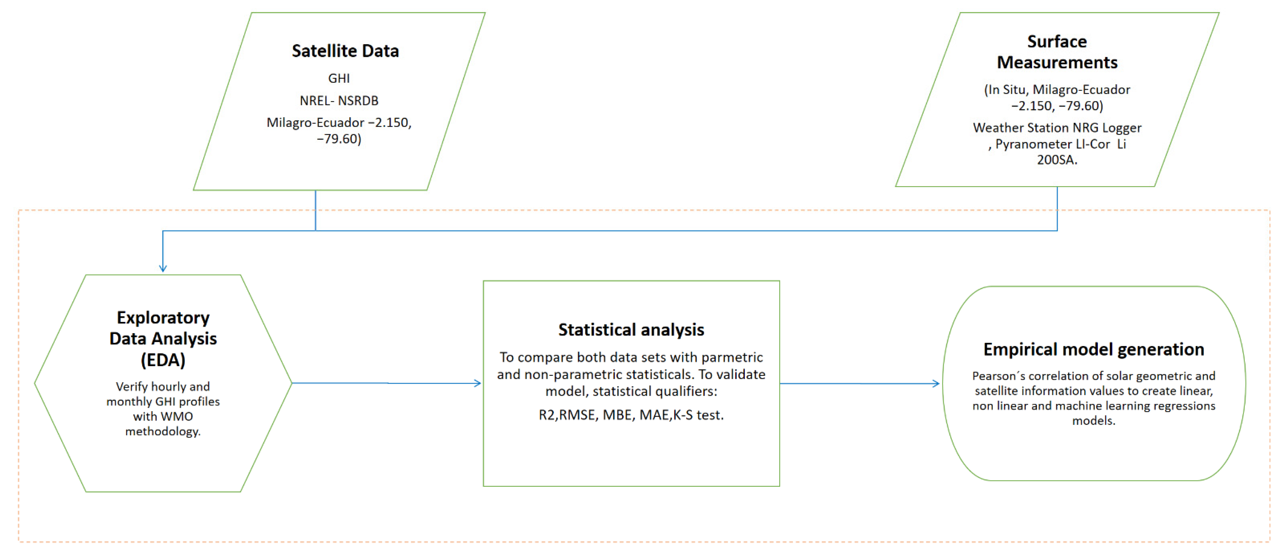
2. Materials and Methods
2.1. Surface Measurement Set Up
2.2. Data Processing
- Physically possible limits;
- Extremely rare limits;
- Compared to each other (direct and diffuse irradiance).
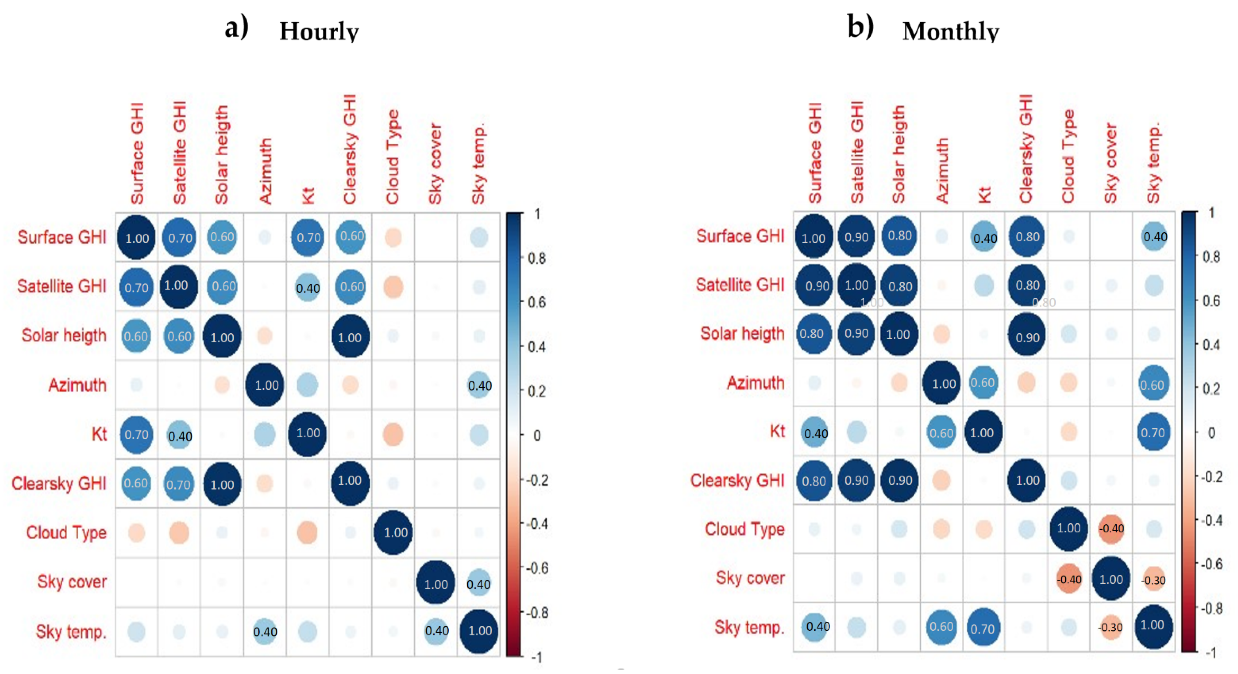
2.3. Parametric and Non-Parametric Satellite GHI Validation
2.4. Site-Adaptation, Definition of Input Parameters
Correlation Analysis
2.5. Satellite GHI Fit Model Generation
2.5.1. Application of Linear, Non-Linear Regressions and Machine Learning
- A null model M0 with no predictors is generated.
- Then, M1 models containing only one predictor are generated and the best one is selected.
- The previous process is repeated for models containing two variables and so on until the n predictor variables are completed.
- From among all the models (M0,M1,M2,…Mn), the best one is selected through cross validation, which for this study will be the adjusted R2.
2.6. Selection and Evaluation of the Optimal Model
3. Results
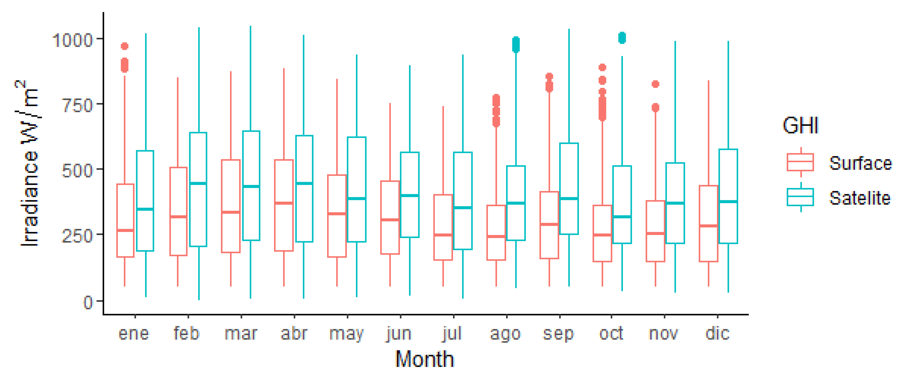
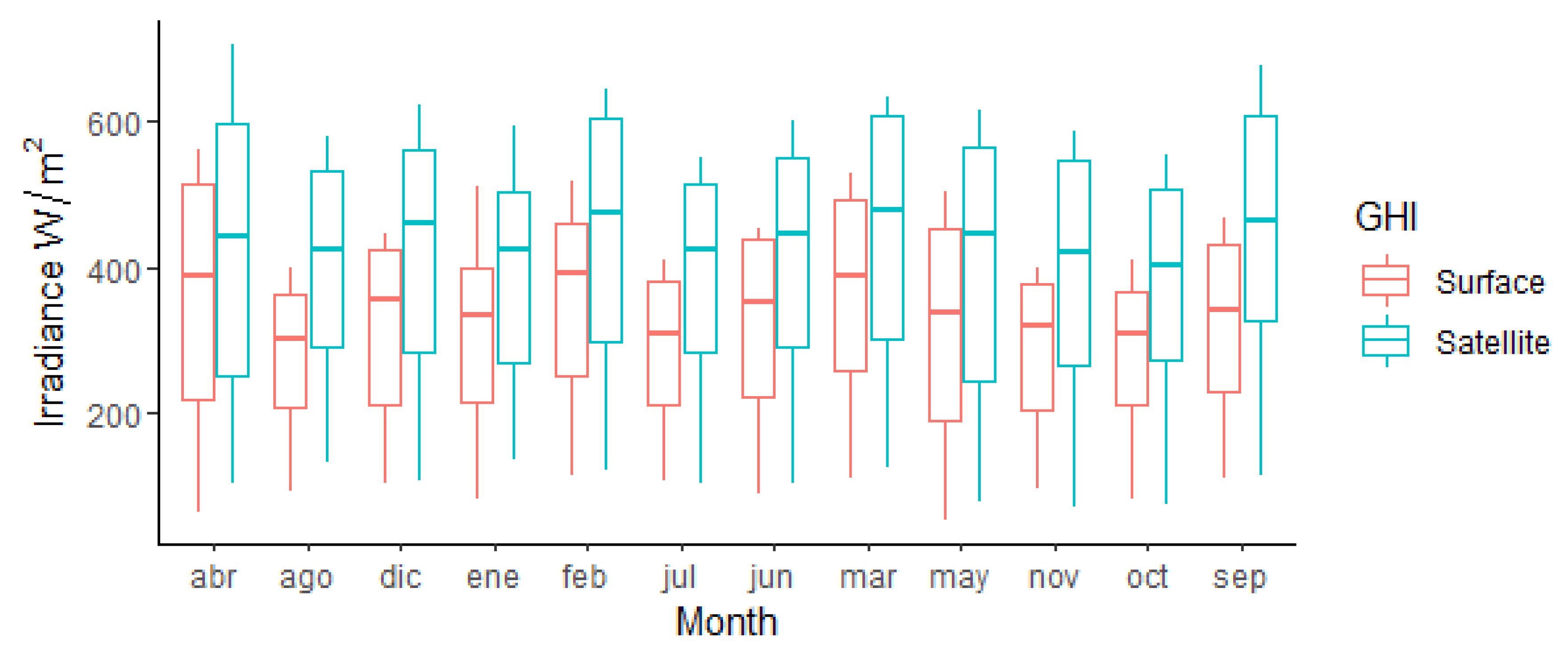
3.1. Verification
3.2. Validation
3.3. Site-Adaptation and Cloudiness Model
3.4. Selection and Evaluation of the Optimal Cloudiness Model
4. Discussion
5. Conclusions
- The validation of the satellite GHI from the NREL database considered a parametric and non-parametric analysis. The parametric linearity analysis showed a linear trend for the hourly and monthly GHI profiles considered. The hourly profile had a lower R2 compared to the R2 of the monthly profile.
- A comparison of medians between the surface GHI data series versus the satellite GHI data series showed an overestimation of the solar resource in the satellite GHI.
- The parametric normality tests showed that the hourly and monthly profiles evaluated did not satisfy the defined parameters; therefore, a non-parametric validation analysis was necessary.
- The parametric variance of the residuals test revealed that only the monthly profile complied with homoscedasticity.
- Parametric tests for influential points revealed in both the hourly and monthly GHI profiles the absence of outliers or anomalous values that could have an impact on the prediction model.
- Non-parametric and dispersion statistics analysis identified the hourly profile as inapplicable for simulation purposes. From the hourly profile, the site-adaptation process was performed.
Author Contributions
Funding
Data Availability Statement
Acknowledgments
Conflicts of Interest
Abbreviations
| AS | All Sky |
| CAMS | Copernicus Atmosphere Monitoring Service |
| CIM | Cloud Index Method |
| COP26 | Conference of the Parties |
| CSI | Clear Sky |
| DNI | Direct Normal Irradiance |
| DS | Cloudy Sky |
| FARMS | Fast All-sky Radiation Model for Solar applications |
| GHI | Global Horizontal Irradiation [W m2] |
| GOES | Geostationary Operational Environmental Satellites |
| GLMNET | Elastic Net regression |
| INHAMI | National Institute of Meteorology and Hydrology |
| KS-test | Kolmogorov–Smirnov test |
| Kt | Clearness Index |
| MARS | Multivariate Adaptive Regression Splines |
| MBE | Mean Bias Error |
| MOS | Model Output Statistics |
| NREL | National Renewable Energy Laboratory |
| NSRDB | National Solar Radiation Database |
| ODR | Orthogonal Distance Regression |
| PSM | Physical Solar Model |
| RF | Random Forests |
| RMSE | Root Mean Square Error |
| SCSI | Semi-Clear Sky |
| SDE | Stochastic Differential Equation |
| SDR | Symphonie Data Retriever |
| SVR | Support Vector Regression |
| UNEMI | State University of Milagro |
| WMO | World Meteorological Organization |
| WRF | Weather and Research Forecasting |
| XGBoost | Extreme Gradient Boosting Machines |
References
- Masson-Delmotte, V.; Zhai, P.; Pirani, A.; Connors, S.L.; Péan, C.; Berger, S.; Caud, N.; Chen, Y.; Goldfarb, L.; Gomis, M.I.; et al. IPCC 2021: Climate Change 2021: The Physical Science Basis. Contribution of Working Group I to the Sixth Assessment Report of the Intergovernmental Panel on Climate Change; Cambridge University Press: Cambridge, UK, 2021; in press; Available online: https://www.ipcc.ch/report/ar6/wg1/ (accessed on 22 April 2022).
- COP26|Naciones Unidas. Available online: https://www.un.org/es/climatechange/cop26 (accessed on 22 April 2022).
- NREL. NSRDB Data Viewer. 2022. Available online: https://nsrdb.nrel.gov/data-viewer (accessed on 15 January 2022).
- Perez, R.; David, M.; Hoff, T.E.; Jamaly, M.; Kivalov, S.; Kleissl, J.; Lauret, P.; Perez, M. Spatial and temporal variability of solar energy. Found. Trends® Renew. Energy 2016, 1, 1–44. [Google Scholar] [CrossRef] [Green Version]
- Sengupta, M.; Habte, A.; Wilbert, S.; Gueymard, C.; Remund, J. Best Practices Handbook for the Collection and Use of Solar Resource Data for Solar Energy Applications, 3rd ed.; NREL/TP-5D00-63112; National Renewable Energy Laboratory: Denver, CO, USA, 2021. Available online: https://www.nrel.gov/docs/fy15osti/63112.pdf (accessed on 1 September 2022).
- Badosa, J.; Gobet, E.; Grangereau, M.; Kim, D. Day-ahead probabilistic forecast of solar irradiance: A stochastic differential equation approach. Springer Proc. Math. Stat. 2018, 254, 73–93. [Google Scholar] [CrossRef] [Green Version]
- Polo, J.; Wilbert, S.; Ruiz-Arias, J.; Meyer, R.; Gueymard, C.; Súri, M.; Martín, L.; Mieslinger, T.; Blanc, P.; Grant, I.; et al. Preliminary survey on site-adaptation techniques for satellite-derived and reanalysis solar radiation datasets. Sol. Energy 2016, 132, 25–37. [Google Scholar] [CrossRef]
- Fernández-Peruchena, C.M.; Polo, J.; Martín, L.; Mazorra, L. Site-adaptation of modeled solar radiation data: The SiteAdapt procedure. Remote Sens. 2020, 12, 2127. [Google Scholar] [CrossRef]
- Polo, J.; Fernández-Peruchena, C.; Salamalikis, V.; Mazorra-Aguiar, L.; Turpin, M.; Martín-Pomares, L.; Kazantzidis, A.; Blanc, P.; Remund, J. Benchmarking on improvement and site-adaptation techniques for modeled solar radiation datasets. Sol. Energy 2020, 201, 469–479. [Google Scholar] [CrossRef]
- Vamvakas, I.; Salamalikis, V.; Benitez, D.; Al-Salaymeh, A.; Bouaichaoui, S.; Yassaa, N.; Guizani, A.; Kazantzidis, A. Estimation of global horizontal irradiance using satellite-derived data across Middle East-North Africa: The role of aerosol optical properties and site-adaptation methodologies. Renew. Energy 2020, 157, 312–331. [Google Scholar] [CrossRef]
- Cucumo, M.; Kaliakatsos, D.; Marinelli, V. A calculation method for the estimation of the Linke turbidity factor. Renew. Energy 2000, 19, 249–258. [Google Scholar] [CrossRef]
- Cebecauer, T.; Suri, M. Site-adaptation of satellite-based DNI and GHI time series: Overview and SolarGIS approach. AIP Conf. Proc. 2016, 1734, 150002. [Google Scholar] [CrossRef] [Green Version]
- Fernández-Peruchena, C.M.; Bernardos, A.; Gastón, M.; Gonzalez, R. Estimación de recurso solar a largo plazo para aplicaciones energéticas solares. In Proceedings of the XVI Congreso Ibérico y XII Congreso Iberoamericano de Energía Solar, Madrid, Spain, 20–22 June 2018; Available online: https://hal.archives-ouvertes.fr/hal-02380032 (accessed on 1 September 2022).
- Rincón, A.; Jorba, O.; Frutos, M.; Alvarez, L.; Barrios, F.P.; González, J.A. Bias correction of global irradiance modelled with weather and research forecasting model over Paraguay. Sol. Energy 2018, 170, 201–211. [Google Scholar] [CrossRef]
- Frank, C.W.; Wahl, S.; Keller, J.D.; Pospichal, B.; Hense, A.; Crewell, S. Bias correction of a novel European reanalysis data set for solar energy applications. Sol. Energy 2018, 164, 12–24. [Google Scholar] [CrossRef]
- Narvaez, G.; Giraldo, L.F.; Bressan, M.; Pantoja, A. Machine learning for site-adaptation and solar radiation forecasting. Renew. Energy 2021, 167, 333–342. [Google Scholar] [CrossRef]
- Laguarda, A.; Giacosa, G.; Alonso-Suárez, R.; Abal, G. Performance of the site-adapted CAMS database and locally adjusted cloud index models for estimating global solar horizontal irradiation over the Pampa Húmeda. Sol. Energy 2020, 199, 295–307. [Google Scholar] [CrossRef]
- Salamalikis, V.; Tzoumanikas, P.; Argiriou, A.A.; Kazantzidis, A. Site adaptation of global horizontal irradiance from the Copernicus Atmospheric Monitoring Service for radiation using supervised machine learning techniques. Renew. Energy 2022, 195, 92–106. [Google Scholar] [CrossRef]
- Berrones, G.; Crespo, P.; Ochoa-Sánchez, A.; Wilcox, B.P.; Célleri, R. Importance of fog and cloud water contributions to soil moisture in the Andean Páramo. Hydrology 2022, 9, 54. [Google Scholar] [CrossRef]
- Agencia de Regulación y Control de Energía y Recursos Naturales no Renovables, “Plan Anual de Operación Estadística Pao 2022 Dirección de Estudios e Información del Sector Eléctrico. 2022. Available online: https://www.controlrecursosyenergia.gob.ec/wp-content/uploads/downloads/2021/09/PAO2022-firmado.pdf (accessed on 20 January 2022).
- CONELEC. Atlas Solar del Ecuador; Conelec: Quito, Ecuador, 2008; pp. 1–51. Available online: http://www.conelec.gob.ec/archivos_articulo/Atlas.pdf (accessed on 20 January 2022).
- MEER. Atlas Eólico. 2013. Available online: https://es.scribd.com/document/355204005/ATLAS-EOLICO-ECUADOR-MEER-2013-pdf (accessed on 20 January 2022).
- Ecuador Instituto Nacional de Preinversión; Ministerio de Electricidad y Energía Renovable; Ministerio Coordinador de Producción, Empleo y Competitividad. Atlas Biometrico del Ecuador; Ecuador; Instituto Nacional de Preinversión: Quito, Equador, 2014; p. 156. [Google Scholar]
- Cevallos-Sierra, J.; Ramos-Martin, J. Spatial assessment of the potential of renewable energy: The case of Ecuador. Renew. Sustain. Energy Rev. 2018, 81, 1154–1165. [Google Scholar] [CrossRef]
- Ordonez, F.; Vaca-Revelo, D.; Lopez-Villada, J. Assessment of the solar resource in andean regions by comparison between satellite estimation and ground measurements: Study case of Ecuador. J. Sustain. Dev. 2019, 12, 62. [Google Scholar] [CrossRef]
- INAMHI. Anuario meteorológico. Dir. Gestión Meteorol. 2014, 51, 149. [Google Scholar]
- James, G.; Witten, D.; Hastie, T.; Tibshirani, R. An Introduction to Statistical Learning; Springer: New York, NY, USA, 2013; Volume 103. [Google Scholar]
- Logger, S.D. SymphonieTM data logger and accessories 110. Time 2009, 802, 1–135. [Google Scholar]
- König-Langlo, G.; Sieger, R.; Schmithüsen, H.; Bücker, A.; Richte, F.; Dutton, E.G. Baseline Surface Radiation Network (BSRN) Update of the Technical Plan for BSRN Data Management; Worls Meteorol. Organization: Geneva, Switzerland, 2013; p. 30. Available online: http://www.wmo.int/pages/prog/gcos/Publications/gcos-174.pdf (accessed on 20 January 2022).
- Ameen, B.; Balzter, H.; Jarvis, C. Quality control of Global Horizontal Irradiance estimates through BSRN, TOACs and Air temperature/sunshine duration test procedures. Climate 2018, 6, 69. [Google Scholar] [CrossRef] [Green Version]
- Gueymard, C.A. A review of validation methodologies and statistical performance indicators for modeled solar radiation data: Towards a better bankability of solar projects. Renew. Sustain. Energy Rev. 2014, 39, 1024–1034. [Google Scholar] [CrossRef]
- Diez, D.M.; Barr, C.D.; Cetinkaya-Rundel, M. OpenIntro Statistics, 3rd ed.; OpenIntro: Boston, MA, USA, 2015; p. 75. Available online: https://openintro.org/ (accessed on 1 September 2022).
- Espinar, B.; Ramírez, L.; Drews, A.; Beyer, H.G.; Zarzalejo, L.F.; Polo, J.; Martín, L. Analysis of different comparison parameters applied to solar radiation data from satellite and German radiometric stations. Sol. Energy 2009, 83, 118–125. [Google Scholar] [CrossRef]
- Zarzalejo, L.F.; Dominguez, J.; Romero, M.; Ramírez Santigosa, L. Caracterización de la Radiación Solar como Recurso Energético; Ciemat: Madrid, Spain, 2012. [Google Scholar]
- Deceased, J.A.D.; Beckman, W.A. Solar Engineering of Thermal Processes, 4th ed.; Wiley: Hoboken, NJ, USA, 2013; Volume 3. [Google Scholar]
- Fröhlich, C.; Brusa, R.W. Physikalisch-meteorologisches observatoriurn, World Radiation Center, Davos, Switzerland. Sol. Phys. 1981, 74, 16–19. [Google Scholar]
- UO SRML: Polar Coordinate Sun Path Chart Program. Available online: http://solardat.uoregon.edu/PolarSunChartProgram.php (accessed on 18 January 2022).
- Santos, J.M.; Pinazo, J.M.; Canada, J. Methodology for generating daily clearness index index values Kt starting from the monthly average daily value K¯t. Determining the daily sequence using stochastic models. Renew. Energy 2003, 28, 1523–1544. [Google Scholar] [CrossRef]
- Tanner, M.; Smith, P.J.; Chatfield, C. Chapman & Hall/CRC Texts in Statistical Science Series; CRC Press: Boca Raton, FL, USA, 2020. [Google Scholar]
- Thode, H.C. Testing for Normality; CRC Press: Boca Raton, FL, USA, 2002. [Google Scholar]


| Region | Station | Province | Latitude | Longitude | Altitude (m) | Cloudiness% |
|---|---|---|---|---|---|---|
| Coastal | Zaruma | El Oro | −3.6988 | −79.6113 | 1100 | 87.5 |
| Quininde(Conv.Madres Lauritas) | Esmeraldas | 0.3194 | −79.4333 | 115 | 75.0 | |
| Guayaquil U.Estatal (Radio Sonda | Guayas | −2.2000 | −79.8833 | 6 | 87.5 | |
| Milagro (Ingenio Valdez) | Guayas | −2.1155 | −79.5991 | 13 | 87.5 | |
| Pichilingue | Los Ríos | −1.1000 | −79.4616 | 120 | 87.5 | |
| Julcuy | Manabi | −1.4800 | −80.6322 | 263 | 75.0 | |
| Santa Elena-Universidad | Santa Elena | −2.23333 | −80.9083 | 13 | 87.5 | |
| Puerto Ila | Santo Domingo | −0.4761 | −79.3388 | 319 | 87.5 | |
| Sierra | Chanlud | Azuay | −2.6766 | −79.0313 | 3336 | 87.5 |
| Laguacoto | Bolivar | −1.6144 | −78.9983 | 2622 | 62.5 | |
| Cañar | Cañar | −2.5519 | −78.9452 | 3083 | 75.0 | |
| El Angel | Carchi | 0.6263 | −77.9438 | 3000 | 75.0 | |
| Totorillas | Chimborazo | −2.0150 | −78.7222 | 3210 | 75.0 | |
| Cotopaxi-Clirsen | Cotopaxi | −0.6233 | −78.5813 | 3510 | 87.5 | |
| La Argelia-Loja | Loja | −4.0363 | −79.2011 | 2160 | 75.0 | |
| Illiniza-Bigroses | Pichincha | −0.6227 | −78.6594 | 3461 | 50.0 | |
| Calamaca Convenio Inamhi Hcpt | Tungurahua | −1.2761 | −78.8188 | 3402 | 62.5 | |
| East | Macas San Isidro-Pns | Morona Santiag | −2.2102 | −78.1613 | 1110 | 50.0 |
| Papallacta | Napo | −0.3650 | −78.1447 | 3150 | 87.5 | |
| San Jose De Payamino | Orellana | −0.5038 | −77.3175 | 345 | 75.0 | |
| Lumbaqui | Sucumbios | 0.0405 | −77.3338 | 580 | 62.5 | |
| Yanzatza | Zamora Chinchi. | −3.8375 | −78.7502 | 830 | 87.5 | |
| Galapagos Islands | Bellavista-isla s.cruz | Galápagos | −0.7000 | −90.3666 | 194 | 75.0 |
| Parameter | Test, Graph | Score | p-Value |
|---|---|---|---|
| Linearity Analysis of medians | Scatterplot, correlation R Boxplot, graph | >0.5 - | - - |
| Normality | KS, histograms, Q-Q plot | - | >0.05 |
| The variance of the residuals | Breusch Pagan | - | >0.05 |
| Influential point | Leverage, Cook´s distance | ≥1 | - |
| Variable | Parameter | Source | Type |
|---|---|---|---|
| GHI | Surface GHI | Meteorological station | Input |
| α | Solar elevation angle | Solar geometry | Input |
| ψ | Azimuth | Solar geometry | Input |
| Kt | Kt | Solar geometry | Input |
| CSG | Clearsky GHI | NREL database | Input |
| Ct | Cloud type | NREL database | Input |
| Sc | Sky cover | NREL database | Input |
| St | Sky temperature | NREL database | Input |
| GHISat | Satellite GHI | NREL database | Output |
| Model | R2 | RMSE % | MBE % | KS-test p-Value |
|---|---|---|---|---|
| Hourly | 0.607 | 26.79 | 31.17 | <0.0000001 |
| Monthly | 0.905 | 29.93 | 31.40 | 0.142 |
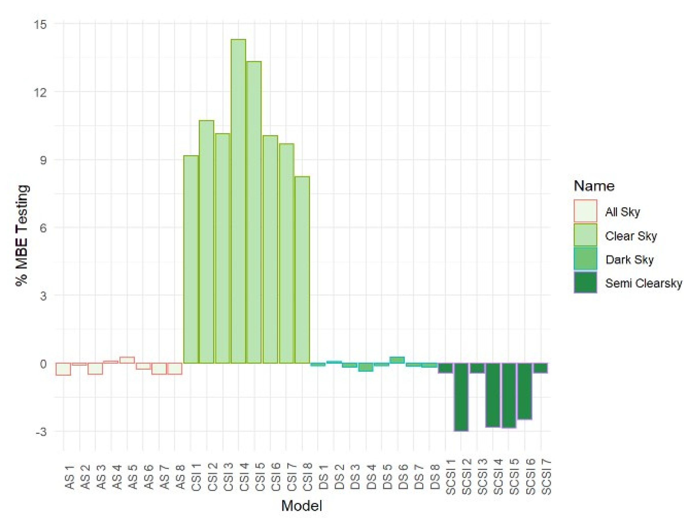
| Model | Equation | R2 Adjust | F Statistic | P Value | RMSE Testing % | MBE Testing % |
|---|---|---|---|---|---|---|
| CSI 1 | 220.535 − 1.415GHI + 41.068α + 27.06ψ − 88.395Kt + 2.048CSG − 12.768Ct − 0.326Sc + 0.289St | 0.889 | 38.88 | 9.21 × 10⁻¹⁴ | 32.45 | 9.16 |
| CSI 2 | 235.119 − 1.251GHI − 114.444α − 158.174Kt + 2.105 CSG | 0.884 | 73.21 | 3.18 × 10⁻¹⁶ | 32.25 | 10.74 |
| CSI 3 | 148.71 − 1.022GHI + 1.727CSG − 13.641Ct | 0.899 | 113.2 | <2.2 × 10⁻¹⁶ | 30.1 | 10.13 |
| CSI 4 | 480.79 + 734.07α − 678.06Kt | 0.881 | 141.2 | <2.2 × 10⁻¹⁶ | 38.65 | 14.3 |
| CSI 5 | 516.66 + 741.42α + 19.24ψ - 767.38Kt | 0.88 | 94.06 | <2.2 × 10⁻¹⁶ | 38.55 | 13.32 |
| CSI 6 | 380.28 + 1661.56α − 159.48α2 − 223.77α3 | 0.896 | 110.7 | <2.2 × 10⁻¹⁶ | 32.12 | 10.06 |
| CSI 7 | 139.243 − 1.469GHI + 28.40ψ + 2.143CSG − 12.825Ct | 0.901 | 87.41 | <2.2 × 10⁻¹⁶ | 31.13 | 9.69 |
| CSI 8 | 68.351 + 0.809CSG − 16.205Ct | 0.894 | 161.2 | <2.2 × 10⁻¹⁶ | 26.8 | 8.25 |
| SCSI 1 | 57.413 + 0.419GHI + 275.76α − 1.298ψ − 20.17Kt + 0.218CSG − 27.118Ct − 0.107Sc − 1.575St | 0.824 | 309.9 | <2.2 × 10⁻¹⁶ | 20.3 | −0.448 |
| SCSI 2 | −104.617 + 0.397GHI + 229.291α + 127.25Kt + 0.294CSG | 0.775 | 455.5 | <2.2 × 10⁻¹⁶ | 23.87 | −3.04 |
| SCSI 3 | 27.481 + 0.346GHI + 0.611CSG − 27.249Ct | 0.823 | 817 | <2.2 × 10⁻¹⁶ | 19.56 | −0.454 |
| SCSI 4 | −295.74 + 682.32α + 516.36Kt | 0.766 | 863.2 | <2.2 × 10⁻¹⁶ | 25.8 | −2.861 |
| SCSI 5 | −297.125 + 678.274α − 2.981ψ + 528.261Kt | 0.765 | 574.9 | <2.2 × 10⁻¹⁶ | 25.78 | −2.868 |
| SCSI 6 | 550.397 + 5584.196α − 655.037α2 | 0.767 | 867.6 | <2.2 × 10⁻¹⁶ | 23.96 | −2.508 |
| SCSI 7 | 23.474 + 0.386GHI + 275.9010α + 0.243CSG − 27.452Ct | 0.825 | 623.4 | <2.2 × 10⁻¹⁶ | 20.33 | −0.448 |
| SCSI 8 | 23.474 + 0.386GHI + 275.9010α + 0.243CSG − 27.452Ct | 0.825 | 623.4 | <2.2 × 10⁻¹⁶ | 20.33 | −0.448 |
| DS 1 | 157.89 + 1.302GHI − 85.187α − 0.839ψ − 369.4Kt + 0.175CSG − 19.147Ct + 0.098Sc − 0.7955St | 0.631 | 504.1 | <2.2 × 10⁻¹⁶ | 37.72 | −0.131 |
| DS 2 | 96.677+1.34.GHI − 75.772α − 332.604Kt + 0.128CSG | 0.604 | 900 | <2.2 × 10⁻¹⁶ | 39.65 | 0.057 |
| DS 3 | 65.088 + 0.939GHI + 0.187CSG − 19.02Ct | 0.627 | 1322 | <2.2 × 10⁻¹⁶ | 37.7 | −0.178 |
| DS 4 | −173.757 + 362.933α + 911.806Kt | 0.548 | 1430 | <2.2 × 10⁻¹⁶ | 41.12 | −0.373 |
| DS 5 | −178.696 + 358.44α − 8.763ψ + 944.08Kt | 0.552 | 967.9 | <2.2 × 10⁻¹⁶ | 40.94 | −0.12 |
| DS 6 | 386.561 + 8448.735GHI − 476.519GHI2 | 0.589 | 1692 | <2.2 × 10⁻¹⁶ | 40.82 | 0.275 |
| DS 7 | 155.66 + 1.31GHI − 87.78α + 2.143Kt − 12.825Ct | 0.631 | 806.7 | <2.2 × 10⁻¹⁶ | 37.76 | −0.149 |
| DS 8 | 199.445 + 1.471GHI − 538.095Kt − 19.135Ct | 0.63 | 1339 | <2.2 × 10⁻¹⁶ | 37.76 | −0.194 |
| AS 1 | 142.8 + 0.991GHI + 43.85α - 2.76ψ − 268.629Kt + 0.121CSG − 23.007Ct + 0.013Sc − 0.276St | 0.697 | 840.3 | <2.2 × 10⁻¹⁶ | 34.45 | −0.527 |
| AS 2 | 81.165 + 1.087GHI + 31.408α − 277.566Kt + 0.087CSG | 0.662 | 1435 | <2.2 × 10⁻¹⁶ | 35.54 | −0.105 |
| AS 3 | 52.665 + 0.715GHI + 0.3CSG − 23.127Ct | 0.692 | 2195 | <2.2 × 10⁻¹⁶ | 34.77 | −0.515 |
| AS 4 | −185.903 + 452.876α + 664.281Kt | 0.586 | 2073 | <2.2 × 10⁻¹⁶ | 39.23 | 0.088 |
| AS 5 | −189.315 + 446.845α − 9.407ψ − 694.068Kt | 0.59 | 1401 | <2.2 × 10⁻¹⁶ | 39.15 | 0.243 |
| AS 6 | 416.734 + 10468.523GHI − 1332.329GHI2 | 0.621 | 2398 | <2.2 × 10⁻¹⁶ | 37.56 | −0.283 |
| AS 7 | 137.629 + 0.986GHI − 2.755ψ − 264.258Kt + 0.18CSG − 23.062Ct | 0.697 | 1345 | <2.2 × 10⁻¹⁶ | 34.46 | −0.511 |
| AS 8 | 168.98 + 1.236GHI − 487.002Kt | 0.659 | 2825 | <2.2 × 10⁻¹⁶ | 35.56 | −0.511 |
Publisher’s Note: MDPI stays neutral with regard to jurisdictional claims in published maps and institutional affiliations. |
© 2022 by the authors. Licensee MDPI, Basel, Switzerland. This article is an open access article distributed under the terms and conditions of the Creative Commons Attribution (CC BY) license (https://creativecommons.org/licenses/by/4.0/).
Share and Cite
Muñoz-Salcedo, M.; Peci-López, F.; Táboas, F. An Empirical Correction Model for Remote Sensing Data of Global Horizontal Irradiance in High-Cloudiness-Index Locations. Remote Sens. 2022, 14, 5496. https://doi.org/10.3390/rs14215496
Muñoz-Salcedo M, Peci-López F, Táboas F. An Empirical Correction Model for Remote Sensing Data of Global Horizontal Irradiance in High-Cloudiness-Index Locations. Remote Sensing. 2022; 14(21):5496. https://doi.org/10.3390/rs14215496
Chicago/Turabian StyleMuñoz-Salcedo, Martín, Fernando Peci-López, and Francisco Táboas. 2022. "An Empirical Correction Model for Remote Sensing Data of Global Horizontal Irradiance in High-Cloudiness-Index Locations" Remote Sensing 14, no. 21: 5496. https://doi.org/10.3390/rs14215496