Article

A Novel Water Index Fusing SAR and Optical Imagery (SOWI)

1
Department of Cartography and Geographical Information Engineering, China University of Mining and Technology, Xuzhou 221116, China
2
International Research Center of Big Data for Sustainable Development Goals, Beijing 100094, China
3
Key Laboratory of Digital Earth Science, Aerospace Information Research Institute, Chinese Academy of Sciences, Beijing 100094, China
4
Satellite Application Center for Ecology and Environment, Ministry of Ecology and Environment of the People’s Republic of China, Beijing 100094, China
5
Institute of Geographical Sciences, Henan Academy of Sciences, Zhengzhou 450052, China
*
Author to whom correspondence should be addressed.
Remote Sens. 2022, 14(21), 5316; https://doi.org/10.3390/rs14215316
Submission received: 7 September 2022 / Revised: 14 October 2022 / Accepted: 19 October 2022 / Published: 24 October 2022

Abstract

:
Continuous and accurate acquisitions of surface water distribution are important for water resources evaluation, especially high-precision flood monitoring. During surface water extraction, optical imagery is strongly affected by clouds, while synthetic aperture radar (SAR) imagery is easily influenced by numerous physical factors; thus, the water extraction method based on single-sensor imagery cannot obtain high-precision water range under multiple scenarios. Here, we integrated the radar backscattering coefficient of ground objects into the Normalized Difference Water Index to construct a novel SAR and Optical Imagery Water Index (SOWI), and the water ranges of five study areas were extracted. We compared two previous automatic extraction methods based on single-sensor imagery and evaluated the accuracy of the extraction results. Compared with using optical and SAR imagery alone, the accuracy of all five regions was improved by up to 1–18%. The fusion-derived products resulted in user accuracies ranging 95–99% and Kappa coefficients varying by 85–97%. SOWI was then applied to monitor the 2021 heavy rainfall-induced Henan Province flood disaster, obtaining a time-series change diagram of flood inundation range. Our results verify SOWI’s continuous high-precision monitoring capability to accurately identify waterbodies beneath clouds and algal blooms. By reducing random noise, the defects of SAR are improved and the roughness of water boundaries is overcome. SOWI is suitable for high-precision water extraction in myriad scenarios, and has great potential for use in flood disaster monitoring and water resources statistics.

Graphical Abstract

1. Introduction

Water is the basic resource of human production and life [1]. It is, therefore, critical to quickly and accurately obtain data on the distribution of surface waterbodies in the fields of natural disaster monitoring and assessment, ecological environment protection, and macro-control of water resources [2,3]. With the successful launch of the European Sentinel series [4,5], the United States’ Landsat series [6,7], and China’s Gaofen (GF) series satellites [8,9], remote sensing data of multi-temporal scales and types within the same area can be obtained [10]. Various types of remote sensing data can be utilized to comprehensively and effectively monitor the distribution of surface waterbodies [11]. In the past few decades, researchers have proposed a variety of optical or synthetic aperture radar (SAR) imagery-based methods to extract the water distribution [12,13,14,15].
To obtain the surface water distribution from optical remote sensing imagery, object-based approaches and pixel-based thresholding methods can be used [16,17]. In the object-based approach, mainly the spectral, shape, structure, and textural features of ground objects are used to extract waterbody information [18]. The pixel-based threshold approach is mainly based on the spectral characteristics of ground objects and spectral information, which is utilized to construct various classification models and waterbody indices to extract waterbodies [19]. Among the pixel-based threshold methods, the spectral water index method has the advantages of high computational efficiency, low computational cost, simplicity, and wide generalization; thus, it is currently the most widely used technique [20]. Water indices based on optical images mainly include the Normalized Difference Water Index (NDWI) [21], Modified Normalized Difference Water Index (MNDWI) [22], Automated Water Extraction Index (AWEI) [15], and Superfine Water Index (SWI) [14]. Because the water index is constructed by using the spectral characteristics of the waterbody within optical imagery [23], the accuracy of the waterbody recognition based on the water index can be significantly affected if weather and/or light conditions interfere with the optical image [24]. In addition, optical imagery cannot penetrate vegetation; thus, it is difficult to detect waterbodies covered by vegetation [25].
SAR data are obtained with active sensors at longer wavelengths, which can penetrate clouds and vegetation to varying degrees; thus, ground object information can be obtained throughout the day [26]. The waterbody has a high dielectric constant, while its surface is smooth; thus, because the backscattering method is mainly specular scattering, the backscattering coefficient of the waterbody in SAR imagery is small [27]. Therefore, researchers have proposed many SAR image waterbody segmentation methods [28]. The use of SAR imagery to obtain the distribution of waterbodies has advantages. For example, the distribution of surface waterbodies can be monitored under all weather conditions. However, the side-view imaging of SAR imagery leads to radar shadows in areas with large terrain fluctuations, which affect the accuracy of waterbody extraction [29]. Windy weather tends to generate waves on the surface of the waterbody, increasing the backscattering coefficient of the waterbody, and causes the omission of waterbody extraction [30,31]. Moreover, the planktonic algae represented by algal blooms can release biosurfactants which reduce the backscattering of radar waves [32], and the backscattering ability is close to that of water, so it will not interfere with the water extraction process. However, the surface roughness of emergent vegetation such as water hyacinth is relatively large; thus, it can produce a high amount of volume scattering, resulting in missing the extraction of water underneath such vegetation.
While SAR images tend to have lower spatial resolution and more noise, they can provide valuable information in cloud-covered and shadowed areas. In contrast, optical images have higher spatial resolution and rich spectral information, but are greatly affected by clouds and vegetation in waterbody identification. Therefore, when using only one type of data (either optical or SAR) to extract a surface waterbody, it is difficult to obtain a continuous and complete distribution if the area is covered by clouds for an extended period of time or if the terrain greatly fluctuates [33]. Considering the advantages and disadvantages of both optical and SAR imagery, researchers have proposed multiple methods to extract surface waterbodies by combining the two image types. Hong et al. [34] used optical data to generate land cover maps and determine the thresholds of SAR and digital elevation model (DEM) data for water extraction, which improved the water extraction accuracy. Irwin et al. [2] adopted a multi-level decision tree model to achieve the high-precision extraction of waterbodies from SAR imagery, optical satellite-based imagery, and airborne light detection and ranging (LiDAR). Shahryar et al. [27] fused optical (Landsat-8, Sentinel-2) and SAR (Sentinel-1) data to obtain the distribution of waterbodies in South Asia using a decision tree model. A series of water extraction models that integrate SAR and optical imagery has also been established, but most were constructed using multi-level decision tree models based on three or more data types [2,4,11,27,34,35]. A complex decision tree model is required and three types of remote sensing data must be obtained for the same area at similar times, making it difficult to simply or quickly obtain the distribution of surface waterbodies.
In order to fully combine the complementary advantages of SAR and optical imagery, fast water extraction can be realized in complex scenes, so as to provide a correct water distribution range for water resources statistics, flood disaster monitoring, and water environment protection. This study attempts to establish an all-weather, automated water extraction method with high accuracy. To achieve this, first, the optical and SAR imagery of the study area were obtained, and the NDWI based on optical imagery was modified by the SAR imagery ground object backscattering coefficient to obtain the SOWI. Then, the threshold method was used to obtain the water range. Finally, the results were compared with the water extraction method based on a single remote sensing image, and SOWI was applied to flood disaster monitoring in Xunxian County, Henan Province to verify its applicability.

2. Study Area and Data
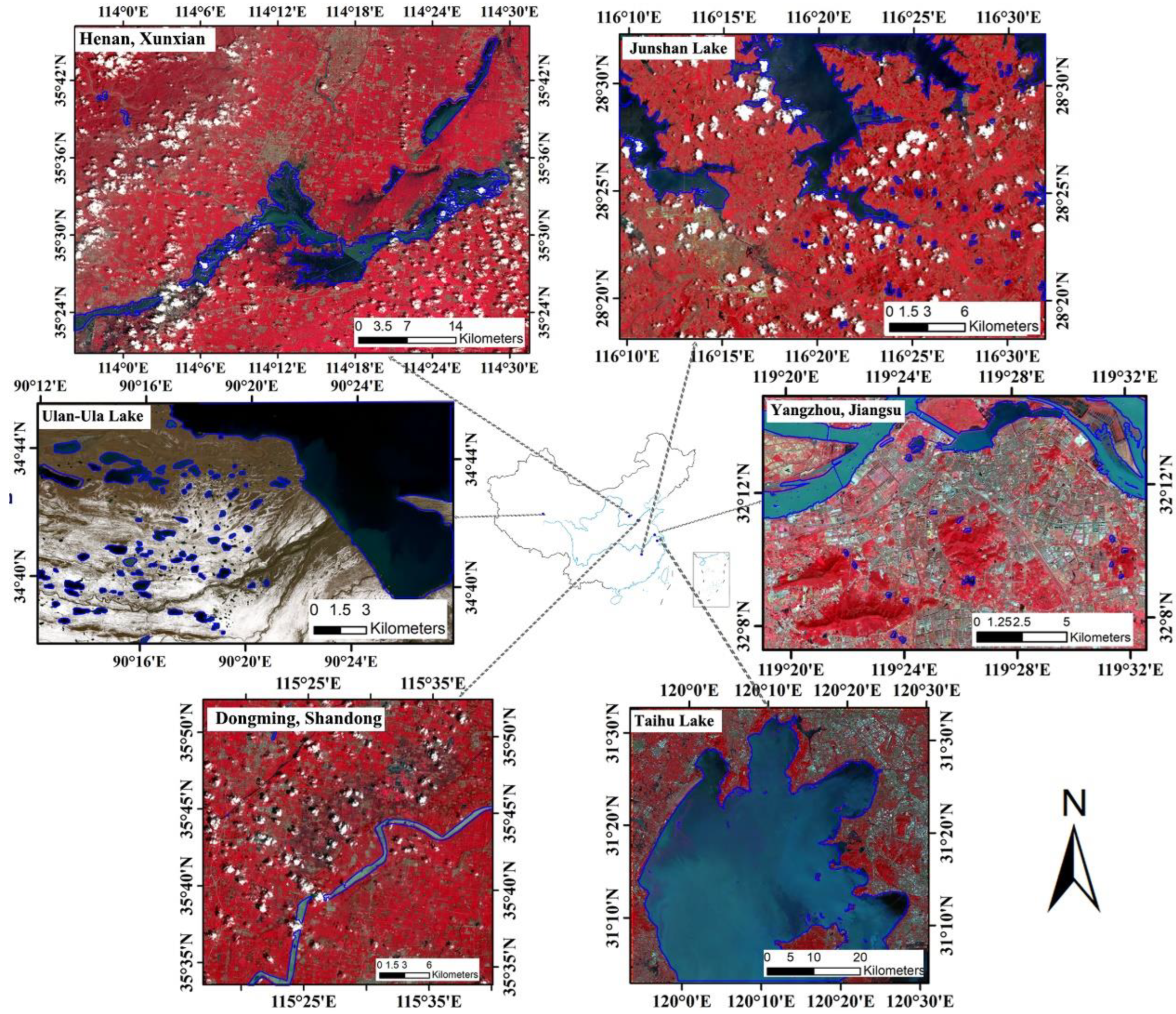
2.1. Study Area

Multiple waterbody types were selected under different climatic and different geographical conditions to test the accuracy and robustness of SOWI. These include: Xunxian County in Henan Province, the Dongming Section of the Yellow River in Shandong Province, Junshan Lake, Taihu Lake, Yangzhou in Jiangsu Province, and Ulan-Ula Lake in Xinjiang, covering the eastern, central, and western regions of China (Figure 1). The overall study area includes rivers, large lakes, and urban waterbodies. Different types of waterbodies differ in terms of depth, transparency, shape, and vegetation coverage. The weather conditions during the image data collection period included windy, cloudy, and cloudless (Table 1). From the combination of the overall study area and the weather conditions at the time of image acquisition, the sub-scene contains complex surface features. The terrain of Xunxian County, Henan Province fluctuates greatly, and there was a high amount of cloud cover during the image collection period. Wulan Wula Lake, which is semi-annular, is the largest lake in the Hoh Xil region. The lake topography consists of mostly gentle slopes and hilly areas, while the surrounding landscape is mainly Gobi Desert, and the water quality is relatively pure, with no phytoplankton cover. The surface elevation of the lake is 4854 m, and the surface area of the lake is 612 km2. Due to the strong wind speed in that area, a large number of waves were generated on the lake surface. Taihu Lake is the second largest freshwater lake in China, with an area of 2338 km2. In recent years, the eutrophication problem in Taihu Lake has become increasingly serious, and the explosive growth of algae has accelerated the deterioration of the water environment. During the image collection period in the Taihu Lake area, an algal bloom erupted. Junshan Lake is 25 km in length from north to south, typically about 5 km wide from east to west, and 16 km wide at its widest part, with a surface area of 320,000 km2 and a drainage area of 616 km2. The main aquatic plants in Junshan Lake include black algae, bitter grass, wild water chestnut, lotus, Maleophil, and others. The phytoplankton mainly include microcystis, Streptomyces, chattering algae, anabaena, and others. There was cloud occlusion in the optical image of the surrounding Junshan Lake area, which also contains many smaller waterbodies. The study area in Yangzhou, Jiangsu mainly features a large number of urban buildings.

2.2. Satellite Data Collection and Preprocessing

In the study area, Sentinel-2/Multispectral Imagery (MSI) data and GF6/Wide Field of View (WFV) imagery data were used for optical images and Sentinel-1 Single Look Complex (SLC) and GF-3 FSII data were used for SAR images.
(1) Sentinel-1 SLC data: Interferometric Wide Swath (IW) and Sentinel-1 data have a wide-ranging resolution of 5 m, azimuth resolution of 20 m, and revisit period of 6 days. The data are mainly processed by the SNAP 9.0.0(SeNtinel Applications Platform) software. Multi-polar SAR data are corrected by using the precise orbit file. Subsequently, the thermal noise in the image is removed and the backscattering coefficient of the ground object is obtained by radiometric calibration. Multi-look processing is then performed and the speckle noise in the image is weakened with a refined Lee filter [35]. Finally, DEM data are used for the geometric correction of the image to eliminate the geometric distortion of the image [36]. In general, co-polarization (VV, HH) is more effective for surface scatterers, such as waterbodies, while cross-polarization (VH, HV) is more effective for volume scatterers, such as forests [37]. Previous results proved that co-polarization is more suitable for surface water detection than cross-polarization [38]. The VV polarization of Sentinel-1 data was selected for the SAR data of the study area.
(2) Sentinel-2 MSI data: For this type of data, the total radiance value of the ground objects collected by the sensor is not the real reflectivity of the ground surface. It needs to be processed by atmospheric correction to obtain the real reflectivity of the ground target [39,40]; thus, the images processed in this study were Level 2-A. Pre-processed Sentinel-2 L2A data can be directly downloaded from the official European Space Agency website.
(3) GF-3 FS II data: GF-3 has a variety of image modes. In this study, FS II data with a standard spatial resolution of 10 m were used. First, the data were multi-look-processed and refined Lee filtering was used to eliminate speckle noise. Subsequently, DEM data were used for the geometric correction. The HH polarization of GF-3 data was selected for the SAR data of the study area.
(4) GF6-WFV data. The multispectral medium-resolution wide-format camera carried by GF-6 has a standard spatial resolution of 16 m and observation width of 800 km. The GF-6 WFV L1A level data must be processed by orthophoto, radiation, and atmospheric corrections.

3. Methods

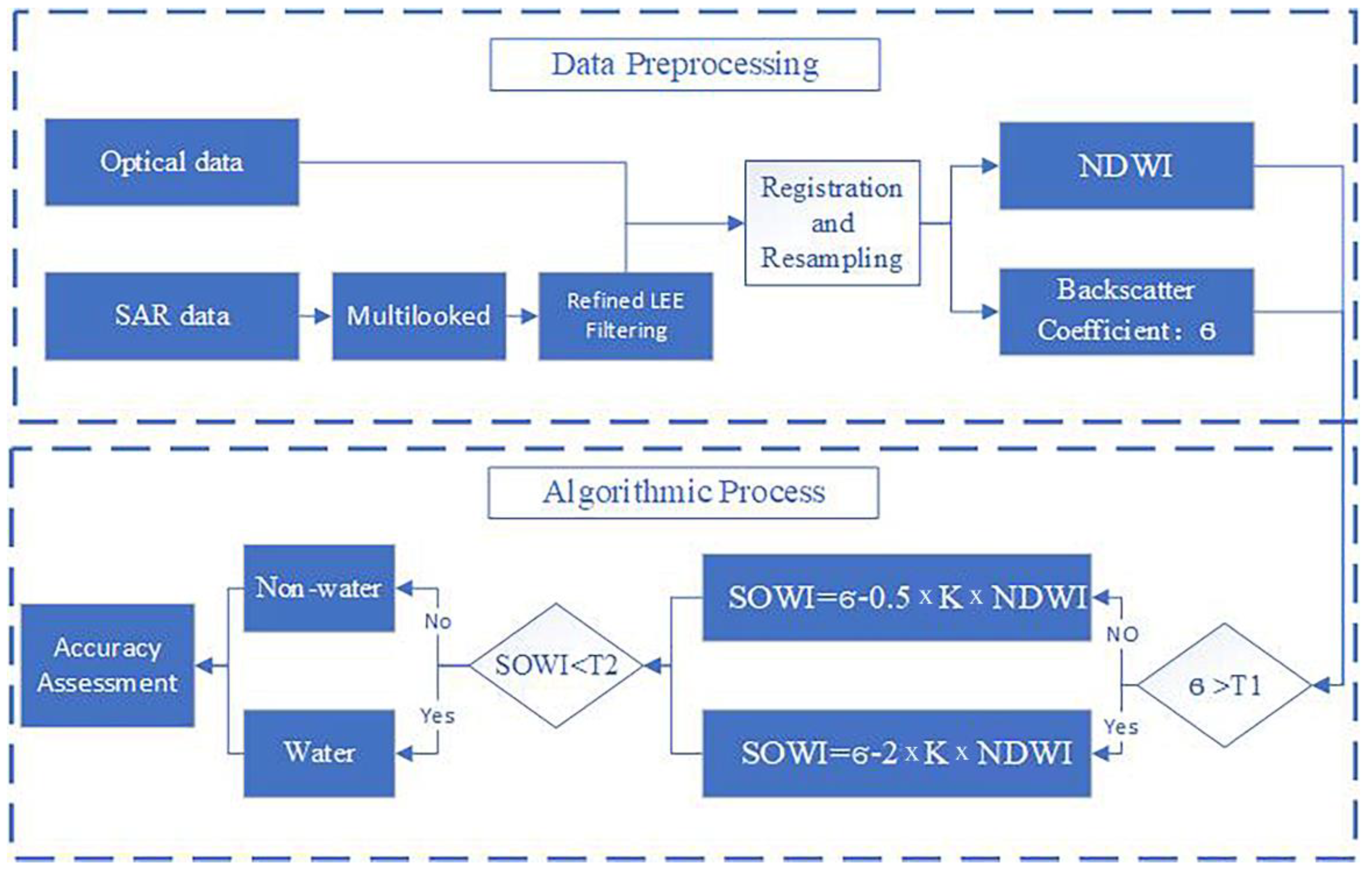
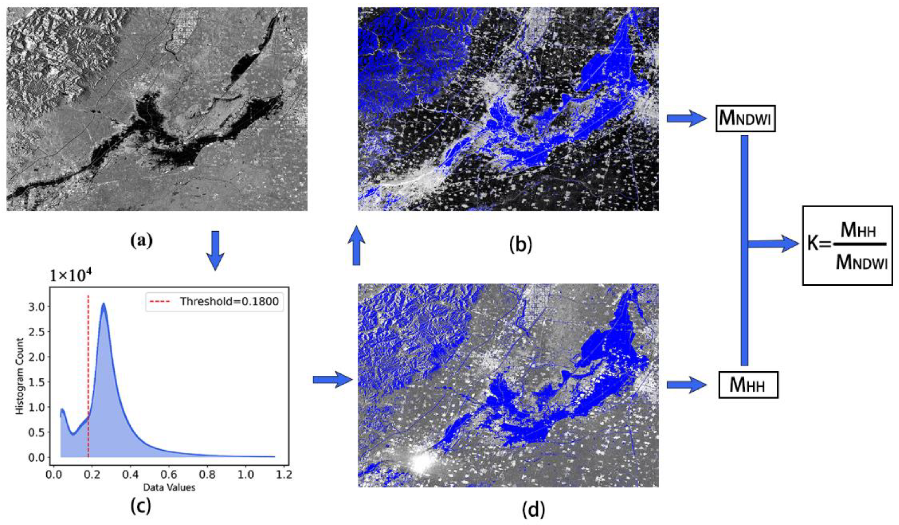
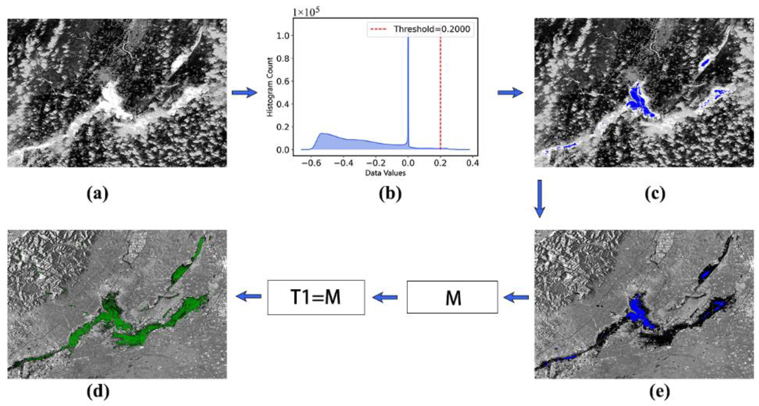
3.1. Technical Framework

The framework in which SOWI was used to obtain the distribution of surface waterbodies in this study is shown in Figure 2 and can be described as follows. First, the preprocessed SAR and optical images are registered and then resampled to the same resolution. Based on certain rules, a threshold T1 is determined for each SAR image, the SAR image is preliminarily segmented according to T1, different coefficients K are assigned to the preliminary segmentation results, and the SOWI value is calculated. The threshold value method is used to determine the threshold of the operation result to obtain the distribution of the surface waterbody and the accuracy of the result is evaluated.

3.2. SOWI Model Building

The absorption of 0.4 to 2.5-μm electromagnetic waves by waterbodies is significantly higher than that of most ground objects, so the reflectivity of waterbodies in multispectral remote sensing images tends to be low. In the visible light range, the reflection of water is mainly concentrated in the blue-green band and gradually decreases with the increase of wavelength. In the near-infrared and mid-infrared bands, the waterbody absorbs almost all the incident energy, while vegetation, soil, and other ground objects have higher reflectivity, which makes the pure waterbody distinct from the vegetation and soil in these two bands. The waterbody index method is based on the analysis of the spectral characteristics of the waterbody; it selects the bands closely related to the waterbody identification, analyzes the relationship between the waterbody and the spectral value by building a waterbody index model, and gives the corresponding threshold value to realize the extraction of waterbody information.
NDWI (Equation (1)), as a classic waterbody index model, uses the spectral characteristics of the waterbody to select the green light and near-infrared bands for band calculation. The index can effectively distinguish the waterbody from vegetation and the shadow of mountains [20,41]. When the NDWI of an area is greater than the appropriate threshold ( T N D W I ) , this area is identified as waterbody as follows:
NDWI = (Green − NIR)/(Green + NIR).
The magnitude of the backscattering intensity of SAR images is closely related to the surface roughness of the ground objects; furthermore, the smooth surface of the waterbody is dominated by specular scattering. Compared with the land dominated by volume scattering, the backscattering ability of the waterbody to the radar signal is weaker. The waterbody with an approximately smooth surface has a low gray value in the SAR image, which is characterized by a dark area. The waterbody segmentation threshold is usually obtained by solving the extreme points of the grayscale histogram of the image, and the part of the image that is smaller than the threshold value is marked as a waterbody [27]. When the backscattering coefficient of the ground objects ( σ ) in the SAR image is smaller than the appropriate threshold ( T σ ), this area is considered to be a waterbody.
To sum up, the equations for the identification of ground objects as waterbodies from optical and SAR images are as follows.
SAR data:
σ   < T σ .
Optical data:
NDWI   >   T N D W I .
Equations (2) and (3) are used to obtain the equation for jointly identifying ground objects as waterbodies in optical and SAR images:
σ NDWI   <   T σ   T N D W I
Because T σ and T N D W I are both constants, T σ T N D W I can be simplified as constant T, and thus, Equation (4) can be simplified as follows:
σ NDWI   <   T .
The NDWI and σ significantly differ. When σ is used to directly subtract the NDWI, σ —NDWI is approximately equal to the NDWI because the latter is much larger than σ , which mainly reflects the optical properties of ground objects. To accurately reflect the spectral and backscattering characteristics of ground objects when σ is subtracted from NDWI, it is necessary to multiply the NDWI by the coefficient K to compensate for the data difference between the NDWI and σ . The equation for the identification of ground objects as waterbodies based on the combination of SAR and optical images is as follows:
σ K × NDWI < T .
The initial SOWI equation is as follows:
SOWI = σ K × NDWI .
The purpose of this study is to combine the advantages of SAR image and optical image to realize high-precision automatic water extraction in various scenes, such as cloud, radar shadow, and wind waves. SAR image can obtain the water area under clouds, so as to overcome the defects of optical image. However, SAR image are difficult to obtain the accurate water extraction from the area with small backscattering coefficient, which usually include radar shadows, uneven water surfaces, and smooth ground objects [42,43]. When extracting water from the above ground objects, it is necessary to make a comprehensive judgment based on the spectral characteristics of the ground objects. Therefore, the main area for comprehensive analysis combined with optical images and SAR images is the area with a small backscattering coefficient of the ground objects. The process should therefore be to calculate the average value of backscatter coefficient and NDWI in this area ( M N D W I , M H H ), and divide the two to obtain the coefficient K value. The coefficient K can balance the difference between the NDWI value and the backscattering coefficient value in this area, and the water distribution range can then be obtained by comprehensively analyzing the spectral characteristics and backscattering characteristics of ground objects. Figure 3 shows that the area with small backscattering coefficients in the SAR image is obtained (blue area in Figure 3) based on the frequency distribution histogram of the SAR image. By calculating the mean values of the NDWI and backscatter coefficients in the blue area and dividing the two, the coefficient K of the SOWI algorithm of the image is obtained.
Since optical images and SAR images have different advantages, the coefficient K should be scaled for different situations. This process can be described as follows. Firstly, the initial threshold value T1 for water extraction is set for the SAR image. The area with the backscattering coefficient less than T1 in the SAR image is the area that can be accurately judged as the waterbody according to the backscattering coefficient of the ground objects. At this time, the coefficient K of the NDWI is reduced to weaken the influence of the optical image on the judgment of ground objects in this area. If the area contains clouds or vegetation, then the identification of ground objects is mainly based on the SAR image information due to the small proportion of optical images, and in this way, the distribution of waterbodies in this area can be determined. In the area where the backscattering coefficient of the ground object is greater than T1, it is difficult to obtain the correct water distribution from the SAR image. That area often includes radar shadows, uneven water surfaces affected by strong winds, smooth bare soil, and other ground objects with similar backscattering coefficients. Therefore, it is necessary to increase the coefficient K in that area to enhance the effects of optical images on the identification of ground objects and use the spectral characteristics of ground objects for the evaluation.
It is difficult to determine the threshold T1 only from SAR images, so this study uses optical images to assist SAR images to determine the threshold T1. First, use the waterbody index to obtain the accurate waterbody area. Refer to the dynamic range of the NDWI threshold for waterbody extraction found by Zhang, i.e., −0.184 to 0.228 [44], and the larger the NDWI value, the greater the possibility that the pixel is a waterbody. Therefore, take 0.228 and reserve one decimal place as the threshold value, and the pixel value greater than 0.2 is classified as a waterbody pixel. Then, since this area is only determined by the waterbody index, it is randomly distributed in the water area of the SAR image. Finally, the average value of backscattering coefficients in the above regions is counted as the final threshold T1. As shown in Figure 4, when 0.2 is chosen as the threshold, an accurate waterbody range can be obtained even if there is a large amount of cloud occlusion in the image; furthermore, there is no situation in which non-waterbody pixels can be identified as waterbody. These pixels determined as water are relatively uniformly distributed in the water area (blue area in Figure 4) of the SAR image. The average backscattering coefficient of the points where the pixels are located is counted as the threshold T1, and the water area (green area in Figure 4) of the SAR image can be correctly extracted, with few commission errors.
The SOWI calculation equation of the subregion can be obtained as follows. When areas are preliminarily identified as waterbodies from SAR images ( σ < T1), the calculation is:
SOWI = σ 0.5 × K × NDWI ,
When areas are preliminarily identified as non-waterbodies from SAR images ( σ > T1), the calculation is:
SOWI = σ 2 × K × NDWI .
The scaling factor before the K value is an empirical result determined from the reflectivity patterns observed on pure pixel datasets of different land cover types. The iterative method is used to obtain parameters for the purpose of maximizing the separability of reflectivity between water and non-water objects. In the final indexing process, for the convenience of use, after rounding the coefficients, it is finally determined that the optimal result can be obtained when K is scaled by a factor of 2.

3.3. Extraction of Water Based on Visual Interpretation

Manual visual interpretation (also known as visual interpretation), a type of remote sensing image interpretation, is the inverse process of remote sensing imaging. It refers to the process of obtaining specific target ground object information on remote sensing images by professionals either through direct observation or assisted by interpretation instruments. Manual visual interpretation refers to the extraction of useful information from remote sensing images through brain analysis, reasoning, and judgment by relying on human eyes and the knowledge, experience, and relevant information mastered by the interpreter, and this technique is characterized by high accuracy [10].
Waterbodies in remote sensing images have distinct features in terms of color, brightness, texture, and shape. For example, clear or deep water is blue-green, and the water color changes from blue to green and yellow with the increase of turbidity. When the sediment content in the water is close to saturation, the water color is also close to the color spectrum of the sediment itself. Compared with other ground objects, the overall reflectance of water body is low, mainly concentrated in the visible band. Above 0.7 μm, due to the serious absorption of infrared light by water, the reflectance of water is very low. Owing to the low reflectance of water, sometimes, the brightness of its image is relatively low, which is close to the brightness of the shadow in the image. With an increase of suspended sediment concentration (i.e., turbidity) in the water, the volume reflection brightness of the waterbody in the whole visible spectral segment increases, especially in the yellow and red light areas [16], and the water image becomes increasingly brighter compared to the dark areas. The surface of calm water is very smooth, and thus, its internal texture and structure are clearly different from that of land and vegetation. Moreover, the shape of the waterbody formed in a natural state has obvious irregularity. Rivers often have branches and form tree-like structures, while the boundaries of lakes are highly irregular and random. These characteristics give waterbodies a strong identification function compared to many other types of ground object in nature. Therefore, the water area as interpreted by manual visual interpretation is usually regarded as the true value, and thus, it is usually used as a basis for the accuracy evaluation of later experimental results [15,45,46].
In this study, the surface water distribution was obtained by manual visual interpretation as the basis for accuracy evaluation. First, Sentinel-2 images and artificial visual interpretation were used to obtain real water distribution data in the study area. Then, to determine the area of the waterbody under cloud occlusion in the Sentinel-2 image, Sentinel-1 and -2 images without cloud occlusion in a similar period were used. Next, Sentinel-1 and Google Earth images of the same period were then used to identify ground objects that were difficult to recognize in the Sentinel-2 images. Finally, the water distribution range of five study areas was obtained.

3.4. Accuracy Evaluation

The overall accuracy, producer accuracy, user accuracy, and Kappa coefficient were obtained from the distribution range of surface waterbodies obtained by various algorithms and the distribution range of real waterbodies, which were used to evaluate the accuracy of the algorithm waterbody extraction results. The producer accuracy characterizes the probability of missing classification results, while the user accuracy represents the probability of misclassification in the classification results, and the overall precision represents the percentage of correctly classified areas in the total area. Finally, the Kappa coefficient represents the difference between the classification results and random classification. The equations are as follows:
OA = T P + T N T P + F P + F N + T N
UA = T P T P + F P  
PA = T P T P + F N
Kappa = P 0 P e 1 P e
where OA, UA, PA, and Kappa represent the overall accuracy, user accuracy, producer accuracy, and Kappa coefficient, respectively; TP is the number of pixels that are correctly predicted as positive examples; TN represents the number of pixels that are correctly predicted to be negative examples; FP represents the number of pixels that are incorrectly predicted to be positive examples; FN is the number of pixels that are incorrectly predicted to be negative examples; P 0 is the overall classification accuracy; and P e is the product of the total number of real reference pixels in each category and the total number of classified pixels in that category.

4. Results and Analysis

4.1. Overview

In this study, the NDWI and SOWI were calculated from Sentinel-1 and -2 images of Yangzhou, the Shandong Dongming Section of Yellow River, Taihu Lake, Ulan-Ula Lake, and Junshan Lake obtained at similar times. The bimodal threshold method was used to obtain the water distribution from the NDWI, VV polarization, and SOWI and the result of the manual visual interpretation was used as the true value for the accuracy evaluation and analysis. Note that optical images cannot obtain the spectral features of ground objects under cloud occlusion, and the water extraction algorithm based on optical images cannot solve this problem for the time being. Therefore, this study only uses NDWI for comparison. In order to test the application potential of the algorithm, this study selected Sentinel-1, Sentinel-2, and GF-3 images during the heavy rainfall on 20 July 2021 in Henan province to continuously monitor the changes of flood inundation area by the SOWI algorithm.

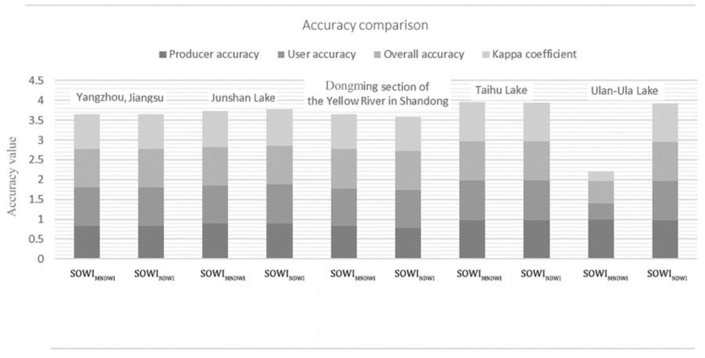
4.2. Precision Analysis and Evaluation
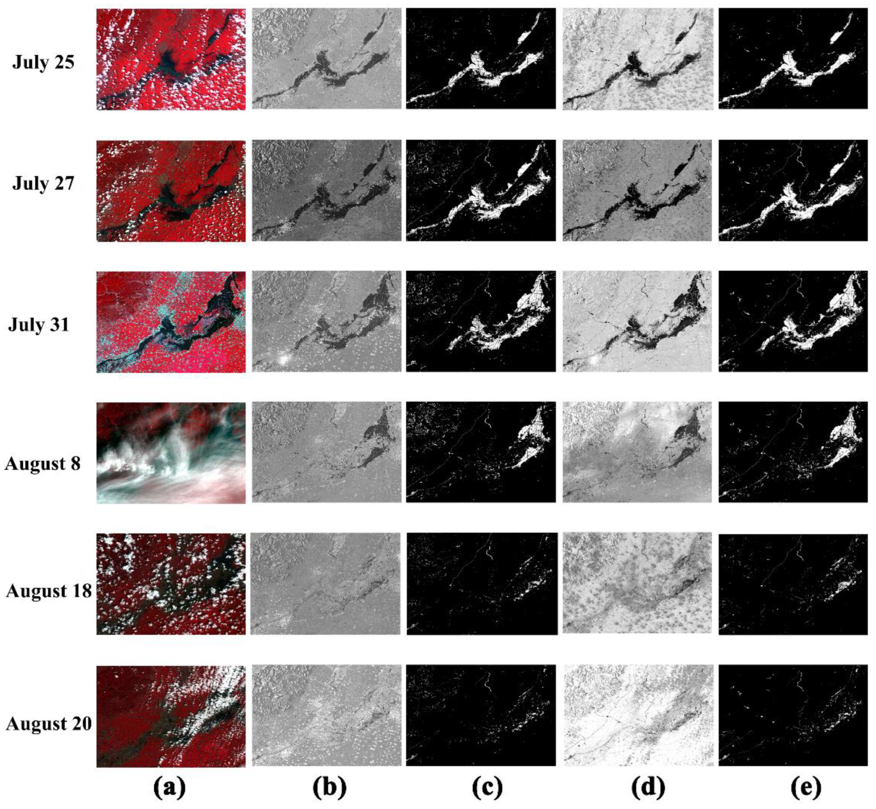
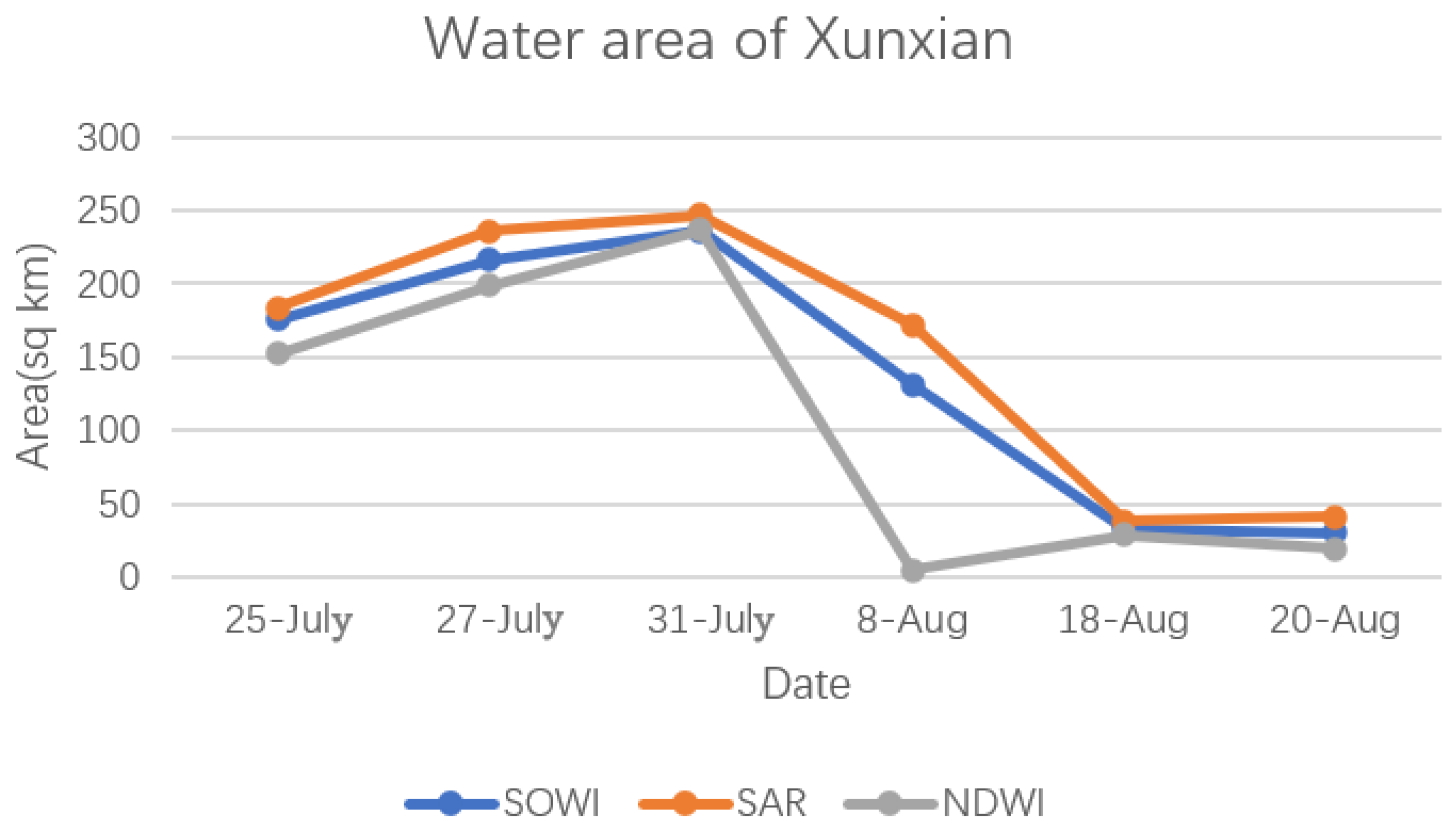
The accuracy evaluation results of the five study areas are shown in Table 2. Overall, the extraction results of the SOWI algorithm combining optical images and SAR images are better than those based on optical images or radar images. Compared with NDWI, the extraction results of SOWI algorithm in Taihu Lake covered by the bloom showed that the producer accuracy increased by 9%, the overall accuracy increased by 6%, and the Kappa coefficient increased by 14%. The SOWI algorithm better obtained the waterbody scope covered by the algal bloom. Using only SAR imagery, the interference of urban buildings and mountains around the Taihu Lake area will cause the image to identify that area as a waterbody. Therefore, compared with the waterbody extraction results of SAR images, the user accuracy of the SOWI algorithm increased by 3%, the overall accuracy increased by 1%, and the Kappa coefficient increased by 4%. In the Ula-Ula Lake area where strong winds frequently occur, the surface of the ground objects is relatively smooth. Therefore, a large number of waterbodies were misclassified as land. Using only SAR imagery, the producer accuracy of waterbody extraction was only 7%, the overall accuracy was 70%, and the Kappa coefficient was 9%. In contrast, as the SOWI algorithm incorporates optical images, its producer accuracy was increased to 97%, the overall accuracy was increased to 98%, and the Kappa coefficient was increased to 97%.
When the SAR image or optical image suffers less interference, the extraction accuracy is not better than that obtained by using the SOWI algorithm. For example, there was no interference from algal blooms and clouds in Yangzhou, Jiangsu. Compared with optical images, the extraction by the SOWI algorithm improved the producer accuracy by 3%, while the user accuracy was the same, the overall accuracy was increased by 1%, and the Kappa coefficient increased by 2%. The extraction error of the optical image in that area is mainly due to the misidentification of the shallow water area of the river channel as land, while the SAR image performed well in the shallow water area. However, the speckle noise in the SAR image was difficult to eliminate. Compared with the SOWI algorithm, the producer accuracy was reduced by 9%, and the extraction of small waterbodies was omitted.
Overall, the experimental surface water area in this study covers the eastern, central, and western regions of China and includes rivers, lakes, urban waterbodies, and small inland waters in northwestern China. The interferences due to clouds, wind, and other weather conditions were also considered. The SOWI yielded a complete water extraction, reflecting the wide applicability of the SOWI algorithm.

4.3. Case Study

In July 2021, the Henan Province, especially the Xunxian County of Hebi City, received extremely heavy rainfall. After 20 July, the water levels of the Communist Canal and Wei River near Xunxian County increased and water seepage and overflow occurred in many embankments. Eventually, several embankments burst, causing widespread damage.
In this study, GF-3, GF-6, Sentinel-1, and Sentinel-2 remote sensing data obtained during the torrential rain period from July to August 2021 in Xunxian County, Henan Province were used with the SOWI algorithm and SAR image thresholding algorithm to create time series diagrams of flood changes from July to August (Figure 5). The figure shows that the flood submerged large tracts of farmland and villages due to the embankment of the Wei River in Xunxian County on 23 July 2021. Therefore, the flood area along the Wei River notably increased, as is confirmed in the data from 25 and 27 July. On 29 July, flood discharge started in Wangzhuang Town, Xunxian County. The waterbody extraction results obtained on July 31 show that the flood area in Xunxian County had reached the maximum. Due to the flood discharge from the downstream, the width of the upstream river significantly decreased. Since August, large-scale heavy rainfall has not occurred in Xunxian County and its upstream area. Based on the water extraction results obtained on 8 August, the flood gradually receded along the Wei River, although the amount of water in the flood discharge area of Xunxian County remained large. The image taken on August 18 shows that the area of the waterbody in the flood discharge area further decreased. By 22 August, the flood in Xunxian County had receded.

4.3.1. Accuracy Evaluation of the Long Time Series Frequency Map Level

The flood area obtained by the three algorithms in each period was calculated in order to verify the effectiveness each algorithm for flood distribution monitoring. As can be seen from Figure 6, the areas extracted by the SOWI and SAR image threshold algorithms held the same trend over time, while that extracted by the NDWI algorithm based on optical imagery indicates that the water area changed greatly around 8 August. Most of the water areas in the optical image of 8 August were covered by clouds, resulting in a much lower flood area extracted by the optical image than by the other two algorithms. The water area extracted by the SAR image was higher than that extracted by the SOWI algorithm in each period. This is because the northwest terrain of this region is mainly mountainous and has great relief, which is represented as radar shadow in the SAR image, and so that region was mistakenly categorized as waterbody (Figure 5). However, the optical image is disturbed by clouds and fog, and thus, the water area was relatively small. It can also be seen from the figure that on 31 July, the difference between the water area extracted by the NDWI and SOWI algorithms is small. There is no cloud occlusion in the optical image on 31 July, and the water extraction accuracy was high, which is consistent with the water area extracted by the SOWI algorithm. By comparing the results of the different algorithms, it can be seen that the spatial and temporal distribution of the flood range extracted by the SOWI algorithm is consistent with the actual changes. The algorithm successfully used optical images to correctly identify radar shadows and reduce commission error, and utilized the SAR images to correctly obtain the range of water under the cloud and fog occlusion, thereby reducing omission error. This demonstrates that the SOWI algorithm is suitable for monitoring the distribution of flood waters during a flood outbreak.

4.3.2. Accuracy Evaluation on the Pixel Level

It is difficult to obtain ground measured data during a flood outbreak period. Meanwhile, due to the influence of cloud occlusion in the optical image during the flood image outbreak period, it is also difficult to use the manual visual interpretation method to comprehensively judge the water distribution range of the whole image by SAR image and optical image. Therefore, this study randomly generated 200 feature points in the image, and then used manual visual interpretation to determine whether the feature points were water pixels. If it was too difficult to accurately determine whether the feature points were water pixels through SAR images and optical images, a different feature point was randomly selected. At the same time, in order to evaluate the accuracy of SOWI in different scenarios, 200 feature points were selected from images on 31 July (without cloud occlusion) and 8 August (with a large amount of cloud occlusion).
According to the accuracy evaluation index based on feature points (Table 3), the cloud and fog coverage in the image on 31 July was less, and the accuracy evaluation index of NDWI and SOWI was close to and above 80%, indicating a high accuracy. The SAR image misclassified the radar shadow in the northwestern mountainous area as water, resulting in a user accuracy of only 75.9%. In the optical images on 8 August, for which there was a large amount of cloud occlusion, the accuracy of the generator of NDWI extraction results was only 14.5%, and a large number of waterbodies under cloud occlusion were omitted from extraction. In the northwest mountainous area with low cloud coverage, SOWI reduced the error of radar shadow extraction with the help of optical images. Compared with SAR images, its user accuracy was improved by 9.7%.

5. Discussion

The new water extraction index proposed in this study improves the accuracy of surface water mapping and change analysis for various environmental studies and applications. SOWI has the characteristics of simplicity and convenience, and shows strong robustness in various environmental conditions and different types of waterbodies.

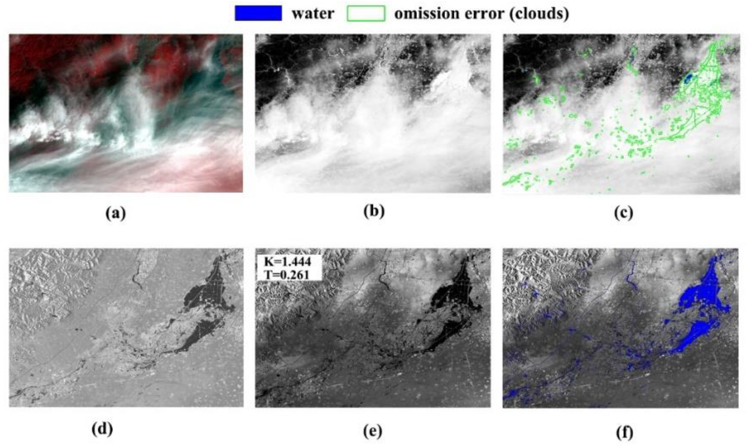
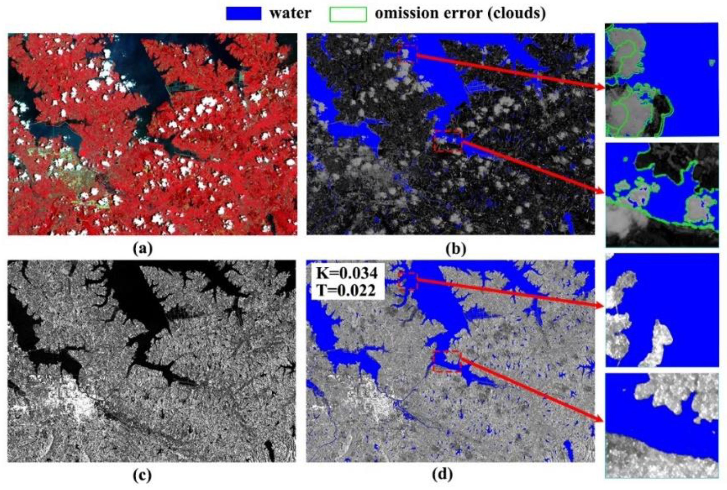
5.1. Waterbodies Covered by Clouds

Although optical images can be used for accurate extraction of waterbodies, the presence of clouds in the images can severely limit the field of application. For example, in the optical images of the Junshan Lake and Xunxian areas of Henan, there are different degrees of cloud coverage. In the optical image extraction results shown in Figure 7, a large number of omissions and extraction errors occurred in the waterbody range obtained by NDWI, which seriously limited its application in terms of water resource change monitoring and flood disaster monitoring. With the help of the ability of SAR images to penetrate through clouds and fog, the SWOI algorithm can obtain relatively accurate extraction results under different cloud conditions (Figure 7 and Figure 8), which verifies its strong robustness. The SOWI algorithm performs well in the cloud cover area, filling the gap caused by high cloud cover in the long-term monitoring of optical images.

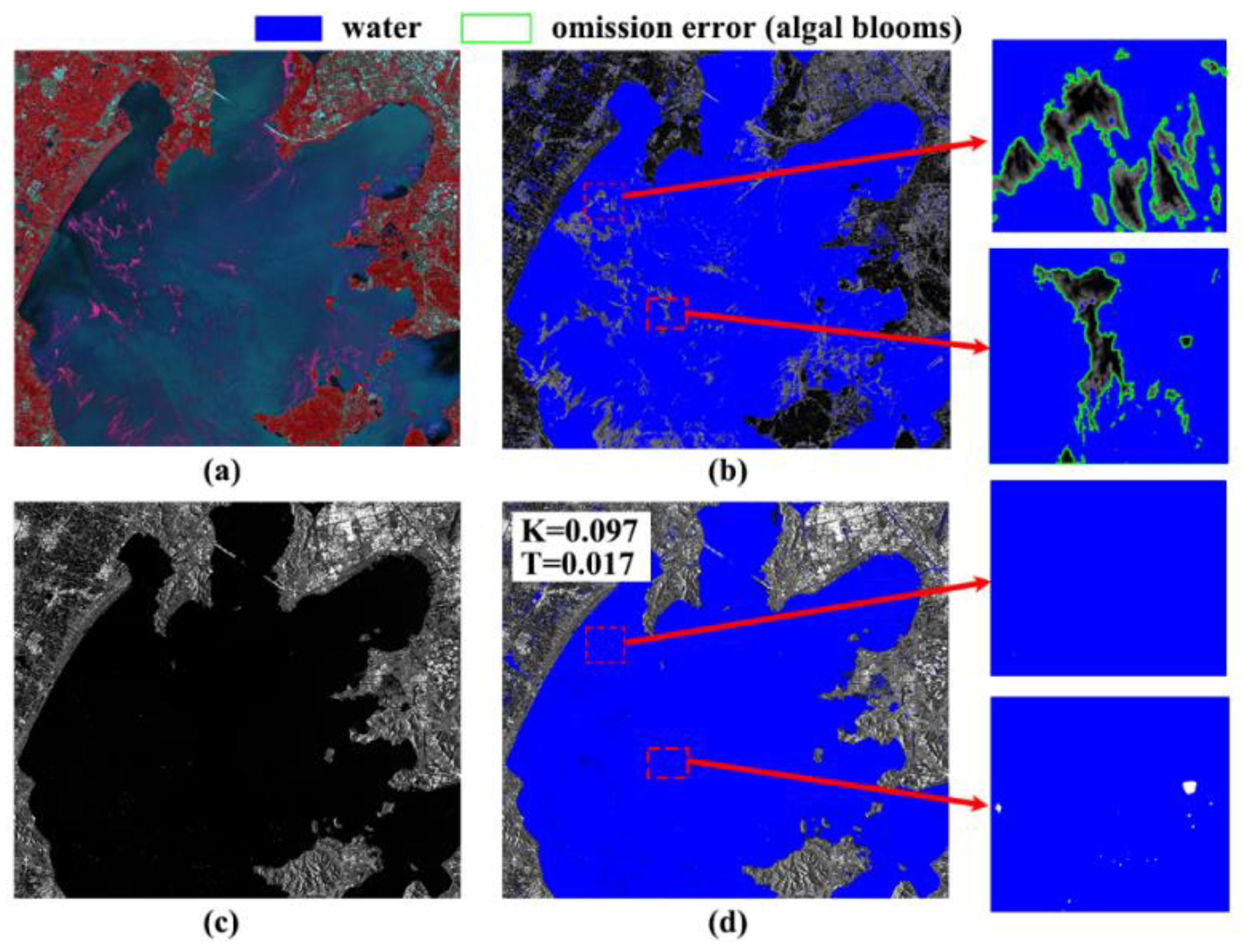
5.2. Waterbodies Covered by Algal Blooms

In the visible light band, the spectral characteristics of water are very complex, and thus, its reflectivity mainly depends on the reflection of the water surface and substances in the water. If the surface of the waterbody is covered by dense vegetation, such as algal blooms, the reflectance of the waterbody’s near-infrared band will be abnormally high and the water index based on the spectral characteristics of the waterbody will be seriously disturbed, and thus, the bloom-covered portion of the waterbody will be mistakenly classified as a non-water surface, resulting in omission. In recent years, with the intensification of human interference to the ecological environment, the temporal frequency and spatial scope of algal bloom outbreaks are on the rise, while a typical bloom can last for 6–8 months, covering the surface of the waterbody, thereby causing great interference to the statistics and estimation of water resources. As shown in Figure 9, when algal blooms erupted in the Taihu Lake area, the optical image could only extract the waterbody in the area without algal blooms, so it was difficult to monitor the changes of the Taihu Lake waterbody area over a long period of time. SAR images, on the other hand, have strong penetrating ability and can penetrate a certain degree of blooms, thereby more accurately reflecting the backscattering characteristics of waterbodies covered by blooms. Therefore, the SOWI algorithm integrated with SAR images could correctly obtain the distribution of waterbodies in Taihu Lake under the coverage of algal blooms, thus providing a reliable reference for water resource monitoring and waterbody protection in the Taihu Lake region.

5.3. Uneven Water and Smooth Terrain
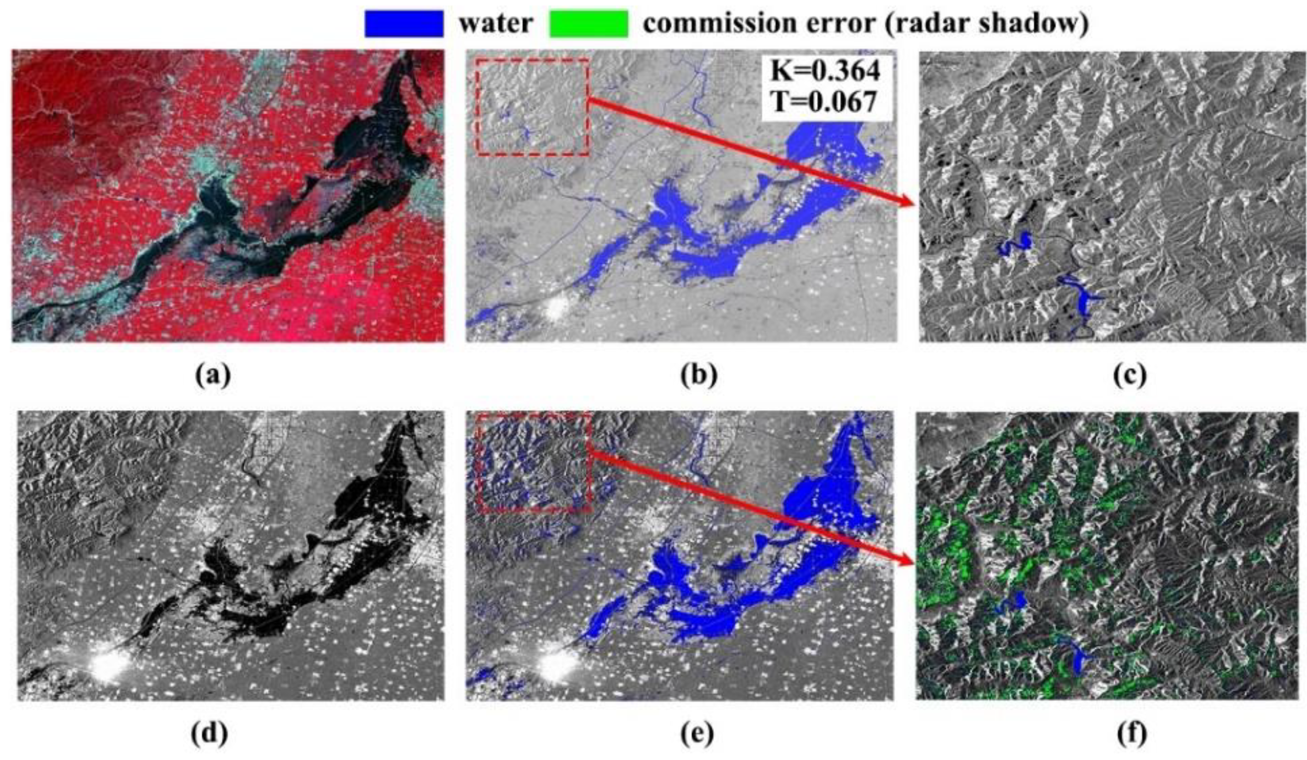
Strong winds increase the roughness of the water surface, which interferes with the SAR sensor signal and reduces the retroreflection gap between water and land [47]. In the inland areas of northwest China, the ground objects are mainly deserts with smooth surface, and the backward coefficient of non-water objects in SAR images is small. At the same time, the windy weather in these areas is frequent, and the backscattering mode of the waterbody is changed, which shows a higher gray value in the SAR image. For the studied area, the backscattering coefficients between land and water in SAR images were relatively close, making it difficult to extract water. As shown in Figure 10, Ulan-Ula Lake could not be identified as a waterbody by the SAR image, and only a small area of lakes surrounding it could be normally identified as such. Moreover, the larger the waterbody is, the easier it is to generate waves under the effect of strong wind, and Ulan-Ula Lake has a vast area. Thus, when the wind speed on the lake surface was high, a large number of waves were generated, increasing its backscattering coefficient in the SAR images. In contrast, the lakes around Ulan-Ula Lake have a smaller area, and thus, wave generation is difficult. Those water surfaces were relatively stable and the backscattering coefficient of the waterbody remained unchanged. Therefore, in contrast to the small surrounding lakes, Ulan-Ula Lake could not be correctly identified as a waterbody in the SAR images. Even with the effects of strong wind, the spectral characteristics of pure water do not generally change significantly. Wulan Wula Lake is generally less affected by human activities, and the waterbody is relatively pure because of the low content of planktic algae and sediment [48]. Therefore, the spectral characteristics of the waterbody of this lake did not change significantly due to the influence of wind and waves, and the extraction accuracy of NDWI and SOWI were both high. Since the SAR image in this area had high interference, there was no obvious double peak in the grayscale histogram. As shown in Figure 10 and Figure 11, different thresholds were set for the waterbody extracted from the SAR image. Compared with Figure 10, the threshold range was expanded during the process of waterbody extraction from the SAR image in Figure 11, yet there remained a high number of waterbodies in Ulan-Ula Lake that could not be extracted. At the same time, due to the expansion of the threshold range, smooth ground objects, such as the Gobi Desert and sediment in the Ulan-Ula Lake area, were mistakenly identified as waterbodies, and it was difficult to obtain the correct distribution range of waterbodies by using SAR images in this area. Overall, it is demonstrated that the SOWI algorithm can distinguish uneven water and smooth terrain in the conditions of strong wind by using the spectral features of the surface features.

5.4. Radar Shadow

The principle of side-view imaging of SAR images causes radar beams to be blocked by tall objects, such as mountains or buildings, and the resulting shadows in the images have a huge impact on SAR image data extraction, making it highly challenging to accurately extract waterbodies. Moreover, the backscatter value of the radar shadow area is located very close to the waterbody, and thus, the SAR image can easily mistake that area as the waterbody itself.
The imaging mode of optical images differs from that of SAR images [46]. Therefore, optical images tend to correctly reflect the spectral characteristics of ground objects in the radar shadow area. As shown in Figure 12, due to the occlusion of the mountain, the SAR image incorrectly extracts a large number of radar shadow areas as waterbodies, which would seriously affect the judgment of a disaster situation during flood monitoring, and thereby, limits its application in that field. In contrast, the SOWI algorithm can effectively reduce the misidentification of radar shadow areas as waterbodies and can accurately identify the distribution range of waterbodies during flood outbreaks.

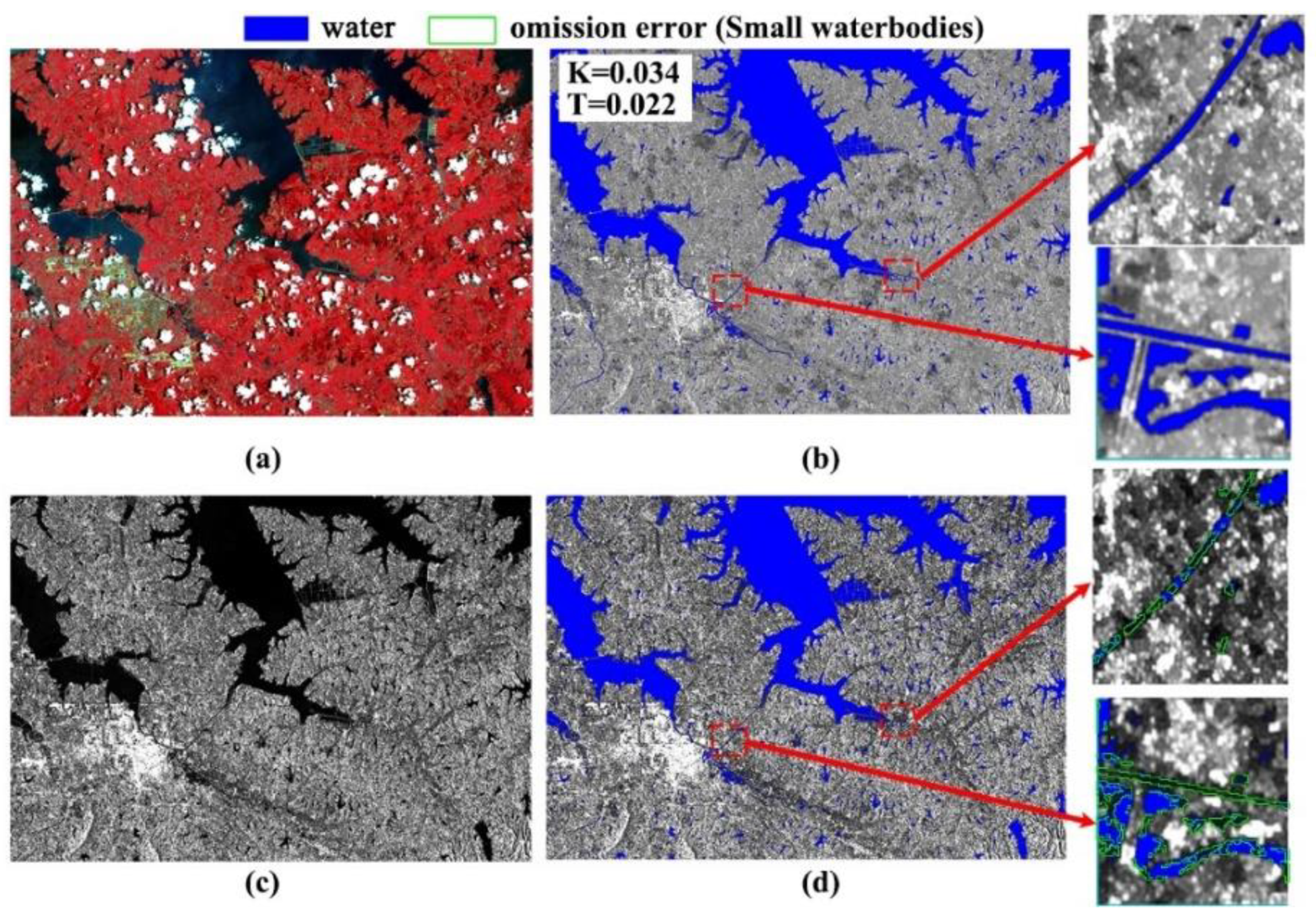
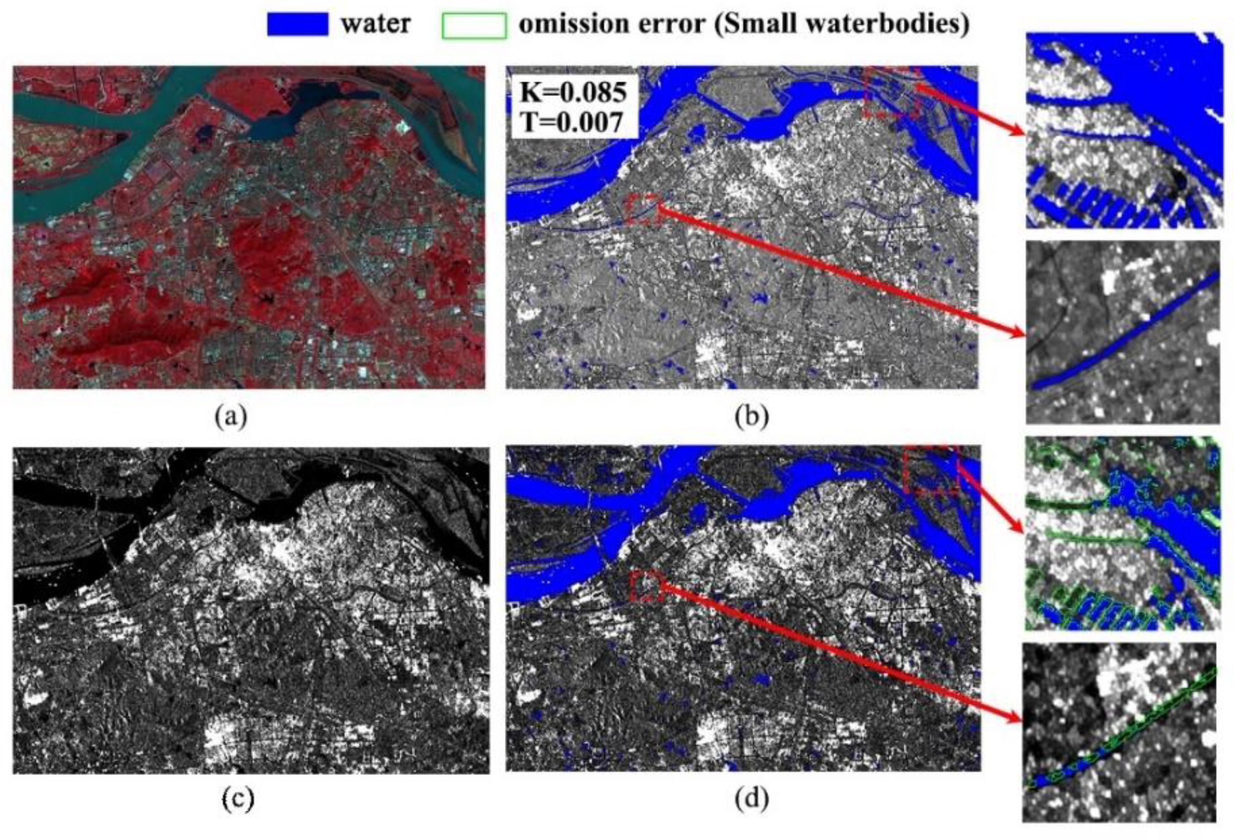
5.5. Small Waterbodies
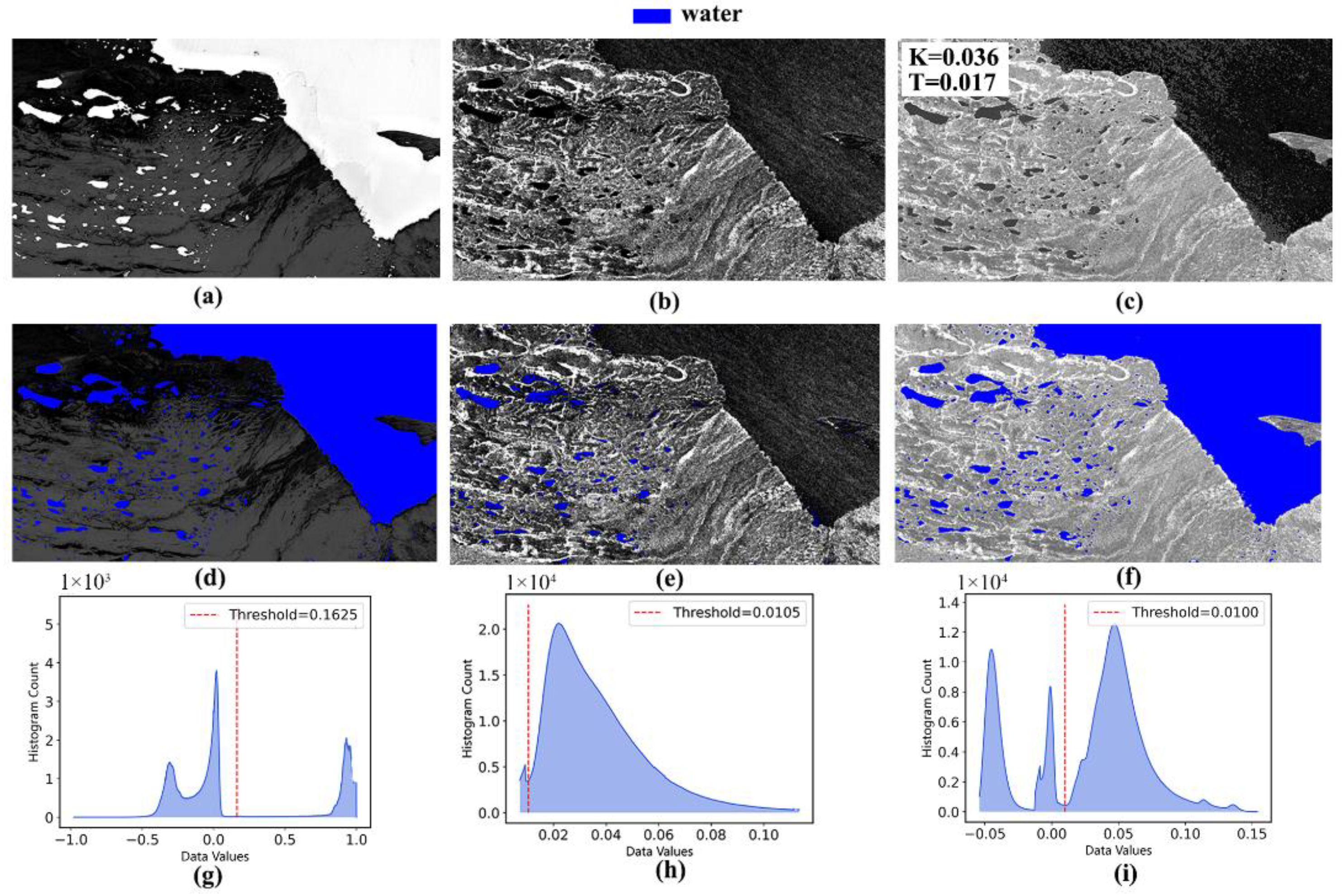
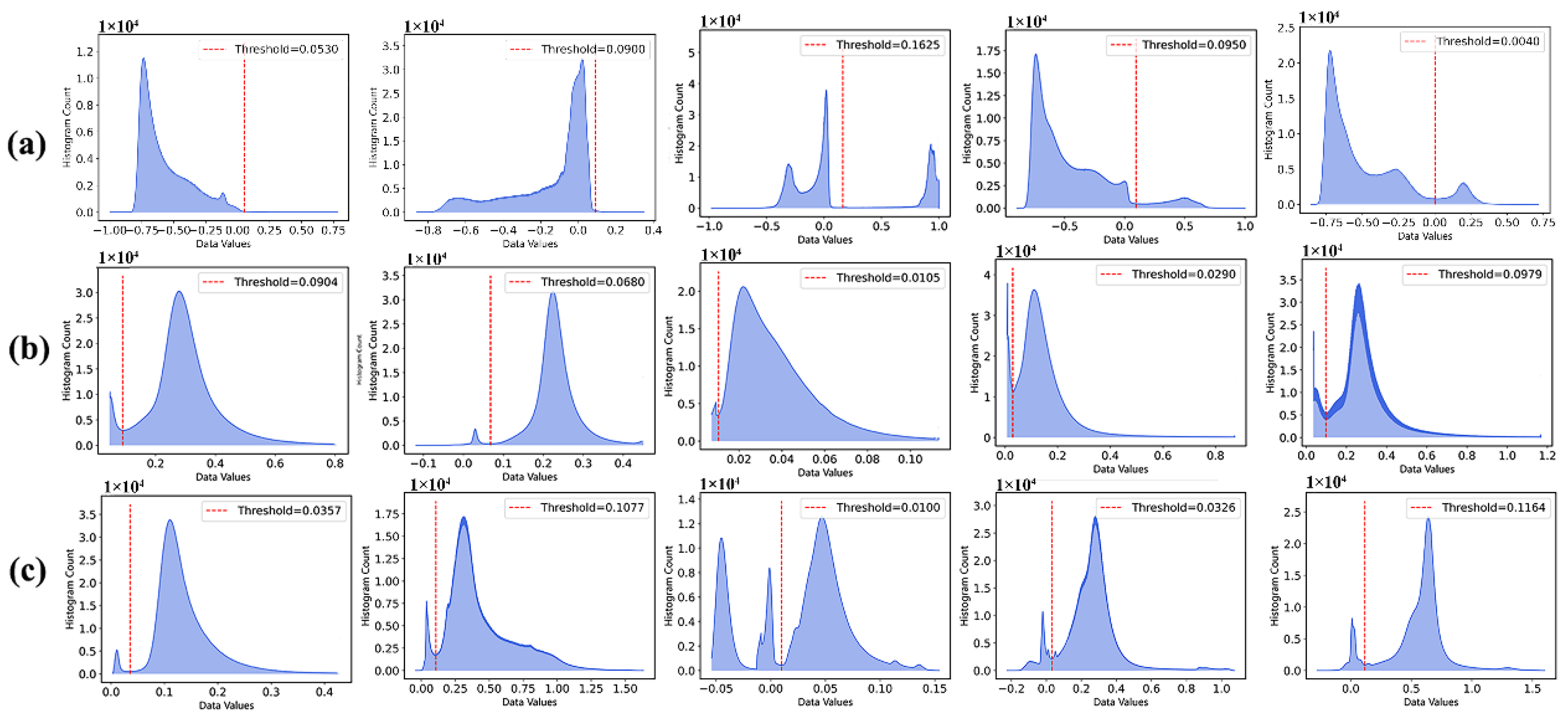
SAR images have lower spatial resolution and more noise, resulting in poor extraction of small waterbodies [10,46]. To date, most of the waterbody information extraction methods for SAR images have been developed for medium- and low-resolution images for large-area applications, and are not suitable for high-accuracy waterbody extraction. In addition, the asphalt pavement and building shadows in urban areas are similar to the backscattering characteristics of waterbodies, resulting in a serious decline in the accuracy of waterbody extraction from SAR images. Optical images have a higher spatial resolution and are richer in spectral information, therefore they can more effectively extract small waterbodies. Figure 13 and Figure 14 show the extraction of waterbodies under two different surface coverage conditions of lake waterbodies and urban waterbodies. The SOWI algorithm can effectively extract small rivers and pools that are difficult to identify in SAR images.

5.6. Histogram

The spectral characteristics of the waterbody are greatly disturbed by the substances on the surface and at the bottom of the water. Different suspended matter content in the waterbody, as well as different vegetation coverage on the water surface and different freezing conditions, surface backgrounds, and sediment contents all tend to lead to large spectral differences in waterbodies. The optimal threshold of the water index based on the spectral characteristics of water varies greatly. In the process of using the waterbody index to obtain the waterbody range, it has long been difficult to determine the optimal threshold [49]. SAR images are affected by speckle noise and uneven grayscale information throughout the image. At the same time, radar shadows are also present and the grayscale of smooth ground objects tends to be similar or identical to that of waterbodies. Thus, it is difficult to obtain accurate threshold points. The SOWI algorithm takes advantage of the different imaging mechanisms of both optical and SAR images, and uses the spectral characteristics and backscattering characteristics of ground objects to increase the difference between water and non-water objects. Compared with the frequency distribution histograms of NDWI and SAR images, the SOWI histogram exhibits notable peaks and valleys, as shown in Figure 15, which make it easier to identify a suitable threshold for the water extraction, and thus, greatly simplify the water extraction.

5.7. Precision Analysis of Different SOWI Types

When the data meet the requirements of SOWI, the MNDWI or NDWI are selected according to the requirements and combined with the VV or HH polarization of the SAR image to extract the waterbody. In general, the water extraction accuracy of SOWI combined with MNDWI or NDWI is generally close, and in most cases, its effect combined with MNDWI is slightly better. Figure 16 shows that the water extraction accuracy of the SOWI algorithm combined with MNDWI is better than that of SOWI combined with NDWI in Yangzhou, the Dongming section of the Yellow River in Shandong, and Taihu Lake. The Ulan-Ula Lake area contains a large amount of snow, which leads to a larger absorption minimum close to the 1400 nm band [50]. The MNDWI calculated based on Sentinel-2 data misjudges snow as waterbody, resulting in a significantly weaker extraction accuracy of the SOWI algorithm combined with MNDWI compared with that of the SOWI algorithm combined with NDWI.

5.8. Limitations of SOWI

The SOWI algorithm has two main limitations. First, the construction of SOWI algorithm requires the SAR image and optical image with close dates. When the date difference between the two is more than 30 days, the water range of the two may change significantly, which reduces the accuracy of the extraction results. Fortunately, as more satellites are launched and satellite data from various regions become more abundant, it will be increasingly easier to obtain optical and SAR images of the same area with similar dates. Second, although the SOWI algorithm makes use of the complementary advantages of the two data types to improve the accuracy of water extraction, if neither of them can obtain water information in a given area, the extraction accuracy is low. For example, when there is disturbance of both wind waves and algal blooms at the same time on the lake surface, or if the radar shadow area is blocked by clouds and fog, the results of water extraction may be inaccurate.

6. Conclusions

This paper develops a novel waterbody index (SOWI) combining SAR and optical imagery to classify waterbody and non-waterbody areas. The proposed waterbody index utilizes the advantages and disadvantages of each sensor, and can perform high-precision waterbody extraction in a variety of scenarios by increasing the difference between waterbody and non-waterbody pixels and reducing the difficulty of threshold determination. The SOWI uses the principles of the optical image water index and SAR image thresholding method to extract waterbody distribution; fusing NDWI, MNDWI, and other waterbody indices with SAR image co-polarization bands to perform calculations. Moreover, it combines different features of the two image types to better highlight waterbody information for quicker and more accurate determination of the distribution of waterbodies.
In this study, the SOWI algorithm combining NDWI and VV polarization bands was tested in five research areas. The average producer accuracy of the water extraction results in the five areas was 89%, the average user accuracy was 98%, the average overall accuracy was 97%, and the average Kappa coefficient was 91%, all of which were better than the extraction methods based on SAR image or optical image. In addition, based on the SOWI algorithm, a time series map of waterbody distribution during the 2021 flood outbreak in Xunxian County, Henan Province was drawn. When the SOWI algorithm was used to form the sequence observations, the change detection method was successful in automatically and accurately extracting the flood range. Based on this performance, we conclude that the SOWI algorithm can be used as a method of flood disaster monitoring, as it automatically and accurately obtains the distribution range of flood waters, thereby providing effective information for rescue and relief after a flood outbreak. Moreover, the SOWI algorithm can also be used to accurately determine regional waterbody distribution, as well as to create a long-term regional water distribution map. It is of great significance for water resource statistics and water environmental protection in areas that are affected by monsoon climate and long-term cloud and fog coverage.

Author Contributions

Conceptualization, B.T., F.Z. and F.L.; methodology, B.T. and F.Z.; software, B.T.; validation, C.W. (Chen Wang) and S.W.; formal analysis, F.L. and C.W. (Chao Wang); investigation, C.W. (Chen Wang); resources, J.L.; data curation, B.T.; writing—original draft preparation, B.T.; writing—review and editing, B.T.; visualization, F.Z.; supervision, S.W.; project administration, F.Z.; funding acquisition, F.Z. All authors have read and agreed to the published version of the manuscript.

Funding

This work was supported in part by the Strategic Priority Research Program of the Chinese Academy of Sciences (No. XDA19080304) and the Major Research Focus project of the Henan Academy of Sciences (No. 210101007).

Data Availability Statement

Not applicable.

Acknowledgments

The authors would like to thank the Institute of Remote Sensing and Digital Earth, Chinese Academy of Sciences and Geospatial Data Cloud for providing GF images and the European Space Agency for providing the Sentinel-2 MSI data.

Conflicts of Interest

The authors declare no conflict of interest.

References

  1. Druce, D.; Tong, X.Y.; Lei, X.; Guo, T.; Kittel, C.M.M.; Grogan, K.; Tottrup, C. An Optical and SAR Based Fusion Approach for Mapping Surface Water Dynamics over Mainland China. Remote Sens. 2021, 13, 1663. [Google Scholar] [CrossRef]
  2. Irwin, K.; Beaulne, D.; Braun, A.; Fotopoulos, G. Fusion of SAR, Optical Imagery and Airborne LiDAR for Surface Water Detection. Remote Sens. 2017, 9, 890. [Google Scholar] [CrossRef] [Green Version]
  3. Raymond, P.A.; Hartmann, J.; Lauerwald, R.; Sobek, S.; McDonald, C.; Hoover, M.; Butman, D.; Striegl, R.; Mayorga, E.; Humborg, C.; et al. Global carbon dioxide emissions from inland waters. Nature 2013, 503, 355–359. [Google Scholar] [CrossRef] [PubMed] [Green Version]
  4. Huang, W.L.; DeVries, B.; Huang, C.Q.; Lang, M.W.; Jones, J.W.; Creed, I.F.; Carroll, M.L. Automated Extraction of Surface Water Extent from Sentinel-1 Data. Remote Sens. 2018, 10, 797. [Google Scholar] [CrossRef] [Green Version]
  5. Gasparovic, M.; Klobucar, D. Mapping Floods in Lowland Forest Using Sentinel-1 and Sentinel-2 Data and an Object-Based Approach. Forests 2021, 12, 553. [Google Scholar] [CrossRef]
  6. Senay, G.B.; Schauer, M.; Friedrichs, M.; Velpuri, N.M.; Singh, R.K. Satellite-based water use dynamics using historical Landsat data (1984-2014) in the southwestern United States. Remote Sens. Environ. 2017, 202, 98–112. [Google Scholar] [CrossRef]
  7. Wang, C.; Jia, M.M.; Chen, N.C.; Wang, W. Long-Term Surface Water Dynamics Analysis Based on Landsat Imagery and the Google Earth Engine Platform: A Case Study in the Middle Yangtze River Basin. Remote Sens. 2018, 10, 1635. [Google Scholar] [CrossRef] [Green Version]
  8. Zhao, W. Phase research and practice of upgrading earth observation from test application to system effectiveness in China. J. Remote Sens. 2019, 23, 1036–1045. [Google Scholar]
  9. Zhang, Y.J.; Liu, X.Y.; Zhang, Y.; Ling, X.; Huang, X. Automatic and Unsupervised Water Body Extraction Based on Spectral-Spatial Features Using GF-1 Satellite Imagery. IEEE Geosci. Remote Sens. Lett. 2019, 16, 927–931. [Google Scholar] [CrossRef]
  10. Dan, L.; Baosheng, W.; Bowei, C.; Yuan, X.; Yi, Z. Review of water body information extraction based on satellite remote sensing. J. Tsinghua Univ. 2020, 60, 147–161. [Google Scholar] [CrossRef]
  11. Slinski, K.M.; Hogue, T.S.; McCray, J.E. Active-Passive Surface Water Classification: A New Method for high-Resolution monitoring of Surface Water Dynamics. Geophys. Res. Lett. 2019, 46, 4694–4704. [Google Scholar] [CrossRef]
  12. Deng, Y.; Jiang, W.G.; Tang, Z.H.; Li, J.H.; Lv, J.X.; Chen, Z.; Jia, K. Spatio-Temporal Change of Lake Water Extent in Wuhan Urban Agglomeration Based on Landsat Images from 1987 to 2015. Remote Sens. 2017, 9, 270. [Google Scholar] [CrossRef] [Green Version]
  13. Zou, Z.H.; Xiao, X.M.; Dong, J.W.; Qin, Y.W.; Doughty, R.B.; Menarguez, M.A.; Zhang, G.L.; Wang, J. Divergent trends of open-surface water body area in the contiguous United States from 1984 to 2016. Proc. Natl. Acad. Sci. USA 2018, 115, 3810–3815. [Google Scholar] [CrossRef] [Green Version]
  14. Sharma, R.C.; Tateishi, R.; Hara, K.; Nguyen, L.V. Developing Superfine Water Index (SWI) for Global Water Cover Mapping Using MODIS Data. Remote Sens. 2015, 7, 13807–13841. [Google Scholar] [CrossRef] [Green Version]
  15. Feyisa, G.L.; Meilby, H.; Fensholt, R.; Proud, S.R. Automated Water Extraction Index: A new technique for surface water mapping using Landsat imagery. Remote Sens. Environ. 2014, 140, 23–35. [Google Scholar] [CrossRef]
  16. Bing, Z.; Junsheng, L.; Qian, S.; Yanhong, W.; Fangfang, Z.; Shenglei, W.; Yue, Y.; Linan, G.; Ziyao, Y. Recent research progress on long time series and large scale optical remote sensing of inland water. J. Remote Sens. 2021, 25, 37–52. [Google Scholar]
  17. Yuchen, L.; Yongnian, G. Surface water extraction in Yangtze River Basin based on sentinel time series image. J. Remote Sens. 2022, 26, 358–372. [Google Scholar]
  18. Kaplan, G.; Avdan, U. Object-based water body extraction model using Sentinel-2 satellite imagery. Eur. J. Remote Sens. 2017, 50, 137–143. [Google Scholar] [CrossRef] [Green Version]
  19. Jones, J.W. Efficient Wetland Surface Water Detection and Monitoring via Landsat: Comparison with in situ Data from the Everglades Depth Estimation Network. Remote Sens. 2015, 7, 12503–12538. [Google Scholar] [CrossRef] [Green Version]
  20. Zhang, G.Q.; Zheng, G.X.; Gao, Y.; Xiang, Y.; Lei, Y.B.; Li, J.L. Automated Water Classification in the Tibetan Plateau Using Chinese GF-1 WFV Data. Photogramm. Eng. Remote Sens. 2017, 83, 509–519. [Google Scholar] [CrossRef]
  21. McFeeters, S.K. The use of the normalized difference water index (NDWI) in the delineation of open water features. Int. J. Remote Sens 1996, 17, 1425–1432. [Google Scholar] [CrossRef]
  22. Xu, H. Modification of normalised difference water index (NDWI) to enhance open water features in remotely sensed imagery. J. Remote Sens. 2005, 27, 589–595. [Google Scholar] [CrossRef]
  23. Kaiyuan, D.; Chao, R. Water extraction model of multispectral optical remote sensing image. Acta. Geod. Et. Cartogr. Sin. 2021, 50, 1370–1379. [Google Scholar]
  24. Zhou, Y.A.; Luo, J.C.; Shen, Z.F.; Hu, X.D.; Yang, H.P. Multiscale Water Body Extraction in Urban Environments from Satellite Images. IEEE J-Stars 2014, 7, 4301–4312. [Google Scholar] [CrossRef]
  25. Ahmad, S.K.; Hossain, F.; Eldardiry, H.; Pavelsky, T.M. A Fusion Approach for Water Area Classification Using Visible, Near Infrared and Synthetic Aperture Radar for South Asian Conditions. IEEE Trans Geosci Remote Sens. 2020, 58, 2471–2480. [Google Scholar] [CrossRef]
  26. Grimaldi, S.; Xu, J.; Li, Y.; Pauwels, V.R.N.; Walker, J.P. Flood mapping under vegetation using single SAR acquisitions. Remote Sens. Environ. 2020, 237, 111582. [Google Scholar] [CrossRef]
  27. Liang, J.Y.; Liu, D.S. A local thresholding approach to flood water delineation using Sentinel-1 SAR imagery. ISPRS J. Photogramm 2020, 159, 53–62. [Google Scholar] [CrossRef]
  28. Shen, X.Y.; Wang, D.C.; Mao, K.B.; Anagnostou, E.; Hong, Y. Inundation Extent Mapping by Synthetic Aperture Radar: A Review. Remote Sens. 2019, 11, 879. [Google Scholar] [CrossRef] [Green Version]
  29. Liu, X.Y.; Liu, L.; Shao, Y.; Zhao, Q.H.; Zhang, Q.J.; Lou, L.J. Water Detection in Urban Areas from GF-3. Sensors 2018, 18, 1299. [Google Scholar] [CrossRef] [Green Version]
  30. Prigent, C.; Matthews, E.; Aires, F.; Rossow, W.B. Remote sensing of global wetland dynamics with multiple satellite data sets. Geophys. Res. Lett. 2001, 28, 4631–4634. [Google Scholar] [CrossRef] [Green Version]
  31. White, L.; Brisco, B.; Dabboor, M.; Schmitt, A.; Pratt, A. A Collection of SAR Methodologies for Monitoring Wetlands. Remote Sens. 2015, 7, 7615–7645. [Google Scholar] [CrossRef] [Green Version]
  32. Wang, G.L. Active and Passive Remote Sensing Monitoring of Cyanobacterial Blooms in Inland Waters; East China Normal University: Shanghai, China, 2015. [Google Scholar]
  33. Zeng, C.Q.; Wang, J.F.; Huang, X.D.; Bird, S.; Luce, J.J. Urban water body detection from the combination of high-resolution optical and SAR images. In Proceedings of the JURSE, Lausanne, Switzerland, 30 March–1 April 2015. [Google Scholar]
  34. Hong, S.; Jang, H.; Kim, N.; Sohn, H.G. Water Area Extraction Using RADARSAT SAR Imagery Combined with Landsat Imagery and Terrain Information. Sensors 2015, 15, 6652–6667. [Google Scholar] [CrossRef] [PubMed]
  35. Long, J.; Ding, X.; Wang, C. Complex Coherence Estimation Based on Adaptive Refined Lee Filter. Acta Geod. Et Cartogr. Sin. 2015, 44, 1331–1339. [Google Scholar]
  36. Jiang, W.H.; Yu, A.X.; Dong, Z.; Wang, Q.S. Comparison and Analysis of Geometric Correction Models of Spaceborne SAR. Sensors 2016, 16, 973. [Google Scholar] [CrossRef]
  37. Twele, A.; Cao, W.X.; Plank, S.; Martinis, S. Sentinel-1-based flood mapping: A fully automated processing chain. Int. J. Remote Sens. 2016, 37, 2990–3004. [Google Scholar] [CrossRef]
  38. Clement, M.A.; Kilsby, C.G.; Moore, P. Multi-temporal synthetic aperture radar flood mapping using change detection. J. Flood Risk Manag. 2018, 11, 152–168. [Google Scholar] [CrossRef] [Green Version]
  39. Wang, G.; Wu, M.; Wei, X.; Song, H. Water Identification from High-Resolution Remote Sensing Images Based on Multidimensional Densely Connected Convolutional Neural Networks. Remote Sens. 2020, 12, 795. [Google Scholar] [CrossRef] [Green Version]
  40. Jiang, W.; He, G.; Long, T.; Ni, Y.; Liu, H.; Peng, Y.; Lv, K.; Wang, G. Multilayer Perceptron Neural Network for Surface Water Extraction in Landsat 8 OLI Satellite Images. Remote Sens. 2018, 10, 755. [Google Scholar] [CrossRef] [Green Version]
  41. Rogers, A.S.; Kearney, M.S. Reducing signature variability in unmixing coastal marsh Thematic Mapper scenes using spectral indices. Int. J. Remote Sens. 2004, 25, 2317–2335. [Google Scholar] [CrossRef]
  42. Chen, L.F.; Zhang, P.; Xing, J.; Li, Z.H.; Xing, X.M.; Yuan, Z.H. A Multi-Scale Deep Neural Network for Water Detection from SAR Images in the Mountainous Areas. Remote Sens. 2020, 12, 3205. [Google Scholar] [CrossRef]
  43. Fan, K.G.; Huang, W.G.; He, M.X.; Fu, B.; Zhang, B.; Chen, X.Y. Depth inversion in coastal water based on SAR image of waves. Chin. J. Oceanol. Limnol. 2008, 26, 434–439. [Google Scholar] [CrossRef]
  44. Zhang, F.; Li, J.; Zhang, B.; Shen, Q.; Ye, H.; Wang, S.; Lu, Z. A simple automated dynamic threshold extraction method for the classification of large water bodies from landsat-8 OLI water index images. Int. J. Remote Sens. 2018, 39, 3429–3451. [Google Scholar] [CrossRef]
  45. Wu, Q.S.; Wang, M.X.; Shen, Q.; Yao, Y.; Li, J.S.; Zhang, F.F.; Zhou, Y.M. Small water body extraction method based on Sentinel-2 satellite multi-spectral remote sensing image. Natl. Remote Sens. Bull. 2022, 26, 781–794. [Google Scholar] [CrossRef]
  46. Gu, X.; Zeng, Q.; Shen, H.; Chen, E.; Zhao, L.; Yu, F.; Tu, K. Study on water information extraction using domestic GF-3 image. J. Remote Sens. 2019, 23, 555–565. [Google Scholar]
  47. White, L.; Brisco, B.; Pregitzer, M.; Tedford, B.; Boychuk, L. RADARSAT-2 Beam Mode Selection for Surface Water and Flooded Vegetation Mapping. Can. J. Remote Sens. 2014, 40, 135–151. [Google Scholar] [CrossRef]
  48. Yan, Q.; Liao, J.J.; Shen, G.Z. Remote sensing analysis and simulation of change of Ulan Ul Lake in the past 40 years. Remote Sens. Land Resour. 2014, 26, 152–157. [Google Scholar]
  49. Ji, L.; Zhang, L.; Wylie, B. Analysis of Dynamic Thresholds for the Normalized Difference Water Index. Photogramm. Eng. Remote Sens. 2009, 75, 1307–1317. [Google Scholar] [CrossRef]
  50. Qunzhu, Z.; Meisheng, C.; Wenkun, S. Study on the spectral characteristics of the snow layer moisture content in the snowmelt period on the northern slope of Tianshan Mountains. Spectrosc Spect. Anal. 2013, 33, 2177–2181. [Google Scholar]
Figure 1. Spatial distribution of the research areas over China used for testing the SAR and Optical Imagery Water Index (SOWI) in this study.
Remotesensing 14 05316 g001
Figure 2. Overview of the application of the fusion algorithm SOWI based on two different satellite images, that is, optical and synthetic aperture radar (SAR) images.
Remotesensing 14 05316 g002
Figure 3. Example of the calculation of the balance coefficient K: (a) SAR imagery. (b) Regions with small backscattering coefficients in the NDWI (blue area). (c) HH histogram (red line represents the threshold). (d) Regions with small backscattering coefficients in SAR imagery (blue area).
Remotesensing 14 05316 g003
Figure 4. Threshold T1 calculation example: (a) Normalized Difference Water Index (NDWI). (b) Histogram of NDWI (red line represents the threshold). (c) Determined as waterbody according to the threshold in the NDWI histogram (blue area). (d) The same waterbody in the SAR image (blue area). (e) Preliminary determination of the water area in SAR images according to T1 (green area).
Remotesensing 14 05316 g004
Figure 5. Time series change map of the flood inundation area in Xunxian County, Henan Province: (a) Optical image. (b) SAR image. (c) Water extraction from SAR image. (d) SOWI. (e) Water extraction from SOWI.
Remotesensing 14 05316 g005
Figure 6. The curve of the flood area with time obtained by the three algorithms during the flood outbreak period in Xunxian County, Henan Province.
Remotesensing 14 05316 g006
Figure 7. Results of the water extraction in Xunxian County, Henan Province, under the occlusion of clouds and fog: (a) Optical image. (b) NDWI. (c) Water extraction results based on the NDWI. (d) SAR image. (e) SOWI. (f) Water extraction results based on the SOWI.
Remotesensing 14 05316 g007
Figure 8. Results of the water extraction in the Junshan Lake area under the occlusion of clouds and fog: (a) Optical image. (b) Water extraction based on the NDWI. (c) SAR image. (d) Water extraction based on the SOWI.
Remotesensing 14 05316 g008
Figure 9. Results of the water extraction in Taihu Lake under algal bloom conditions: (a) Optical image. (b) Water extraction based on the NDWI. (c) SAR image. (d) Water extraction based on the SOWI.
Remotesensing 14 05316 g009
Figure 10. Waterbody extraction map for the Ulan-Ula Lake area under strong wind: (a) NDWI. (b) HH. (c) SOWI. (d) Water extraction based on the NDWI. (e) Water extraction based on VV. (f) Water extraction based on the SOWI. (g) NDWI histogram. (h) VV histogram. (i) SOWI histogram. The red lines in (gi) represents the threshold.
Remotesensing 14 05316 g010
Figure 11. Waterbody extraction map for the for the Ulan-Ula Lake area under strong wind: (a) Optical image. (b) SAR image. (c) Water extraction based on the SOWI. (d) SOWI histogram. (e) Water extraction based on VV. (f) VV histogram. The red lines in (d,f) represent the threshold.
Remotesensing 14 05316 g011
Figure 12. Waterbody extraction map for Xunxian County, Henan Province, under radar shadow interference: (a) Optical image. (b) Water extraction based on the SOWI. (c) Partially enlarged view of the SOWI water extraction results. (d) SAR image. (e) Water extraction based on HH. (f) Partially enlarged view of the HH water extraction.
Remotesensing 14 05316 g012
Figure 13. Waterbody extraction map for the Junshan Lake area: (a) Optical image. (b) Water extraction based on the SOWI. (c) SAR image. (d) Water extraction based on VV.
Remotesensing 14 05316 g013
Figure 14. Waterbody extraction map for Yangzhou, Jiangsu: (a) Optical image. (b) Water extraction based on the SOWI. (c) SAR image. (d) Water extraction based on VV.
Remotesensing 14 05316 g014
Figure 15. Comparison of histograms: (a) NDWI. (b) Co-polar band. (c) SOWI. In each panel, the red line represents the threshold.
Remotesensing 14 05316 g015
Figure 16. Accuracy comparison of SOWI algorithm combined with NDWI and MNDWI in five study areas.
Remotesensing 14 05316 g016
Table 1. Description of Sentinel-1/2 scenes.
Test SiteAcquisition DateInterference
Sentinel-1Sentinel-2
Dongming section of the Yellow River in Shandong27 July 202126 July 2021Cloud
Junshan Lake9 June 20215 June 2021Small waterbody, Cloud
Yangzhou, Jiangsu1 August 20212 August 2021Small waterbody
Taihu Lake15 August 201917 August 2019Algal blooms, Radar shadow
Ulan-Ula Lake6 October 20217 October 2021Windy, Smooth terrain
Table 2. Summary of accuracy assessments at the five main test sites including various accuracy measurements.
SiteApproachOverall AccuracyUser AccuracyProducer AccuracyKappa Coefficient
Yangzhou, JiangsuNDWI0.96700.98880.79020.8596
VV0.95130.95350.71200.7878
S O W I 0.97080.98060.82310.8782
Junshan LakeNDWI0.96460.98540.82270.8756
VV0.97330.97360.88100.9088
S O W I 0.97730.97810.89840.9288
Dongming section of the Yellow River in ShandongNDWI0.97430.83680.08230.1457
VV0.99200.96140.73810.8311
SOWI0.99290.95470.77960.8547
Taihu LakeNDWI0.92330.99190.89120.8366
VV0.97070.96800.98840.9340
S O W I 0.98740.99770.98320.9721
Ulan-Ula LakeNDWI0.99000.99340.97460.9766
VV0.70750.95620.07270.0949
S O W I 0.98910.99390.97210.9747
Table 3. Summary of accuracy assessments for different dates in the case area, including various accuracy measurements.
DateApproachOverall AccuracyUser AccuracyProducer AccuracyKappa Coefficient
7.31NDWI0.9100.9360.8800.820
VV0.780.7590.8200.56
SOWI0.9050.9350.8700.81
8.08NDWI0.5900.9900.1450.151
VV0.8200.7940.8430.642
SOWI0.8800.8910.8540.759
Publisher’s Note: MDPI stays neutral with regard to jurisdictional claims in published maps and institutional affiliations.

