
A Google Earth Engine Approach for Wildfire Susceptibility Prediction Fusion with Remote Sensing Data of Different Spatial Resolutions


 ,
,  ,
,  and
and
Abstract
:1. Introduction
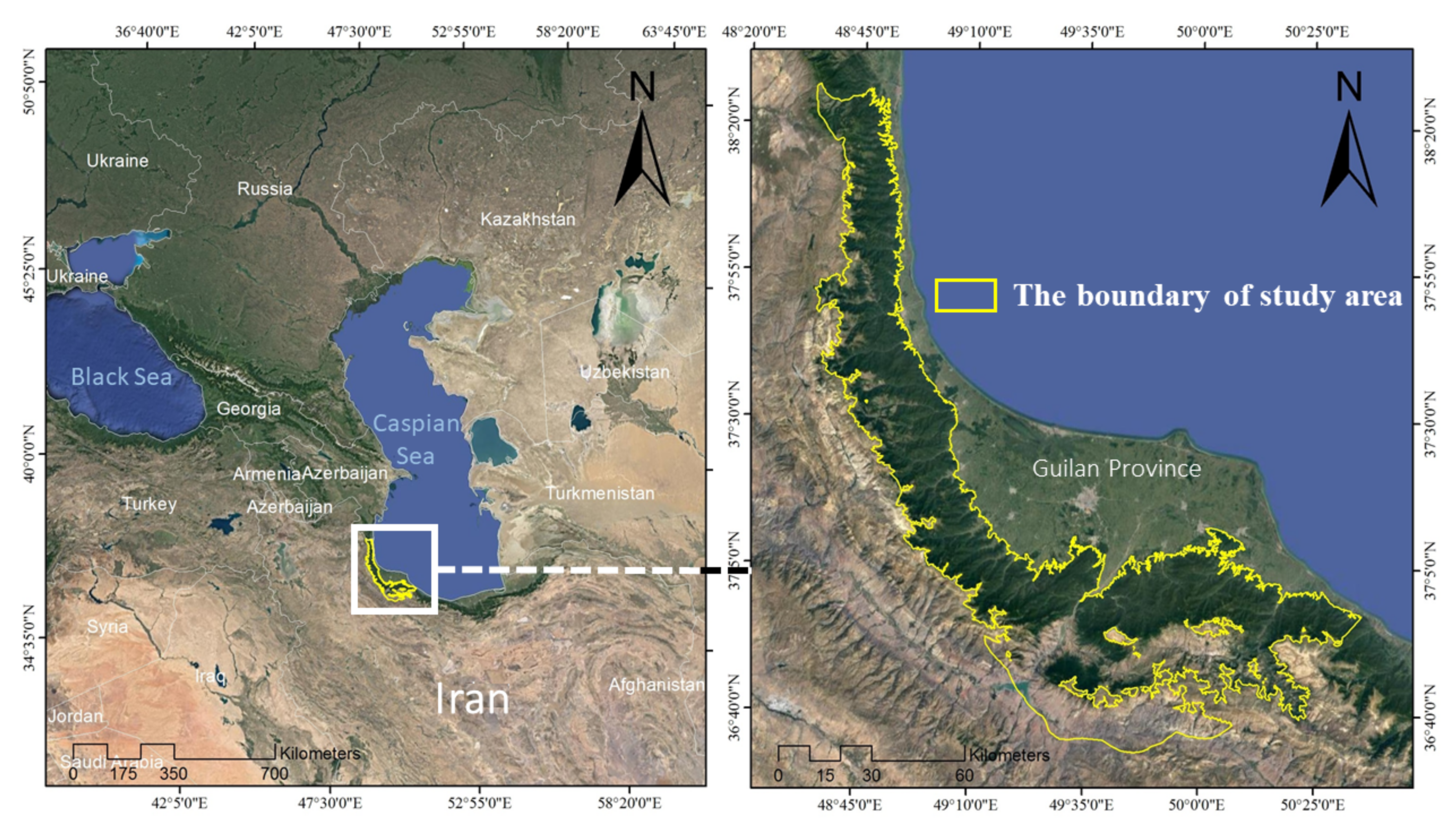
2. Study Area
3. Inventory and Conditioning Factors
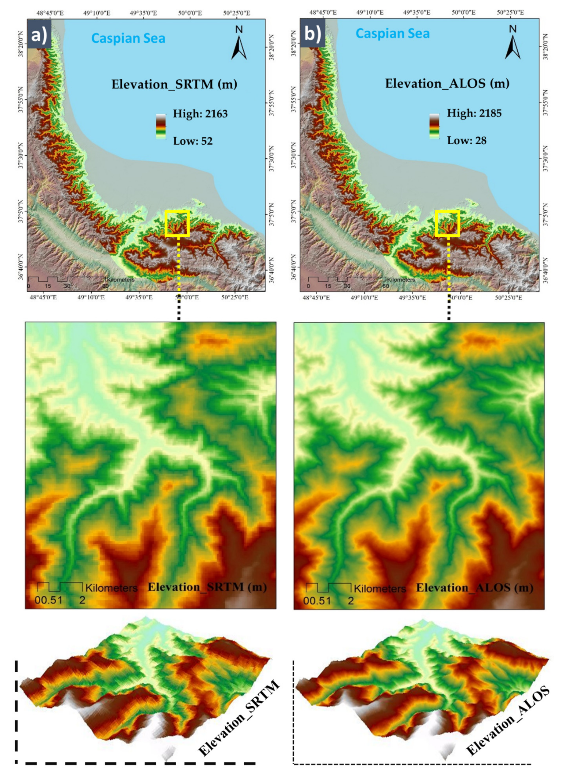
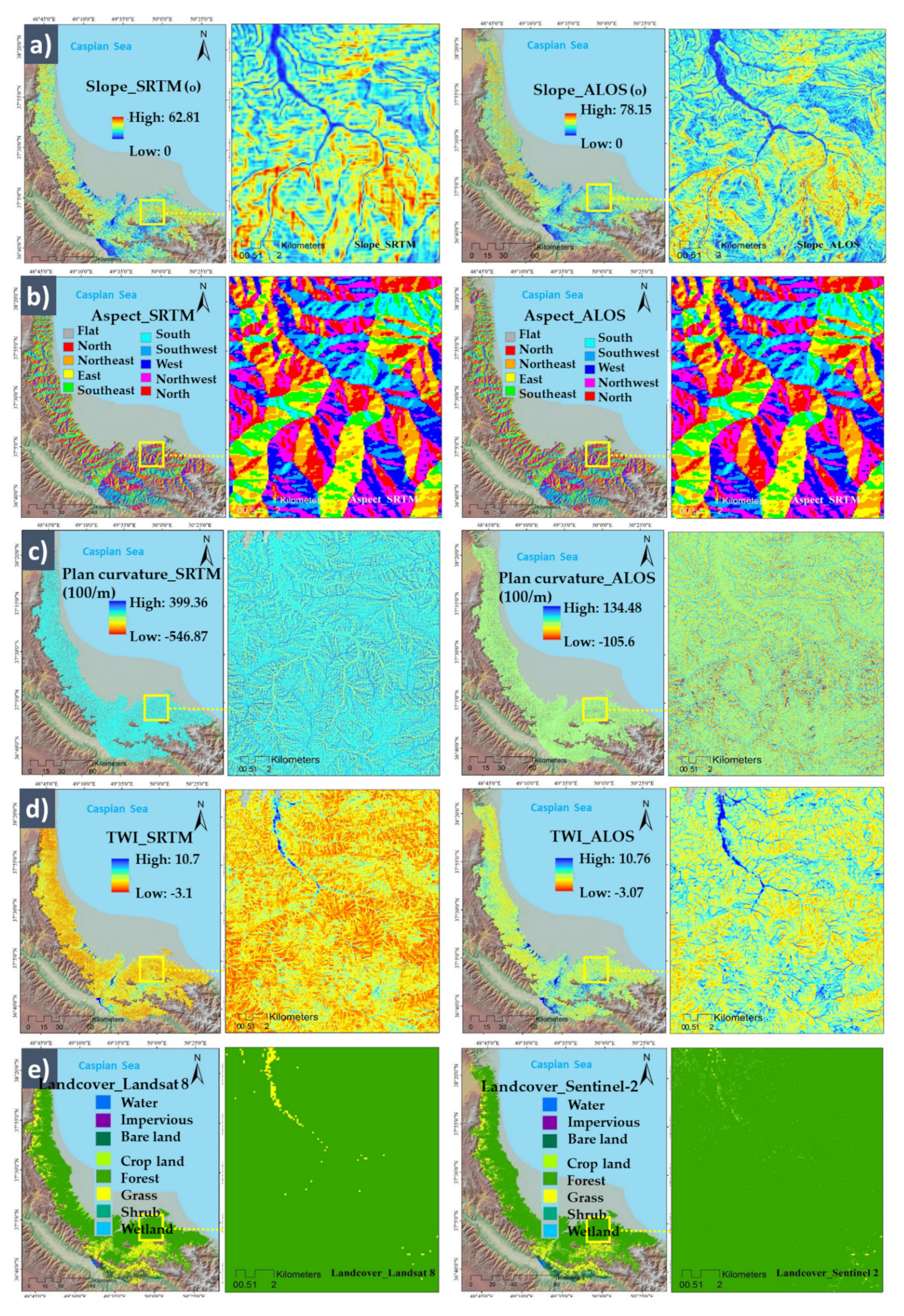
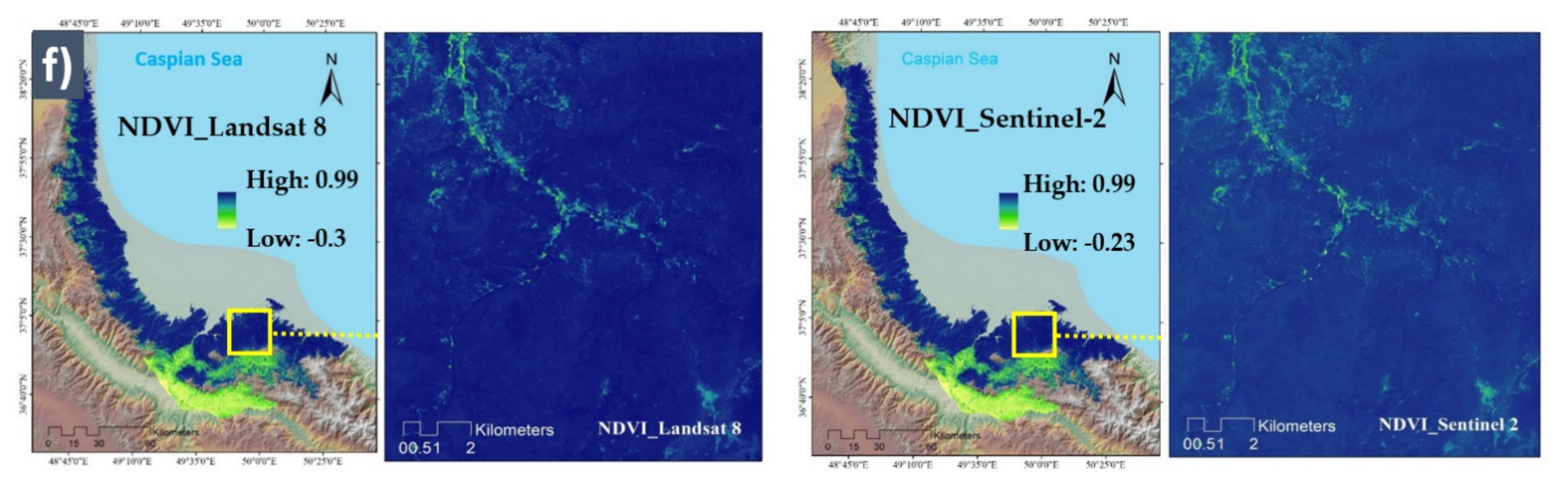
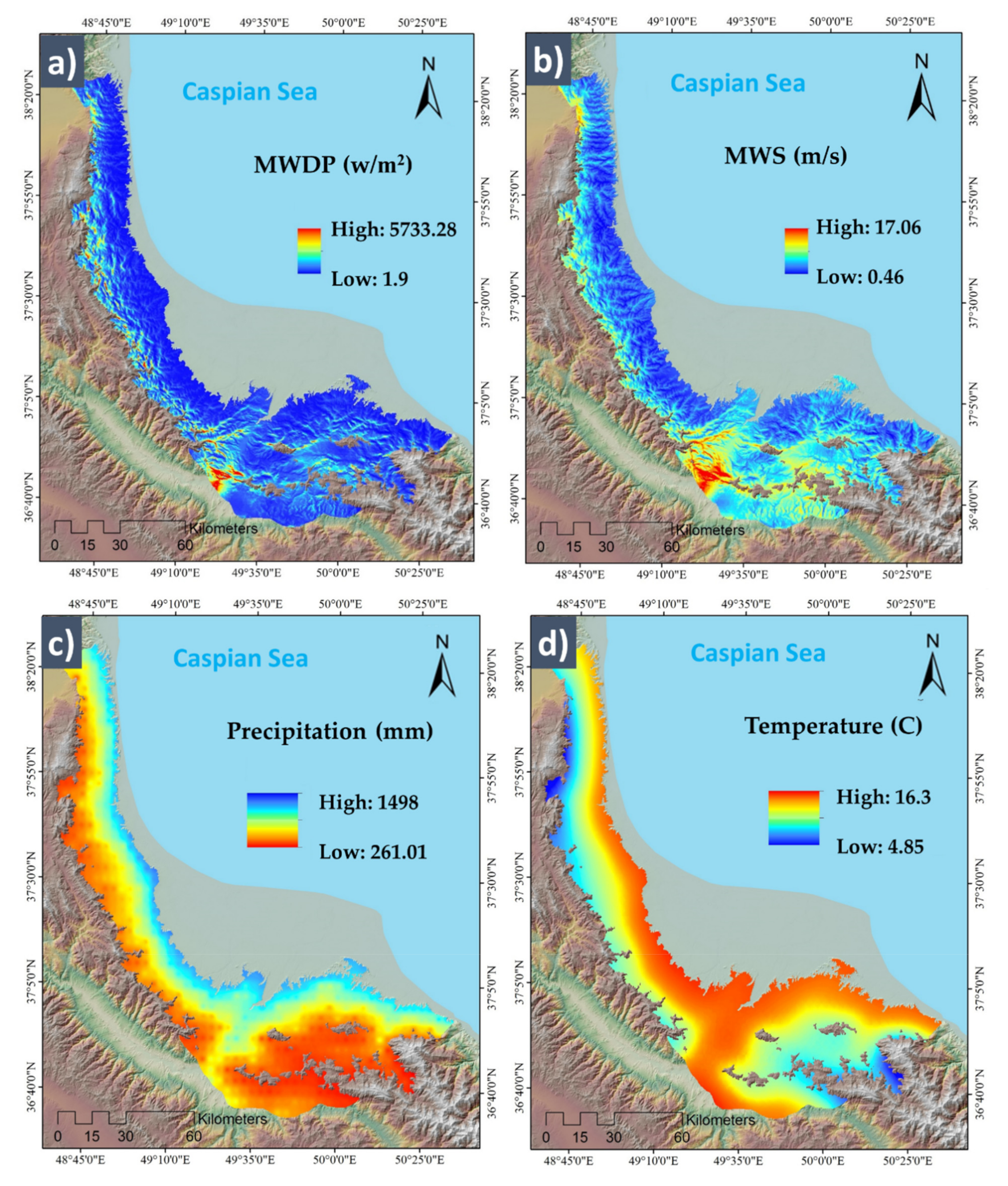
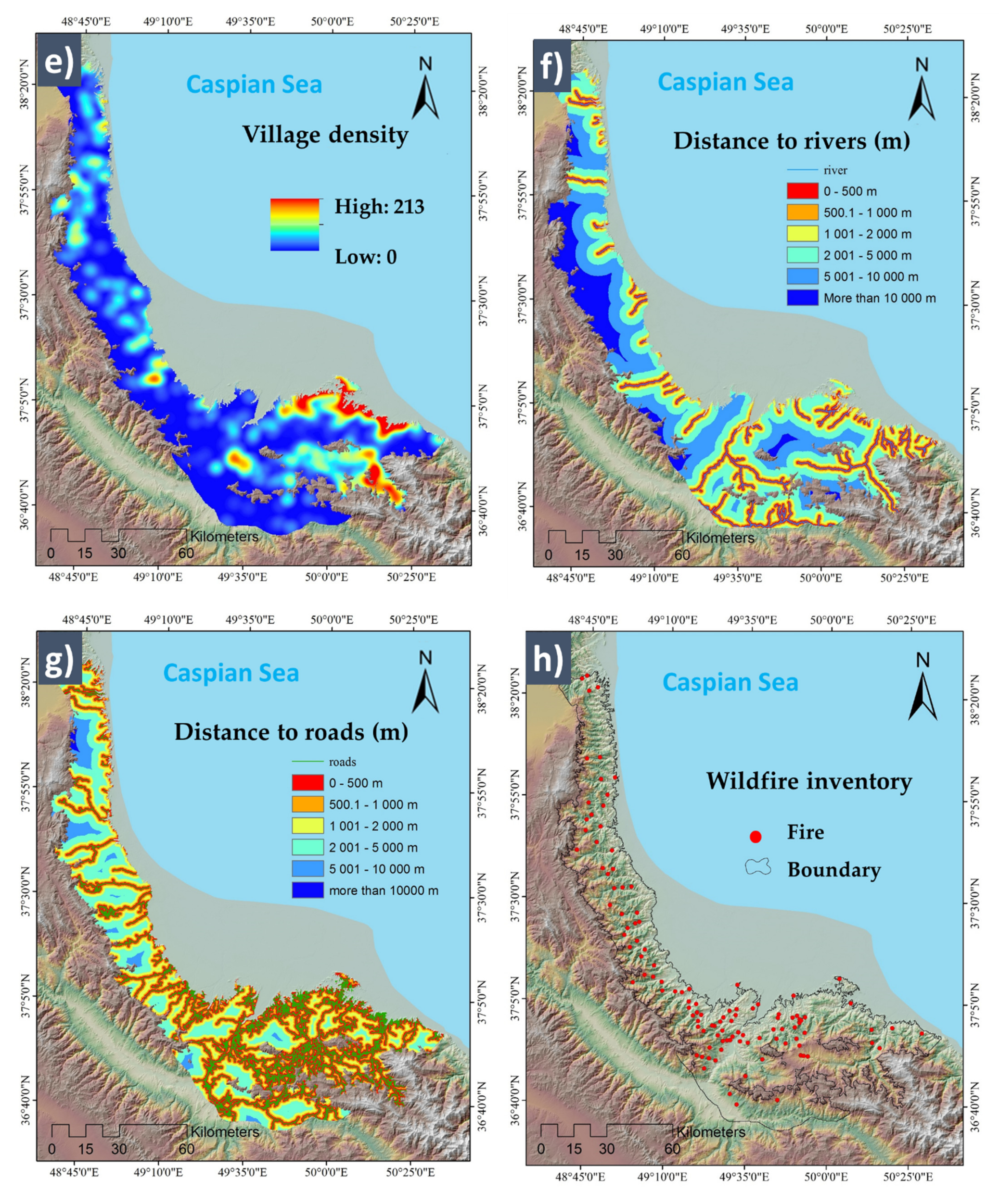
Conditioning Factors with Different Spatial Resolutions
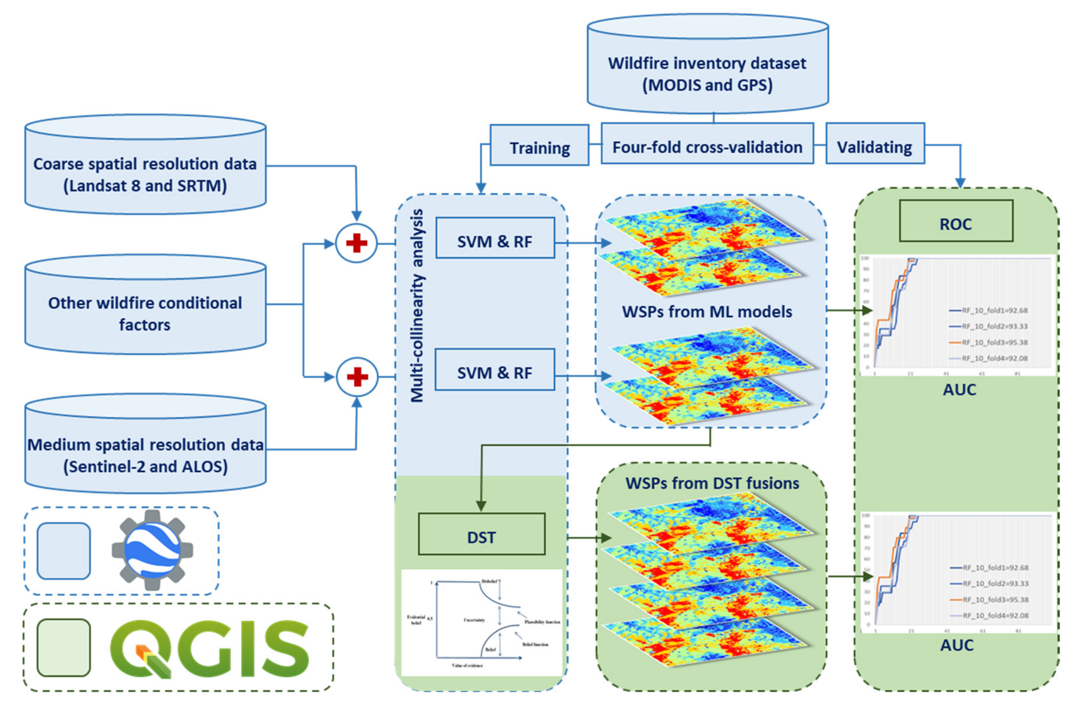
4. Methodology
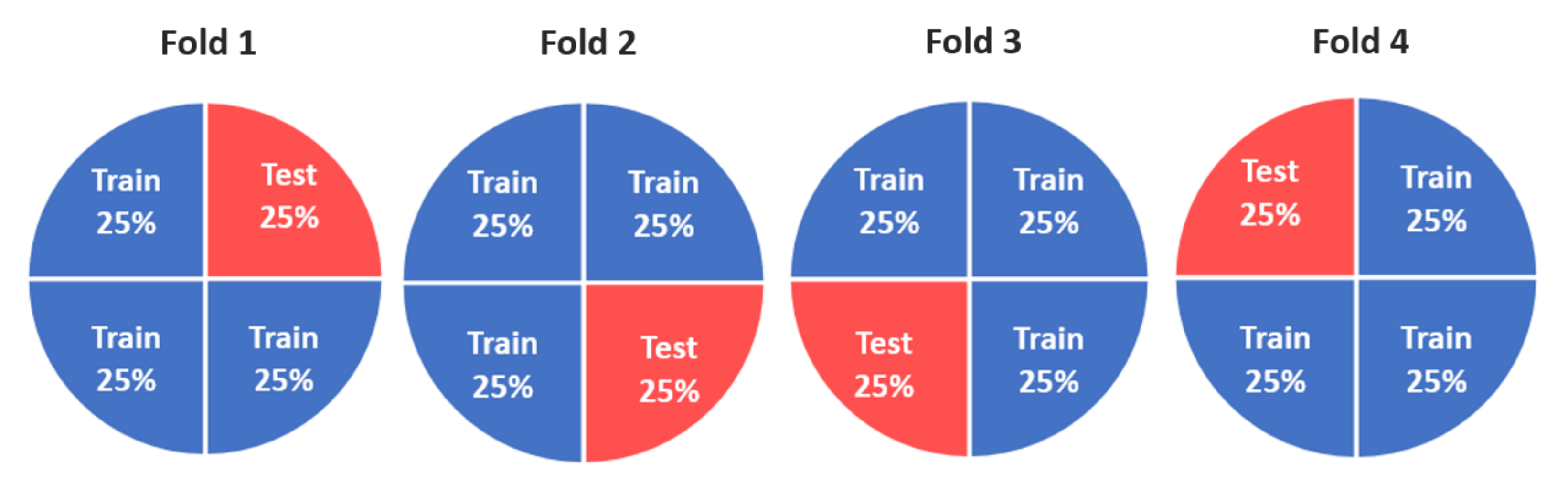
4.1. Training and Testing Dataset Organization
4.2. Factor Analysis
4.3. Google Earth Engine (GEE) Platform
4.4. Support Vector Machines (SVM)
4.5. Random Forest (RF)
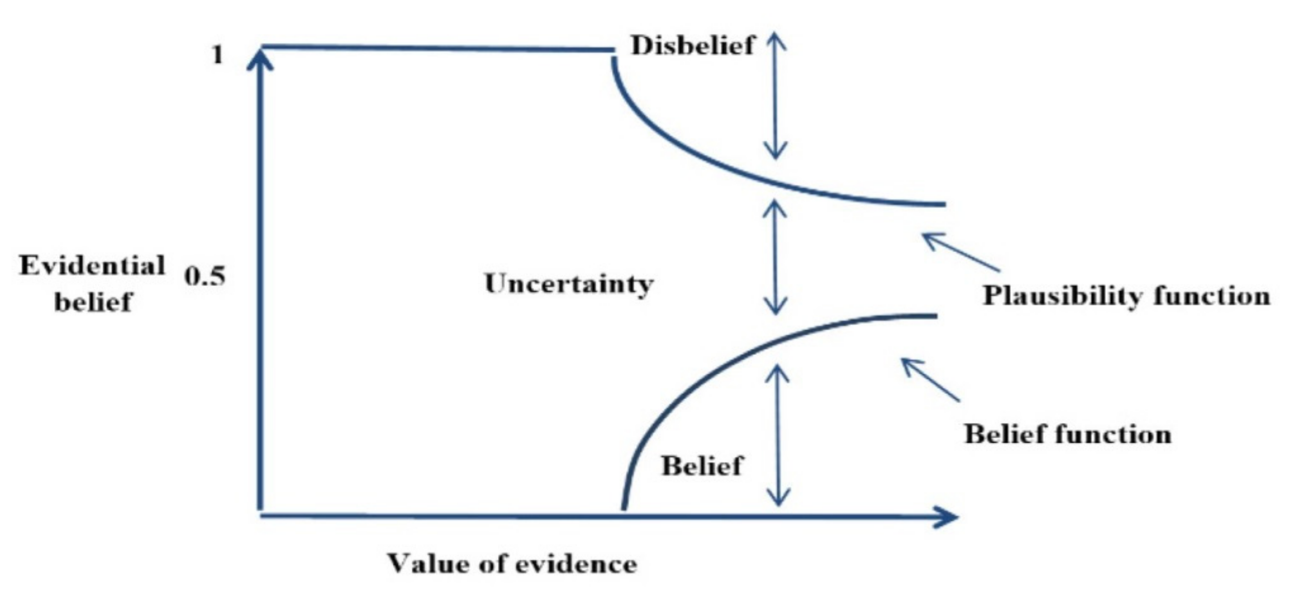
4.6. Dempster–Shafer Theory (DST)
5. Results
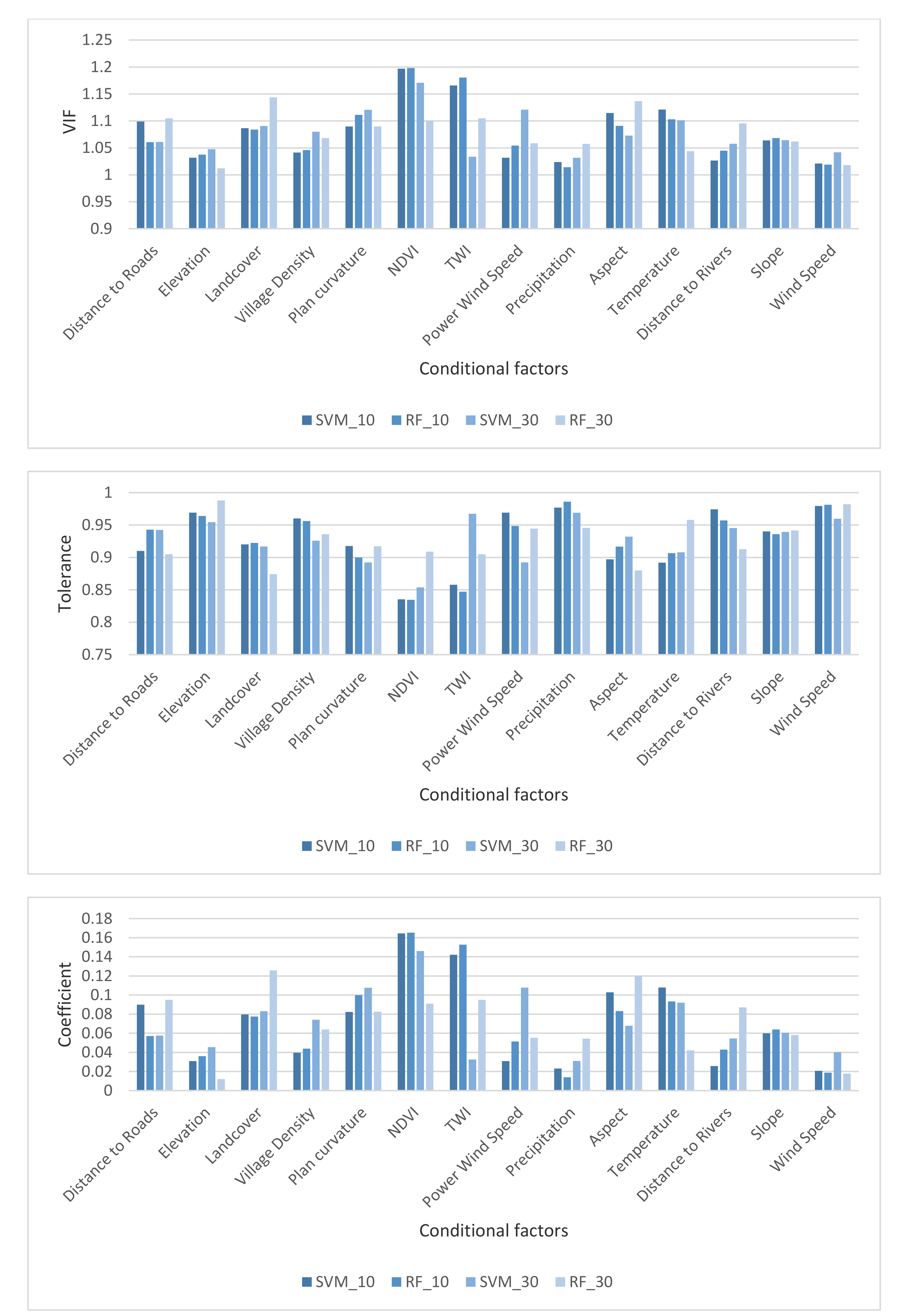
5.1. Multi-Collinearity Analysis among Conditional Factors
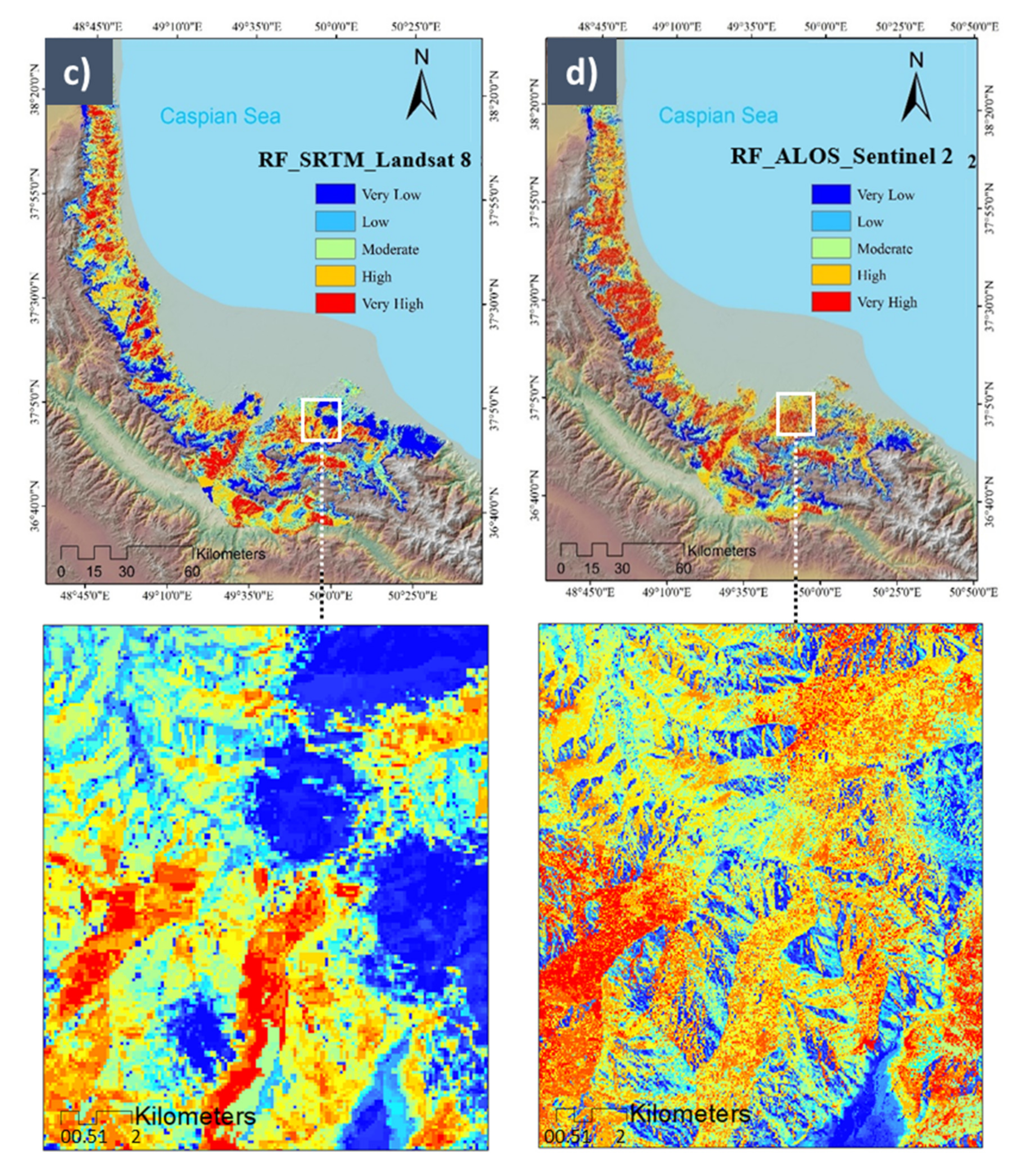
5.2. Wildfire Susceptibility Prediction (WSP) Maps Using Machine Learning (ML) Models
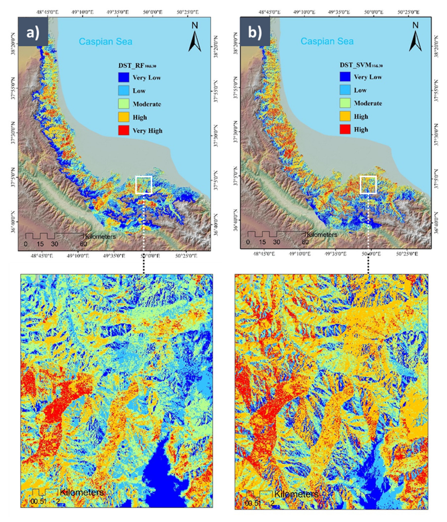
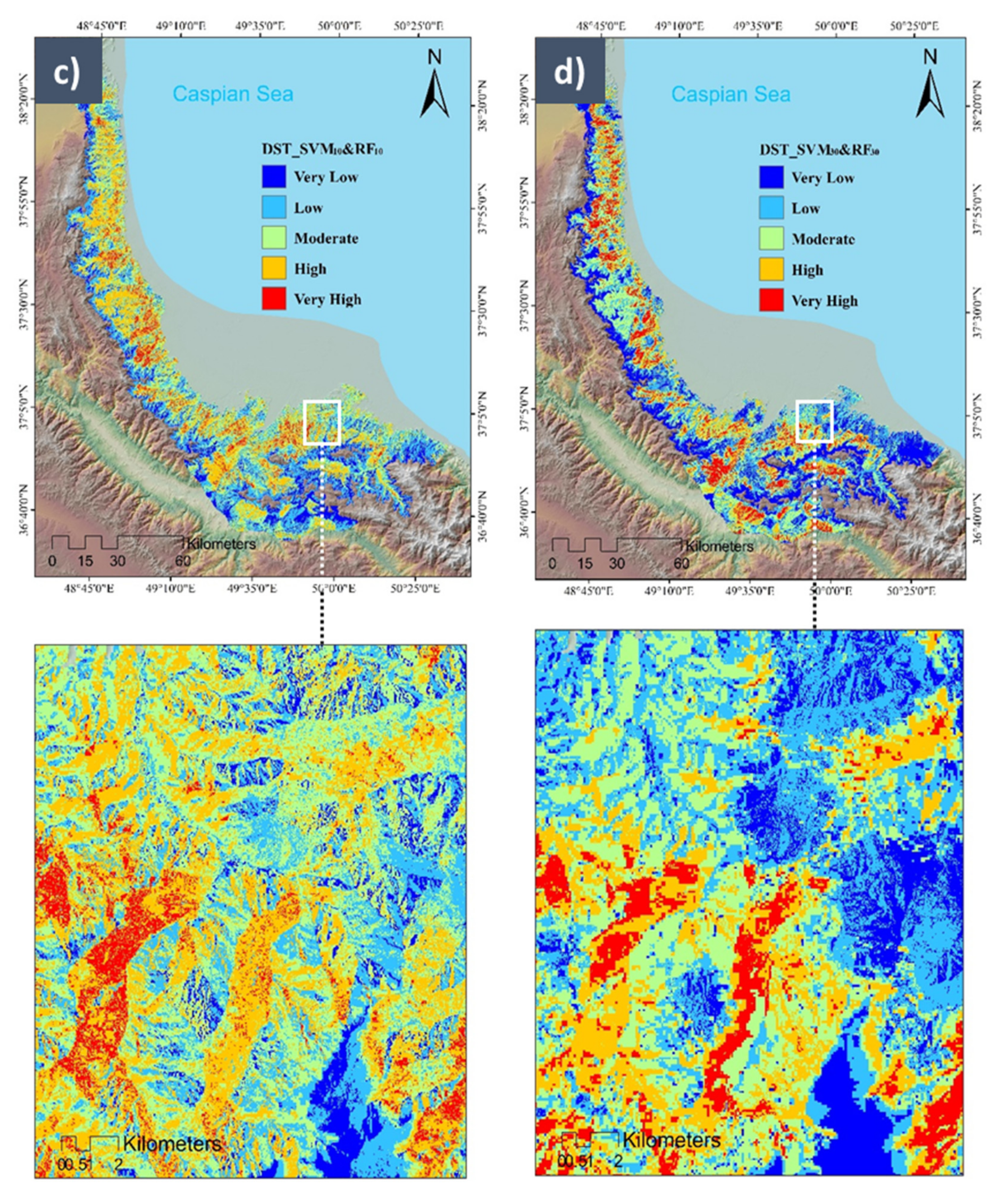
5.3. Dempster–Shafer Theory (DST) Optimization
5.4. Cross-Validation (CV)
6. Discussion
7. Conclusions
Author Contributions
Funding
Institutional Review Board Statement
Informed Consent Statement
Data Availability Statement
Acknowledgments
Conflicts of Interest
Abbreviations
| advanced spaceborne thermal emission and reflection radiometer | (ASTER) |
| advanced land observing satellite/phased array L-band synthetic aperture radar | (ALOS/PALSAR) |
| analytical hierarchical process | (AHP) |
| analytical network process | (ANP) |
| area under the curve | (AUC) |
| climate hazards group infrared precipitation with station data | (CHIRPS) |
| cross-validation | (CV) |
| Dempster–Shafer theory | (DST) |
| digital elevation model | (DEM) |
| European Space Agency | (ESA) |
| federal aviation administration | (FAA) |
| Google Earth Engine | (GEE) |
| geographic information system | (GIS) |
| global positioning system | (GPS) |
| machine learning | (ML) |
| mean wind speed | (MWS) |
| mean wind power density | (MWPD) |
| moderate resolution imaging spectroradiometer | (MODIS) |
| multi-criteria decision analysis | (MCDA) |
| National Aeronautics and Space Administration | (NASA) |
| National Oceanic and Atmospheric Administration National Weather Service | (NOAA-NWS) |
| Next-Generation Radar | (NEXRAD) |
| normalized difference vegetation index | (NDVI) |
| random forest | (RF) |
| receiver operating characteristic | (ROC) |
| remote sensing | (RS) |
| shuttle radar topography mission | (SRTM) |
| support vector machines | (SVM) |
| topographic wetness index | (TWI) |
| United States Geological Survey | (USGS) |
| US Air Force | (USAF) |
| variance inflation factor | (VIF) |
| wildfire susceptibility prediction | (WSP) |
References
- Ghorbanzadeh, O.; Blaschke, T.; Gholamnia, K.; Aryal, J. Forest fire susceptibility and risk mapping using social/infrastructural vulnerability and environmental variables. Fire 2019, 2, 50. [Google Scholar] [CrossRef] [Green Version]
- Moayedi, H.; Mehrabi, M.; Bui, D.T.; Pradhan, B.; Foong, L.K. Fuzzy-metaheuristic ensembles for spatial assessment of forest fire susceptibility. J. Environ. Manag. 2020, 260, 109867. [Google Scholar] [CrossRef] [PubMed]
- MacDicken, K.G. Global Forest Resources Assessment 2015: What, why and how? For. Ecol. Manag. 2015, 352, 3–8. [Google Scholar] [CrossRef] [Green Version]
- Sayad, Y.O.; Mousannif, H.; Al Moatassime, H. Predictive modeling of wildfires: A new dataset and machine learning approach. Fire Saf. J. 2019, 104, 130–146. [Google Scholar] [CrossRef]
- Hantson, S.; Pueyo, S.; Chuvieco, E. Global fire size distribution is driven by human impact and climate. Glob. Ecol. Biogeogr. 2015, 24, 77–86. [Google Scholar] [CrossRef]
- Tymstra, C.; Stocks, B.J.; Cai, X.; Flannigan, M.D. Wildfire management in Canada: Review, challenges and opportunities. Prog. Disaster Sci. 2020, 5, 100045. [Google Scholar] [CrossRef]
- Schlögel, R.; Marchesini, I.; Alvioli, M.; Reichenbach, P.; Rossi, M.; Malet, J.-P. Optimizing landslide susceptibility zonation: Effects of DEM spatial resolution and slope unit delineation on logistic regression models. Geomorphology 2018, 301, 10–20. [Google Scholar] [CrossRef]
- Tian, Y.; XiaO, C.; Liu, Y.; Wu, L. Effects of raster resolution on landslide susceptibility mapping: A case study of Shenzhen. Sci. China Ser. E Technol. Sci. 2008, 51, 188–198. [Google Scholar] [CrossRef]
- Avand, M.; Kuriqi, A.; Khazaei, M.; Ghorbanzadeh, O. DEM resolution effects on machine learning performance for flood probability mapping. J. Hydro-Environ. Res. 2022, 40, 1–16. [Google Scholar] [CrossRef]
- Eskandari, S.; Miesel, J.R. Comparison of the fuzzy AHP method, the spatial correlation method, and the Dong model to predict the fire high-risk areas in Hyrcanian forests of Iran. Geomat. Nat. Hazards Risk 2017, 8, 933–949. [Google Scholar] [CrossRef] [Green Version]
- Nami, M.; Jaafari, A.; Fallah, M.; Nabiuni, S. Spatial prediction of wildfire probability in the Hyrcanian ecoregion using evidential belief function model and GIS. Int. J. Environ. Sci. Technol. 2018, 15, 373–384. [Google Scholar] [CrossRef]
- Eskandari, S.; Pourghasemi, H.R.; Tiefenbacher, J.P. Fire-susceptibility mapping in the natural areas of Iran using new and ensemble data-mining models. Environ. Sci. Pollut. Res. 2021, 28, 47395–47406. [Google Scholar] [CrossRef] [PubMed]
- Jaafari, A.; Zenner, E.K.; Panahi, M.; Shahabi, H. Hybrid artificial intelligence models based on a neuro-fuzzy system and metaheuristic optimization algorithms for spatial prediction of wildfire probability. Agric. For. Meteorol. 2019, 266, 198–207. [Google Scholar] [CrossRef]
- Kalantar, B.; Ueda, N.; Idrees, M.O.; Janizadeh, S.; Ahmadi, K.; Shabani, F. Forest fire susceptibility prediction based on machine learning models with resampling algorithms on remote sensing data. Remote Sens. 2020, 12, 3682. [Google Scholar] [CrossRef]
- Naderpour, M.; Rizeei, H.M.; Ramezani, F. Forest Fire Risk Prediction: A Spatial Deep Neural Network-Based Framework. Remote Sens. 2021, 13, 2513. [Google Scholar] [CrossRef]
- Kim, S.; Lim, C.-H.; Kim, G.; Lee, J.; Geiger, T.; Rahmati, O.; Son, Y.; Lee, W.-K. Multi-temporal analysis of forest fire probability using socio-economic and environmental variables. Remote Sens. 2019, 11, 86. [Google Scholar] [CrossRef] [Green Version]
- Gholamnia, K.; Gudiyangada Nachappa, T.; Ghorbanzadeh, O.; Blaschke, T. Comparisons of Diverse Machine Learning Approaches for Wildfire Susceptibility Mapping. Symmetry 2020, 12, 604. [Google Scholar] [CrossRef] [Green Version]
- Khosravi, K.; Panahi, M.; Bui, D.T. Spatial prediction of groundwater spring potential mapping based on an adaptive neuro-fuzzy inference system and metaheuristic optimization. Hydrol. Earth Syst. Sci. 2018, 22, 4771–4792. [Google Scholar] [CrossRef] [Green Version]
- Mohammadi, A.; Karimzadeh, S.; Jalal, S.J.; Kamran, K.V.; Shahabi, H.; Homayouni, S.; Al-Ansari, N. A Multi-Sensor Comparative Analysis on the Suitability of Generated DEM from Sentinel-1 SAR Interferometry Using Statistical and Hydrological Models. Sensors 2020, 20, 7214. [Google Scholar] [CrossRef]
- Chen, Z.; Ye, F.; Fu, W.; Ke, Y.; Hong, H. The influence of DEM spatial resolution on landslide susceptibility mapping in the Baxie River basin, NW China. Nat. Hazards 2020, 101, 853–877. [Google Scholar] [CrossRef]
- Meena, S.R.; Gudiyangada Nachappa, T. Impact of Spatial Resolution of Digital Elevation Model on Landslide Susceptibility Mapping: A case Study in Kullu Valley, Himalayas. Geosciences 2019, 9, 360. [Google Scholar] [CrossRef] [Green Version]
- González, C.; Castillo, M.; García-Chevesich, P.; Barrios, J. Dempster-Shafer theory of evidence: A new approach to spatially model wildfire risk potential in central Chile. Sci. Total Environ. 2018, 613, 1024–1030. [Google Scholar] [CrossRef] [PubMed]
- Ghorbanzadeh, O.; Feizizadeh, B.; Blaschke, T. Multi-criteria risk evaluation by integrating an analytical network process approach into GIS-based sensitivity and uncertainty analyses. Geomat. Nat. Hazards Risk 2018, 9, 127–151. [Google Scholar] [CrossRef] [Green Version]
- Mezaal, M.; Pradhan, B.; Rizeei, H. Improving Landslide Detection from Airborne Laser Scanning Data Using Optimized Dempster–Shafer. Remote Sens. 2018, 10, 1029. [Google Scholar] [CrossRef] [Green Version]
- Nachappa, T.G.; Piralilou, S.T.; Gholamnia, K.; Ghorbanzadeh, O.; Rahmati, O.; Blaschke, T. Flood susceptibility mapping with machine learning, multi-criteria decision analysis and ensemble using Dempster Shafer Theory. J. Hydrol. 2020, 590, 125275. [Google Scholar] [CrossRef]
- Tehrany, M.S.; Kumar, L. The application of a Dempster–Shafer-based evidential belief function in flood susceptibility mapping and comparison with frequency ratio and logistic regression methods. Environ. Earth Sci. 2018, 77, 490. [Google Scholar] [CrossRef]
- Zarekar, A.; Zamani, B.K.; Ghorbani, S.; Moalla, M.A.; Jafari, H. Mapping spatial distribution of forest fire using MCDM and GIS (case study: Three forest zones in Guilan Province). Iran. J. For. Poplar Res. 2013, 21, 218–230. [Google Scholar]
- Arnone, E.; Francipane, A.; Scarbaci, A.; Puglisi, C.; Noto, L.V. Effect of raster resolution and polygon-conversion algorithm on landslide susceptibility mapping. Environ. Model. Softw. 2016, 84, 467–481. [Google Scholar] [CrossRef]
- Rahmati, O.; Pourghasemi, H.R.; Zeinivand, H. Flood susceptibility mapping using frequency ratio and weights-of-evidence models in the Golastan Province, Iran. Geocarto Int. 2015, 31, 42–70. [Google Scholar] [CrossRef]
- Eskandari, S.; Khoshnevis, M. Evaluating and mapping the fire risk in the forests and rangelands of Sirachal using fuzzy analytic hierarchy process and GIS. J. For. Res. Dev. 2020, 6, 219–245. [Google Scholar]
- Ljubomir, G.; Pamučar, D.; Drobnjak, S.; Pourghasemi, H.R. Modeling the Spatial Variability of Forest Fire Susceptibility Using Geographical Information Systems and the Analytical Hierarchy Process. In Spatial Modeling in GIS and R for Earth and Environmental Sciences; Elsevier: Amsterdam, The Netherlands, 2019; pp. 337–369. [Google Scholar] [CrossRef]
- Jaafari, A.; Pourghasemi, H.R. Factors Influencing Regional-Scale Wildfire Probability in Iran. In Spatial Modeling in GIS and R for Earth and Environmental Sciences; Elsevier: Amsterdam, The Netherlands, 2019; pp. 607–619. [Google Scholar] [CrossRef]
- Chen, H.X.; Zhang, S.; Peng, M.; Zhang, L.M. A physically-based multi-hazard risk assessment platform for regional rainfall-induced slope failures and debris flows. Eng. Geol. 2016, 203, 15–29. [Google Scholar] [CrossRef]
- Pourtaghi, Z.S.; Pourghasemi, H.R.; Rossi, M. Forest fire susceptibility mapping in the Minudasht forests, Golestan province, Iran. Environ. Earth Sci. 2015, 73, 1515–1533. [Google Scholar] [CrossRef]
- Molina, J.R.; Gonzalez-Caban, A.; Rodriguez, Y.S.F. Wildfires impact on the economic susceptibility of recreation activities: Application in a Mediterranean protected area. J. Environ. Manag. 2019, 245, 454–463. [Google Scholar] [CrossRef] [PubMed]
- Tien Bui, D.; Le, K.-T.; Nguyen, V.; Le, H.; Revhaug, I. Tropical Forest Fire Susceptibility Mapping at the Cat Ba National Park Area, Hai Phong City, Vietnam, Using GIS-Based Kernel Logistic Regression. Remote Sens. 2016, 8, 347. [Google Scholar] [CrossRef] [Green Version]
- Ghorbanzadeh, O.; Valizadeh Kamran, K.; Blaschke, T.; Aryal, J.; Naboureh, A.; Einali, J.; Bian, J. Spatial Prediction of Wildfire Susceptibility Using Field Survey GPS Data and Machine Learning Approaches. Fire 2019, 2, 43. [Google Scholar] [CrossRef] [Green Version]
- Gudiyangada Nachappa, T.; Tavakkoli Piralilou, S.; Ghorbanzadeh, O.; Shahabi, H.; Blaschke, T. Landslide Susceptibility Mapping for Austria Using Geons and Optimization with the Dempster-Shafer Theory. Appl. Sci. 2019, 9, 5393. [Google Scholar] [CrossRef] [Green Version]
- Verde, J.; Zêzere, J. Assessment and validation of wildfire susceptibility and hazard in Portugal. Nat. Hazards Earth Syst. Sci. 2010, 10, 485–497. [Google Scholar] [CrossRef]
- Shakesby, R.A. Post-wildfire soil erosion in the Mediterranean: Review and future research directions. Earth-Sci. Rev. 2011, 105, 71–100. [Google Scholar] [CrossRef]
- Ghorbanzadeh, O.; Rostamzadeh, H.; Blaschke, T.; Gholaminia, K.; Aryal, J. A new GIS-based data mining technique using an adaptive neuro-fuzzy inference system (ANFIS) and k-fold cross-validation approach for land subsidence susceptibility mapping. Nat. Hazards 2018, 94, 497–517. [Google Scholar] [CrossRef] [Green Version]
- Costache, R.; Arabameri, A.; Elkhrachy, I.; Ghorbanzadeh, O.; Pham, Q.B. Detection of areas prone to flood risk using state-of-the-art machine learning models. Geomat. Nat. Hazards Risk 2021, 12, 1488–1507. [Google Scholar] [CrossRef]
- Hong, H.; Pradhan, B.; Sameen, M.I.; Chen, W.; Xu, C. Spatial prediction of rotational landslide using geographically weighted regression, logistic regression, and support vector machine models in Xing Guo area (China). Geomat. Nat. Hazards Risk 2017, 8, 1997–2022. [Google Scholar] [CrossRef] [Green Version]
- Cossu, R.; Petitdidier, M.; Linford, J.; Badoux, V.; Fusco, L.; Gotab, B.; Hluchy, L.; Lecca, G.; Murgia, F.; Plevier, C.; et al. A roadmap for a dedicated Earth Science Grid platform. Earth Sci. Inform. 2010, 3, 135–148. [Google Scholar] [CrossRef] [Green Version]
- Loveland, T.R.; Dwyer, J.L. Landsat: Building a strong future. Remote Sens. Environ. 2012, 122, 22–29. [Google Scholar] [CrossRef]
- Sudmanns, M.; Tiede, D.; Lang, S.; Bergstedt, H.; Trost, G.; Augustin, H.; Baraldi, A.; Blaschke, T. Big Earth data: Disruptive changes in Earth observation data management and analysis? Int. J. Digit. Earth 2019, 13, 832–850. [Google Scholar] [CrossRef] [PubMed]
- Gorelick, N.; Hancher, M.; Dixon, M.; Ilyushchenko, S.; Thau, D.; Moore, R. Google Earth Engine: Planetary-scale geospatial analysis for everyone. Remote Sens. Environ. 2017, 202, 18–27. [Google Scholar] [CrossRef]
- GoogleEarthEngine. Available online: https://earthengine.google.com/#intro (accessed on 17 May 2020).
- Vapnik, V. The Nature of Statistical Learning Theory; Springer Science & Business Media: Berlin/Heidelberg, Germany, 2013. [Google Scholar]
- Kavzoglu, T.; Sahin, E.K.; Colkesen, I. Landslide susceptibility mapping using GIS-based multi-criteria decision analysis, support vector machines, and logistic regression. Landslides 2013, 11, 425–439. [Google Scholar] [CrossRef]
- Ghamisi, P.; Plaza, J.; Chen, Y.; Li, J.; Plaza, A.J. Advanced spectral classifiers for hyperspectral images: A review. IEEE Geosci. Remote Sens. Mag. 2017, 5, 8–32. [Google Scholar] [CrossRef] [Green Version]
- Mohammadi, A.; Shahabi, H.; Bin Ahmad, B. Land-Cover Change Detection in a Part of Cameron Highlands, Malaysia Using ETM+ Satellite Imagery and Support Vector Machine (SVM) Algorithm. EnvironmentAsia 2019, 12, 145–154. [Google Scholar]
- Tehrany, M.S.; Pradhan, B.; Mansor, S.; Ahmad, N. Flood susceptibility assessment using GIS-based support vector machine model with different kernel types. Catena 2015, 125, 91–101. [Google Scholar] [CrossRef]
- Bui, D.T.; Tuan, T.A.; Klempe, H.; Pradhan, B.; Revhaug, I. Spatial prediction models for shallow landslide hazards: A comparative assessment of the efficacy of support vector machines, artificial neural networks, kernel logistic regression, and logistic model tree. Landslides 2016, 13, 361–378. [Google Scholar]
- Ho, T.K. Random decision forests. In Proceedings of the 3rd International Conference on Document Analysis and Recognition, Montreal, QC, Canada, 14–16 August 1995; pp. 278–282. [Google Scholar]
- Breiman, L. Random forests. Mach. Learn. 2001, 45, 5–32. [Google Scholar] [CrossRef] [Green Version]
- Pourghasemi, H.R.; Rahmati, O. Prediction of the landslide susceptibility: Which algorithm, which precision? Catena 2018, 162, 177–192. [Google Scholar] [CrossRef]
- Xu, R.; Lin, H.; Lü, Y.; Luo, Y.; Ren, Y.; Comber, A. A Modified Change Vector Approach for Quantifying Land Cover Change. Remote Sens. 2018, 10, 1578. [Google Scholar] [CrossRef] [Green Version]
- Ghorbanzadeh, O.; Blaschke, T.; Gholamnia, K.; Meena, S.R.; Tiede, D.; Aryal, J. Evaluation of Different Machine Learning Methods and Deep-Learning Convolutional Neural Networks for Landslide Detection. Remote Sens. 2019, 11, 196. [Google Scholar] [CrossRef] [Green Version]
- Valdez, M.C.; Chang, K.-T.; Chen, C.-F.; Chiang, S.-H.; Santos, J.L. Modelling the spatial variability of wildfire susceptibility in Honduras using remote sensing and geographical information systems. Geomat. Nat. Hazards Risk 2017, 8, 876–892. [Google Scholar] [CrossRef] [Green Version]
- Feizizadeh, B. A Novel Approach of Fuzzy Dempster–Shafer Theory for Spatial Uncertainty Analysis and Accuracy Assessment of Object-Based Image Classification. IEEE Geosci. Remote Sens. Lett. 2018, 15, 18–22. [Google Scholar] [CrossRef]
- Fei, L.; Xia, J.; Feng, Y.; Liu, L. A novel method to determine basic probability assignment in Dempster–Shafer theory and its application in multi-sensor information fusion. Int. J. Distrib. Sens. Netw. 2019, 15, 1550147719865876. [Google Scholar]
- Ghorbanzadeh, O.; Meena, S.R.; Abadi, H.S.S.; Piralilou, S.T.; Zhiyong, L.; Blaschke, T. Landslide Mapping Using Two Main Deep-Learning Convolution Neural Network (CNN) Streams Combined by the Dempster—Shafer (DS) model. IEEE J. Sel. Top. Appl. Earth Obs. Remote Sens. 2020, 14, 452–463. [Google Scholar] [CrossRef]
- Shahabi, H.; Jarihani, B.; Tavakkoli Piralilou, S.; Chittleborough, D.; Avand, M.; Ghorbanzadeh, O. A Semi-Automated Object-Based Gully Networks Detection Using Different Machine Learning Models: A Case Study of Bowen Catchment, Queensland, Australia. Sensors 2019, 19, 4893. [Google Scholar] [CrossRef] [Green Version]
- Shafer, G. A mathematical theory of evidence; Princeton University Press: Princeton, NJ, USA, 1976. [Google Scholar]
- Rahmati, O.; Melesse, A.M. Application of Dempster–Shafer theory, spatial analysis and remote sensing for groundwater potentiality and nitrate pollution analysis in the semi-arid region of Khuzestan, Iran. Sci. Total Environ. 2016, 568, 1110–1123. [Google Scholar] [CrossRef]
- Schneider, L.C.; Pontius, R.G., Jr. Modeling land-use change in the Ipswich watershed, Massachusetts, USA. Agric. Ecosyst. Environ. 2001, 85, 83–94. [Google Scholar] [CrossRef]


| Dataset | Resolution |
|---|---|
| Landsat-8 | 30 m |
| Sentinel-2 | 10 m |
| SRTM | 30 m |
| ALOS PALSAR | 12.5 m |
| Conditioning Factor | Source | Importance | References |
|---|---|---|---|
| Elevation | ALOS SRTM | The elevation is an essential feature of regional climate variations. The higher moisture in highlands prevents severe wildfires. | [1,32] |
| Slope | ALOS SRTM | This factor controls biodiversity and vegetation distribution. Additionally, fire fronts are faster on upward slopes. | [31,33] |
| Aspect | ALOS SRTM | Wildfire is distributed faster on east-facing slopes that receive more incoming solar radiation in mountainous areas. | [1,14,34] |
| Plan curvature | ALOS SRTM | This factor illustrates concavity or convexity of the topography, which is beneficial for assessing soil water content and distribution of vegetation. | [14] |
| TWI | ALOS SRTM | This factor defines the aspect of steady-state soil wetness and is calculated as TWI = ln(α/tanβ) where α is the cumulative upslope drainage area for a given pixel, whereas tanβ is the slope angle at that pixel. | [12] |
| Landcover | Sentinel-2 Landsat 8 | Different landcover patterns have different impacts on wildfire distribution and risk. It is related to the interaction between the cover type and human activity. | [17,35,36] |
| NDVI | Sentinel-2 Landsat 8 | This index reflects the crown water content and the decrease of this index represents water stress, which provides more dry grass, brush, and trees (fuel) for wildfire, increasing its ignition probability and spread speed. | [12] |
| Distance to rivers | GIS data | Rivers are one of the entertaining human interests, and human activity directly relates to the wildfires. | [34,37] |
| Distance to roads | Open street map | This factor quantifies access to forest areas, anthropological movement, and human activities. | [16,38] |
| Temperature | Meteorological data | Radiant heat. | [34,39] |
| Precipitation | Meteorological data | Vegetation pattern and existing moisture that influence the speed of fire distribution. | [12,36] |
| Village density | Open street map | This index is used as a proxy for the amount of human activity. | [31,34] |
| MWPD | Wind global atlas | The mean wind power density (MWPD) measures the wind resource, which is also related to moistness content and oxygen. | [35] |
| MWS | Wind global atlas | The mean wind speed (MWS) is related to wildfires as the wind usually spreads the fire in the wind direction and makes it faster and more dangerous. | [13,40] |
| AUC Values | Linguistic Explanation |
|---|---|
| 1–0.90 | Excellent |
| 0.90–0.80 | Good |
| 0.80–0.70 | Fair |
| 0.70–0.60 | Poor |
| 0.60–0.50 | Fail |
| Method | AUC Fold 1 | AUC Fold 2 | AUC Fold 3 | AUC Fold 4 | AUC CV |
|---|---|---|---|---|---|
| SVM10 | 92.59 | 91.44 | 95.98 | 90 | 92.5 |
| SVM30 | 91.6 | 91.67 | 95.77 | 89.58 | 92.15 |
| RF10 | 92.68 | 93.33 | 95.38 | 92.08 | 93.37 |
| RF30 | 89.08 | 89.58 | 94.78 | 94.59 | 91.89 |
| DST_ SVM10 & 30 | 92.88 | 92.4 | 96.26 | 91.06 | 93.15 |
| DST_ RF10 & 30 | 93.32 | 92.97 | 97.36 | 95.21 | 94.71 |
| DST_ SVM10 & RF10 | 93.12 | 94.51 | 97.55 | 93.13 | 94.57 |
| DST_ SVM30 & RF30 | 92.37 | 92.36 | 95.09 | 94.21 | 93.5 |
| Average of each fold | 92.2 | 92.3 | 96.02 | 92.49 | 93.23 |
| Method | Very low | Low | Moderate | High | Very high |
|---|---|---|---|---|---|
| SVM10 | 18.08 | 22.55 | 22.31 | 26.91 | 10.12 |
| SVM30 | 13.78 | 29.94 | 27.6 | 24.28 | 4.36 |
| RF10 | 28.6 | 20.31 | 21.05 | 18.8 | 11.22 |
| RF30 | 31.98 | 21.02 | 21.31 | 14.94 | 10.73 |
| DST_ SVM10 & 30 | 17.81 | 22.77 | 22.31 | 28.46 | 8.63 |
| DST_ RF10 & 30 | 23.9 | 26.37 | 24.01 | 19.8 | 5.89 |
| DST_ SVM10 & RF10 | 25.57 | 25.8 | 24.03 | 14.85 | 9.74 |
| DST_ SVM30 & RF30 | 20.96 | 23.22 | 27.14 | 20.06 | 8.5 |
Publisher’s Note: MDPI stays neutral with regard to jurisdictional claims in published maps and institutional affiliations. |
© 2022 by the authors. Licensee MDPI, Basel, Switzerland. This article is an open access article distributed under the terms and conditions of the Creative Commons Attribution (CC BY) license (https://creativecommons.org/licenses/by/4.0/).
Share and Cite
Tavakkoli Piralilou, S.; Einali, G.; Ghorbanzadeh, O.; Nachappa, T.G.; Gholamnia, K.; Blaschke, T.; Ghamisi, P. A Google Earth Engine Approach for Wildfire Susceptibility Prediction Fusion with Remote Sensing Data of Different Spatial Resolutions. Remote Sens. 2022, 14, 672. https://doi.org/10.3390/rs14030672
Tavakkoli Piralilou S, Einali G, Ghorbanzadeh O, Nachappa TG, Gholamnia K, Blaschke T, Ghamisi P. A Google Earth Engine Approach for Wildfire Susceptibility Prediction Fusion with Remote Sensing Data of Different Spatial Resolutions. Remote Sensing. 2022; 14(3):672. https://doi.org/10.3390/rs14030672
Chicago/Turabian StyleTavakkoli Piralilou, Sepideh, Golzar Einali, Omid Ghorbanzadeh, Thimmaiah Gudiyangada Nachappa, Khalil Gholamnia, Thomas Blaschke, and Pedram Ghamisi. 2022. "A Google Earth Engine Approach for Wildfire Susceptibility Prediction Fusion with Remote Sensing Data of Different Spatial Resolutions" Remote Sensing 14, no. 3: 672. https://doi.org/10.3390/rs14030672