
Mapping Outburst Floods Using a Collaborative Learning Method Based on Temporally Dense Optical and SAR Data: A Case Study with the Baige Landslide Dam on the Jinsha River, Tibet

 ,
,
Abstract
:1. Introduction
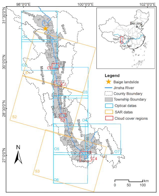
2. Study Area
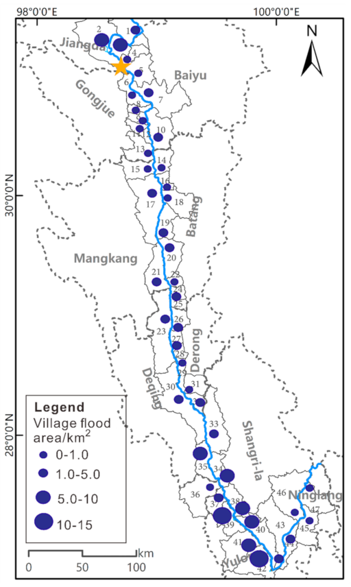
2.1. The Outburst Flood Resulting from Baige Landslide Dam Break on 3 November 2018
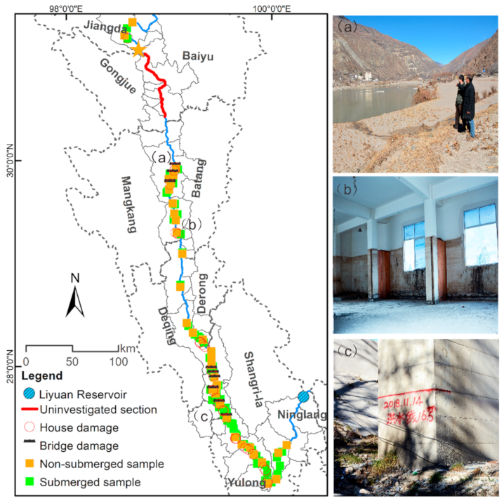
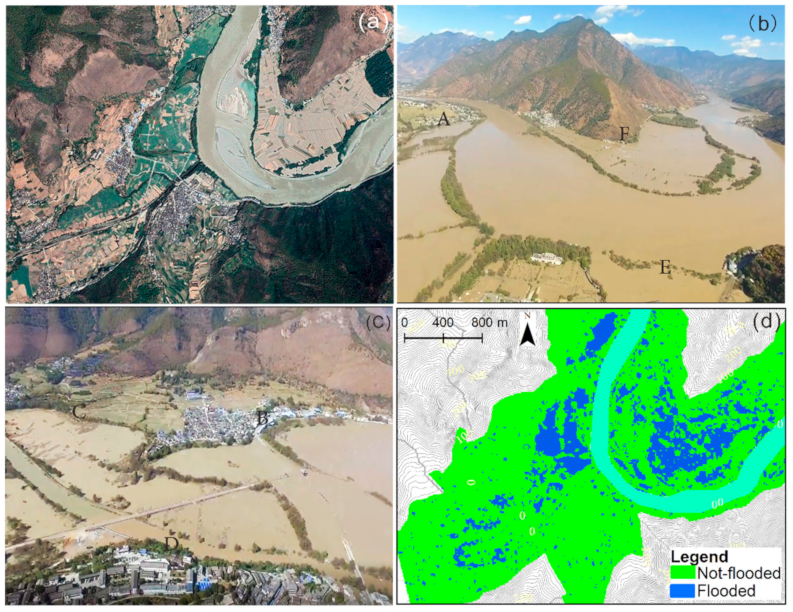
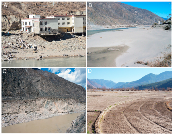
2.2. Field Investigation
3. Data
3.1. Sentinel-2 Dates
3.2. Sentinel-1 Dates
3.3. DEM Date and Height Difference
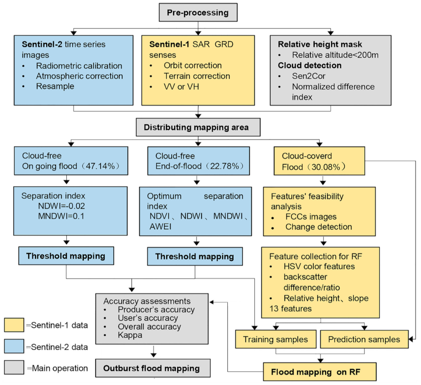
4. Methods
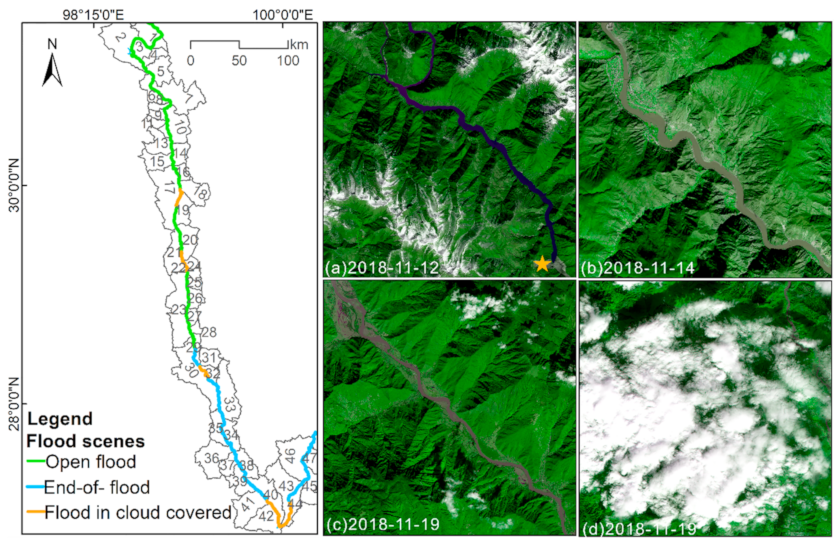
4.1. Flood Mapping Based on Sentinel-2 Optical Images in the Cloud-Free Area
4.1.1. Open Water Mapping (Barrier Lake and Ongoing Flood)
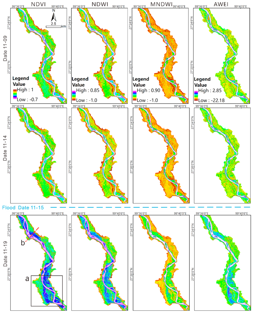
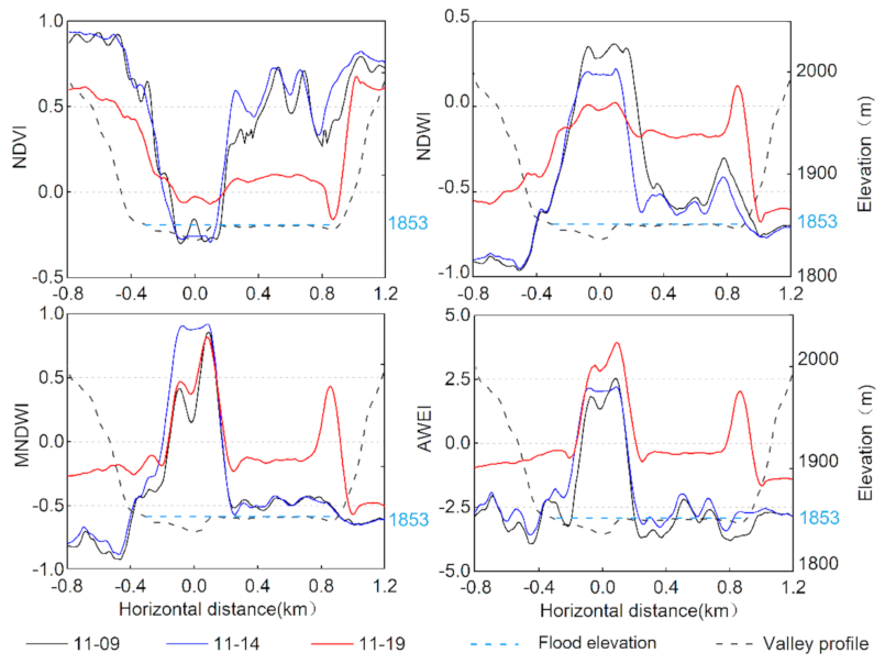
4.1.2. Optimal Spectral Index for End-of-Flood Mapping
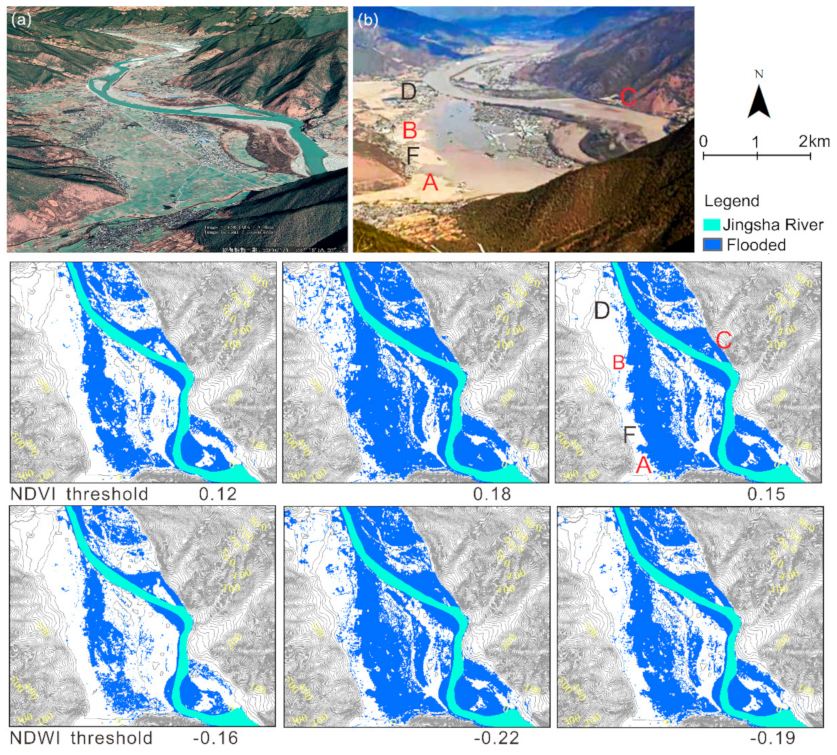
4.1.3. Optimal Threshold for End-of-Flood Mapping
4.2. Effective Flood Mapping Features Based on Sentinel-1 SAR Images
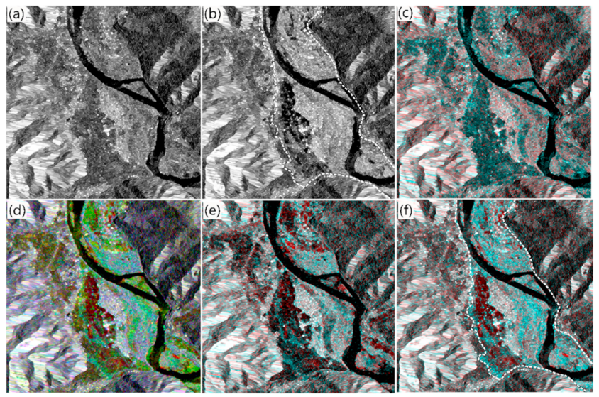
4.2.1. RGB False Color Composites Images
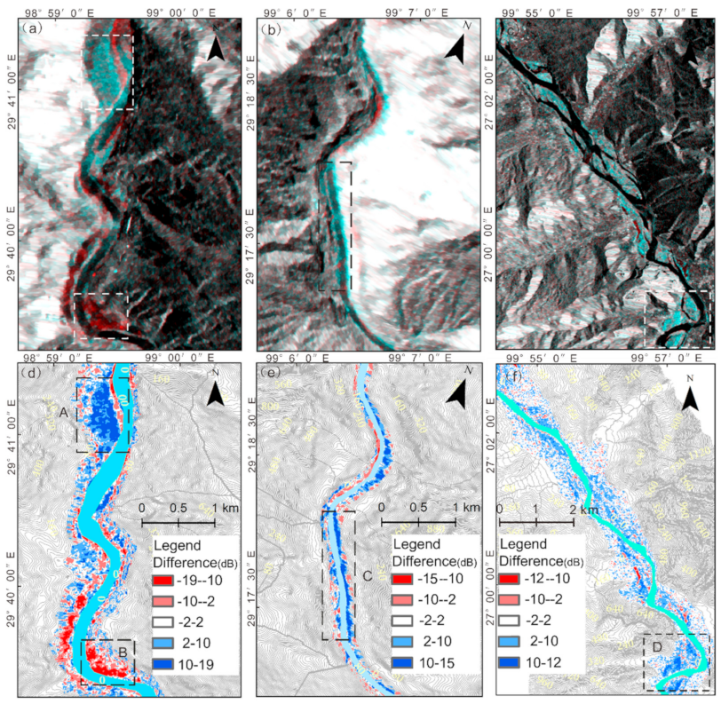
4.2.2. The Backscatter Difference on Sentinel-1 SAR Date
4.3. Flood Classification by RF Algorithm on Sentinel-1 Images in the Cloud-Covered Area
4.3.1. RF Algorithm
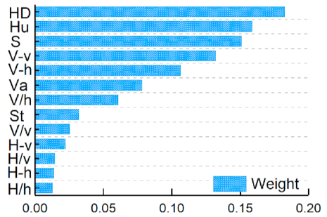
4.3.2. Feasible Features Combination
HSV Color Feature Extraction
Calculation of Backscatter Difference/Ratio Images
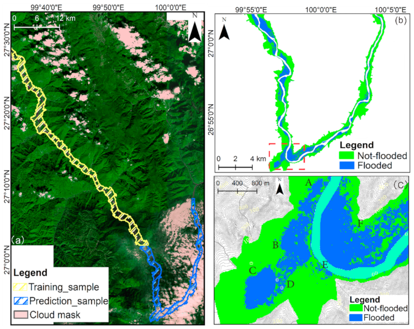
4.3.3. Training and Prediction Data
5. Results
5.1. Prediction Mapping of RF Algorithm on Sentinel-1 Images
5.2. Flood Mapping Accuracy
5.3. Flood Area Statistics
6. Discussion
6.1. The Relationship of Backscatter Differences and the Outburst Flood
6.2. Reliability of Flood Mapping Using a Collaborative Learning Method
7. Conclusions
Author Contributions
Funding
Data Availability Statement
Conflicts of Interest
Abbreviations
| Acronym | Description |
| AWEI | Automated water extraction index |
| CDAT | Change detection and thresholding |
| DEM | Digital elevation model |
| FCCs | RGB false color composites method |
| HSBA | Hierarchical split-based approach |
| HSV | Hue-saturation-value color space |
| IW | Interference wide mode |
| KI | Kittler and Illingworth |
| MNDWI | Modified normalised difference water index |
| NDVI | Normalized difference vegetation index |
| NDWI | Normalised difference water index |
| NIR | Near-infrared band |
| LiDAR | Light detection and ranging |
| OA | Overall accuracy |
| Otsu | Otsu adapting threshold |
| PA | Producer’s accuracy |
| RF | Random Forest algorithm |
| SAR | Synthetic Aperture Radar |
| SRTM | Shuttle Radar Topography Mission |
| SWIR | Shortwave infrared band |
| TCT | Tasseled Cap Transformation |
| UA | User’s accuracy |
| UAV | Unmanned Aerial Vehicle |
| VH | Polarization of vertical transmit-horizontal receive |
| VV | Polarization of vertical transmit-vertical receive |
References
- Baker, V.R. 9.26 Global Late Quaternary Fluvial Paleohydrology: With Special Emphasis on Paleofloods and Megafloods. Treatise Geomorphol. 2013, 511–527. [Google Scholar] [CrossRef]
- Fan, X.; Scaringi, G.; Korup, O.; West, A.J.; Van Westen, C.J.; Tanyas, H.; Hovius, N.; Hales, T.C.; Jibson, R.W.; Allstadt, K.E.; et al. Earthquake-Induced Chains of Geologic Hazards: Patterns, Mechanisms, and Impacts. Rev. Geophys. 2019, 57, 421–503. [Google Scholar] [CrossRef] [Green Version]
- Zhou, J.-W.; Cui, P.; Hao, M.-H. Comprehensive analyses of the initiation and entrainment processes of the 2000 Yigong catastrophic landslide in Tibet, China. Landslides 2015, 13, 39–54. [Google Scholar] [CrossRef]
- Zhong, Q.; Chen, S.; Wang, L.; Shan, Y. Back analysis of breaching process of Baige landslide dam. Landslides 2020, 17, 1681–1692. [Google Scholar] [CrossRef]
- Liu, W.; Carling, P.A.; Hu, K.; Wang, H.; Zhou, Z.; Zhou, L.; Liu, D.; Lai, Z.; Zhang, X. Outburst floods in China: A review. Earth Sci. Rev. 2019, 197, 102895. [Google Scholar] [CrossRef]
- Markert, K.N.; Markert, A.M.; Mayer, T.; Nauman, C.; Haag, A.; Poortinga, A.; Bhandari, B.; Thwal, N.S.; Kunlamai, T.; Chishtie, F.; et al. Comparing Sentinel-1 Surface Water Mapping Algorithms and Radiometric Terrain Correction Processing in Southeast Asia Utilizing Google Earth Engine. Remote Sens. 2020, 12, 2469. [Google Scholar] [CrossRef]
- Bhardwaj, A.; Singh, M.K.; Joshi, P.; Snehmani; Singh, S.; Sam, L.; Gupta, R.; Kumar, R. A lake detection algorithm (LDA) using Landsat 8 data: A comparative approach in glacial environment. Int. J. Appl. Earth Obs. Geoinf. 2015, 38, 150–163. [Google Scholar] [CrossRef]
- McFeeters, S.K. The use of the Normalized Difference Water Index (NDWI) in the delineation of open water features. Int. J. Remote Sens. 1996, 17, 1425–1432. [Google Scholar] [CrossRef]
- Xu, H. Modification of normalised difference water index (NDWI) to enhance open water features in remotely sensed imagery. Int. J. Remote Sens. 2006, 27, 3025–3033. [Google Scholar] [CrossRef]
- Sanyal, J.; Lu, X. Application of Remote Sensing in Flood Management with Special Reference to Monsoon Asia: A Review. Nat. Hazards 2004, 33, 283–301. [Google Scholar] [CrossRef]
- Feyisa, G.L.; Meilby, H.; Fensholt, R.; Proud, S.R. Automated Water Extraction Index: A new technique for surface water mapping using Landsat imagery. Remote Sens. Environ. 2014, 140, 23–35. [Google Scholar] [CrossRef]
- Potapova, N.I. Technique for calculating the effective scattering area of diffusely reflecting objects of complex shape. J. Opt. Technol. 2014, 81, 504–509. [Google Scholar] [CrossRef]
- Cao, H.; Zhang, H.; Wang, C.; Zhang, B. Operational Flood Detection Using Sentinel-1 SAR Data over Large Areas. Water 2019, 11, 786. [Google Scholar] [CrossRef] [Green Version]
- Li, Y.; Martinis, S.; Plank, S.; Ludwig, R. An automatic change detection approach for rapid flood mapping in Sentinel-1 SAR data. Int. J. Appl. Earth Obs. Geoinf. 2018, 73, 123–135. [Google Scholar] [CrossRef]
- Sumaiya, M.; Kumari, R.S.S. Gabor filter based change detection in SAR images by KI thresholding. Optik 2017, 130, 114–122. [Google Scholar] [CrossRef]
- Zhang, X.; Chen, J.; Meng, H. A Novel SAR Image Change Detection Based on Graph-Cut and Generalized Gaussian Model. IEEE Geosci. Remote Sens. Lett. 2012, 10, 14–18. [Google Scholar] [CrossRef]
- Martinis, S.; Kersten, J.; Twele, A. A fully automated TerraSAR-X based flood service. ISPRS J. Photogramm. Remote Sens. 2015, 104, 203–212. [Google Scholar] [CrossRef]
- Zheng, F.; Leonard, M.; Westra, S. Application of the design variable method to estimate coastal flood risk. J. Flood Risk Manag. 2015, 10, 522–534. [Google Scholar] [CrossRef]
- Long, S.; Fatoyinbo, T.; Policelli, F. Flood extent mapping for Namibia using change detection and thresholding with SAR. Environ. Res. Lett. 2014, 9, 035002. [Google Scholar] [CrossRef]
- Clement, M.; Kilsby, C.; Moore, P. Multi-temporal synthetic aperture radar flood mapping using change detection. J. Flood Risk Manag. 2018, 11, 152–168. [Google Scholar] [CrossRef]
- Otsu, N. A threshold selection method from gray-level histograms. IEEE Trans. Syst. Man Cybern. 1979, 9, 62–66. [Google Scholar] [CrossRef] [Green Version]
- Matgen, P.; Hostache, R.; Schumann, G.; Pfister, L.; Hoffmann, L.; Savenije, H. Towards an automated SAR-based flood monitoring system: Lessons learned from two case studies. Phys. Chem. Earth Parts A/B/C 2011, 36, 241–252. [Google Scholar] [CrossRef]
- Landuyt, L.; Van Wesemael, A.; Schumann, G.J.-P.; Hostache, R.; Verhoest, N.E.C.; Van Coillie, F.M.B. Flood Mapping Based on Synthetic Aperture Radar: An Assessment of Established Approaches. IEEE Trans. Geosci. Remote Sens. 2019, 57, 722–739. [Google Scholar] [CrossRef]
- Pulvirenti, L.; Chini, M.; Pierdicca, N.; Boni, G. Use of SAR Data for Detecting Floodwater in Urban and Agricultural Areas: The Role of the Interferometric Coherence. IEEE Trans. Geosci. Remote Sens. 2016, 54, 1532–1544. [Google Scholar] [CrossRef]
- Ludwig, C.; Walli, A.; Schleicher, C.; Weichselbaum, J.; Riffler, M. A highly automated algorithm for wetland detection using multi-temporal optical satellite data. Remote Sens. Environ. 2019, 224, 333–351. [Google Scholar] [CrossRef]
- Landmann, T.; Schramm, M.; Colditz, R.R.; Dietz, A.; Dech, S. Wide Area Wetland Mapping in Semi-Arid Africa Using 250-Meter MODIS Metrics and Topographic Variables. Remote Sens. 2010, 2, 1751–1766. [Google Scholar] [CrossRef] [Green Version]
- Fluet-Chouinard, E.; Lehner, B.; Rebelo, L.-M.; Papa, F.; Hamilton, S.K. Development of a global inundation map at high spatial resolution from topographic downscaling of coarse-scale remote sensing data. Remote Sens. Environ. 2015, 158, 348–361. [Google Scholar] [CrossRef]
- Nardi, F.; Annis, A.; Di Baldassarre, G.; Vivoni, E.R.; Grimaldi, S. GFPLAIN250m, a global high-resolution dataset of Earth’s floodplains. Sci. Data 2019, 6, 180309. [Google Scholar] [CrossRef]
- Chakhar, A.; Hernández-López, D.; Ballesteros, R.; Moreno, M.A. Improving the Accuracy of Multiple Algorithms for Crop Classification by Integrating Sentinel-1 Observations with Sentinel-2 Data. Remote Sens. 2021, 13, 243. [Google Scholar] [CrossRef]
- Annis, A.; Nardi, F.; Petroselli, A.; Apollonio, C.; Arcangeletti, E.; Tauro, F.; Belli, C.; Bianconi, R.; Grimaldi, S. UAV-DEMs for Small-Scale Flood Hazard Mapping. Water 2020, 12, 1717. [Google Scholar] [CrossRef]
- Yuhendra; Yulianti, E. Multi-Temporal Sentinel-2 Images for Classification Accuracy. J. Comput. Sci. 2019, 15, 258–268. [Google Scholar] [CrossRef] [Green Version]
- Müller, I.; Hipondoka, M.; Winkler, K.; Geßner, U.; Martinis, S.; Taubenböck, H. Monitoring flood and drought events—Earth observation for multiscale assessment of water-related hazards and exposed elements. Biodivers. Ecol. 2018, 6, 136–143. [Google Scholar] [CrossRef]
- Huang, W.; DeVries, B.; Huang, C.; Lang, M.W.; Jones, J.W.; Creed, I.F.; Carroll, M.L. Automated Extraction of Surface Water Extent from Sentinel-1 Data. Remote Sens. 2018, 10, 797. [Google Scholar] [CrossRef] [Green Version]
- Saleh, A.; Yuzir, A.; Abustan, I. Flood mapping using Sentinel-1 SAR Imagery: Case study of the November 2017 flood in Penang. IOP Conf. Ser. Earth Environ. Sci. 2020, 479, 012013. [Google Scholar] [CrossRef]
- Whyte, A.; Ferentinos, K.P.; Petropoulos, G. A new synergistic approach for monitoring wetlands using Sentinels -1 and 2 data with object-based machine learning algorithms. Environ. Model. Softw. 2018, 104, 40–54. [Google Scholar] [CrossRef] [Green Version]
- DeVries, B.; Huang, C.; Armston, J.; Huang, W.; Jones, J.W.; Lang, M.W. Rapid and robust monitoring of flood events using Sentinel-1 and Landsat data on the Google Earth Engine. Remote Sens. Environ. 2020, 240, 111664. [Google Scholar] [CrossRef]
- Maskooni, E.K.; Naghibi, S.; Hashemi, H.; Berndtsson, R. Application of Advanced Machine Learning Algorithms to Assess Groundwater Potential Using Remote Sensing-Derived Data. Remote Sens. 2020, 12, 2742. [Google Scholar] [CrossRef]
- Rodriguez-Galiano, V.F.; Ghimire, B.; Rogan, J.; Olmo, M.C.; Rigol-Sanchez, J.P. An assessment of the effectiveness of a random forest classifier for land-cover classification. ISPRS J. Photogramm. Remote Sens. 2012, 67, 93–104. [Google Scholar] [CrossRef]
- Fan, X.; Dufresne, A.; Subramanian, S.S.; Strom, A.; Hermanns, R.; Stefanelli, C.T.; Hewitt, K.; Yunus, A.P.; Dunning, S.; Capra, L.; et al. The formation and impact of landslide dams—State of the art. Earth Sci. Rev. 2020, 203, 103116. [Google Scholar] [CrossRef]
- Chen, F.; Gao, Y.; Zhao, S.; Deng, J.; Li, Z.; Ba, R.; Yu, Z.; Yang, Z.; Wang, S. Kinematic process and mechanism of the two slope failures at Baige Village in the upper reaches of the Jinsha River, China. Bull. Int. Assoc. Eng. Geol. 2021, 80, 3475–3493. [Google Scholar] [CrossRef]
- Fan, X.; Yang, F.; Subramanian, S.S.; Xu, Q.; Feng, Z.; Mavrouli, O.; Peng, M.; Ouyang, C.; Jansen, J.D.; Huang, R. Prediction of a multi-hazard chain by an integrated numerical simulation approach: The Baige landslide, Jinsha River, China. Landslides 2019, 17, 147–164. [Google Scholar] [CrossRef]
- Slagter, B.; Tsendbazar, N.-E.; Vollrath, A.; Reiche, J. Mapping wetland characteristics using temporally dense Sentinel-1 and Sentinel-2 data: A case study in the St. Lucia wetlands, South Africa. Int. J. Appl. Earth Obs. Geoinf. 2020, 86, 102009. [Google Scholar] [CrossRef]
- Fayne, J.V.; Bolten, J.D.; Doyle, C.S.; Fuhrmann, S.; Rice, M.T.; Houser, P.R.; Lakshmi, V. Flood mapping in the lower Mekong River Basin using daily MODIS observations. Int. J. Remote Sens. 2017, 38, 1737–1757. [Google Scholar] [CrossRef]
- Yang, X.; Qin, Q.; Grussenmeyer, P.; Koehl, M. Urban surface water body detection with suppressed built-up noise based on water indices from Sentinel-2 MSI imagery. Remote Sens. Environ. 2018, 219, 259–270. [Google Scholar] [CrossRef]
- Zhao, Y.; Xu, X.; Chen, C.; Yang, D. Color Image Segmentation Algorithm of Rapid Level Sets Based on HSV Color Space. Lect. Notes Electr. Eng. 2013, 483–489. [Google Scholar] [CrossRef]
- Esfandiari, M.; Abdi, G.; Jabari, S.; McGrath, H.; Coleman, D. Flood Hazard Risk Mapping Using a Pseudo Supervised Random Forest. Remote Sens. 2020, 12, 3206. [Google Scholar] [CrossRef]
- Williams, J.K. Using random forests to diagnose aviation turbulence. Mach. Learn. 2014, 95, 51–70. [Google Scholar] [CrossRef] [Green Version]
- Uhlmann, S.; Kiranyaz, S. Classification of dual- and single polarized SAR images by incorporating visual features. ISPRS J. Photogramm. Remote Sens. 2014, 90, 10–22. [Google Scholar] [CrossRef]
- Cai, Y.; Li, X.; Zhang, M.; Lin, H. Mapping wetland using the object-based stacked generalization method based on multi-temporal optical and SAR data. Int. J. Appl. Earth Obs. Geoinf. 2020, 92, 102164. [Google Scholar] [CrossRef]
- Yurchak, B.S. Assessment of specular radar backscatter from a planar surface using a physical optics approach. Int. J. Remote Sens. 2012, 33, 6446–6458. [Google Scholar] [CrossRef]
- Zhu, L.; Walker, J.P.; Ye, N.; Rüdiger, C. Roughness and vegetation change detection: A pre-processing for soil moisture retrieval from multi-temporal SAR imagery. Remote Sens. Environ. 2019, 225, 93–106. [Google Scholar] [CrossRef]
- Giustarini, L.; Hostache, R.; Matgen, P.; Schumann, G.; Bates, P.D.; Mason, D.C. A Change Detection Approach to Flood Mapping in Urban Areas Using TerraSAR-X. IEEE Trans. Geosci. Remote Sens. 2013, 51, 2417–2430. [Google Scholar] [CrossRef] [Green Version]
- Rüetschi, M.; Small, D.; Waser, L.T. Rapid Detection of Windthrows Using Sentinel-1 C-Band SAR Data. Remote Sens. 2019, 11, 115. [Google Scholar] [CrossRef] [Green Version]


| ID | Satellite | Acquisition Time | Flooding Stage | Cloudy Percentage (%) |
|---|---|---|---|---|
| O1 | Sentinel-2B | 20181112T04:10 | barrier lake | 33.44 |
| Sentinel-2A | 20181114T04:00 | ongoing | 16.82 | |
| O2 | Sentinel-2A | 20181114T04:00 | ongoing | 29.14 |
| O3 | Sentinel-2A | 20181114T04:10 | ongoing | 31.98 |
| O4 | Sentinel-2A | 20181114T04:10 | ongoing | 16.85 |
| Sentinel-2B | 20181119T04:00 | ended | 18.88 | |
| O5 | Sentinel-2A | 20181109T04:02 | not started | 14.78 |
| Sentinel-2B | 20181114T03:59 | not started | 18.3 | |
| Sentinel-2B | 20181119T04:00 | ended | 38.19 | |
| O6 | Sentinel-2B | 20181119T04:00 | ended | 46.17 |
| O7 | Sentinel-2B | 20181119T04:00 | ended | 32.15 |
| Acquisition time before flood | 20181103T23:19 | Polarization | VV/VH |
| Acquisition time after flood | 20181115T23:20 | Incidence angle | 39.56° |
| Number of SAR scenes | 6 | Product type | IW-GRD |
| Spatial resolution | 10 m | View geometry | Descending |
| Wavelength | 5.6 cm | Orbit cycle | 154 |
| Spectral Indices | Equation | Band in Sentinel-2 | Characteristics | Reference |
|---|---|---|---|---|
| NDVI | −1 ≤ NDVI ≤ 1; (0.3~1.0) is vegetation, 0 is rock or bare soil, less than 0 are clouds, water, and snow. | [10] | ||
| NDWI | −1 ≤ NDWI ≤ 1; Positive values are water bodies, negative values are bare soil, vegetation. | [8] | ||
| MNDWI | The same features as NDWI. It enhances the contrast between water and buildings. | [9] | ||
| AWEInsh | Further removing shadows are easily confused with water. | [11] |
| Family | Feature |
|---|---|
| HSV Color space (3) | Hue, Saturation, Value |
| Differences (4) | VVN + 1 − VVN1, VHN + 1 − VHN1, VVN + 1 − VHN1, VHN + 1 − VVN1 |
| Ratio (4) | VVN + 1/VVN1, VHN + 1/VHN1, VVN + 1/VHN1, VHN + 1/VVN1 |
| DEM (2) | Height difference, Slope |
| Classification Method | Threshold | Classification | UA/% | PA/% | OA/% | Kappa |
|---|---|---|---|---|---|---|
| NDVI | 0.16 | Flooded | 92.28 | 96.92 | 94.5 | 0.92 |
| Non-flooded | 96.94 | 92.21 | ||||
| 0.15 | Flooded | 96.16 | 93.8 | 95 | 0.93 | |
| Non-flooded | 93.9 | 96.2 | ||||
| NDWI | −0.20 | Flooded | 91.89 | 96.4 | 94 | 0.92 |
| Non-flooded | 96.32 | 91.6 | ||||
| −0.19 | Flooded | 95.73 | 93 | 94.4 | 0.92 | |
| Non-flooded | 93.14 | 95.8 |
| Classification Method | Classification | UA/% | PA/% | OA/% | Kappa |
|---|---|---|---|---|---|
| CDAT | Flooded | 76.11 | 80.35 | 77.73 | 0.58 |
| VV | Non-flooded | 82.2 | 84.13 | ||
| RF | Flooded | 92.84 | 90 | 90.4 | 0.85 |
| Changes | Non-flooded | 87.67 | 90.86 | ||
| RF | Flooded | 93.39 | 92.2 | 92.3 | 0.89 |
| Changes + HSV + DEM | Non-flooded | 92.21 | 91.57 |
Publisher’s Note: MDPI stays neutral with regard to jurisdictional claims in published maps and institutional affiliations. |
© 2021 by the authors. Licensee MDPI, Basel, Switzerland. This article is an open access article distributed under the terms and conditions of the Creative Commons Attribution (CC BY) license (https://creativecommons.org/licenses/by/4.0/).
Share and Cite
Yang, Z.; Wei, J.; Deng, J.; Gao, Y.; Zhao, S.; He, Z. Mapping Outburst Floods Using a Collaborative Learning Method Based on Temporally Dense Optical and SAR Data: A Case Study with the Baige Landslide Dam on the Jinsha River, Tibet. Remote Sens. 2021, 13, 2205. https://doi.org/10.3390/rs13112205
Yang Z, Wei J, Deng J, Gao Y, Zhao S, He Z. Mapping Outburst Floods Using a Collaborative Learning Method Based on Temporally Dense Optical and SAR Data: A Case Study with the Baige Landslide Dam on the Jinsha River, Tibet. Remote Sensing. 2021; 13(11):2205. https://doi.org/10.3390/rs13112205
Chicago/Turabian StyleYang, Zhongkang, Jinbing Wei, Jianhui Deng, Yunjian Gao, Siyuan Zhao, and Zhiliang He. 2021. "Mapping Outburst Floods Using a Collaborative Learning Method Based on Temporally Dense Optical and SAR Data: A Case Study with the Baige Landslide Dam on the Jinsha River, Tibet" Remote Sensing 13, no. 11: 2205. https://doi.org/10.3390/rs13112205