
ANFIS-EKF-Based Single-Beacon Localization Algorithm for AUV

Abstract
:1. Introduction
2. Methods
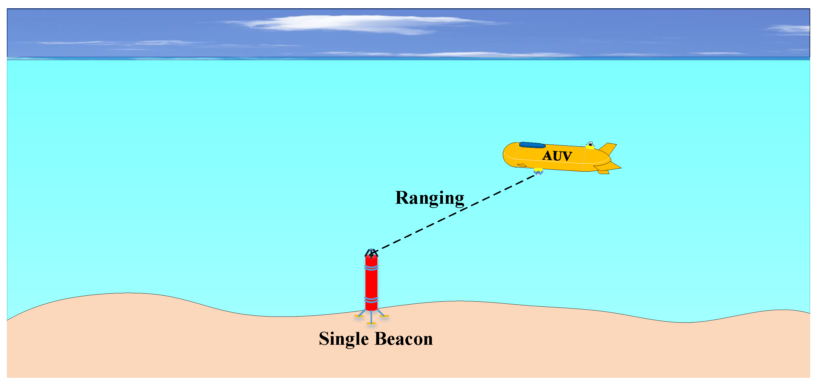
2.1. Framework of Single-Beacon Localization System
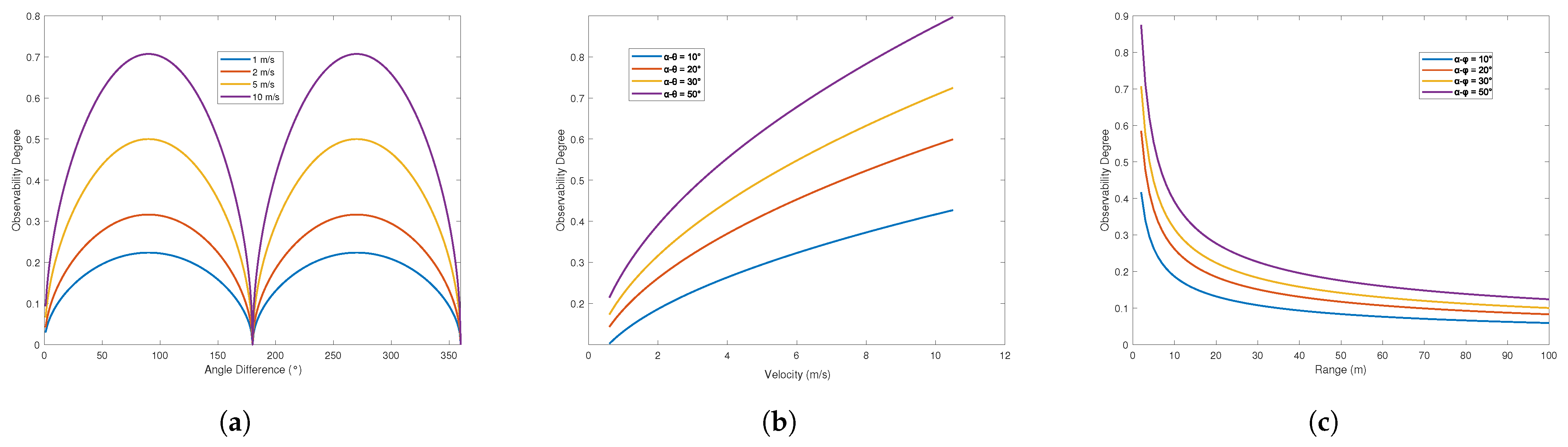
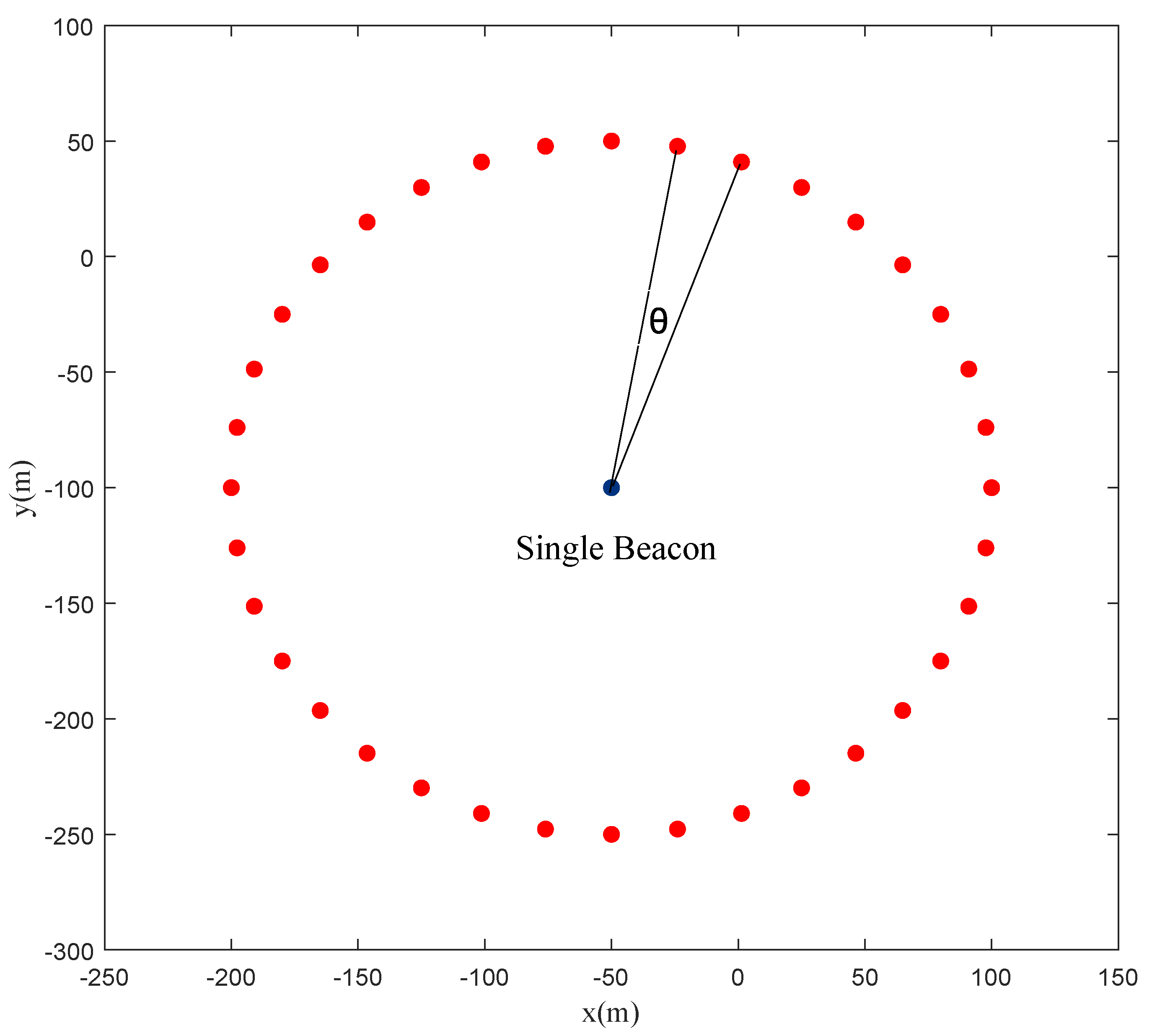
2.2. Observability Analysis
2.3. MHIPD
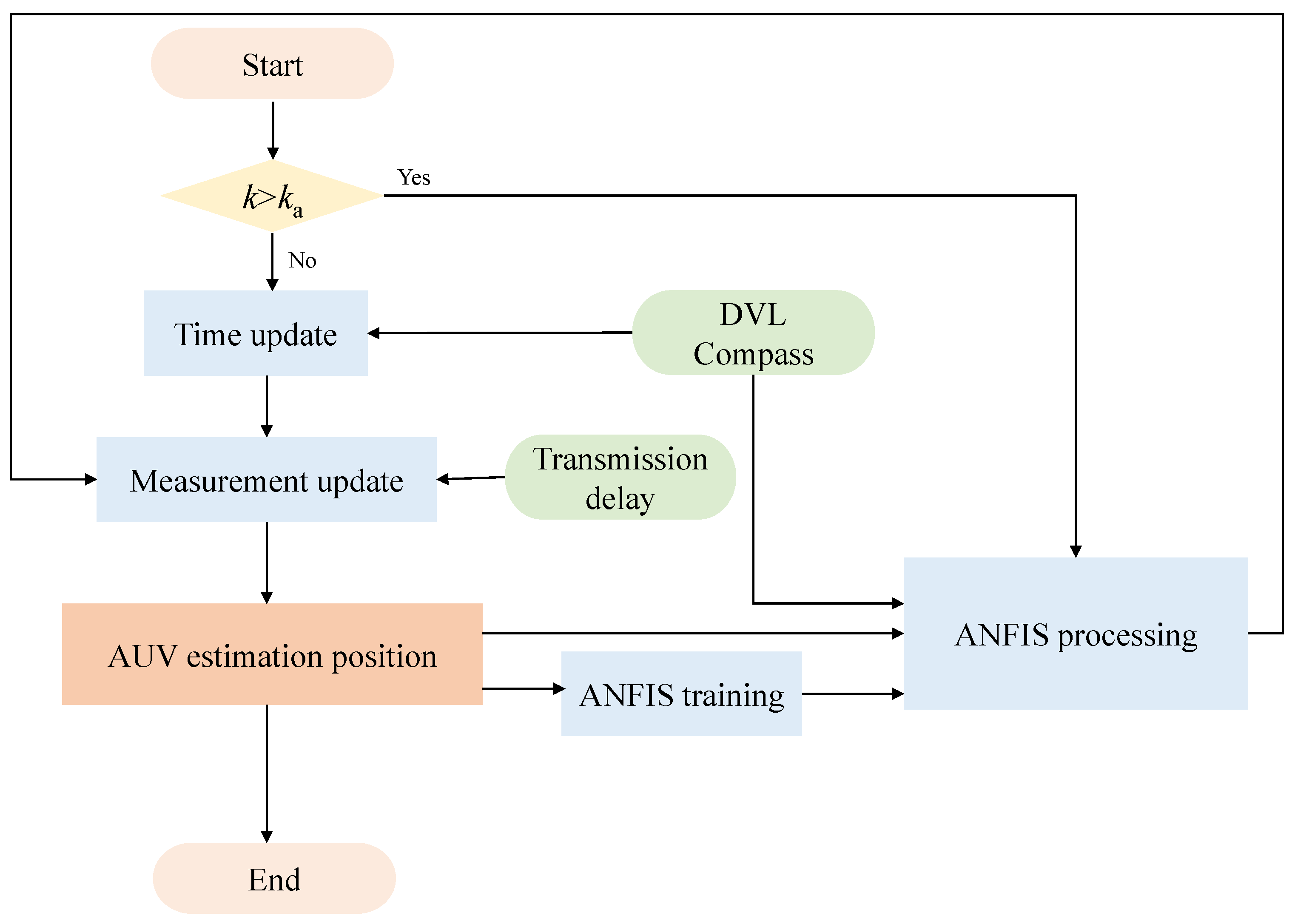
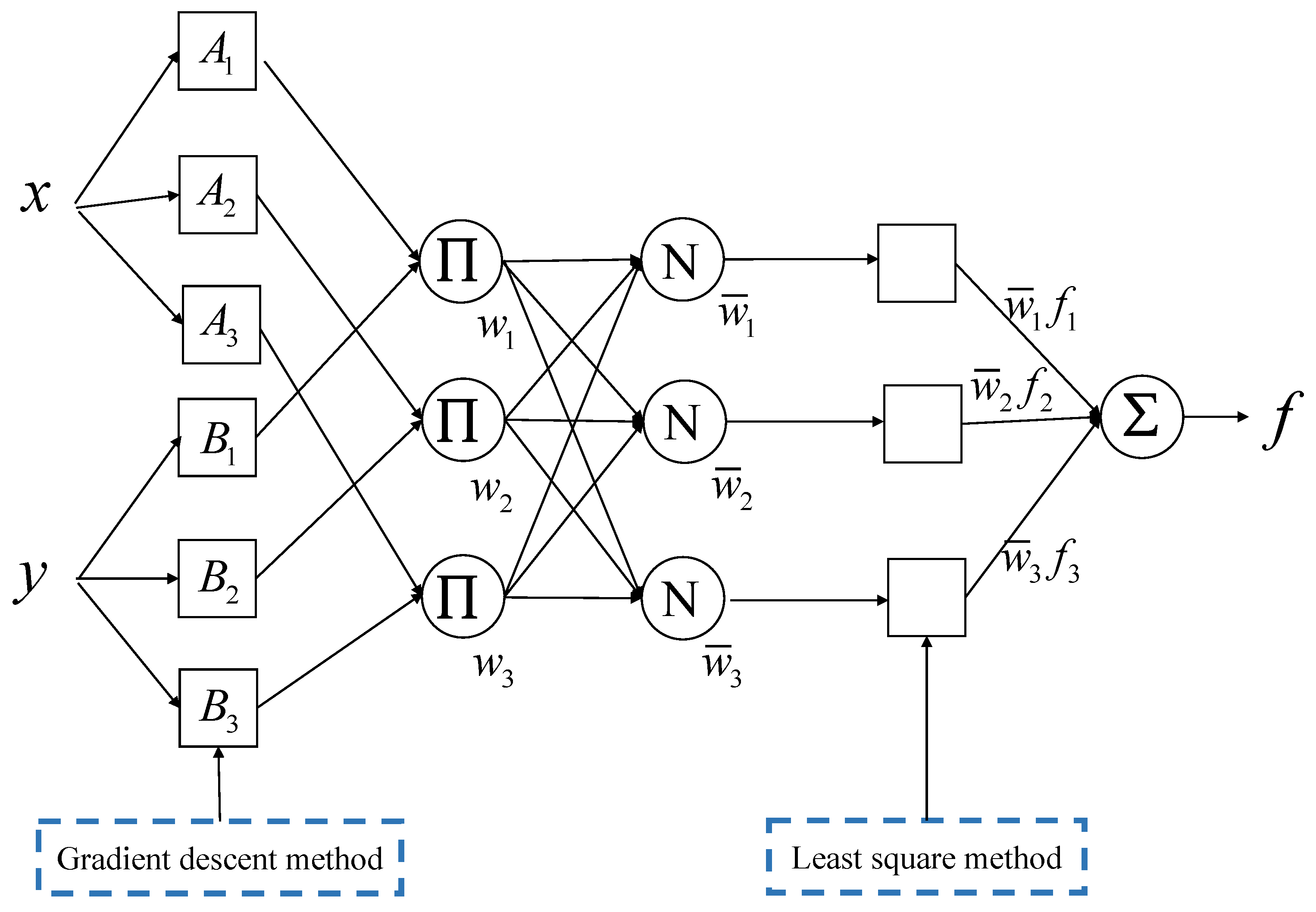
2.4. ANFIS-EKF
3. Results and Discussion
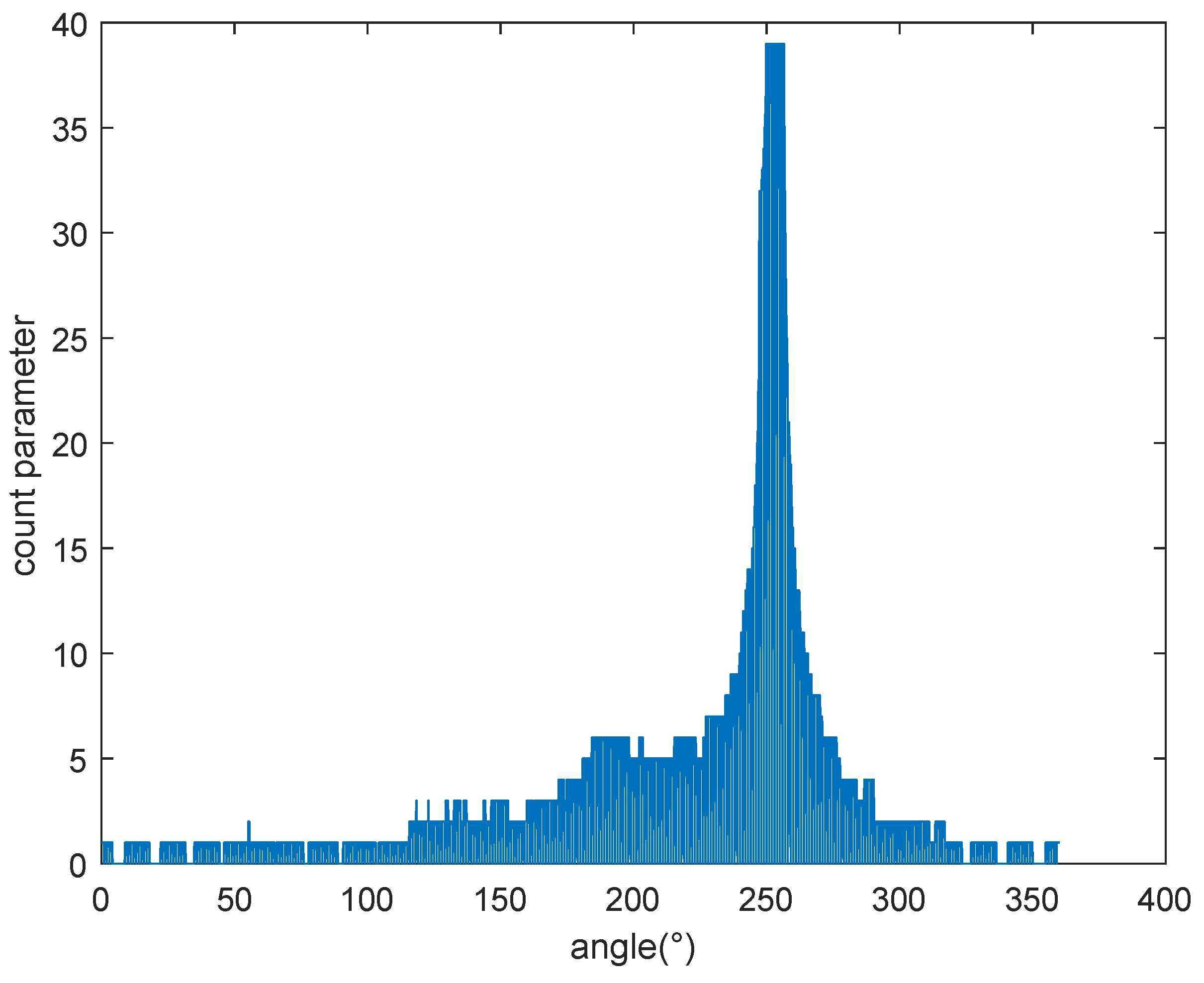
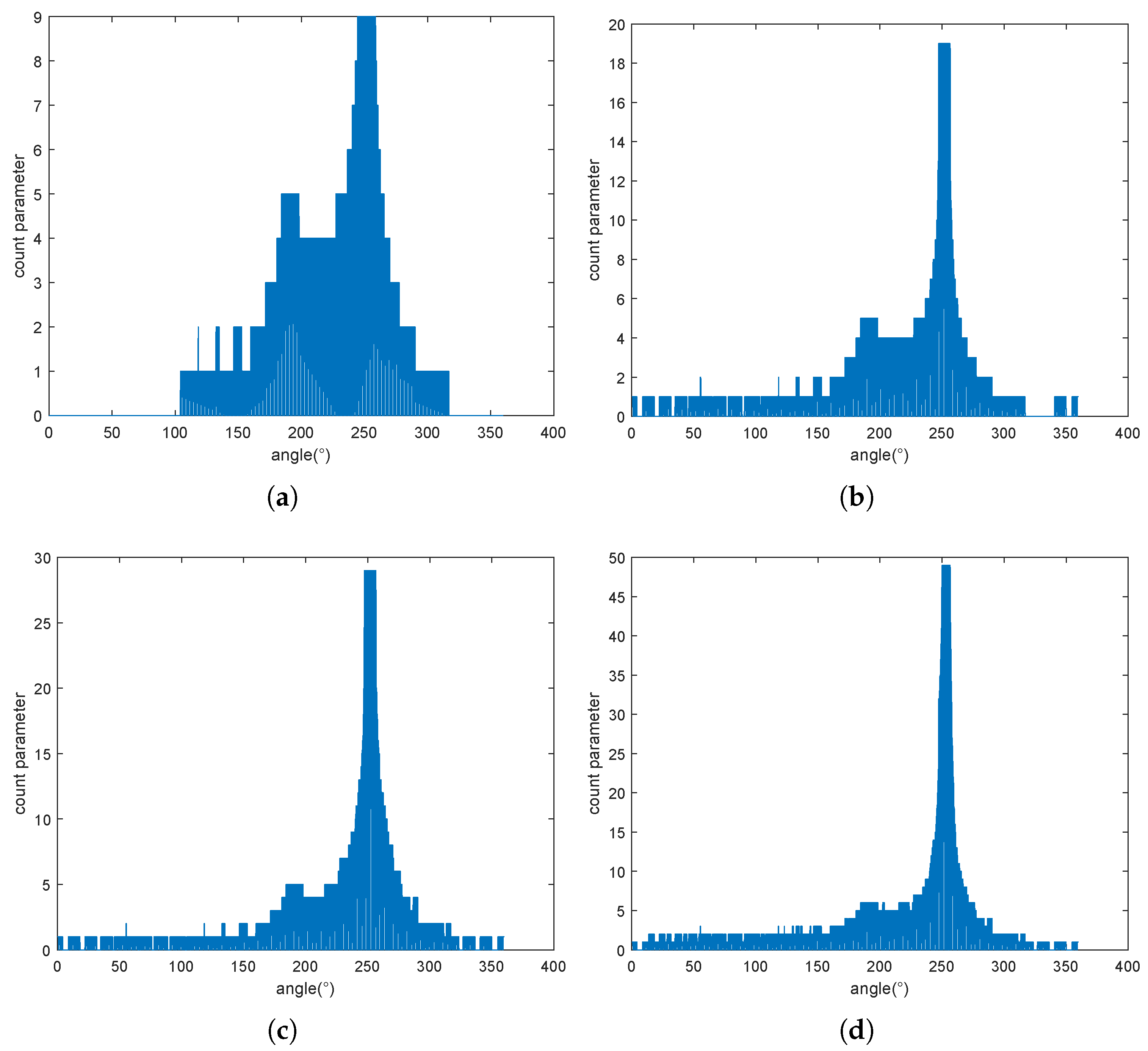
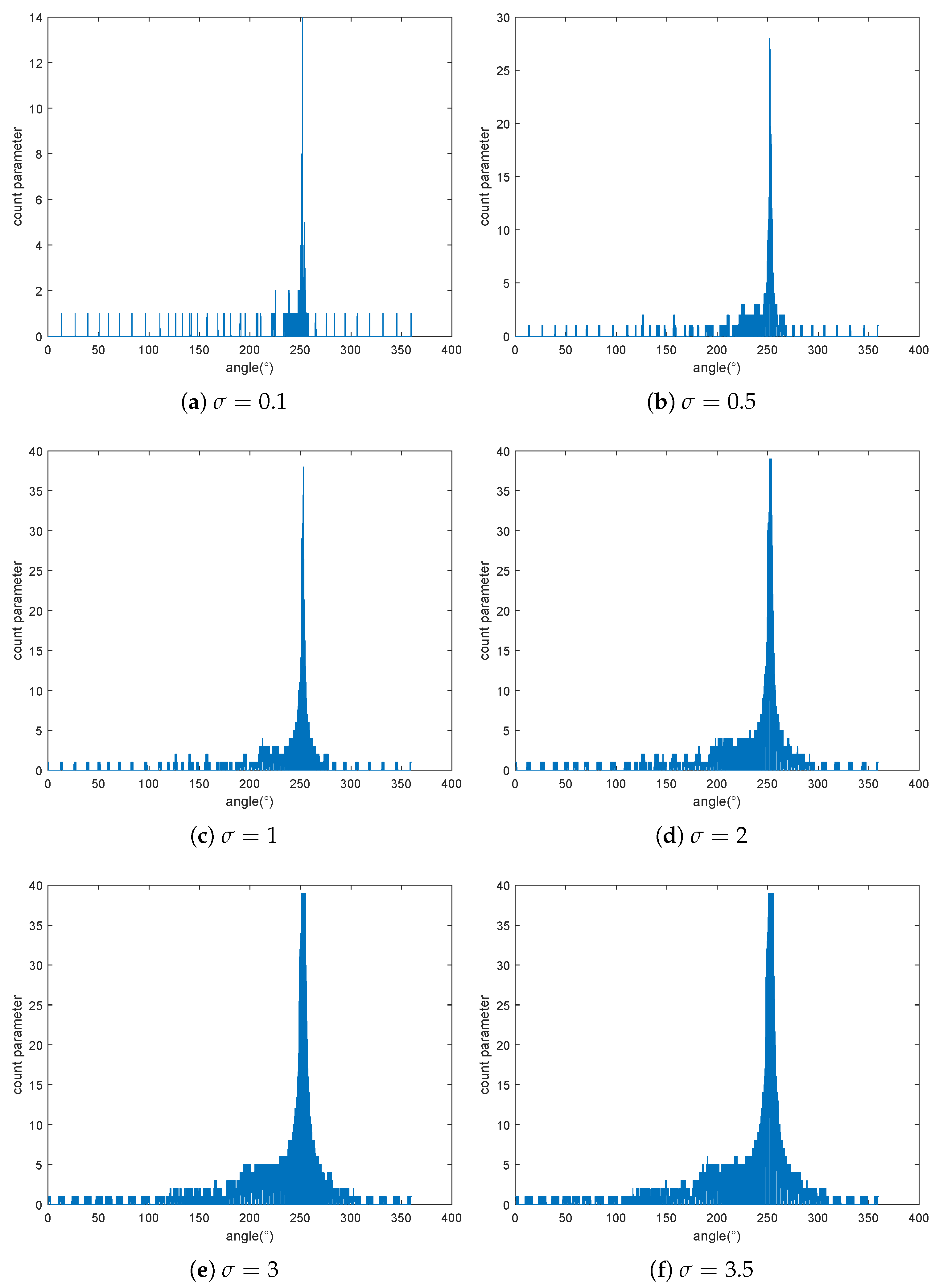
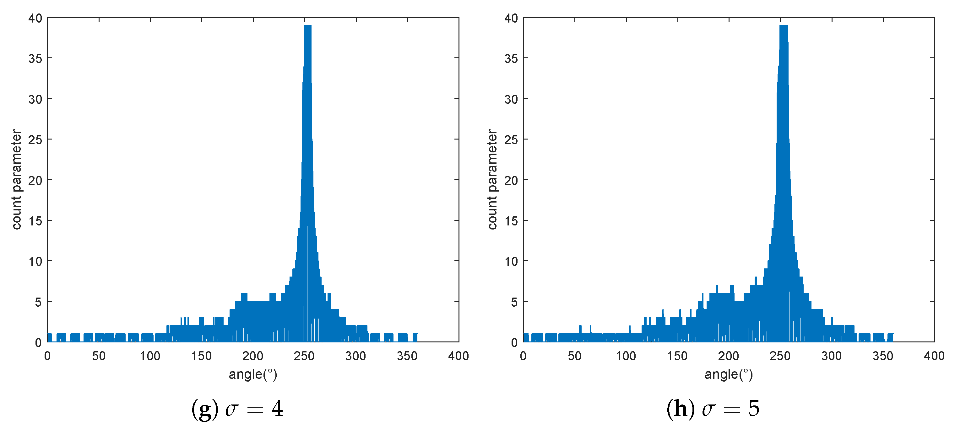
3.1. Performance Analysis of MHIPD
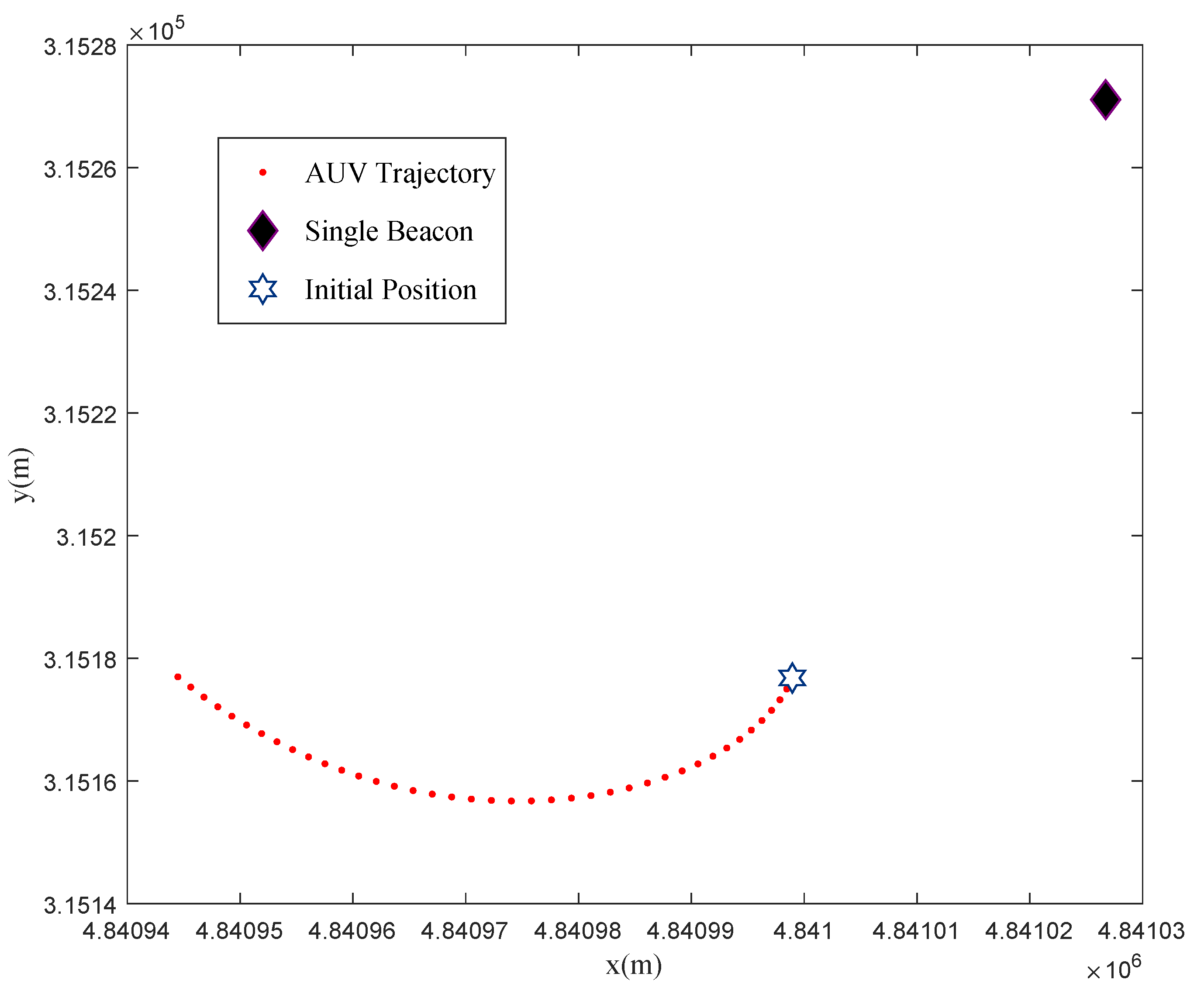
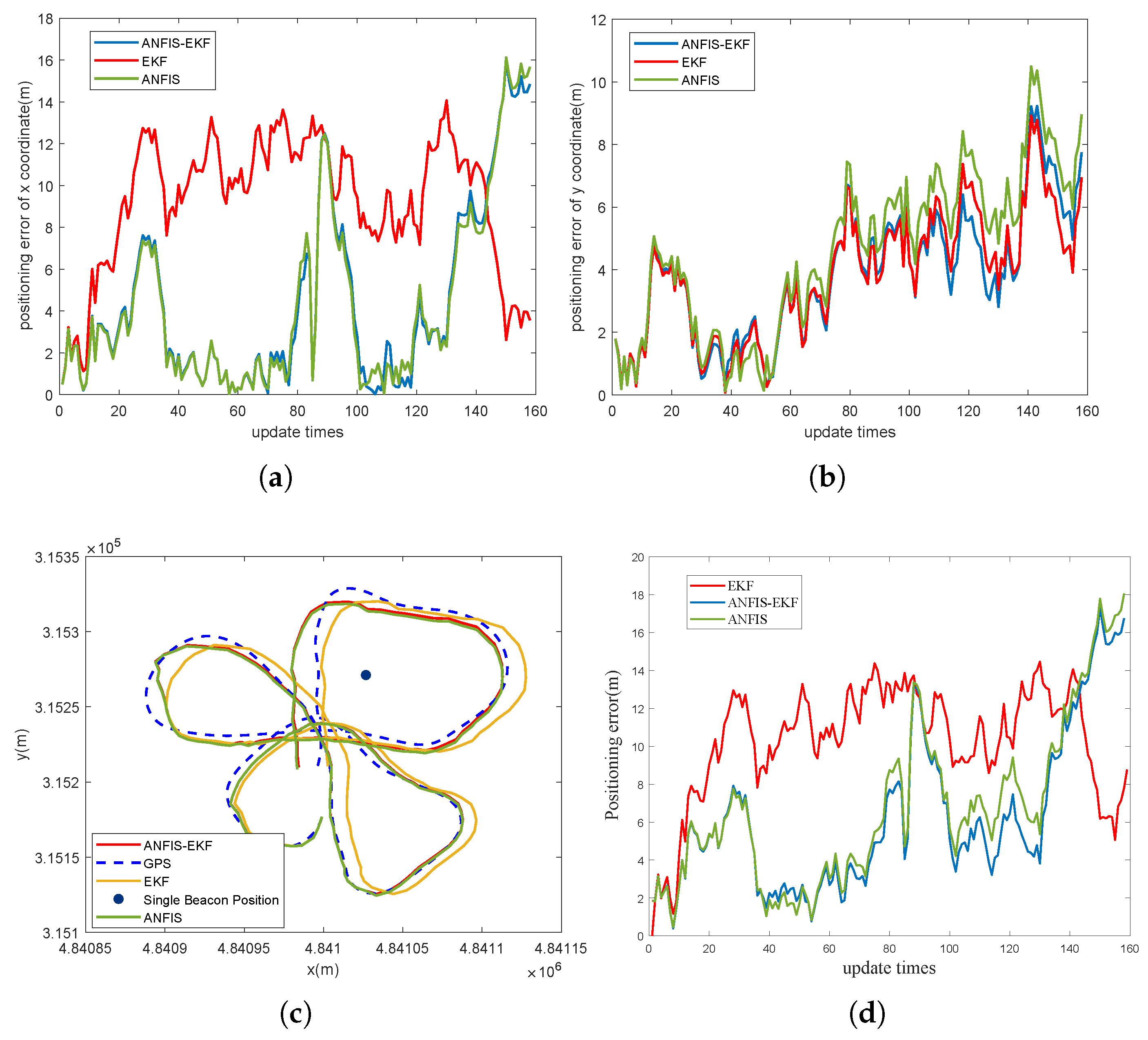
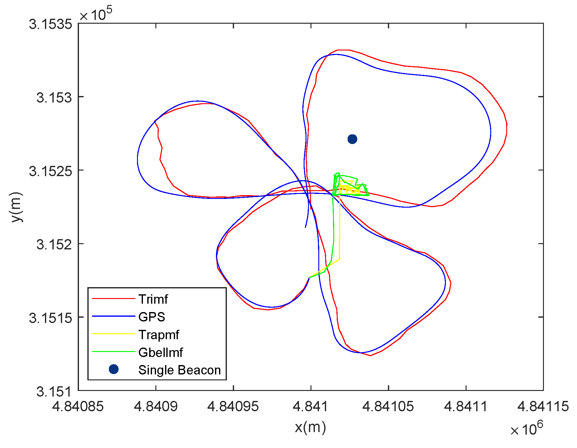
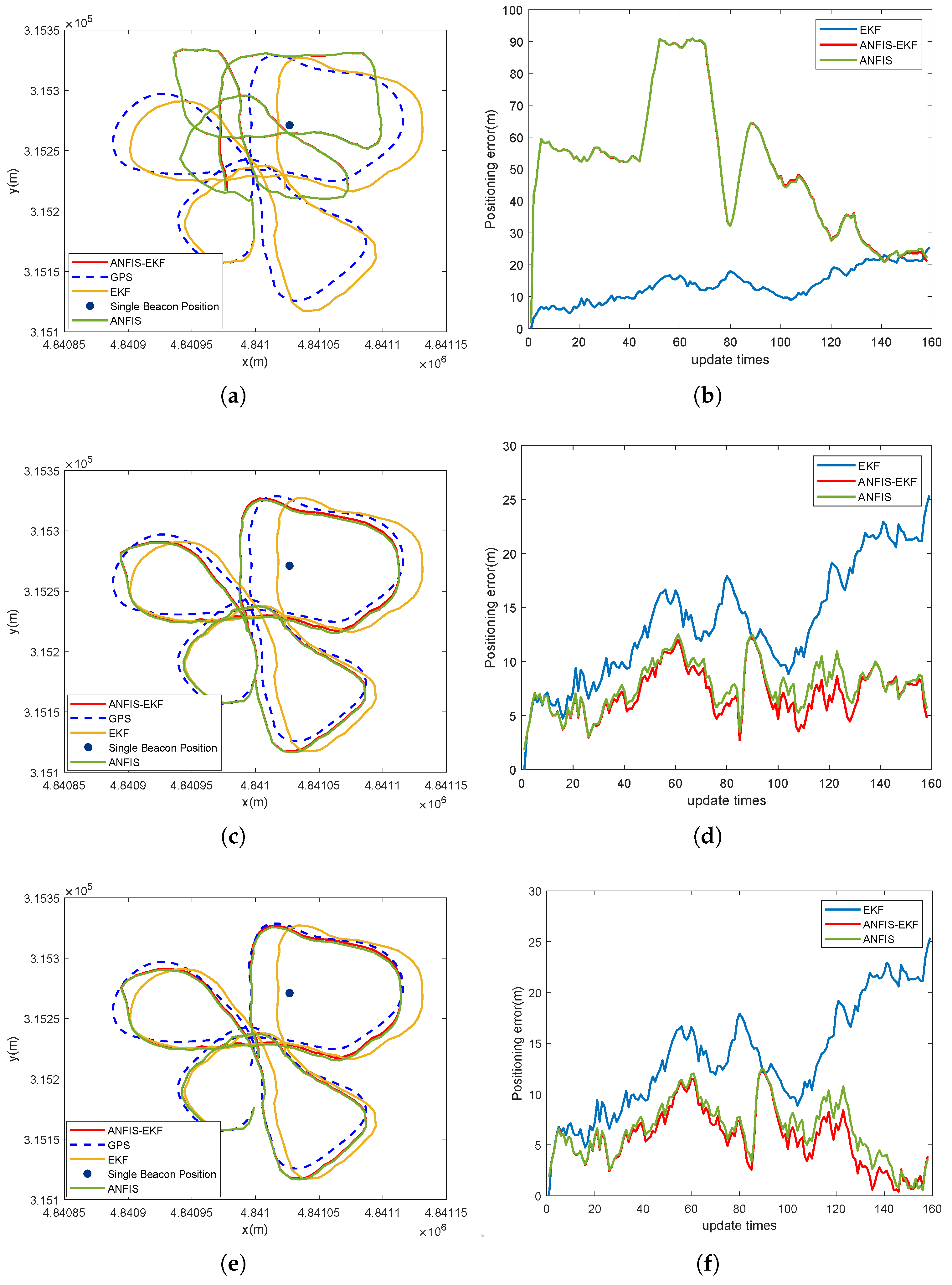
3.2. Performance Analysis of ANFIS-EKF
4. Conclusions
Author Contributions
Funding
Data Availability Statement
Conflicts of Interest
References
- Xing, H.; Liu, Y.; Guo, S.; Shi, L.; Hou, X.; Liu, W.; Zhao, Y. A Multi-Sensor Fusion Self-Localization System of a Miniature Underwater Robot in Structured and GPS-Denied Environments. IEEE Sens. J. 2021, 21, 27136–27146. [Google Scholar] [CrossRef]
- Scherbatyuk, A.P. The AUV positioning using ranges from one transponder LBL. In Proceedings of the OCEANS, ‘95 MTS/IEEE, San Diego, CA, USA, 9–12 October 1995; Volume 3, pp. 1620–1623. [Google Scholar]
- Vaganay, J.; Baccou, P.; Jouvencel, B. Homing by acoustic ranging to a single-beacon. In Proceedings of the OCEANS 2000 MTS/IEEE Conference and Exhibition, Providence, RI, USA, 11–14 September 2000; Volume 2, pp. 1457–1462. [Google Scholar]
- Vallicrosa, G.; Ridao, P. Sum of gaussian single-beacon range-only localization for AUV homing. Annu. Rev. Control 2016, 42, 177–187. [Google Scholar] [CrossRef]
- De Palma, D.; Arrichiello, F.; Parlangeli, G.; Indiveri, G. Underwater localization using single-beacon measurements: Observability analysis for a double integrator system. Ocean Eng. 2017, 142, 650–665. [Google Scholar] [CrossRef]
- Zhu, Z.B.; Hu, S.J. Model and algorithm improvement on single-beacon underwater tracking. IEEE J. Ocean. Eng. 2018, 43, 1143–1160. [Google Scholar] [CrossRef]
- Deng, Z.C.; Yu, X.; Qin, H.D.; Zhu, Z.B. Adaptive Kalman filter-based single-beacon underwater tracking with unknown effective sound velocity. Sensors 2018, 18, 4339. [Google Scholar] [CrossRef] [Green Version]
- Claus, B.; Kepper, J.H.; Suman, S.; Kinsey, J.C. Closed-loop one-way-travel-time navigation using low-grade odometry for autonomous underwater vehicles. J. Field Robot. 2018, 35, 421–434. [Google Scholar] [CrossRef] [Green Version]
- Qin, H.D.; Yu, X.; Zhu, Z.B.; Deng, Z.C. An expectation-maximization based single-beacon underwater navigation method with unknown ESV. Neurocomputing 2019, 378, 295–303. [Google Scholar] [CrossRef]
- Kepper, J.H.; Claus, B.C.; Kinsey, J.C. A navigation solution using a MEMS IMU, model-based dead-reckoning, and one-way-travel-time acoustic range measurements for autonomous underwater vehicles. IEEE J. Ocean. Eng. 2019, 44, 664–682. [Google Scholar] [CrossRef]
- Sun, J.; Hu, F.; Jin, W.M.; Wang, J.; Wang, X.; Luo, Y.; Yu, J.; Zhang, A. Model-aided localization and navigation for underwater gliders using single-beacon travel-time differences. Sensors 2020, 20, 893. [Google Scholar] [CrossRef] [Green Version]
- Yu, X.; Qin, H.D.; Zhu, Z.B. Globally exponentially stable single-beacon underwater navigation with unknown sound velocity estimation. J. Frankl. Inst. Eng. Appl. Math. 2021, 358, 2515–2534. [Google Scholar] [CrossRef]
- Masmitja, I.; Gomariz, S.; Del-Rio, J.; Kieft, B.; O’Reilly, T.; Bouvet, P.J.; Aguzzi, J. Optimal path shape for range-only underwater target localization using a wave glider. Int. J. Robot. Res. 2018, 37, 1447–1462. [Google Scholar] [CrossRef] [Green Version]
- Liu, H.M.; Wang, Z.J.; Zhao, S.; He, K. Accurate multiple ocean bottom seismometer positioning in shallow water using GNSS/Acoustic Technique. Sensors 2019, 19, 1406. [Google Scholar] [CrossRef] [PubMed] [Green Version]
- Rahman, A.; Muthukkumarasamy, V. Embracing localization inaccuracy with a single-beacon. Int. J. Adv. Comput. Sci. Appl. 2019, 10, 452–459. [Google Scholar] [CrossRef] [Green Version]
- Sun, S.B.; Zhang, X.Y.; Zheng, C.; Fu, J.; Zhao, C. Underwater acoustical localization of the black box utilizing single autonomous underwater vehicle based on the second-order time difference of arrival. IEEE J. Ocean. Eng. 2020, 45, 1268–1279. [Google Scholar] [CrossRef]
- Sun, S.B.; Zhang, X.Y.; Zheng, C.; Zhao, C.; Fu, J. Underwater asynchronous navigation using single-beacon based on the phase difference. Appl. Acoust. 2021, 172, 107546. [Google Scholar] [CrossRef]
- Larsen, M.B. Synthetic long baseline navigation of underwater vehicles. In Proceedings of the OCEANS 2000 MTS/IEEE Conference and Exhibition, Providence, RI, USA, 11–14 September 2000; Volume 3, pp. 2043–2050. [Google Scholar]
- Lapointe C, E. Virtual Long Baseline (VLBL) Autonomous Underwater Vehicle Navigation Using a Single Transponder; Massachusetts Institute of Technology: Cambridge, MA, USA, 2006. [Google Scholar]
- Cao, J.; Han, Y.F.; Zhang, D.L.; Sun, D. Linearized iterative method for determining effects of vessel attitude error on single-beacon localization. Appl. Acoust. 2017, 116, 297–302. [Google Scholar] [CrossRef]
- Masmitja, I.; Bouvet, P.J.; Gomariz, S.; Aguzzi, J.; del Rio, J. Underwater mobile target tracking with particle filter using an autonomous vehicle. In Proceedings of the OCEANS 2017, Aberdeen, UK, 19–22 June 2017; pp. 1–5. [Google Scholar]
- Shaukat, N.; Ali, A.; Javed, I.M.; Moinuddin, M.; Orero, P. Multi-Sensor Fusion for Underwater Vehicle Localization by Augmentation of RBF Neural Network and Error-State Kalman Filter. Sensors 2021, 21, 1149. [Google Scholar] [CrossRef] [PubMed]
- Ma, H.; Mu, X.; He, B. Adaptive Navigation Algorithm with Deep Learning for Autonomous Underwater Vehicle. Sensors 2021, 21, 6406. [Google Scholar] [CrossRef]
- Or, B.; Klein, I. Adaptive Step Size Learning with Applications to Velocity Aided Inertial Navigation System. IEEE Access 2022, 10, 85818–85830. [Google Scholar] [CrossRef]
- Jang, J.R. ANFIS: Adaptive-network-based fuzzy inference system. IEEE Trans. Syst. Man Cybern. 1993, 23, 665–685. [Google Scholar] [CrossRef]
- Gharghan, S.K.; Nordin, R.; Ismail, M. A wireless sensor network with soft computing localization techniques for track cycling applications. Sensors 2016, 16, 1043. [Google Scholar] [CrossRef] [PubMed] [Green Version]
- Duan, Y.B.; Li, H.Z.; Wu, S.Q.; Zhang, K. INS error estimation based on an ANFIS and its application in complex and covert surroundings. ISPRS Int. J. Geo-Inf. 2021, 10, 388. [Google Scholar] [CrossRef]
- Taek, L.S. Observability of target tracking with range-only measurements. IEEE J. Ocean. Eng. 1999, 24, 383–387. [Google Scholar] [CrossRef]
- Kabir, M.; Kabir, M.M.J. Fuzzy membership function design: An adaptive neuro-fuzzy inference system (ANFIS) based approach. In Proceedings of the 2021 International Conference on Computer Communication and Informatics (ICCCI), Coimbatore, India, 27–29 January 2021; pp. 1–5. [Google Scholar]


| Parameters | Value |
|---|---|
| Initial fuzzy inference system for training | Grid Partition |
| Input membership function type | trimf |
| Output membership function type | linear |
| Training length | 150 |
| Number of Input membership function | 3 |
| Error Goal | 0.0001 |
| Calculating Times k | Error of RMSE (m) | Number of Max Count Parameter | Angle of Initial Position (∘) |
|---|---|---|---|
| 10 | 3.5439 | 128 | 251.6 |
| 20 | 3.2111 | 85 | 251.8 |
| 30 | 3.2111 | 84 | 251.8 |
| 50 | 1.1089 | 60 | 253.2 |
| Threshold Value | Error of RMSE (m) | Number of Max Count Parameter | Angle of Initial Position (∘) |
|---|---|---|---|
| 0.1 | 3.0457 | 1 | 251.9 |
| 0.5 | 2.5551 | 6 | 252.2 |
| 1.0 | 1.7710 | 2 | 252.7 |
| 2.0 | 1.4817 | 19 | 252.9 |
| 3.0 | 1.3469 | 36 | 253.0 |
| 3.5 | 1.2215 | 45 | 253.1 |
| 4.0 | 1.2215 | 53 | 253.1 |
| 5.0 | 1.1089 | 69 | 253.2 |
| Method | Error of x Direction (m) | Error of y Direction (m) | Error of DRMS (m) |
|---|---|---|---|
| EKF | 9.2260 | 3.8170 | 10.3271 |
| ANFIS | 4.3264 | 4.5613 | 6.7529 |
| ANFIS-EKF | 4.3275 | 3.8053 | 6.1890 |
| Method | Error of 80 Length (m) | Error of 120 Length (m) | Error of 150 Length (m) |
|---|---|---|---|
| EKF | 13.6391 | 13.6391 | 13.6391 |
| ANFIS | 50.4973 | 7.7264 | 6.4113 |
| ANFIS-EKF | 50.1967 | 7.0206 | 5.6006 |
Publisher’s Note: MDPI stays neutral with regard to jurisdictional claims in published maps and institutional affiliations. |
© 2022 by the authors. Licensee MDPI, Basel, Switzerland. This article is an open access article distributed under the terms and conditions of the Creative Commons Attribution (CC BY) license (https://creativecommons.org/licenses/by/4.0/).
Share and Cite
Zhao, W.; Zhao, H.; Liu, G.; Zhang, G. ANFIS-EKF-Based Single-Beacon Localization Algorithm for AUV. Remote Sens. 2022, 14, 5281. https://doi.org/10.3390/rs14205281
Zhao W, Zhao H, Liu G, Zhang G. ANFIS-EKF-Based Single-Beacon Localization Algorithm for AUV. Remote Sensing. 2022; 14(20):5281. https://doi.org/10.3390/rs14205281
Chicago/Turabian StyleZhao, Wanlong, Huifeng Zhao, Gongliang Liu, and Guoyao Zhang. 2022. "ANFIS-EKF-Based Single-Beacon Localization Algorithm for AUV" Remote Sensing 14, no. 20: 5281. https://doi.org/10.3390/rs14205281