
Developing a Dual-Stream Deep-Learning Neural Network Model for Improving County-Level Winter Wheat Yield Estimates in China
 , ,
, ,  ,
,
Abstract
:1. Introduction
2. Study Area and Dataset
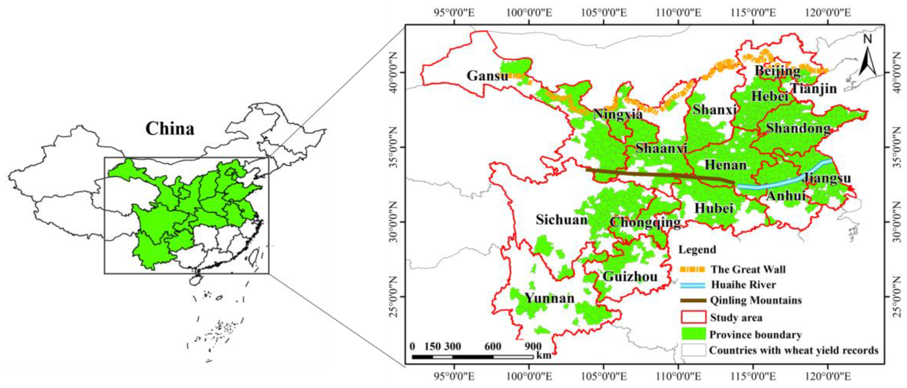
2.1. Study Area
2.2. Dataset
2.2.1. Remote-Sensing Data
2.2.2. Weather Data
2.2.3. Soil Property Data
2.2.4. Cropland Land Cover Data
2.2.5. County-Level Yield Data
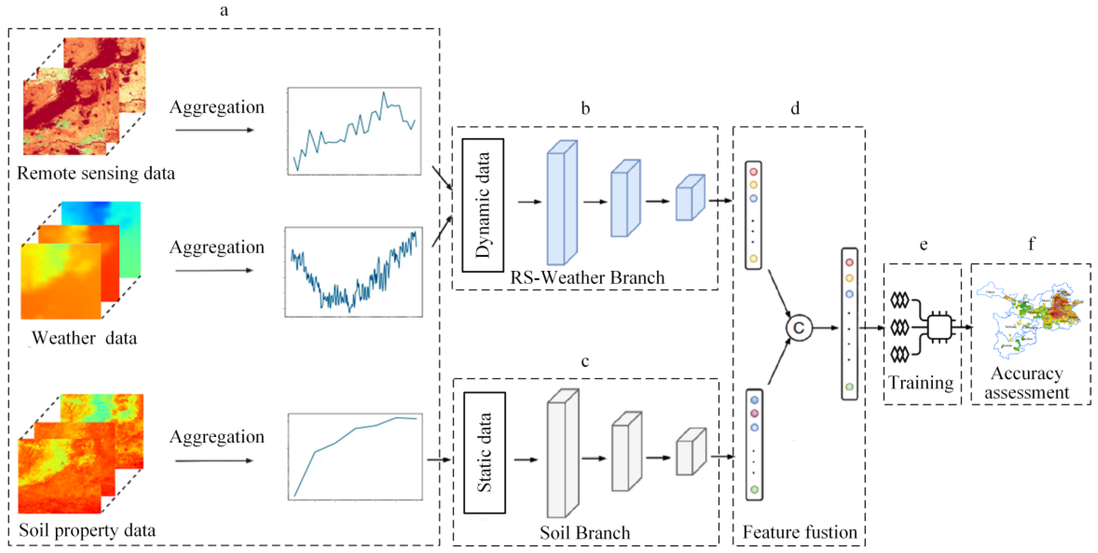
3. Methods
3.1. Data Preprocessing
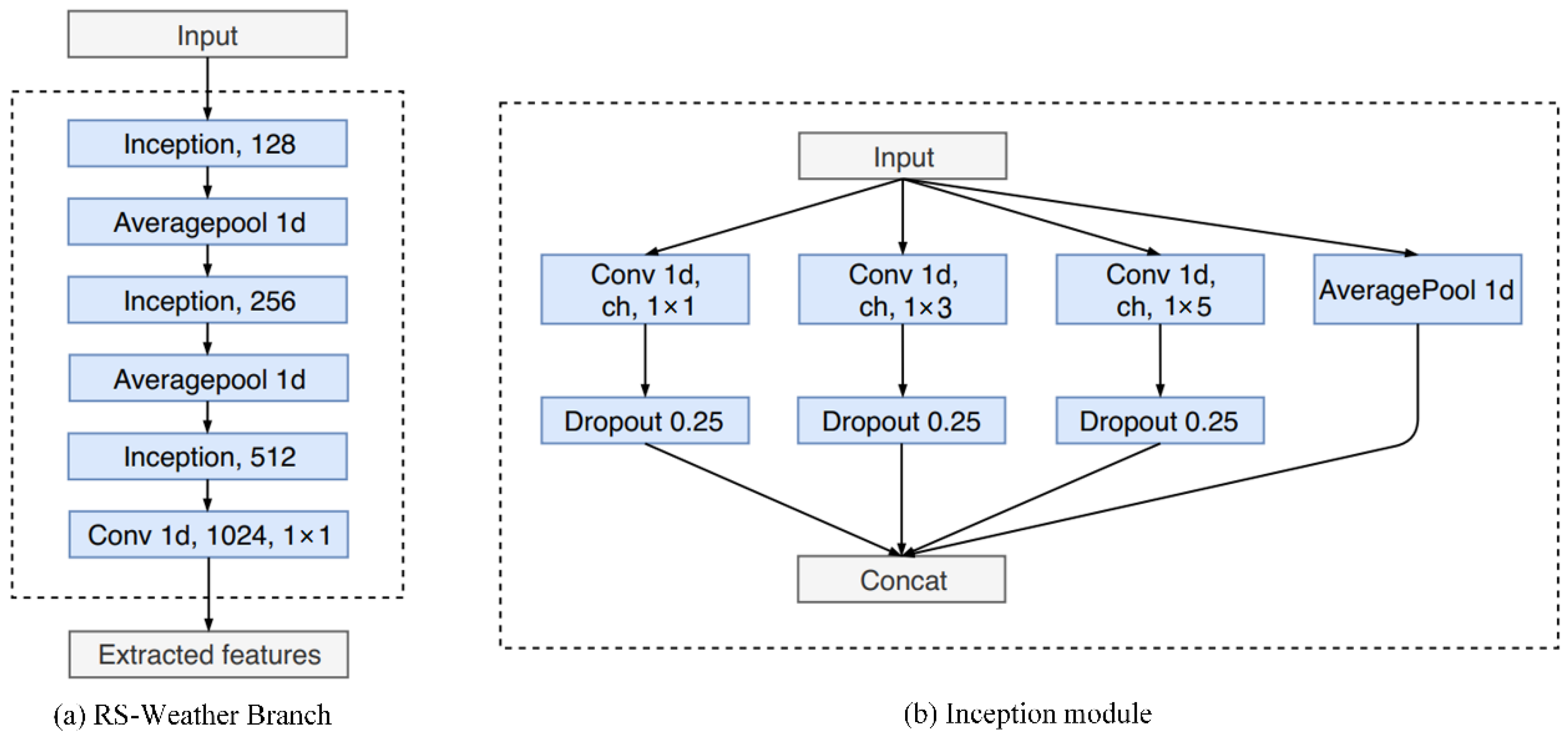
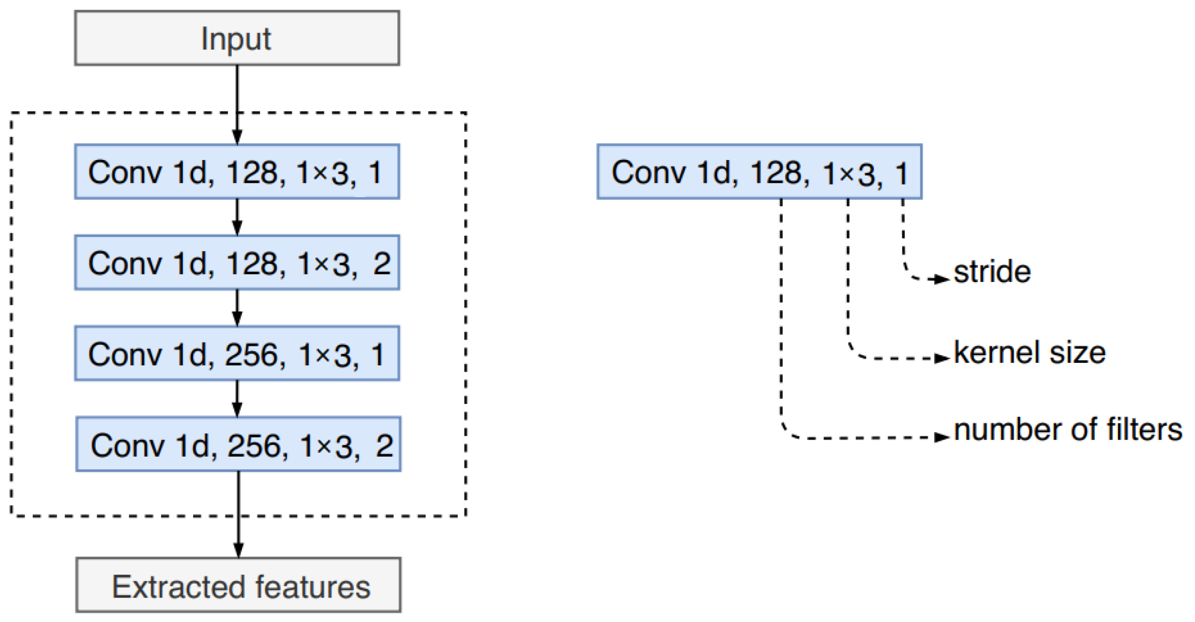
3.2. Remote-Sensing–Weather Branch
3.3. Soil Branch
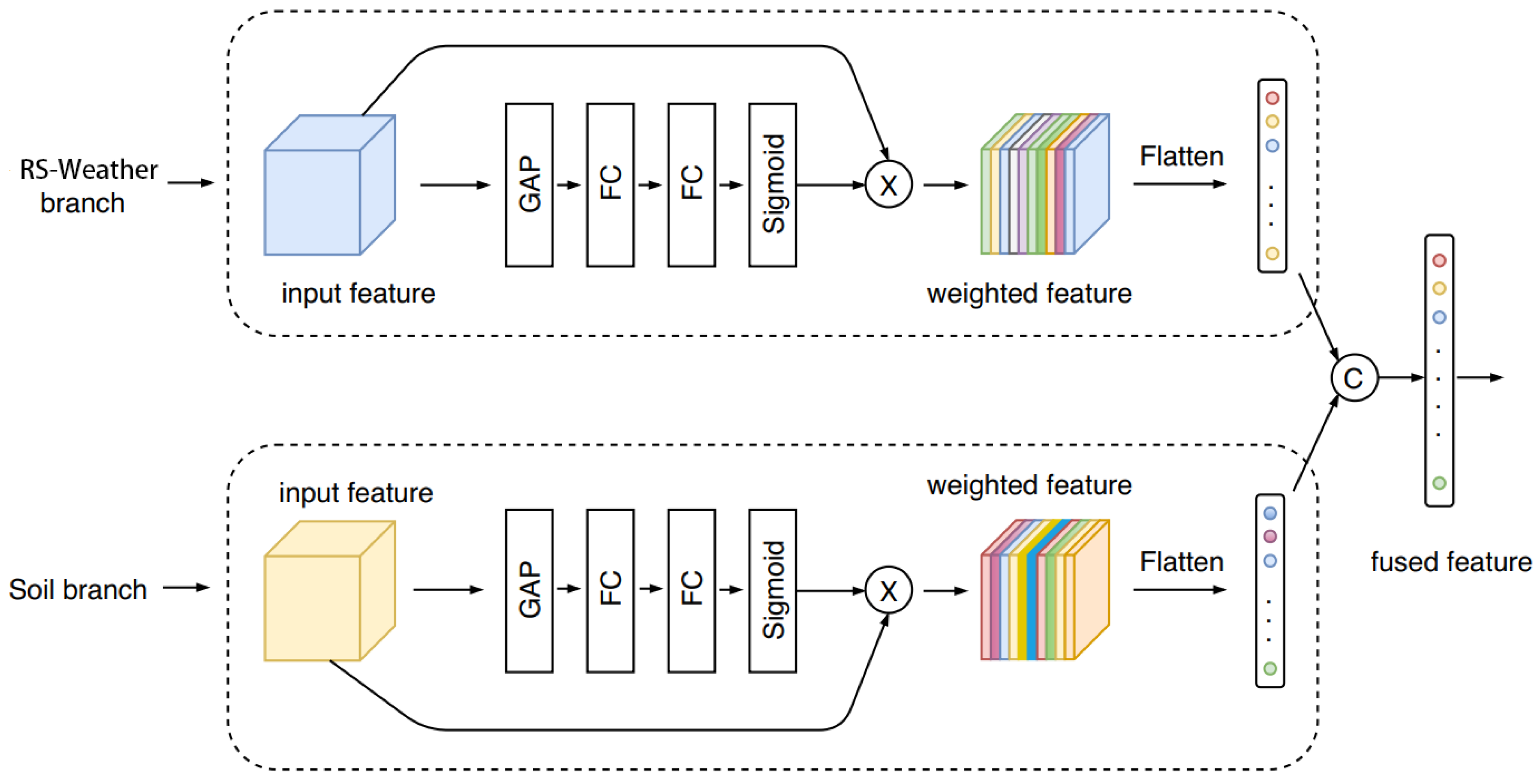
3.4. Fusion Module
3.5. Network Training
3.6. Accuracy Assessment
4. Results
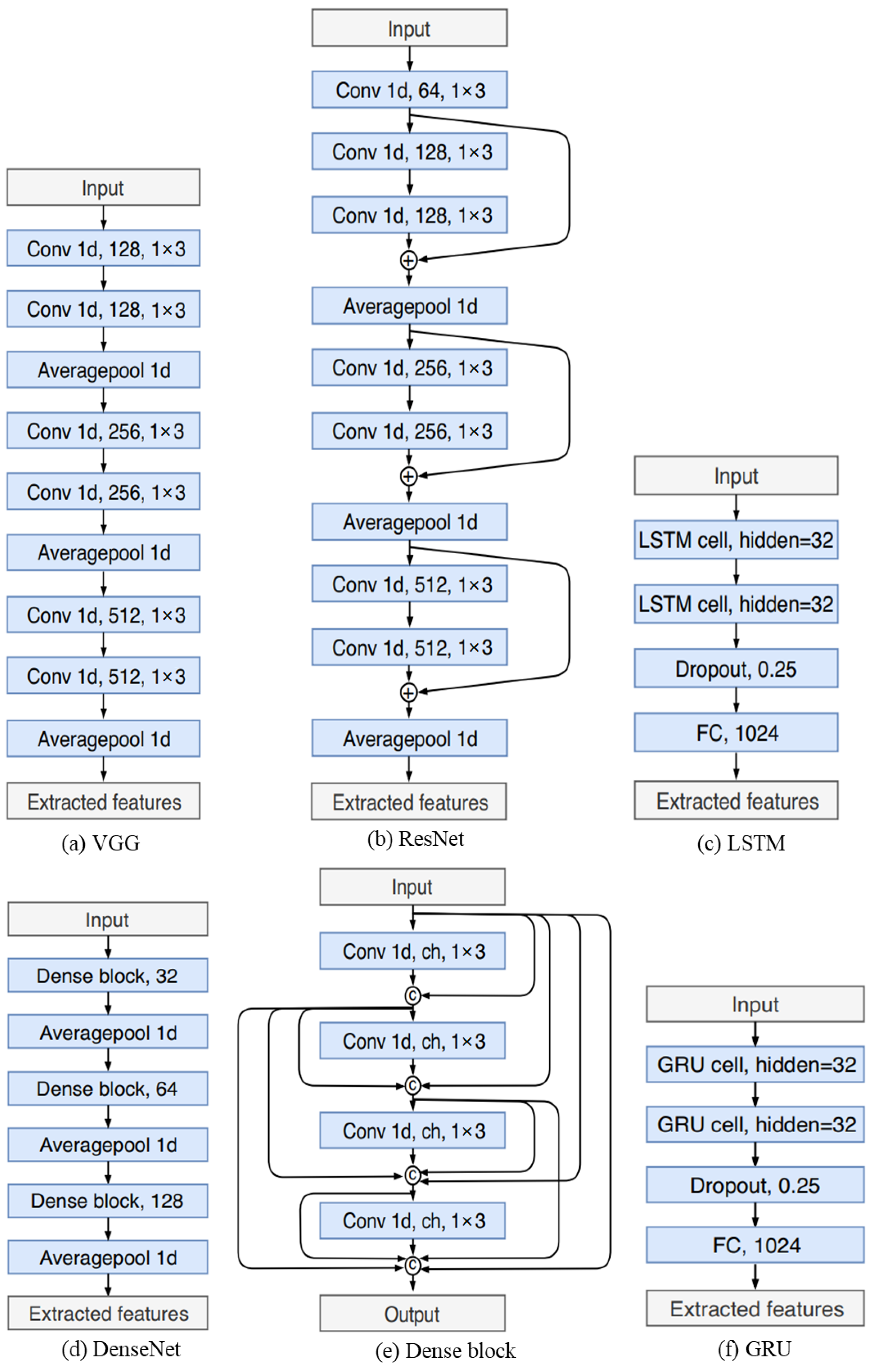
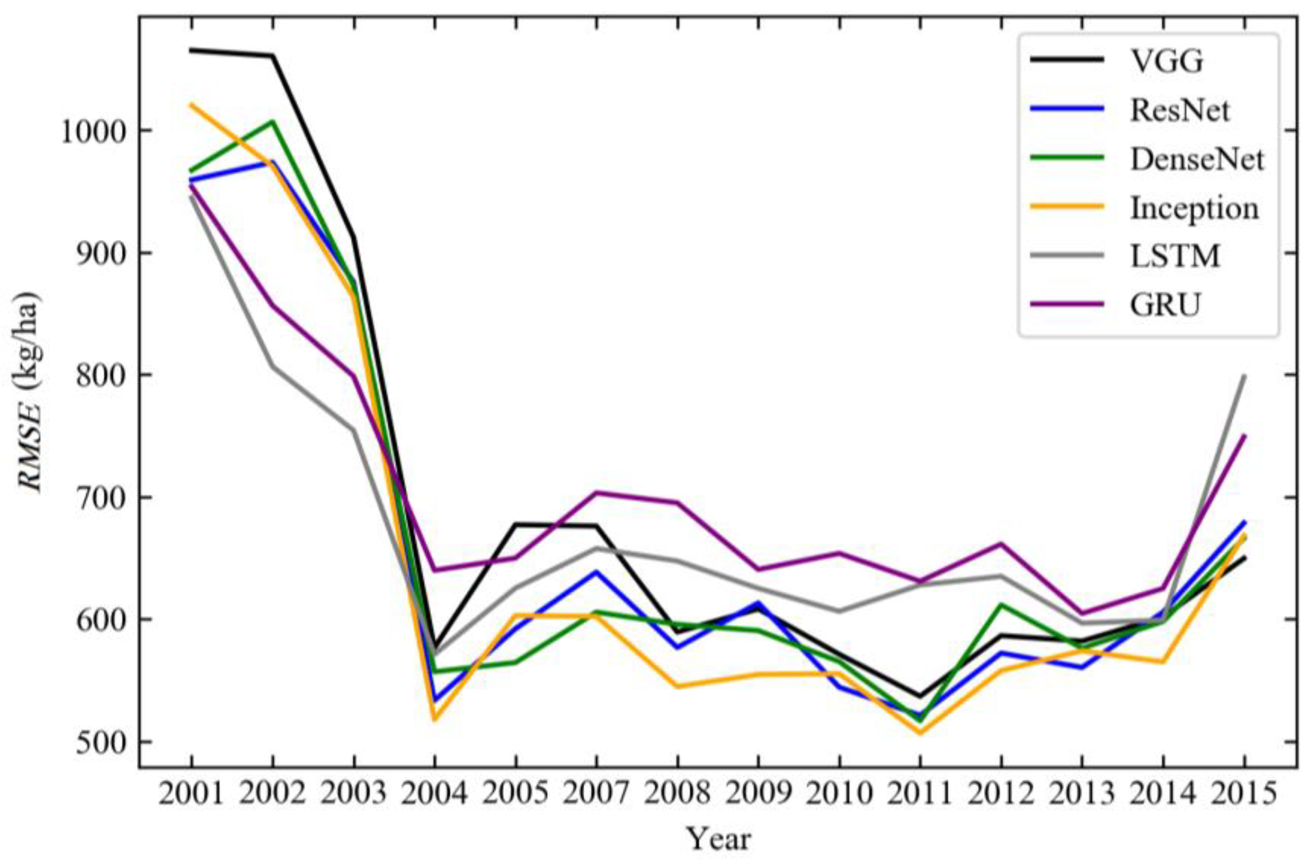
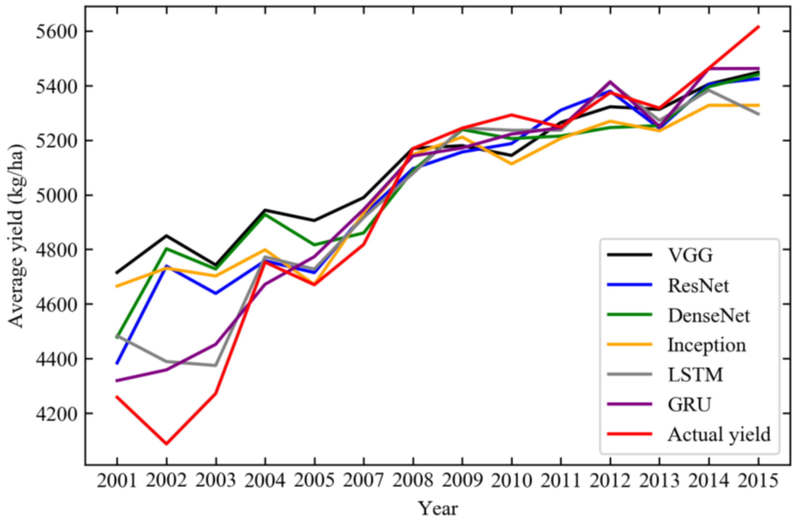
4.1. Comparing Different Deep-Learning Models to Predict Winter Wheat Yield
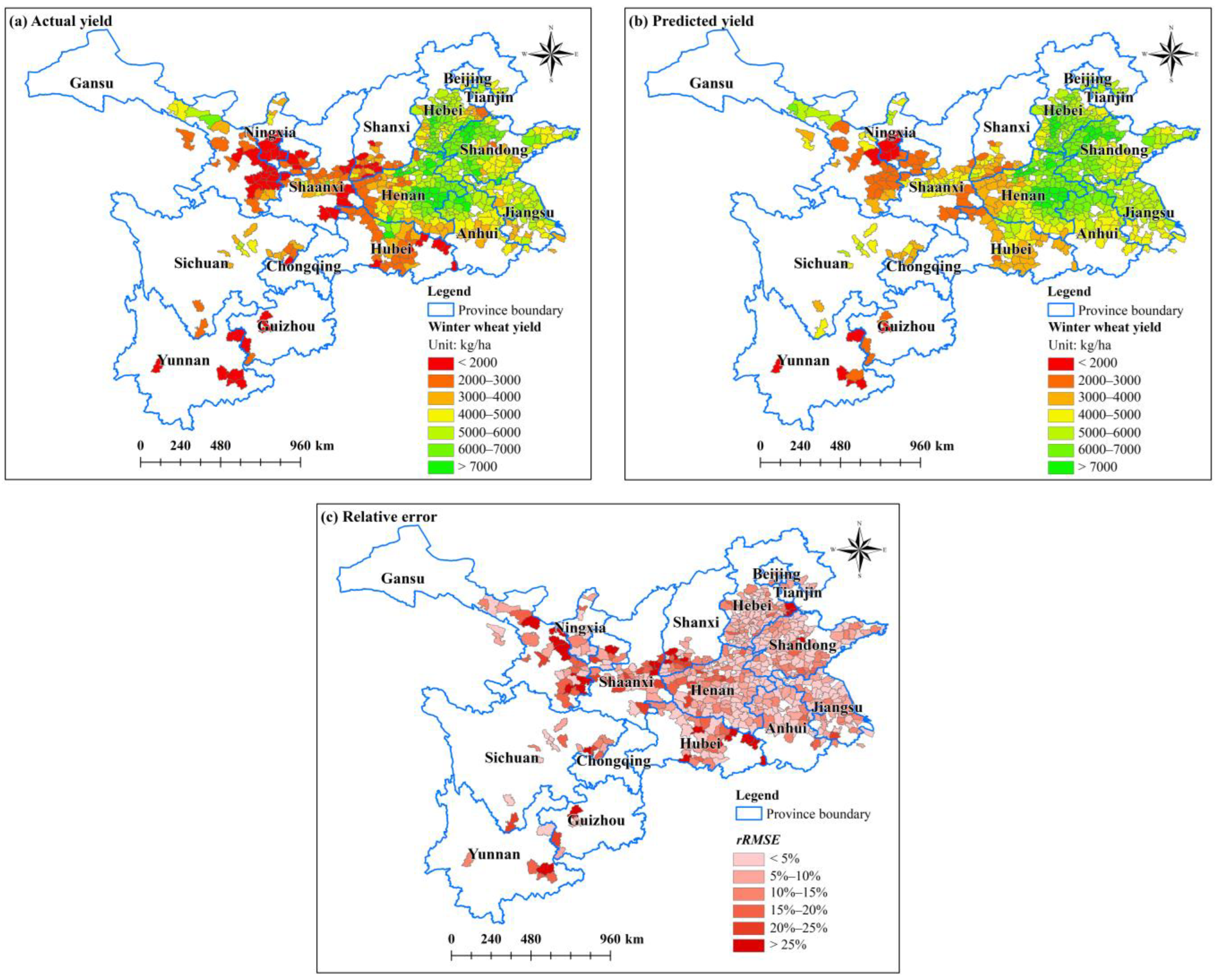
4.2. Spatial Variation in Winter Wheat Yield Predictions
5. Discussion
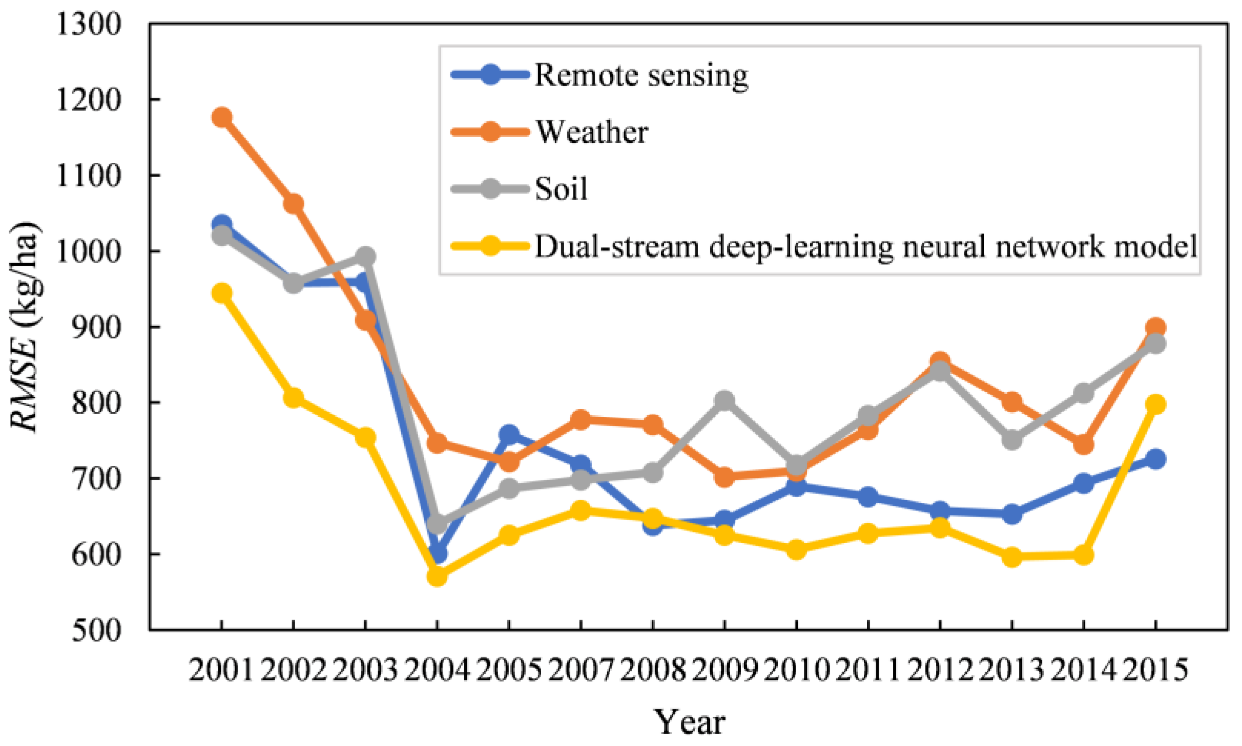
5.1. Impact of Different Data Sources on Winter Wheat Yield Prediction
5.2. Comparison with Traditional Methods
5.3. Comparison with Other Deep-Learning Yield-Prediction Methods
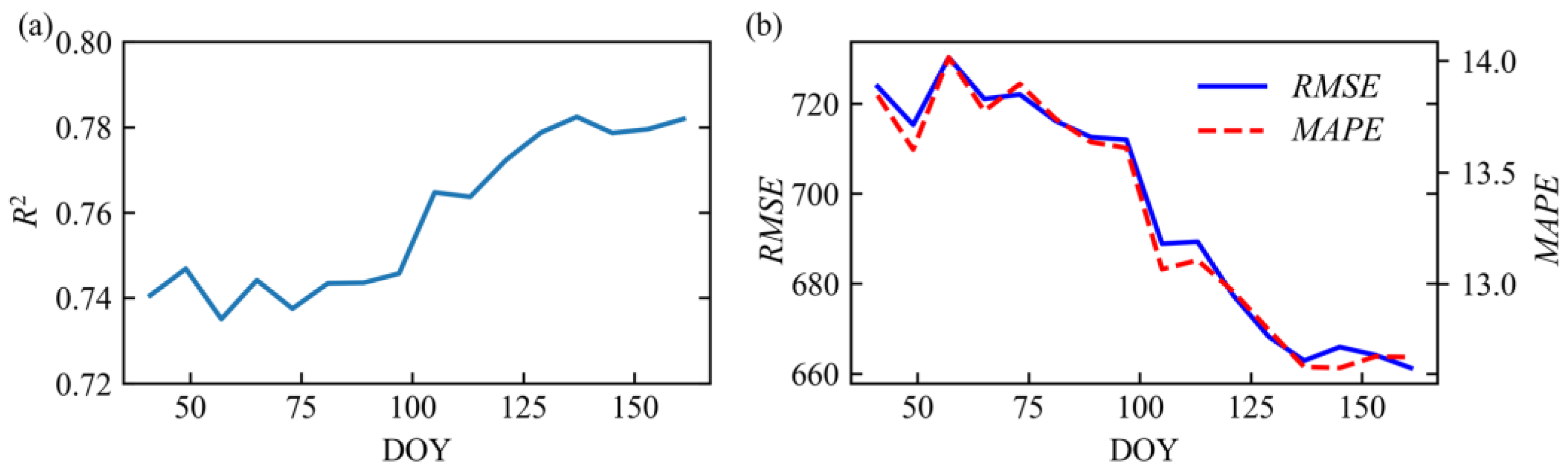
5.4. In-Season Winter Wheat Yield Prediction
5.5. Possibility of Establishing a Parcel-Level Crop Yield-Prediction Model
5.6. Limitations and Future Perspective
6. Conclusions
Author Contributions
Funding
Data Availability Statement
Acknowledgments
Conflicts of Interest
References
- Benami, E.; Jin, Z.; Carter, M.R.; Ghosh, A.; Hijmans, R.J.; Hobbs, A.; Kenduiywo, B.; Lobell, D.B. Uniting remote sensing, crop modelling and economics for agricultural risk management. Nat. Rev. Earth Environ. 2021, 2, 140–159. [Google Scholar] [CrossRef]
- FAO. The future of food and agriculture—Trends and challenges. Annu. Rep. 2017, 296, 1–180. [Google Scholar]
- Cui, K.; Shoemaker, S.P. A look at food security in China. Nat. Publ. Group 2018, 2, 4. [Google Scholar] [CrossRef] [PubMed] [Green Version]
- Doraiswamy, P.C.; Moulin, S.; Cook, P.W.; Stern, A. Crop yield assessment from remote sensing. Photogramm. Eng. Remote Sens. 2003, 69, 665–674. [Google Scholar] [CrossRef]
- Basso, B.; Liu, L. Seasonal crop yield forecast: Methods, applications, and accuracies. Adv. Agron. 2019, 154, 201–255. [Google Scholar]
- Huang, J.; Gómez-Dans, J.L.; Huang, H.; Ma, H.; Wu, Q.; Lewis, P.E.; Liang, S.; Chen, Z.; Xue, J.; Wu, Y. Assimilation of remote sensing into crop growth models: Current status and perspectives. Agric. For. Meteorol. 2019, 276, 107609. [Google Scholar] [CrossRef]
- Becker-Reshef, I.; Vermote, E.; Lindeman, M.; Justice, C. A generalized regression-based model for forecasting winter wheat yields in Kansas and Ukraine using MODIS data. Remote Sens. Environ. 2010, 114, 1312–1323. [Google Scholar] [CrossRef]
- Das, D.K.; Mishra, K.K.; Kalra, N. Assessing growth and yield of wheat using remotely-sensed canopy temperature and spectral indices. Int. J. Remote Sens. 1993, 14, 3081–3092. [Google Scholar] [CrossRef]
- Shanahan, J.F.; Schepers, J.S.; Francis, D.D.; Varvel, G.E.; Wilhelm, W.W.; Tringe, J.M.; Schlemmer, M.R.; Major, D.J. Use of remote-sensing imagery to estimate corn grain yield. Agron. J. 2001, 93, 583–589. [Google Scholar] [CrossRef] [Green Version]
- Son, N.T.; Chen, C.F.; Chen, C.R.; Minh, V.Q.; Trung, N.H. A comparative analysis of multitemporal MODIS EVI and NDVI data for large-scale rice yield estimation. Agric. For. Meteorol. 2014, 197, 52–64. [Google Scholar] [CrossRef]
- López-Lozano, R.; Duveiller, G.; Seguini, L.; Meroni, M.; García-Condado, S.; Hooker, J.; Leo, O.; Baruth, B. Towards regional grain yield forecasting with 1 km-resolution EO biophysical products: Strengths and limitations at pan-European level. Agric. For. Meteorol. 2015, 206, 12–32. [Google Scholar] [CrossRef]
- Skakun, S.; Franch, B.; Vermote, E.; Roger, J.; Becker-Reshef, I.; Justice, C.; Kussul, N. Early season large-area winter crop mapping using MODIS NDVI data, growing degree days information and a Gaussian mixture model. Remote Sens. Environ. 2017, 195, 244–258. [Google Scholar] [CrossRef]
- Davis, I.C.; Wilkinson, G.G. Crop yield prediction using multipolarization radar and multitemporal visible/infrared imagery. In Remote Sensing for Agriculture, Ecosystems, and Hydrology Viii; International Society for Optics and Photonics: Bellingham, WA, USA, 2006; Volume 6359, 63590p. [Google Scholar]
- Lin, W.; Kuo, B. Using the orthogonal projections methods for predicting rice (Oryza sativa L.) yield with canopy reflectance data. Int. J. Remote Sens. 2013, 34, 1428–1448. [Google Scholar] [CrossRef]
- Liu, L.; Wang, J.; Bao, Y.; Huang, W.; Ma, Z.; Zhao, C. Predicting winter wheat condition, grain yield and protein content using multi-temporal EnviSat-ASAR and Landsat TM satellite images. Int. J. Remote Sens. 2006, 27, 737–753. [Google Scholar] [CrossRef]
- Kim, N.; Lee, Y. Machine learning approaches to corn yield estimation using satellite images and climate data: A case of Iowa State. J. Korean Soc. Surv. Geod. Photogramm. Cartogr. 2016, 34, 383–390. [Google Scholar] [CrossRef] [Green Version]
- Chlingaryan, A.; Sukkarieh, S.; Whelan, B. Machine learning approaches for crop yield prediction and nitrogen status estimation in precision agriculture: A review. Comput. Electron. Agric. 2018, 151, 61–69. [Google Scholar] [CrossRef]
- Cai, Y.; Guan, K.; Lobell, D.; Potgieter, A.B.; Wang, S.; Peng, J.; Xu, T.; Asseng, S.; Zhang, Y.; You, L. Integrating satellite and climate data to predict wheat yield in Australia using machine learning approaches. Agric. For. Meteorol. 2019, 274, 144–159. [Google Scholar] [CrossRef]
- de Wit, A.J.W.; van Diepen, C.A. Crop model data assimilation with the Ensemble Kalman filter for improving regional crop yield forecasts. Agric. For. Meteorol. 2007, 146, 38–56. [Google Scholar] [CrossRef]
- Guo, C.; Tang, Y.; Lu, J.; Zhu, Y.; Cao, W.; Cheng, T.; Zhang, L.; Tian, Y. Predicting wheat productivity: Integrating time series of vegetation indices into crop modeling via sequential assimilation. Agric. For. Meteorol. 2019, 272, 69–80. [Google Scholar] [CrossRef]
- Huang, J.; Tian, L.; Liang, S.; Ma, H.; Becker-Reshef, I.; Huang, Y.; Su, W.; Zhang, X.; Zhu, D.; Wu, W. Improving winter wheat yield estimation by assimilation of the leaf area index from Landsat TM and MODIS data into the WOFOST model. Agric. For. Meteorol. 2015, 204, 106–121. [Google Scholar] [CrossRef] [Green Version]
- Huang, J.; Ma, H.; Su, W.; Zhang, X.; Huang, Y.; Fan, J.; Wu, W. Jointly Assimilating MODIS LAI and ET Products Into the SWAP Model for Winter Wheat Yield Estimation. IEEE J. Sel. Top. Appl. Earth Obs. Remote Sens. 2015, 8, 4060–4071. [Google Scholar] [CrossRef]
- Huang, J.; Sedano, F.; Huang, Y.; Ma, H.; Li, X.; Liang, S.; Tian, L.; Zhang, X.; Fan, J.; Wu, W. Assimilating a synthetic Kalman filter leaf area index series into the WOFOST model to improve regional winter wheat yield estimation. Agric. For. Meteorol. 2016, 216, 188–202. [Google Scholar] [CrossRef]
- Huang, J.; Ma, H.; Sedano, F.; Lewis, P.; Liang, S.; Wu, Q.; Su, W.; Zhang, X.; Zhu, D. Evaluation of regional estimates of winter wheat yield by assimilating three remotely sensed reflectance datasets into the coupled WOFOST—PROSAIL model. Eur. J. Agron. 2019, 102, 1–13. [Google Scholar] [CrossRef]
- Zhuo, W.; Huang, J.; Li, L.; Zhang, X.; Ma, H.; Gao, X.; Huang, H.; Xu, B.; Xiao, X. Assimilating Soil Moisture Retrieved from Sentinel-1 and Sentinel-2 Data into WOFOST Model to Improve Winter Wheat Yield Estimation. Remote Sens. 2019, 11, 1618. [Google Scholar] [CrossRef] [Green Version]
- Zhuo, W.; Huang, J.; Xiao, X.; Huang, H.; Bajgain, R.; Wu, X.; Gao, X.; Wang, J.; Li, X.; Wagle, P. Assimilating remote sensing-based VPM GPP into the WOFOST model for improving regional winter wheat yield estimation. Eur. J. Agron. 2022, 139, 126556. [Google Scholar] [CrossRef]
- Huang, H.; Huang, J.; Li, X.; Zhuo, W.; Wu, Y.; Niu, Q.; Su, W.; Yuan, W. A dataset of winter wheat aboveground biomass in China during 2007–2015 based on data assimilation. Sci. Data 2022, 9, 200. [Google Scholar] [CrossRef]
- LeCun, Y.; Bengio, Y.; Hinton, G. Deep learning. Nature 2015, 521, 436–444. [Google Scholar] [CrossRef]
- Krizhevsky, A.; Sutskever, I.; Hinton, G.E. Imagenet classification with deep convolutional neural networks. Adv. Neural Inf. Process. Syst. 2012, 25, 1097–1105. [Google Scholar] [CrossRef] [Green Version]
- Lin, T.; Goyal, P.; Girshick, R.; He, K.; Dollár, P. Focal loss for dense object detection. In Proceedings of the IEEE International Conference on Computer Vision, Venice, Italy, 22–29 October 2017; pp. 2980–2988. [Google Scholar]
- Girshick, R. Fast r-cnn. In Proceedings of the IEEE International Conference on Computer Vision, Santiago, Chile, 7–13 December 2015; pp. 1440–1448. [Google Scholar]
- Long, J.; Shelhamer, E.; Darrell, T. Fully convolutional networks for semantic segmentation. In Proceedings of the IEEE Conference on Computer Vision and Pattern Recognition, Boston, MA, USA, 7–12 June 2015; pp. 3431–3440. [Google Scholar]
- Szegedy, C.; Liu, W.; Jia, Y.; Sermanet, P.; Reed, S.; Anguelov, D.; Erhan, D.; Vanhoucke, V.; Rabinovich, A. Going deeper with convolutions. In Proceedings of the IEEE Conference on Computer Vision and Pattern Recognition, Boston, MA, USA, 7–12 June 2015; pp. 1–9. [Google Scholar]
- Jaderberg, M.; Simonyan, K.; Zisserman, A. Spatial transformer networks. In Proceedings of the Advances in Neural Information Processing Systems 28 (NIPS 2015), Montreal, QC, Canada, 7–12 December 2015; pp. 2017–2025. [Google Scholar]
- He, K.; Zhang, X.; Ren, S.; Sun, J. Deep residual learning for image recognition. In Proceedings of the IEEE Conference on Computer Vision and Pattern Recognition, Las Vegas, NV, USA, 27–30 June 2016; pp. 770–778. [Google Scholar]
- Huang, G.; Liu, Z.; Van Der Maaten, L.; Weinberger, K.Q. Densely connected convolutional networks. In Proceedings of the IEEE Conference on Computer Vision and Pattern Recognition, Honolulu, HI, USA, 21–26 July 2017; pp. 4700–4708. [Google Scholar]
- Hochreiter, S.; Schmidhuber, J. LSTM can solve hard long time lag problems. Adv. Neural Inf. Process. Syst. 1997, 9, 473–479. [Google Scholar]
- Cho, K.; Van Merriënboer, B.; Bahdanau, D.; Bengio, Y. On the properties of neural machine translation: Encoder-decoder approaches. arXiv 2014, arXiv:1409.1259. [Google Scholar]
- Huang, B.; Zhao, B.; Song, Y. Urban land-use mapping using a deep convolutional neural network with high spatial resolution multispectral remote sensing imagery. Remote Sens. Environ. 2018, 214, 73–86. [Google Scholar] [CrossRef]
- Li, X.; Geng, H.; Zhang, L.; Peng, S.; Xin, Q.; Huang, J.; Li, X.; Liu, S.; Wang, Y. Improving maize yield prediction at the county level from 2002 to 2015 in China using a novel deep learning approach. Comput. Electron. Agric. 2022, 202, 107356. [Google Scholar] [CrossRef]
- Zhang, C.; Sargent, I.; Pan, X.; Li, H.; Gardiner, A.; Hare, J.; Atkinson, P.M. An object-based convolutional neural network (OCNN) for urban land use classification. Remote Sens. Environ. 2018, 216, 57–70. [Google Scholar] [CrossRef] [Green Version]
- Feng, Q.; Yang, J.; Zhu, D.; Liu, J.; Guo, H.; Bayartungalag, B.; Li, B. Integrating multitemporal sentinel-1/2 data for coastal land cover classification using a multibranch convolutional neural network: A case of the yellow river delta. Remote Sens. 2019, 11, 1006. [Google Scholar] [CrossRef]
- Reichstein, M.; Camps-Valls, G.; Stevens, B.; Jung, M.; Denzler, J.; Carvalhais, N. Deep learning and process understanding for data-driven Earth system science. Nature 2019, 566, 195–204. [Google Scholar] [CrossRef]
- Zhong, L.; Hu, L.; Zhou, H. Deep learning based multi-temporal crop classification. Remote Sens. Environ. 2019, 221, 430–443. [Google Scholar] [CrossRef]
- You, J.; Li, X.; Low, M.; Lobell, D.; Ermon, S. Deep Gaussian Process for Crop Yield Prediction Based on Remote Sensing Data. In Proceedings of the AAAI Conference on Artificial Intelligence, San Francisco, CA, USA, 4–9 February 2017; p. 31. [Google Scholar]
- Cunha, R.L.; Silva, B.; Netto, M.A. A scalable machine learning system for pre-season agriculture yield forecast. In Proceedings of the 2018 IEEE 14th International Conference on e-Science (e-Science), Amsterdam, The Netherlands, 29 October–1 November 2018; IEEE: Piscataway, NJ, USA; pp. 423–430. [Google Scholar]
- Ma, J.; Nguyen, C.; Lee, K.; Heo, J. Regional-scale rice-yield estimation using stacked auto-encoder with climatic and MODIS data: A case study of South Korea. Int. J. Remote Sens. 2019, 40, 51–71. [Google Scholar] [CrossRef]
- Yang, Q.; Shi, L.; Han, J.; Zha, Y.; Zhu, P. Deep convolutional neural networks for rice grain yield estimation at the ripening stage using UAV-based remotely sensed images. Field Crop. Res. 2019, 235, 142–153. [Google Scholar] [CrossRef]
- Lin, T.; Zhong, R.; Wang, Y.; Xu, J.; Jiang, H.; Xu, J.; Ying, Y.; Rodriguez, L.; Ting, K.C.; Li, H. DeepCropNet: A deep spatial-temporal learning framework for county-level corn yield estimation. Environ. Res. Lett. 2020, 15, 34016. [Google Scholar] [CrossRef]
- Jiang, H.; Hu, H.; Zhong, R.; Xu, J.; Xu, J.; Huang, J.; Wang, S.; Ying, Y.; Lin, T. A deep learning approach to conflating heterogeneous geospatial data for corn yield estimation: A case study of the US Corn Belt at the county level. Glob. Chang. Biol. 2020, 26, 1754–1766. [Google Scholar] [CrossRef]
- Kuwata, K.; Shibasaki, R. Estimating crop yields with deep learning and remotely sensed data. In Proceedings of the 2015 IEEE International Geoscience and Remote Sensing Symposium (IGARSS), Milan, Italy, 26–31 July 2015; IEEE: Piscataway, NJ, USA; pp. 858–861. [Google Scholar]
- Wang, A.X.; Tran, C.; Desai, N.; Lobell, D.; Ermon, S. Deep transfer learning for crop yield prediction with remote sensing data. In Proceedings of the 1st ACM SIGCAS Conference on Computing and Sustainable Societies, New York, NY, USA, 20–22 June 2018; pp. 1–5. [Google Scholar]
- Cao, J.; Zhang, Z.; Tao, F.; Zhang, L.; Luo, Y.; Zhang, J.; Han, J.; Xie, J. Integrating Multi-Source Data for Rice Yield Prediction across China using Machine Learning and Deep Learning Approaches. Agric. For. Meteorol. 2021, 297, 108275. [Google Scholar] [CrossRef]
- Zhang, L.; Zhang, Z.; Luo, Y.; Cao, J.; Xie, R.; Li, S. Integrating satellite-derived climatic and vegetation indices to predict smallholder maize yield using deep learning. Agric. For. Meteorol. 2021, 311, 108666. [Google Scholar] [CrossRef]
- Luo, Y.; Zhang, Z.; Cao, J.; Zhang, L.; Zhang, J.; Han, J.; Zhuang, H.; Cheng, F.; Tao, F. Accurately mapping global wheat production system using deep learning algorithms. Int. J. Appl. Earth Obs. 2022, 110, 102823. [Google Scholar] [CrossRef]
- Tian, H.; Wang, P.; Tansey, K.; Zhang, J.; Zhang, S.; Li, H. An LSTM neural network for improving wheat yield estimates by integrating remote sensing data and meteorological data in the Guanzhong Plain, PR China. Agric. For. Meteorol. 2021, 310, 108629. [Google Scholar] [CrossRef]
- Johnson, D.M. An assessment of pre-and within-season remotely sensed variables for forecasting corn and soybean yields in the United States. Remote Sens. Environ. 2014, 141, 116–128. [Google Scholar] [CrossRef]
- Rojas, O. Operational maize yield model development and validation based on remote sensing and agro-meteorological data in Kenya. Int. J. Remote Sens. 2007, 28, 3775–3793. [Google Scholar] [CrossRef] [Green Version]
- Tao, F.; Zhang, Z.; Xiao, D.; Zhang, S.; Rötter, R.P.; Shi, W.; Liu, Y.; Wang, M.; Liu, F.; Zhang, H. Responses of wheat growth and yield to climate change in different climate zones of China, 1981–2009. Agric. For. Meteorol. 2014, 189, 91–104. [Google Scholar] [CrossRef]
- Wen, Y.; Li, X.; Mu, H.; Zhong, L.; Chen, H.; Zeng, Y.; Miao, S.; Su, W.; Gong, P.; Li, B.; et al. Mapping corn dynamics using limited but representative samples with adaptive strategies. ISPRS J. Photogramm. 2022, 190, 252–266. [Google Scholar] [CrossRef]
- Huang, X.; Huang, J.; Li, X.; Shen, Q.; Chen, Z. Early mapping of winter wheat in Henan province of China using time series of Sentinel-2 data. GISci. Remote Sens. 2022, 59, 1534–1549. [Google Scholar] [CrossRef]
- Franch, B.; Vermote, E.F.; Becker-Reshef, I.; Claverie, M.; Huang, J.; Zhang, J.; Justice, C.; Sobrino, J.A. Improving the timeliness of winter wheat production forecast in the United States of America, Ukraine and China using MODIS data and NCAR Growing Degree Day information. Remote Sens. Environ. 2015, 161, 131–148. [Google Scholar] [CrossRef]
- He, J.; Yang, K.; Tang, W.; Lu, H.; Qin, J.; Chen, Y.; Li, X. The first high-resolution meteorological forcing dataset for land process studies over China. Sci. Data 2020, 7, 25. [Google Scholar] [CrossRef] [PubMed] [Green Version]
- Yang, K.; He, J.; Tang, W.; Qin, J.; Cheng, C.C. On downward shortwave and longwave radiations over high altitude regions: Observation and modeling in the Tibetan Plateau. Agric. For. Meteorol. 2010, 150, 38–46. [Google Scholar] [CrossRef]
- Wang, X.; Huang, J.; Feng, Q.; Yin, D. Winter Wheat Yield Prediction at County Level and Uncertainty Analysis in Main Wheat-Producing Regions of China with Deep Learning Approaches. Remote Sens. 2020, 12, 1744. [Google Scholar] [CrossRef]
- Hengl, T.; Mendes De Jesus, J.; Heuvelink, G.B.; Ruiperez Gonzalez, M.; Kilibarda, M.; Blagotić, A.; Shangguan, W.; Wright, M.N.; Geng, X.; Bauer-Marschallinger, B. SoilGrids250m: Global gridded soil information based on machine learning. PLoS ONE 2017, 12, e169748. [Google Scholar] [CrossRef]
- Bolton, D.K.; Friedl, M.A. Forecasting crop yield using remotely sensed vegetation indices and crop phenology metrics. Agric. For. Meteorol. 2013, 173, 74–84. [Google Scholar] [CrossRef]
- Simonyan, K.; Zisserman, A. Very deep convolutional networks for large-scale image recognition. arXiv 2014, arXiv:1409.1556. [Google Scholar]
- Srivastava, N.; Hinton, G.; Krizhevsky, A.; Sutskever, I.; Salakhutdinov, R. Dropout: A simple way to prevent neural networks from overfitting. J. Mach. Learn. Res. 2014, 15, 1929–1958. [Google Scholar]
- Hu, J.; Shen, L.; Sun, G. Squeeze-and-excitation networks. In Proceedings of the IEEE Conference on Computer Vision and Pattern Recognition, Salt Lake City, UT, USA, 18–23 June 2018; pp. 7132–7141. [Google Scholar]
- He, K.; Zhang, X.; Ren, S.; Sun, J. Delving deep into rectifiers: Surpassing human-level performance on imagenet classification. In Proceedings of the IEEE International Conference on Computer Vision, Santiago, Chile, 7–13 December 2015; pp. 1026–1034. [Google Scholar]
- Kingma, D.P.; Ba, J. Adam: A method for stochastic optimization. arXiv 2014, arXiv:1412.6980. [Google Scholar]
- Zhang, J.; Chen, H.; Zhang, Q. Extreme drought in the recent two decades in northern China resulting from Eurasian warming. Clim. Dynam. 2019, 52, 2885–2902. [Google Scholar] [CrossRef] [Green Version]
- Ren, S.; He, K.; Girshick, R.; Sun, J. Faster R-CNN: Towards Real-Time Object Detection with Region Proposal Networks. IEEE Trans. Pattern Anal. Mach. Intell. 2017, 39, 1137–1149. [Google Scholar] [CrossRef] [Green Version]
- Jin, Z.; Azzari, G.; Lobell, D.B. Improving the accuracy of satellite-based high-resolution yield estimation: A test of multiple scalable approaches. Agric. For. Meteorol. 2017, 247, 207–220. [Google Scholar] [CrossRef]
- Lambert, M.; Traoré, P.C.S.; Blaes, X.; Baret, P.; Defourny, P. Estimating smallholder crops production at village level from Sentinel-2 time series in Mali’s cotton belt. Remote Sens. Environ. 2018, 216, 647–657. [Google Scholar] [CrossRef]
- Peng, Y.; Li, Y.; Dai, C.; Fang, S.; Gong, Y.; Wu, X.; Zhu, R.; Liu, K. Remote prediction of yield based on LAI estimation in oilseed rape under different planting methods and nitrogen fertilizer applications. Agric. For. Meteorol. 2019, 271, 116–125. [Google Scholar] [CrossRef]
- Sabour, S.; Frosst, N.; Hinton, G.E. Dynamic routing between capsules. In Proceedings of the Advances in Neural Information Processing Systems 30 (NIPS 2017), Long Beach, CA, USA, 4–9 December 2017; pp. 3856–3866. [Google Scholar]
- Fu, J.; Zheng, H.; Mei, T. Look closer to see better: Recurrent attention convolutional neural network for fine-grained image recognition. In Proceedings of the IEEE Conference on Computer Vision and Pattern Recognition, Honolulu, HI, USA, 21–26 July 2017; pp. 4438–4446. [Google Scholar]
- Yang, M.; Tu, W.; Wang, J.; Xu, F.; Chen, X. Attention based LSTM for target dependent sentiment classification. In Proceedings of the AAAI Conference on Artificial Intelligence, San Francisco, CA, USA, 4–9 February 2017; Volume 31. [Google Scholar]
- Johnson, M.D.; Hsieh, W.W.; Cannon, A.J.; Davidson, A.; Bédard, F. Crop yield forecasting on the Canadian Prairies by remotely sensed vegetation indices and machine learning methods. Agric. For. Meteorol. 2016, 218, 74–84. [Google Scholar] [CrossRef]
- Lv, Z.; Liu, X.; Cao, W.; Zhu, Y. Climate change impacts on regional winter wheat production in main wheat production regions of China. Agric. For. Meteorol. 2013, 171, 234–248. [Google Scholar] [CrossRef]
- Xu, J.; Zhu, Y.; Zhong, R.; Lin, Z.; Xu, J.; Jiang, H.; Huang, J.; Li, H.; Lin, T. DeepCropMapping: A multi-temporal deep learning approach with improved spatial generalizability for dynamic corn and soybean mapping. Remote Sens. Environ. 2020, 247, 111946. [Google Scholar] [CrossRef]
- Xu, J.; Yang, J.; Xiong, X.; Li, H.; Huang, J.; Ting, K.C.; Ying, Y.; Lin, T. Towards interpreting multi-temporal deep learning models in crop mapping. Remote Sens. Environ. 2021, 264, 112599. [Google Scholar] [CrossRef]
- Cai, W.; Wei, Z. Remote Sensing Image Classification Based on a Cross-Attention Mechanism and Graph Convolution. IEEE Geosci. Remote Sens. Lett. 2020, 19, 8002005. [Google Scholar] [CrossRef]


| Data Source | Variable Name | Units of Measurement | Spatial Resolution | Temporal Resolution | Description |
|---|---|---|---|---|---|
| Remote-sensing data | sur_refl_b01 | 500 m | 8 d | Surface reflectance band 1 (620–670 nm) | |
| sur_refl_b02 | 500 m | 8 d | Surface reflectance band 2 (841–876 nm) | ||
| sur_refl_b03 | 500 m | 8 d | Surface reflectance band 3 (459–479 nm) | ||
| sur_refl_b04 | 500 m | 8 d | Surface reflectance band 4 (545–565 nm) | ||
| sur_refl_b05 | 500 m | 8 d | Surface reflectance band 5 (1230–1250 nm) | ||
| sur_refl_b06 | 500 m | 8 d | Surface reflectance band 6 (1628–1652 nm) | ||
| sur_refl_b07 | 500 m | 8 d | Surface reflectance band 7 (2105–2155 nm) | ||
| LST_Day | 1 km | 8 d | Daytime land surface temperature | ||
| LST_Night | 1 km | 8 d | Nighttime land surface temperature | ||
| Weather data | temp | K | 0.1 | daily | Instantaneous near-surface (2 m) air temperature |
| pres | Pa | 0.1 | daily | Instantaneous near-surface (2 m) air pressure | |
| shum | kg kg−1 | 0.1 | daily | Instantaneous near surface (2 m) air specific humidity | |
| wind | m s−1 | 0.1 | daily | Instantaneous near-surface (10 m) wind speed | |
| srad | W m−2 | 0.1 | daily | Surface downward shortwave radiation | |
| lrad | W m−2 | 0.1 | daily | Surface downward longwave radiation | |
| prec | mm hr−1 | 0.1 | daily | Precipitation rate | |
| Soil data | BLDFIE | kg m−3 | 1 km | Bulk density (fine earth) | |
| CECSOL | cmolc kg−1 | 1 km | Cation exchange capacity of the soil | ||
| CLYPPT | % | 1 km | Clay content (0 to 2 µm) mass fraction | ||
| CRFVOL | % | 1 km | Coarse fragment volumetric fraction | ||
| ORCDRC | g kg−1 | 1 km | Soil organic carbon content (fine earth fraction) | ||
| PHIHOX | 1 km | pH × 10 in H2O | |||
| PHIKCL | 1 km | pH × 10 in KCl | |||
| SLTPPT | % | 1 km | Silt content (2 to 50 µm) mass fraction | ||
| SNDPPT | % | 1 km | Sand content (50 to 2000 µm) mass fraction |
| Method | R2 | RMSE (kg/ha) | MAPE (%) | ME (kg/ha) |
|---|---|---|---|---|
| VGG | 0.76 | 692.39 | 13.16 | 129.55 |
| ResNet | 0.78 | 660.34 | 12.18 | 55.83 |
| DenseNet | 0.78 | 663.87 | 12.60 | 79.72 |
| Inception | 0.79 | 650.21 | 12.37 | 54.21 |
| LSTM | 0.78 | 678.25 | 12.95 | 17.14 |
| GRU | 0.76 | 704.45 | 13.40 | 22.13 |
| Dataset | R2 | RMSE (kg/ha) | MAPE (%) |
|---|---|---|---|
| Remote sensing | 0.73 | 743.91 | 14.43% |
| Weather | 0.67 | 832.11 | 15.93% |
| Soil | 0.69 | 807.19 | 15.13% |
| Dual-stream deep-learning neural network model | 0.79 | 650.21 | 12.37% |
| Method | R2 | RMSE (kg/ha) | MAPE (%) |
|---|---|---|---|
| Multiple regression | 0.55 | 971.04 | 19.07% |
| Random forest | 0.62 | 890.85 | 17.67% |
| Support vector machine | 0.55 | 966.87 | 19.66% |
| Dual-stream deep-learning neural network model | 0.79 | 650.21 | 12.37% |
Publisher’s Note: MDPI stays neutral with regard to jurisdictional claims in published maps and institutional affiliations. |
© 2022 by the authors. Licensee MDPI, Basel, Switzerland. This article is an open access article distributed under the terms and conditions of the Creative Commons Attribution (CC BY) license (https://creativecommons.org/licenses/by/4.0/).
Share and Cite
Huang, H.; Huang, J.; Feng, Q.; Liu, J.; Li, X.; Wang, X.; Niu, Q. Developing a Dual-Stream Deep-Learning Neural Network Model for Improving County-Level Winter Wheat Yield Estimates in China. Remote Sens. 2022, 14, 5280. https://doi.org/10.3390/rs14205280
Huang H, Huang J, Feng Q, Liu J, Li X, Wang X, Niu Q. Developing a Dual-Stream Deep-Learning Neural Network Model for Improving County-Level Winter Wheat Yield Estimates in China. Remote Sensing. 2022; 14(20):5280. https://doi.org/10.3390/rs14205280
Chicago/Turabian StyleHuang, Hai, Jianxi Huang, Quanlong Feng, Junming Liu, Xuecao Li, Xinlei Wang, and Quandi Niu. 2022. "Developing a Dual-Stream Deep-Learning Neural Network Model for Improving County-Level Winter Wheat Yield Estimates in China" Remote Sensing 14, no. 20: 5280. https://doi.org/10.3390/rs14205280