Article

Vegetation Coverage in the Desert Area of the Junggar Basin of Xinjiang, China, Based on Unmanned Aerial Vehicle Technology and Multisource Data

1
College of Ecology and Environment, Xinjiang University, Urumqi 830046, China
2
Key Laboratory of Oasis Ecology, Xinjiang University, Urumqi 830046, China
3
Xinjiang Academy Forestry, Urumqi 830000, China
4
Institute of Fragile Ecosystem and Environment, School of Geographic Sciences, Nantong University, 999 Tongjing Road, Nantong 226007, China
*
Author to whom correspondence should be addressed.
Remote Sens. 2022, 14(20), 5146; https://doi.org/10.3390/rs14205146
Submission received: 3 October 2022 / Accepted: 10 October 2022 / Published: 14 October 2022
(This article belongs to the Section Ecological Remote Sensing)

Abstract

:
Vegetation coverage information is an important indicator of desert ecological environments. Accurately grasping vegetation coverage changes in desert areas can help in assessing the quality of ecosystems and maintaining their functions. Improving remote sensing methods to detect the vegetation coverage in areas of low vegetation coverage is an important challenge for the remote sensing of vegetation in deserts. In this study, based on the fusion of MOD09GA and MOD09GQ data, 2019–2021 low-altitude unmanned aerial vehicle (UAV) remote sensing data, and other factors (such as geographical, topographic, and meteorological factors), three types of inversion models for vegetation coverage were constructed: a multivariate parametric regression model, a support vector machine (SVM) regression model, and a back-propagation neural network (BPNN) regression model. The optimal model was then used to map the spatial distribution of vegetation coverage and its dynamic change in the Junggar Basin of Xinjiang, China, over 22 years (from 2000 to 2021). The results show that: (1) The correlation between enhanced vegetation index (EVI) obtained from image fusion and vegetation coverage in desert areas is the highest (r = 0.72). (2) Among the geographical and topographic factors, only longitude and latitude were significantly correlated with vegetation coverage (p < 0.05). The average monthly temperature and precipitation from the previous six months were correlated with the vegetation coverage (p < 0.05), but the vegetation coverage of the current month had the highest correlation with the average temperature (r = −0.27) and precipitation (r = 0.33) of the previous month. (3) Among the multivariate parametric models established by selecting the five aforementioned factors, the multiple linear regression model performed the best (R2 = 0.64). (4) The SVM regression model was superior to the other regression models (R2 = 0.80, mean squared error = 8.35%). (5) The average vegetation coverage in the desert area of the Junggar Basin was 7.36%, and from 2000–2021, the vegetation coverage in 54.59% of the desert area increased.

Graphical Abstract

1. Introduction

Vegetation is an important part of surface ecosystems and an important factor affecting global climate change [1,2]. With the deepening of global change research, the dynamic change in key vegetation parameters has become an area of intense interest in the study of terrestrial ecosystems [3,4]. Vegetation coverage is usually defined as the percentage of the vertical projection area of vegetation (including leaves, stems, and branches) on the ground out of the total statistical area [5] and plays a key role in studies of the atmosphere, geosphere, hydrosphere, and biosphere [6]. Human activities and climate change strongly impact vegetation coverage [7,8]. In addition, the distribution pattern and vegetation coverage changes also affect regional climate change [9,10].
The main methods for obtaining vegetation coverage information include ground measurement and remote sensing inversion [11]. Ground measurement is usually performed at the quadrat scale, which is often affected by the spatial heterogeneity of different study areas, but extending this approach to the entire area of interest is difficult. Moreover, due to human factors, accurately estimating the vegetation coverage over a large area by ground measurement is challenging [1]. Based on its large-scale data acquisition and continuous observation abilities and the diversity of its data in terms of the spatial resolution, spectral resolution, and temporal characteristics, remote sensing technology can obtain vegetation coverage information and information on vegetation coverage changes at different scales. This approach has become the main technical means of estimating vegetation coverage [12].
In the desert area of the Junggar Basin, Xinjiang, China, precipitation is scarce, and evaporation is intense. In most desert areas, vegetation grows sparsely, the color of vegetation is “yellow,” the leaves are slender, the vegetation coverage is below 20% or even below 5%, and the information extraction process is prone to “contamination” of the target signal by background (mainly soil) information. Therefore, the sensitivity of sensors to detect the spectral information of vegetation in the desert area is reduced, and no obvious strong absorption valleys or reflection peaks are observed. As a result, the spectral information obtained from remote sensing images is extremely weak and even difficult to detect [13]. Therefore, improving the detection of vegetation in areas of low vegetation coverage by remote sensing methods is an important problem in this arid desert area [14,15]. In current research on vegetation coverage inversion in desert areas, the time resolution of commonly used remote sensing data is generally not high, which leads to inevitable uncertainties in the results. First, only one value can be selected within a given time interval, and consequently, short-term vegetation-change information may be lost. Second, the field observation time can only be within the time given by the remote sensing data, increasing the difficulty of field sampling [16]. Medium resolution satellite remote sensing data can cover large areas and have a high time resolution, which may be more suitable for large-scale use.
In remote sensing, the vegetation index is widely used in the inversion of vegetation coverage due to its easy acquisition and simple calculation. The commonly used vegetation indexes include the normalized vegetation index (NDVI) [17], enhanced vegetation index (EVI) [18], soil regulated vegetation index (SAVI) [19], optimized soil regulated vegetation index (OSAVI) [20], and improved soil regulated vegetation index (MSAVI) [21]. However, the accuracy of using a single vegetation index is low and is affected by factors such as the topography, vegetation type, region, and climate [22]. In particular, the inversion of low vegetation coverage is most difficult. Therefore, in the construction of vegetation coverage data, adding factors such as the climate, topography, and geographical location can significantly improve the accuracy of vegetation coverage inversion [23,24].
With the development of computer technology, machine learning methods have been used to estimate vegetation biomass and coverage [25]. Commonly used machine learning methods include support vector machine (SVM) regression, random forest, and neural networks [26,27,28]. Compared with the traditional parametric regression model, the machine learning method can better solve the multivariate nonlinear regression problem and has a high robustness. Yang et al. [22] compared the grassland biomass model established by traditional parametric regression with the grassland coverage model established by the artificial neural network method and found that the artificial neural network method outperformed the traditional parametric regression model in terms of accuracy and stability in the inversion of grassland biomass on the Tibetan Plateau. In the inversion of low coverage in desert areas, determining how to select the optimal model requires further exploration.
The unmanned aerial vehicle (UAV) method fills the gap between the quadrat and the satellite remote sensing data-gathering methods on the observation scale, providing a basis for upscaling studies for monitoring vegetation. Chen et al. [29] compared the vegetation coverage obtained by the UAV method and the traditional photography method at the pixel scale of remote sensing data. They proposed that the UAV inversion of vegetation coverage at the pixel scale is more accurate and effective than the traditional ground survey method and more suitable for obtaining large-area data. However, studies that use the UAV method to extract vegetation coverage information have the disadvantage of a high reliance on the manual control of UAVs during aerial photography, which has led to low aerial photography speeds, small UAV aerial photography areas, and low spatial resolutions. In this study, FragMAP software was selected as the aerial photography system of the UAV. Each plot was photographed 16 times, resulting in a large plot area, and the flight height was relatively low (20 m), which ensured that the aerial photography coverage area was large (250 m × 250 m). The analysis system of aerial data (Proposal Based Manual Classifier Proposal Based Manual Classifier) had a high processing speed and a high accuracy when extracting UAV photographs. FragMAP and the Proposal Based Manual Classifier Proposal Based Manual Classifier have been used to monitor species distribution, biomass, and rat-hole information in the Qinghai–Tibet Plateau and other areas [30,31,32]. In addition to ensuring the area and spatial resolution of the UAV aerial photography, the imaging time is also important. In a review on the UAV detection of pests, weeds, and diseases, Kaivosoja, J., et al. [33] described the effect of the imaging time on detection; e.g., for sunflowers, the best time to locate weeds is the early growth stage; for wheat, due to visual differences, green Dahurian wildrye can be detected in yellow wheat fields in the mature stage. Abdollahnejad, A. et al. [34] selected periods of persistent and severe disturbance caused by abiotic and biotic factors to study the spectral correlation between healthy and unhealthy trees. In this study, to obtain the maximum annual vegetation coverage in the Junggar Basin and reduce the effect of the bare soil background on the spectral information of vegetation, UAV aerial sampling was performed during the peak vegetation growth period (July–September).
At present, the spatial matching between the size of the UAV aerial photography area and the spatial resolution of the satellite remote sensing data is an issue; i.e., the size of the images taken by the UAV is often small due to the spatial resolution of the UAV aerial photography data, but the spatial resolution of the commonly used daily multispectral products is mostly 500 m × 500 m or higher. Image fusion, which is a technique for processing and fusing information acquired by several different imaging sensors on the same object or scene, can be used to solve this issue [35]. This approach can make rational and effective use of the useful information in an image, increase the spatial and spectral resolutions of the original image, and reduce the bias and uncertainty in the description of the target object using a single imaging sensor [36]. At present, scholars in China and around the world widely apply the spatiotemporal fusion technique of multisource remote sensing data to different fields to fuse remote sensing data with different spatial and spectral resolutions to obtain multispectral remote sensing data with a high spatial resolution [37,38], but few studies have used image fusion to identify vegetation coverage. Commonly used image fusion algorithms include the Gram–Schmidt (GS), principal component (PC), and Brovey methods [37,39,40], and the GS method has been widely and effectively used [38,41].
In summary, this study used the UAV method instead of traditional sampling methods to obtain field vegetation coverage information. In addition, new products were used after image fusion to obtain remote sensing data, and the following processing and analyses were performed for the Junggar Basin in Xinjiang: (1) changes in correlations among vegetation indexes before and after image fusion; (2) selection of vegetation indices and environmental factors with the highest correlation with areas of low vegetation coverage of the desert area of the Junggar Basin; (3) selection of the best model for the inversion of low vegetation coverage in this desert area; (4) analysis of the spatiotemporal variation trend of the vegetation coverage in this desert.

2. Materials and Methods
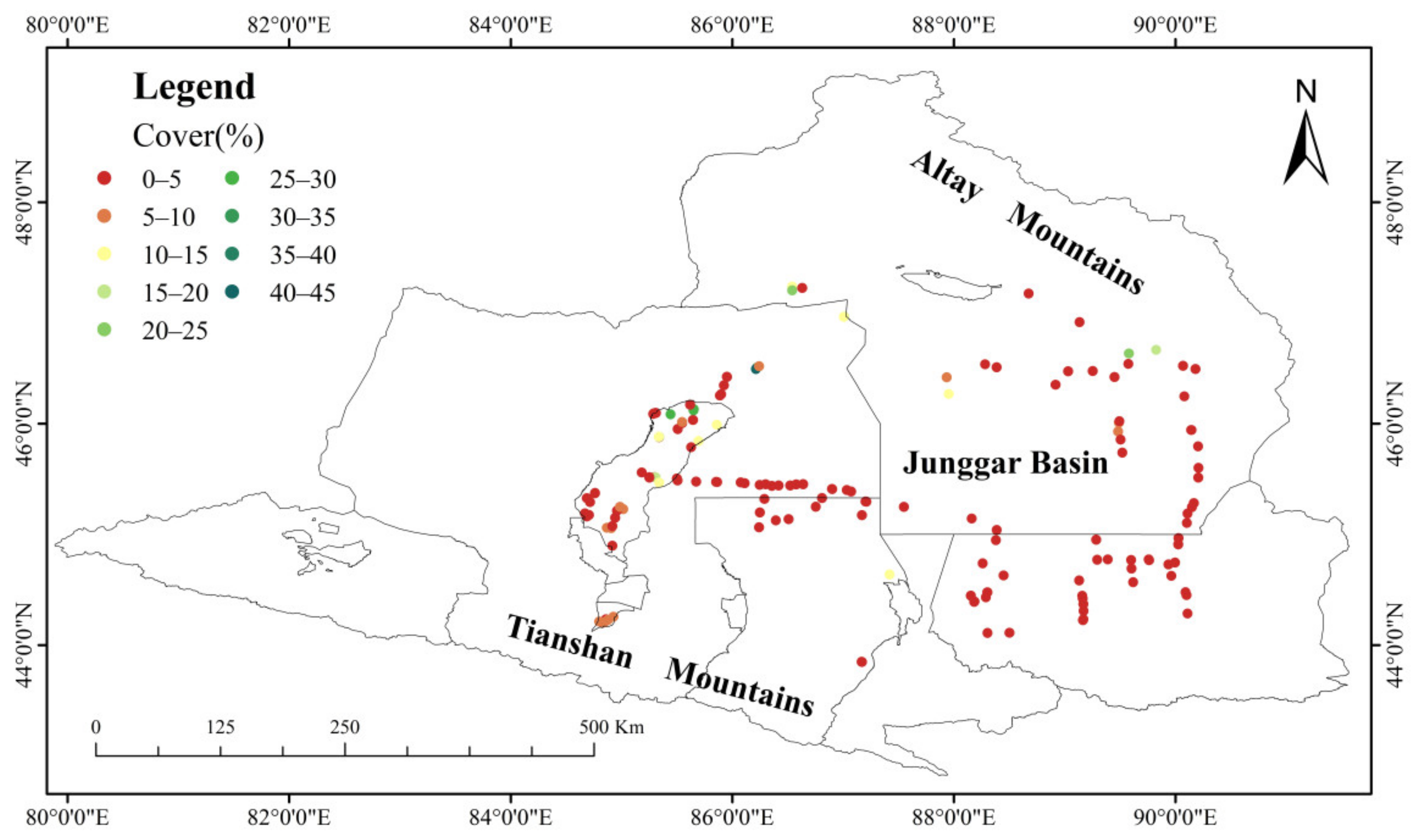
2.1. Study Area

The Junggar Basin is located in the north of the Uygur Autonomous Region, Xinjiang, China [42]. It is the second largest inland basin in China and is located between the Tianshan Mountains and the Altay Mountains [43], with a roughly triangular shape and an approximate range of 43–49°N and 80–91°E (Figure 1). In the basin, the Gurbantonggut Desert is the largest fixed or semifixed desert in China. The basin has a moderately temperate climate and is characterized by aridity, heat, sand, and a fragile ecological environment. The average elevation of the Junggar Basin is approximately 600 m, and the multiyear average temperature is 1.3–9.8 °C. The multiyear average precipitation in the basin is low, and the annual average precipitation does not exceed 150 mm. The average precipitation of the desert area in the center of the basin is only 70–100 mm, with an annual evaporation of up to 2000 mm [44]. The vegetation in the basin is sparse, and the species richness is low. The main plant species include Chenopodiaceae, Tamaricaceae, Asteraceae, and Leguminosae, and ultra-arid semi-trees, semi-shrubs, and shrubs or dry succulent plants predominate. The desert vegetation in the Junggar Basin plays an irreplaceable role in wind prevention, sand fixation, soil water conservation, water conservation, biodiversity protection, and regulation and stabilization of the temperature in the desert area [45].

2.2. Acquisition of Vegetation Coverage Field Data

The UAV was used to collect field survey data of the vegetation coverage in the peak growing season (from June to September) from 2019 to 2021 and to select the typical vegetation community with a uniform vegetation species distribution and growth state as the sample plot, with a size of 250 m × 250 m. The center of the sample plots coincided with the center of the MODIS data pixels. The field sample plots were arranged in the form of the Chinese character “井” to ensure uniform sampling in the Junggar Basin. The longitude, latitude, elevation, grassland type, and dominant species of each plot were recorded. According to the Map of Chinese Grassland Resources (Natural Resources Comprehensive Survey Commission, Chinese Academy of Sciences) [46], nine grassland types were identified in the study area, and the grassland types with a ratio of more than 1% to the study area were all assigned plots. For details, refer to Table 1. The longitude, latitude, altitude, grassland type, and dominant species of each sample plot were recorded. From 2019 to 2021, a total of 171 sample plots were included (66 in 2019, 28 in 2020, and 77 in 2021). The UAV used in this study was the DJI Mavic 2 Zoom-Drone Quadcopter UAV with an Optical Zoom Camera. The positioning accuracy of this UAV is ±1.5 m horizontally and ±0.5 m vertically. The 1/2.3″ CMOS Sensor has an effective pixel size of 12 million and a maximum photograph size of 4000 × 3000. When carrying out aerial field photography, the time period of 11:00–16:00 with clear weather and sufficient light was selected. Before each UAV flight, the white balance of the UAV camera was adjusted to ensure that high-quality UAV photographs were obtained. The flight speed of the UAV was 6 m/s (3 m/s when there was wind). The flight path of the UAV used the FragMAP aerial photography system [47]. The flight altitude was approximately 20 m, and 16 photographs were taken in each sample plot (250 m × 250 m).

2.3. UAV Aerial Photography Data Processing and Data Analysis

The photographs taken by the UAV were processed by Pixel Classifier software [48]. The vegetation coverage of each photograph was extracted using Pixel Classifier software, and the average vegetation coverage of the 16 photographs was taken as the true vegetation coverage of the sample plot. Pixel Classifier software divides each pixel in a photograph into bare land and vegetation by specifying a threshold. According to the enhanced greening index (EGI), the threshold is adjusted to the optimal threshold, which represents the vegetation coverage of the photo. The generated vegetation coverage is much better than that of the traditional five-point sampling method and is very close to the real coverage of the entire sample plot [48].

2.4. MODIS Data and Processing

The MODIS data were selected from the MODIS daily surface reflectance product (MOD09GA) of the United States National Aeronautics and Space Administration (NASA) for the 2000–2021 period and orbital numbers of h23v04 and h24v04. These data can be downloaded from the LAADS DAAC (https://ladsweb.modaps.eosdis.nasa.gov/search/, accessed on 18 December 2021). All images were processed according to the following steps: (1) The MOD09GA and MOD09GQ data were converted to GeoTIFF format and WGS84 geographic projection using the MODIS Reprojection Tool released by NASA, and then the surface spectral reflectance of bands 1–7 was extracted. (2) GS image fusion was performed on the MOD09GA and MOD09GQ data in the ENVI software to generate MOD09GA_GQ. (3) ArcGIS was used to extract the pixel values corresponding to the field measured plots in the red band, near-infrared band, and blue wave segment data of the new fused product MOD09GA_GQ (2019–2021). According to the formula, the NDVI, EVI, SAVI, OSAVI, and MSAVI were calculated. The calculation formula is shown in Table 2.

2.5. Environmental Factors and Pretreatment

The v4 Version 1 SRTM digital elevation model (DEM) data from the Geospatial Data Cloud, download address (http://www.gscloud.cn/home, accessed on 20 December 2021), were used in this study. The spatial resolution was 90 m, and the format was GeoTIFF. In total, six data scenes, with track numbers of 53-03, 53-04, 54-03, 54-04, 55-03, and 55-04, were required for the Junggar Basin. To match the spatial resolution of the MOD09GA_GQ data, the DEM data were resampled from a spatial resolution of 90 m to one of 250 m, and ArcGIS software was used to extract the longitude, latitude, aspect, slope, and elevation of each pixel within the study area.
The meteorological data were from the National Earth System Science Data Center, National Science & Technology Infrastructure of China (http://www.geodata.cn, accessed on 5 March 2022), and the product with interpolated monthly data was used to extract the temperature and precipitation of the grids corresponding to the field survey sample plots in ArcGIS. Due to the cumulative effect of climatic factors, in addition to the current climatic conditions that may affect vegetation growth, previous climatic conditions also affect vegetation growth [54]. Therefore, in this study, the monthly climatic factors were extracted several months before the field survey. The linear regression relationships between the collected field vegetation coverage in the current month and the average temperature and cumulative precipitation in the current month, in the previous month, in the second-to-last month…, and in the fifth-to-last month were obtained. The meteorological factors in the month with the strongest correlation were selected to establish the vegetation coverage model.

2.6. Establish and Evaluate the Inversion Model of Vegetation Coverage

The vegetation coverage inversion models included the multivariate parametric regression model, the SVM regression model, and the back-propagation neural network (BPNN) regression model. In MATLAB, the data of 171 plots were randomly divided into two parts at a ratio of 70:30. The extracted training set data were used to establish the multivariate regression model, the SVM regression model, and the BPNN regression model; the other test set data were used to verify the accuracy of all models.

2.6.1. Screening of Vegetation Coverage Sensitivity Indicators

We screened the relevant factors for the multivariate regression model, including the geographical location and topography (longitude, latitude, elevation, slope, aspect), meteorology (average temperature, cumulative precipitation), and vegetation indices (NDVI, EVI, SAVI, OSAVI, MSAVI). Factors, i.e., vegetation indices and environmental characteristics with a high correlation with vegetation coverage and passing the F test, were used to construct the models (including the multivariate regression model, the SVM regression model, and the BPNN regression model).

2.6.2. Establishment of the Vegetation Coverage Inversion Model

(1) The factors that were significantly correlated with vegetation coverage were selected as independent variables, and linear, exponential, and logarithmic regression models were constructed in SPSS 26 (Equations (1)–(3)):
y = β 0 + β 1 x 1 + β 2 x 2 + + β i x i + ε
y = β 0 e β 1 x 1 e β 2 x 2 e β i x i e ε
y = β 0 + β 1 lnx 1 + β 2 lnx 2 + + β i lnx i + ε
where y is the vegetation coverage; x 1 ,   x 2   ,   x i are the selected independent variables; β 0 ,   β 1 ,   β 2 ,   β I are the parameters representing the model; and ε represents the error term.
(2) The SVM regression model is a machine learning method commonly used to solve nonlinear regression estimation problems [55]. The SVM model is not sensitive to the sample size of the training set. Compared with other machine learning methods, the SVM model can achieve considerable accuracy with a small training sample size [56]. The factors with a significant correlation with vegetation coverage were selected as the model input, and the vegetation coverage extracted from the UAV images was selected as the model output to establish the SVM model. SVM regression was completed using the “LIBSVM” package in MATLAB (R2019b).
(3) The BPNN model is a popular neural network that can effectively estimate surface vegetation variables [57]. Therefore, the BPNN model was selected to compare the performance of the methods. In this study, the Levenberg–Marquardt algorithm was selected for training the model, the input and output of the model were consistent with those of the SVM model, and the number of nodes in the hidden layer was four. The establishment and validation of the BPNN model were performed using the neural network toolbox in MATLAB (R2019b).

2.7. Model Evaluation Indicators

R2 and mean squared error (MSE) were selected as the basis for evaluating the accuracy of the model. The formulas for R2 and MSE are as follows:
R 2 = SSE SST = 1 SSR SST
SSR = i = 1 n   cover   i f cover   i 2
SST = i = 1 n f cover   i cover ¯ 2
MSE = 1 n i = 1 n cover i f cover   i 2
where SSR is the sum of squares due to regression, SST is the total sum of squares,   cover i represents the ith field survey vegetation coverage, cover ¯ represents the average field survey vegetation coverage, f cover   i   represents the ith vegetation coverage estimated by the model and n represents the number of test sets.

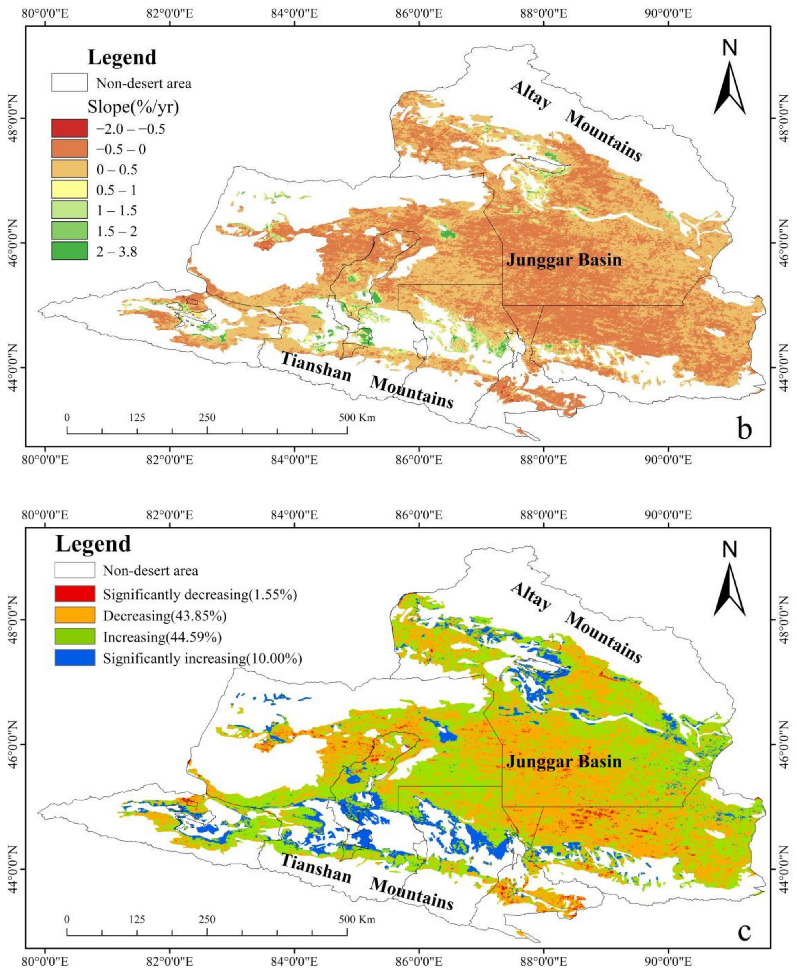
2.8. Spatial Distribution and Dynamic Changes in Vegetation Coverage

Using the optimal model and the dataset required by the optimal model, the yearly maximum vegetation coverage (i.e., July–September coverage) in the study area from 2000 to 2021 was determined using MATLAB software. After averaging these vegetation coverage datasets, the spatial distribution map of 22 years of average annual maximum vegetation coverage in the Junggar Basin was obtained.
The temporal variation in the maximum vegetation coverage from 2000 to 2021 was analyzed using the slope linear trend model. The model has the characteristics of simplicity and stability [58]. The model can simulate the change in vegetation coverage of each pixel to extrapolate the change in the entire study area [59]. To further analyze the importance of changes in the vegetation cover over time, we introduced the F-test [60]. By superimposing the slope and F test datasets, the changes in the vegetation cover for the entire study area were divided into four categories: significant increase (slope > 0%/yr and F > 4.60), increase (slope > 0%/yr and f < 4.60), decrease (slope < 0%/yr and f < 4.60), and significant decrease (slope < 0%/yr and F > 4.60) [61]. The slope equation is as follows:
slope   = n × i = 1 n i ×   cover   i i = 1 n i i = 1 n   cover   i n × i = 1 n i 2 i = 1 n i 2
where n is the total number of years (22); i is a number from 1–22, representing the year from 2000 to 2021; and   cover i is the annual maximum vegetation coverage stimulated by the selected optimal model in year i:
F = R 2 m 2 1 R 2
r = i = 1 m i   i ¯   cover   i cover ¯ i = 1 m ( i   i   ¯ ) 2 i = 1 m   cover   i cover ¯ 2
where m is equal to the total number of years (22); R 2 is the square of the correlation coefficient (r) between the coverage in each pixel and the time series; i ¯ is the average of the numbers 1–22, which is equal to 11.5;   cover   i is the annual maximum vegetation coverage simulated by the optimal model in year i; and cover ¯ is the annual average maximum vegetation coverage from 2000 to 2021.

3. Results

3.1. Spatial Distribution of Vegetation Coverage in Sample Plots Obtained from UAV Aerial Photography in 2019–2021

From 2019 to 2021, a total of 171 field sample plots were surveyed by UAVs. The spatial distribution and vegetation coverage of each sample plot are shown in Figure 2. The vegetation coverage of the sample plots was between 0% and 45%, and the average vegetation coverage of the sample plots was approximately 4%. Areas with a vegetation coverage of 0–5%, 5–10%, and >10% accounted for 80%, 10%, and 10% of the study area, respectively. The overall trend of vegetation coverage in the sample plots gradually decreased from north to south and from west to east. The sample plots collected near the Altay Mountains in the northwest and northeast of the Junggar Basin showed a relatively high vegetation coverage (>5%).

3.2. Correlations of Vegetation Coverage before and after GS Image Fusion

The MOD09GA_GQ data generated by fusing the 2019–2021 MOD09GA and MOD09GQ data of the study area using the GS sharpening method were used to calculate five vegetation indexes, including the NDVI, EVI, SAVI, OSAVI, and MSAVI, for the 171 sample plots, and the relationship of each vegetation index with the corresponding vegetation coverage obtained by the UAV aerial photography was analyzed. The results show that the correlations between the five vegetation indices obtained from the MOD09GA_GQ data and the vegetation coverage of the sample plots were all higher than those obtained directly from the MOD09GA data (Table 3), and the correlation between the MOD09GA_GQ EVI and the vegetation coverage was the highest (r = 0.72, p < 0.001), followed by SAVI (r = 0.71, p < 0.001), OSAVI (r = 0.70, p < 0.001), MSAVI (r = 0.70, p < 0.001), and NDVI (r = 0.69, p < 0.001), indicating that the MOD09GA_GQ EVI generated by the GS sharpening method is the optimal vegetation index for the inversion of the vegetation coverage of the Junggar Basin.

3.3. Results of Screening of Vegetation Coverage Sensitivity Indicators

In terms of the geographical location and topographic factors, the vegetation coverage showed the highest correlation with the longitude (r = −0.17, p < 0.05) and latitude of the observation site (r = 0.36, p < 0.001). The elevation, slope, and aspect were not significantly correlated with the vegetation coverage. In terms of the climatic factors, because vegetation growth often lags behind the variation in climatic factors [62], climate changes in the month of the field survey were not the factors with the strongest correlation with the vegetation coverage. An analysis of the climatic factors and vegetation coverage indicated that the correlation between the vegetation coverage of the current month and the average temperature of the previous month was the strongest (r = −0.27), reaching an extremely significant level (p < 0.001) (Table 4). The correlations between the vegetation coverage and the precipitation in the current month, previous month, and second-to-last month reached an extremely significant level, but the correlation with the precipitation in the previous month was the highest (r = 0.33, p < 0.001).
Therefore, the indicators that were most closely correlated were the MOD09GA_GQ EVI (r = 0.72, p < 0.001) (Table 3), longitude (r = −0.17, p < 0.05) (Table 4), latitude (r = 0.36, p < 0.001) (Table 4), cumulative precipitation of the current and previous months (r = 0.33, p < 0.001) (Table 4), and the average temperature of the current and previous months (Table 4). Therefore, five factors, i.e., the EVI, longitude, latitude, average temperature of the current and previous months, and cumulative precipitation of the current and previous months, were used as sensitive indicators of the vegetation coverage to construct an inversion model of vegetation cover in the Junggar Basin.

3.4. Evaluation of the Multivariate Parametric Regression Models

Table 5 assesses the accuracy of the multivariate parametric regression models based on the EVI, longitude, latitude, average temperature of the current and previous months, and the cumulative precipitation of the current and previous months. Among the three multivariate regression models, the multivariate linear model performed the best (R2 = 0.64, MSE = 9.11%). The power model (R2 = 0.51, MSE = 11.15%) showed a good performance. The logarithmic model (R2 = 0.47, MSE = 17.45%) performed the worst (Table 5). Therefore, the multivariate linear model can simulate the vegetation coverage in the Junggar Basin well, and its formula is shown in Table 6.

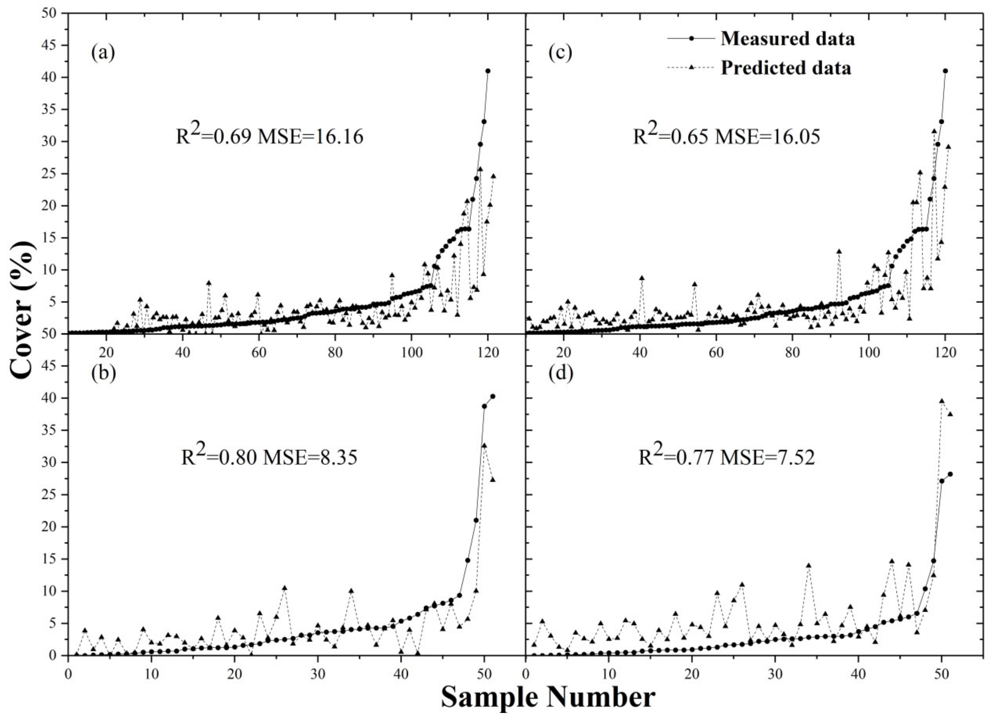
3.5. Accuracy Evaluation of the Multivariate Regression Models Based on the SVM and BPNN

Table 6 lists the accuracy evaluation results of the SVM and BPNN regression models. The SVM regression model performed better (R2 = 0.80, MSE = 8.35%) (Figure 3b). The BPNN regression model found R2 = 0.77 and MSE = 7.52% (Figure 3d). A comparison of Table 5 and Table 7 reveals that the SVM and BPNN regression models were significantly better than the linear nonlinear regression model based on multiple factors in the inversion of the low vegetation coverage in the desert area of the Junggar Basin. Therefore, the SVM regression model best simulated the vegetation coverage in the Junggar Basin. The details of the SVM model are given in Table 8.

3.6. Comparative Analysis of the Multivariate Parametric Regression Models and Machine Learning Regression Models

This study established multivariate parametric regression models (linear, logarithmic, and exponential), an SVM regression model, and a BPNN regression model based on UAV field vegetation coverage data, geographic location, terrain, meteorological data, and vegetation indices. Large differences were observed in the stability and accuracy of the models. In general, compared with the multifactor parametric model, the machine learning models (the SVM regression model and the BPNN regression model) showed better accuracy and stability values, and the R2 value increased by 0.13–0.33. Although the machine learning model was more accurate than the parametric regression model in the inversion of the vegetation coverage, the machine learning regression models have some shortcomings. For example, the BPNN model often has an overfitting problem. For the SVM model, the choice of the kernel function affects the analysis results, but choosing the optimal kernel function is difficult in practice. At present, the most suitable kernel function can only be selected based on previous experience and personal debugging in practice. In addition, because the SVM model depends on the support vector, not all training samples can be used (as a support vector). Therefore, as the number of samples increases and deep learning technology matures, other algorithmic models can be explored to more accurately estimate the vegetation coverage.

3.7. Analysis of the Spatial Distribution and Trend of Vegetation Coverage

In this study, the longitude, latitude, average temperature, cumulative precipitation, and EVI were selected, and the SVM regression method (best model) was used for the inversion of the yearly maximum vegetation coverage (i.e., the maximum coverage in July–September) in the study area for 22 years (2000–2021) using MATLAB software. Figure 4 shows the spatial distribution of the average yearly maximum vegetation coverage over the 22 years. The vegetation coverage in the Junggar Basin was between 0 and 67.44%, with an average coverage of 7.36%. The vegetation coverage in the northern and western regions of the Junggar Basin was relatively high, while that in the center of the basin was relatively low. Overall, the spatial distribution of the average yearly maximum vegetation coverage in the basin gradually decreased from the north and south sides to the center and from west to east.
In the past 22 years, the change trend of vegetation coverage in the desert of the Junggar Basin has mainly been concentrated around −0.5–0.5%/yr (Figure 5b), and the regions with a change trend above 0.5%/yr are distributed near the Tianshan and Altay Mountains. As shown in Figure 5c, the annual maximum vegetation coverage in 44.59% of the desert area in the Junggar Basin has increased, and the significantly increased area accounts for 10.00% of the desert area. Only 43.85% of the desert area of the basin has shown a decrease in vegetation coverage, of which 1.55% was significantly reduced (Figure 5c). These areas essentially coincide with the distribution of the areas of low vegetation coverage (Figure 4). Overall, from 2000 to 2021, the vegetation coverage in the study area increased.
From 2000 to 2021, the variation of average temperature and accumulated precipitation in the desert area of Junggar Basin was little. The average temperature in the desert area of Junggar Basin over 22 years showed an increasing trend, while the accumulated precipitation showed a decreasing trend. The regions where the average temperature showed an increasing trend were mainly distributed in the middle and west of the study area, and the average temperature in the east of the study area showed a decreasing trend (Figure 6a). The change in cumulative precipitation in the study area was quite different from the change in average temperature (Figure 6b). The cumulative precipitation in the west, east, south, and north of the study area near the Altay Mountains showed an increasing trend, while the cumulative precipitation in the middle and south of the study area near the Tianshan Mountains showed a decreasing trend. Figure 5c also showed that the areas with increasing vegetation coverage in the study area are mainly distributed in the east, west, and near the Tianshan Mountains and Altay Mountains in the north and south. Simultaneously, the cumulative precipitation in these areas showed an increasing trend, while the average temperature showed a decreasing trend. This is consistent with the results in Table 4 and Figure 6. The vegetation coverage in the desert area of Junggar Basin was positively correlated with the accumulated precipitation and negatively correlated with the average temperature. For the impact on the desert vegetation growth, the accumulated precipitation had higher influence than the average temperature (r = 0.33, F = 21.304 **, r = −0.27, F = 12.778 **, respectively).

4. Discussion

4.1. Comparison of the Applicability of the Five Vegetation Indices in Modeling the Vegetation Coverage

The vegetation indices that are commonly used to study the vegetation coverage include the NDVI, EVI, SAVI, OSAVI, and MSAVI [63]. The NDVI is currently the most widely used vegetation index, and it has been used in the inversion of vegetation dynamics in many studies [42]. To eliminate the influence of the soil background, the SAVI and MSAVI were improved from the NDVI by Qi et al. [53] and Huete [51], respectively, but these indices are not superior to the NDVI in terms of quantifying the vegetation coverage in arid environments [64,65]. The EVI is more suitable for areas with a high biomass than the NDVI [66]. We found that the EVI performed better than the NDVI in the arid region, similar to the results of Evrendilek and Gulbeyaz [18], who proposed that the EVI could better reflect the vegetation coverage in the arid and semiarid regions of Asia. In desert areas, the NDVI is more susceptible to the spectral effects of the soil texture, moisture, atmosphere, and other factors compared to the EVI [67]. Therefore, when constructing the vegetation coverage model in the desert area of the Junggar Basin, the EVI is the optimal vegetation index.

4.2. Advantages, Disadvantages, and Future Prospects of Image Fusion

In this study, MOD09GA and MOD09GQ data were fused using the GS sharpening method, and the results show that the spatial mismatch between the measured data and the remote sensing data was effectively solved by image fusion [68]. In contrast to this study, most image fusion studies in the field of ecology have focused on the fusion of high-precision remote sensing images. Quan et al. [69] fused GF-3 and Sentinel-2A images to obtain products with a spatial resolution of 10 m for land classification, and the results indicated that image fusion has the potential to improve the accuracy of land cover classification by remote sensing data. Dao et al. [70] used the ESTARFM method to fuse Landsat and MODIS data to generate data with a spatial resolution of 30 m to study flood inundation, and they found that the image fusion technique was useful for the observation of flood inundation in vegetated areas. To obtain remote sensing data with high spatial and temporal resolutions, remote sensing data from two different remote sensing image sources, such as MODIS and Landsat, and GF-3 and Sentinel-2A, are usually required; however, each remote sensing image source has its own specifications, such as the orbital altitude, band limits, and relative spectral response of the sensor, which can introduce new errors in the fusion process [71,72]. The MOD09GA and MOD09GQ data used in this study were both from the MODIS sensor onboard the Terra satellite; therefore, errors caused by the sensors were avoided. The accuracy of the vegetation index estimation generally tends to decrease as the pixel size of the remote sensing data increases [68], and fusing the remote sensing data from two remote sensing sources is consequently still necessary to improve the accuracy. Therefore, in future studies, we will focus on producing large-area, high-precision, and full-band remote sensing products with reduced sensor errors using image fusion.

4.3. Factors Affecting the Accuracy of the Optimal Vegetation Coverage Inversion Model

Compared with the other models in this study, the SVM regression model showed higher stability and a better prediction ability, but problems remain due to the limitations of various factors.
First, due to the sparse vegetation in the Junggar Basin, the bare soil background could have caused interference with the spectral characteristics of the vegetation [73]. In addition, moderate-resolution (250 m) remote sensing images were used in this study, and the corresponding spectral bands extracted from the remote sensing images had a low accuracy [74]; therefore, the calculated vegetation indices could have underestimated the actual vegetation coverage of the study area, resulting in inaccurate inversion by the model. Even if the sample plot is located in an area with uniform vegetation during field sampling, these errors will still affect the accuracy of the model.
The choice of factors for establishing the model will also affect the prediction accuracy of the model [23,75]. Yang et al. [22] found that the vegetation coverage was correlated with biomass and height. However, in the desert area of the Junggar Basin, vegetation is extremely scarce, and the average height of the vegetation in some areas is above 5 m, which makes it difficult to measure. In the desert area of the basin, obtaining aboveground biomass by logging is forbidden, and the data obtained by other means are inaccurate [76]. Therefore, in this study, factors (such as the geographical location, topography, meteorological data, and vegetation index) that are easy to obtain and do not affect the ecological environment were used to build the model.

4.4. Trend of Vegetation Coverage and Possible Causes

Climate change is an important factor that can lead to changes in the vegetation coverage in arid areas. Liu et al. [2] showed that changes in the vegetation coverage in arid areas are affected by the combined or synergistic effects of the comprehensive or synergistic effects of climate conditions such as the temperature, precipitation, and humidity. This study analyzed the relationships of the vegetation coverage with the temperature and precipitation in 2019–2021 and found that the vegetation coverage in the Junggar Basin was positively correlated with precipitation and negatively correlated with temperature. In the past few decades, Xinjiang has experienced simultaneous increases in temperature and precipitation [77]. The vegetation coverage in the desert area of the Junggar Basin in Xinjiang has obviously increased, which shows that the positive impact of precipitation on the vegetation coverage in the desert area of Junggar Basin is higher than the negative impact of temperature, which is consistent with the research of Xue et al. [78]
Of course, human activities can also lead to changes in the vegetation coverage. Human activities can help restore vegetation to previous ecological levels [79]. Zhang et al. [80] demonstrated that most of the increase in grassland productivity in Xinjiang from 2000 to 2014 came from human intervention. The increase in the vegetation coverage in the desert area of the Junggar Basin may be related to the grassland protection projects launched in recent years [81]. We believe that vegetation protection projects in the desert area have played an important role in increasing the coverage of desert vegetation. We should continue to maintain corresponding policies and promote the development of desert vegetation.

5. Conclusions

This study used the UAV-measured vegetation coverage data of the Junggar Basin from 2019 to 2021, downloaded and preprocessed the MODIS VI product, analyzed the influencing factors of the vegetation coverage in the Junggar Basin, constructed three types of inversion models for vegetation coverage, and evaluated the accuracy and stability of the models. The following conclusions can be drawn.
(1) The daily full-band product MOD09GA_GQ with a spatial resolution of 250 m was obtained by processing MOD09GA and MOD09GQ data through GS fusion, which improved the correlation between the vegetation coverage extracted from the UAV images and the vegetation indices obtained from the remote sensing data. This result indicates that image fusion can solve the problem of spatial matching between remote sensing data and UAV images.
(2) Five vegetation indices, the NDVI, EVI, SAVI, OSAVI, and MSAVI, were highly significantly correlated with the vegetation coverage (p < 0.001). The EVI had the strongest correlation (r = 0.72, p < 0.001). Considering only the geographic and topographic variables, the vegetation coverage had the strongest correlation with the longitude (r = −0.17, p < 0.05) and latitude (r = 0.36, p < 0.001); based on the meteorological factors, the vegetation coverage had the strongest correlation with the cumulative precipitation in the current and previous months (r = 0.33, p < 0.001) and the average temperature in the current and previous months (r = −0.27, p < 0.001).
(3) Based on the EVI, longitude, latitude, cumulative precipitation of the current and previous months, and the average temperature of the current and previous months, we built a multiple factor linear regression model (R2 = 0.64, MSE = 9.11%), an SVM regression model (R2 = 0.80, MSE = 8.35%), and a BPNN regression model (R2 = 0.77, MSE = 7.52%), and they all performed well when inverting the vegetation coverage of the Junggar Basin. The SVM regression model had the highest accuracy.
(4) From 2000 to 2021, the average yearly maximum vegetation coverage in the desert area of the Junggar Basin was 7.36%, and the vegetation coverage in the Junggar Basin gradually decreased from the north and south sides to the center and from west to east. In the past 22 years, the vegetation coverage in 54.59% of the Junggar Basin increased.

Author Contributions

All authors contributed significantly to this manuscript. To be specific, Y.M. and R.Z. designed this study. Y.M. wrote the main manuscript text. J.G., J.L. and Y.M. conducted field surveys. Y.M. and S.Y. analyzed the data and prepared figures. B.M. helped in interpreting the results and editing the language. All authors have read and agreed to the published version of the manuscript.

Funding

This research was supported by the National Natural Science Foundation of China (31860145), Special Funds of The Central Government (Xin [2020]TG06), and Talent Introduction Project of Xinjiang University (2020BS05).

Data Availability Statement

The MODIS data can be downloaded from the LAADS DAAC (https://ladsweb.modaps.eosdis.nasa.gov/search/, accessed on 18 December 2021); The DEM data were 90 m SRTM digital elevation model (DEM) data(v4 Version 1) from the Geospatial Data Cloud, download address (http://www.gscloud.cn/home, accessed on 20 December 2021); The meteorological data were from the National Earth System Science Data Center, National Science & Technology Infrastructure of China (http://www.geodata.cn, accessed on 5 March 2022).

Acknowledgments

Acknowledgement for the data support from “National Earth System Science Data Center, National Science & Technology Infrastructure of China. (http://www.geodata.cn)”. We also appreciate the editor’s and reviewers’ constructive suggestions to greatly improve the paper.

Conflicts of Interest

The authors declare no conflict of interest.

References

  1. Peng, J.; Liu, Z.; Liu, Y.; Wu, J.; Han, Y. Trend analysis of vegetation dynamics in Qinghai–Tibet Plateau using Hurst Exponent. Ecol. Indic. 2012, 14, 28–39. [Google Scholar] [CrossRef]
  2. Liu, Y.; Li, L.; Chen, X.; Zhang, R.; Yang, J. Temporal-spatial variations and influencing factors of vegetation cover in Xinjiang from 1982 to 2013 based on GIMMS-NDVI3g. Glob. Planet. Change 2018, 169, 145–155. [Google Scholar] [CrossRef]
  3. Rodríguez-Maturino, A.; Martínez-Guerrero, J.H.; Chairez-Hernández, I.; Pereda-Solis, M.E.; Villarreal-Guerrero, F.; Renteria-Villalobos, M.; Pinedo-Alvarez, A. Mapping land cover and estimating the grassland structure in a priority area of the Chihuahuan desert. Land 2017, 6, 70. [Google Scholar] [CrossRef] [Green Version]
  4. Yu, H.; Xu, J. Effects of climate change on vegetations on Qinghai-Tibet Plateau: A review. Chin. J. Ecol. 2009, 28, 747–754. [Google Scholar] [CrossRef]
  5. Gitelson, A.A.; Kaufman, Y.J.; Stark, R.; Rundquist, D. Novel algorithms for remote estimation of vegetation fraction. Remote Sens. Environ. 2002, 80, 76–87. [Google Scholar] [CrossRef] [Green Version]
  6. Wei, Q.; Qingke, Z.; Xuexia, Z. Review of vegetation covering and its measuring and calculating method. J. Northwest Sci.-Tech. Univ. Agric. For. 2006, 34, 163–170. [Google Scholar] [CrossRef]
  7. Wang, J.; Wang, K.; Zhang, M.; Zhang, C. Impacts of climate change and human activities on vegetation cover in hilly southern China. Ecol. Eng. 2015, 81, 451–461. [Google Scholar] [CrossRef]
  8. Xin, Z.; Xu, J.; Zheng, W. Spatiotemporal variations of vegetation cover on the Chinese Loess Plateau (1981–2006): Impacts of climate changes and human activities. Sci. China Ser. D Earth Sci. 2008, 51, 67–78. [Google Scholar] [CrossRef]
  9. Fang, S.; Yan, J.; Che, M.; Zhu, Y.; Liu, Z.; Pei, H.; Zhang, H.; Xu, G.; Lin, X. Climate change and the ecological responses in Xinjiang, China: Model simulations and data analyses. Quat. Int. 2013, 311, 108–116. [Google Scholar] [CrossRef]
  10. Yang, H.; Mu, S.; Li, J. Effects of ecological restoration projects on land use and land cover change and its influences on territorial NPP in Xinjiang, China. Catena 2014, 115, 85–95. [Google Scholar] [CrossRef]
  11. Curran, P.; Williamson, H. Sample size for ground and remotely sensed data. Remote Sens. Environ. 1986, 20, 31–41. [Google Scholar] [CrossRef]
  12. Jia, K.; Liang, S.; Gu, X.; Baret, F.; Wei, X.; Wang, X.; Yao, Y.; Yang, L.; Li, Y. Fractional vegetation cover estimation algorithm for Chinese GF-1 wide field view data. Remote Sens. Environ. 2016, 177, 184–191. [Google Scholar] [CrossRef]
  13. Townshend, J.R.; Justice, C. Analysis of the dynamics of African vegetation using the normalized difference vegetation index. Int. J. Remote Sens. 1986, 7, 1435–1445. [Google Scholar] [CrossRef]
  14. Barati, S.; Rayegani, B.; Saati, M.; Sharifi, A.; Nasri, M. Comparison the accuracies of different spectral indices for estimation of vegetation cover fraction in sparse vegetated areas. Egypt. J. Remote Sens. Space Sci. 2011, 14, 49–56. [Google Scholar] [CrossRef] [Green Version]
  15. Yang, J.; Weisberg, P.J.; Bristow, N.A. Landsat remote sensing approaches for monitoring long-term tree cover dynamics in semi-arid woodlands: Comparison of vegetation indices and spectral mixture analysis. Remote Sens. Environ. 2012, 119, 62–71. [Google Scholar] [CrossRef]
  16. Zeng, L.; Wardlow, B.D.; Hu, S.; Zhang, X.; Zhou, G.; Peng, G.; Xiang, D.; Wang, R.; Meng, R.; Wu, W. A novel strategy to reconstruct NDVI time-series with high temporal resolution from MODIS multi-temporal composite products. Remote Sens. 2021, 13, 1397. [Google Scholar] [CrossRef]
  17. Li, Z.; Li, X.; Wei, D.; Xu, X.; Wang, H. An assessment of correlation on MODIS-NDVI and EVI with natural vegetation coverage in Northern Hebei Province, China. Procedia Environ. Sci. 2010, 2, 964–969. [Google Scholar] [CrossRef] [Green Version]
  18. Evrendilek, F.; Gulbeyaz, O. Deriving vegetation dynamics of natural terrestrial ecosystems from MODIS NDVI/EVI data over Turkey. Sensors 2008, 8, 5270–5302. [Google Scholar] [CrossRef] [Green Version]
  19. Ishiyama, T.; Nakajima, Y.; Kajiwara, K.; Tsuchiya, K. Extraction of vegetation cover in an arid area based on satellite data. Adv. Space Res. 1997, 19, 1375–1378. [Google Scholar] [CrossRef]
  20. Fern, R.R.; Foxley, E.A.; Bruno, A.; Morrison, M.L. Suitability of NDVI and OSAVI as estimators of green biomass and coverage in a semi-arid rangeland. Ecol. Indic. 2018, 94, 16–21. [Google Scholar] [CrossRef]
  21. Purevdorj, T.; Tateishi, R.; Ishiyama, T.; Honda, Y. Relationships between percent vegetation cover and vegetation indices. Int. J. Remote Sens. 1998, 19, 3519–3535. [Google Scholar] [CrossRef]
  22. Yang, S.; Feng, Q.; Liang, T.; Liu, B.; Zhang, W.; Xie, H. Modeling grassland above-ground biomass based on artificial neural network and remote sensing in the Three-River Headwaters Region. Remote Sens. Environ. 2018, 204, 448–455. [Google Scholar] [CrossRef]
  23. Ge, J.; Meng, B.; Liang, T.; Feng, Q.; Gao, J.; Yang, S.; Huang, X.; Xie, H. Modeling alpine grassland cover based on MODIS data and support vector machine regression in the headwater region of the Huanghe River, China. Remote Sens. Environ. 2018, 218, 162–173. [Google Scholar] [CrossRef]
  24. Meng, B.; Gao, J.; Liang, T.; Cui, X.; Ge, J.; Yin, J.; Feng, Q.; Xie, H. Modeling of alpine grassland cover based on unmanned aerial vehicle technology and multi-factor methods: A case study in the east of Tibetan Plateau, China. Remote Sens. 2018, 10, 320. [Google Scholar] [CrossRef] [Green Version]
  25. Lin, X.; Chen, J.; Lou, P.; Yi, S.; Qin, Y.; You, H.; Han, X. Improving the estimation of alpine grassland fractional vegetation cover using optimized algorithms and multi-dimensional features. Plant Methods 2021, 17, 96. [Google Scholar] [CrossRef] [PubMed]
  26. Hansen, M.; DeFries, R.; Townshend, J.; Sohlberg, R.; Dimiceli, C.; Carroll, M. Towards an operational MODIS continuous field of percent tree cover algorithm: Examples using AVHRR and MODIS data. Remote Sens. Environ. 2002, 83, 303–319. [Google Scholar] [CrossRef]
  27. Huang, C.; Song, K.; Kim, S.; Townshend, J.R.; Davis, P.; Masek, J.G.; Goward, S.N. Use of a dark object concept and support vector machines to automate forest cover change analysis. Remote Sens. Environ. 2008, 112, 970–985. [Google Scholar] [CrossRef]
  28. Yuan, Q.; Shen, H.; Li, T.; Li, Z.; Li, S.; Jiang, Y.; Xu, H.; Tan, W.; Yang, Q.; Wang, J. Deep learning in environmental remote sensing: Achievements and challenges. Remote Sens. Environ. 2020, 241, 111716. [Google Scholar] [CrossRef]
  29. Chen, J.; Yi, S.; Yu, Q.; Xiaoyun, W. Improving estimates of fractional vegetation cover based on UAV in alpine grassland on the Qinghai–Tibetan Plateau. Int. J. Remote Sens. 2016, 37, 1922–1936. [Google Scholar] [CrossRef]
  30. Zhang, H.; Sun, Y.; Chang, L.; Qin, Y.; Chen, J.; Qin, Y.; Du, J.; Yi, S.; Wang, Y. Estimation of grassland canopy height and aboveground biomass at the quadrat scale using unmanned aerial vehicle. Remote Sens. 2018, 10, 851. [Google Scholar] [CrossRef]
  31. Zhang, J.; Liu, D.; Meng, B.; Chen, J.; Wang, X.; Jiang, H.; Yu, Y.; Yi, S. Using UAVs to assess the relationship between alpine meadow bare patches and disturbance by pikas in the source region of Yellow River on the Qinghai-Tibetan Plateau. Glob. Ecol. Conserv. 2021, 26, e01517. [Google Scholar] [CrossRef]
  32. Zhang, X.; Yuan, Y.; Zhu, Z.; Ma, Q.; Yu, H.; Li, M.; Ma, J.; Yi, S.; He, X.; Sun, Y. Predicting the Distribution of Oxytropis ochrocephala Bunge in the Source Region of the Yellow River (China) Based on UAV Sampling Data and Species Distribution Model. Remote Sens. 2021, 13, 5129. [Google Scholar] [CrossRef]
  33. Kaivosoja, J.; Hautsalo, J.; Heikkinen, J.; Hiltunen, L.; Ruuttunen, P.; Näsi, R.; Niemeläinen, O.; Lemsalu, M.; Honkavaara, E.; Salonen, J. Reference measurements in developing UAV Systems for detecting pests, weeds, and diseases. Remote Sens. 2021, 13, 1238. [Google Scholar] [CrossRef]
  34. Abdollahnejad, A.; Panagiotidis, D.; Surový, P.; Modlinger, R. Investigating the Correlation between Multisource Remote Sensing Data for Predicting Potential Spread of Ips typographus L. Spots in Healthy Trees. Remote Sens. 2021, 13, 4953. [Google Scholar] [CrossRef]
  35. Xu, Q. Image Fusion and Stylization Processing Based on Multiscale Transformation and Convolutional Neural Network. Comput. Intell. Neurosci. 2022, 2022, 1181189. [Google Scholar] [CrossRef]
  36. Sales, M.H.R.; Souza, C.M.; Kyriakidis, P.C. Fusion of MODIS images using kriging with external drift. IEEE Trans. Geosci. Remote Sens. 2012, 51, 2250–2259. [Google Scholar] [CrossRef]
  37. Monsalve-Tellez, J.M.; Torres-León, J.L.; Garcés-Gómez, Y.A. Evaluation of SAR and Optical Image Fusion Methods in Oil Palm Crop Cover Classification Using the Random Forest Algorithm. Agriculture 2022, 12, 955. [Google Scholar] [CrossRef]
  38. Sarp, G. Spectral and spatial quality analysis of pan-sharpening algorithms: A case study in Istanbul. Eur. J. Remote Sens. 2014, 47, 19–28. [Google Scholar] [CrossRef] [Green Version]
  39. Liu, Q. Sharpening the WBSI imagery of Tiangong-II: Gram-Schmidt and principal components transform in comparison. In Proceedings of the 2018 14th International Conference on Natural Computation, Fuzzy Systems and Knowledge Discovery (ICNC-FSKD), Huangshan, China, 28–30 July 2018; pp. 511–518. [Google Scholar]
  40. Yang, J.; Ren, G.; Ma, Y.; Fan, Y. Coastal wetland classification based on high resolution SAR and optical image fusion. In Proceedings of the 2016 IEEE International Geoscience and Remote Sensing Symposium (IGARSS), Beijing, China, 10–15 July 2016; pp. 886–889. [Google Scholar]
  41. Hashim, F.; Dibs, H.; Jaber, H.S. Adopting Gram-Schmidt and Brovey Methods for Estimating Land Use and Land Cover Using Remote Sensing and Satellite Images. Nat. Environ. Pollut. Technol. 2022, 21, 867–881. [Google Scholar] [CrossRef]
  42. Cheng, D.; Ling, W.; Lingyun, H.; Shaoming, W. Spatio-temporal distribution pattern of vegetation coverage in Junggar Basin, Xinjiang. Acta Ecol. Sin. 2016, 36, 72–76. [Google Scholar] [CrossRef]
  43. Xie, C.; Wu, S.; Zhuang, Q.; Zhang, Z.; Hou, G.; Luo, G.; Hu, Z. Where Anthropogenic Activity Occurs, Anthropogenic Activity Dominates Vegetation Net Primary Productivity Change. Remote Sens. 2022, 14, 1092. [Google Scholar] [CrossRef]
  44. Jun, R.; Ling, T. Multivariate characterization of vegetation in Junnger basin. Acta Agrestia Sin. 2005, 13, 134–139. [Google Scholar] [CrossRef]
  45. Chang, Z.; Zhang, X.; Wang, Q.; Zhang, D.; Duan, X.; Shi, X. Temperature Regulation Effect of Desert Vegetation in Minqin Desert Area. Anim. Husb. Feed Sci. 2016, 8, 364–368. [Google Scholar] [CrossRef]
  46. Zhang, R.; Guo, J.; Yin, G. Response of net primary productivity to grassland phenological changes in Xinjiang, China. PeerJ 2021, 9, e10650. [Google Scholar] [CrossRef]
  47. Yi, S. FragMAP: A tool for long-term and cooperative monitoring and analysis of small-scale habitat fragmentation using an unmanned aerial vehicle. Int. J. Remote Sens. 2016, 38, 2686–2697. [Google Scholar] [CrossRef]
  48. Tang, L.; He, M.; Li, X. Verification of fractional vegetation coverage and NDVI of desert vegetation via UAVRS technology. Remote Sens. 2020, 12, 1742. [Google Scholar] [CrossRef]
  49. Tucker, C.J.; Sellers, P. Satellite remote sensing of primary production. Int. J. Remote Sens. 1986, 7, 1395–1416. [Google Scholar] [CrossRef] [Green Version]
  50. Huete, A.; Justice, C.; Liu, H. Development of vegetation and soil indices for MODIS-EOS. Remote Sens. Environ. 1994, 49, 224–234. [Google Scholar] [CrossRef]
  51. Huete, A.R. A soil-adjusted vegetation index (SAVI). Remote Sens. Environ. 1988, 25, 295–309. [Google Scholar] [CrossRef]
  52. Steven, M.D. The sensitivity of the OSAVI vegetation index to observational parameters. Remote Sens. Environ. 1998, 63, 49–60. [Google Scholar] [CrossRef]
  53. Qi, J.; Chehbouni, A.; Huete, A.R.; Kerr, Y.H.; Sorooshian, S. A modified soil adjusted vegetation index. Remote Sens. Environ. 1994, 48, 119–126. [Google Scholar] [CrossRef]
  54. Luo, N.; Mao, D.; Wen, B.; Liu, X. Climate change affected vegetation dynamics in the northern Xinjiang of China: Evaluation by SPEI and NDVI. Land 2020, 9, 90. [Google Scholar] [CrossRef] [Green Version]
  55. Yang, L.; Jia, K.; Liang, S.; Liu, J.; Wang, X. Comparison of four machine learning methods for generating the GLASS fractional vegetation cover product from MODIS data. Remote Sens. 2016, 8, 682. [Google Scholar] [CrossRef] [Green Version]
  56. Camps-Valls, G.; Bruzzone, L.; Rojo-Álvarez, J.L.; Melgani, F. Robust support vector regression for biophysical variable estimation from remotely sensed images. IEEE Geosci. Remote Sens. Lett. 2006, 3, 339–343. [Google Scholar] [CrossRef]
  57. Baret, F.; Weiss, M.; Lacaze, R.; Camacho, F.; Makhmara, H.; Pacholcyzk, P.; Smets, B. GEOV1: LAI and FAPAR essential climate variables and FCOVER global time series capitalizing over existing products. Part1: Principles of development and production. Remote Sens. Environ. 2013, 137, 299–309. [Google Scholar] [CrossRef]
  58. Fensholt, R.; Rasmussen, K.; Nielsen, T.T.; Mbow, C. Evaluation of earth observation based long term vegetation trends—Intercomparing NDVI time series trend analysis consistency of Sahel from AVHRR GIMMS, Terra MODIS and SPOT VGT data. Remote Sens. Environ. 2009, 113, 1886–1898. [Google Scholar] [CrossRef]
  59. Zhao, H.; Liu, S.; Dong, S.; Su, X.; Wang, X.; Wu, X.; Wu, L.; Zhang, X. Analysis of vegetation change associated with human disturbance using MODIS data on the rangelands of the Qinghai-Tibet Plateau. Rangel. J. 2015, 37, 77–87. [Google Scholar] [CrossRef]
  60. Song, Y.; Ma, M.; Veroustraete, F. Comparison and conversion of AVHRR GIMMS and SPOT VEGETATION NDVI data in China. Int. J. Remote Sens. 2010, 31, 2377–2392. [Google Scholar] [CrossRef]
  61. Lin, H.; Zhao, Y.; Kalhoro, G.M. Ecological Response of the Subsidy and Incentive System for Grassland Conservation in China. Land 2022, 11, 358. [Google Scholar] [CrossRef]
  62. Zhu, W.; Mao, F.; Xu, Y.; Zheng, J.; Song, L. Analysis on response of vegetation index to climate change and its prediction in the three-rivers-source region. Plateau Meteorol. 2019, 38, 693–704. [Google Scholar] [CrossRef]
  63. Zhang, C.; Lu, D.; Chen, X.; Zhang, Y.; Maisupova, B.; Tao, Y. The spatiotemporal patterns of vegetation coverage and biomass of the temperate deserts in Central Asia and their relationships with climate controls. Remote Sens. Environ. 2016, 175, 271–281. [Google Scholar] [CrossRef]
  64. Franklin, J.; Duncan, J.; Turner, D.L. Reflectance of vegetation and soil in Chihuahuan desert plant communities from ground radiometry using SPOT wavebands. Remote Sens. Environ. 1993, 46, 291–304. [Google Scholar] [CrossRef]
  65. McGwire, K.; Minor, T.; Fenstermaker, L. Hyperspectral mixture modeling for quantifying sparse vegetation cover in arid environments. Remote Sens. Environ. 2000, 72, 360–374. [Google Scholar] [CrossRef]
  66. Liu, B.; Shen, W.; Lin, N.; Li, R.; Yue, Y. Deriving vegetation fraction information for the alpine grassland on the Tibetan plateau using in situ spectral data. J. Appl. Remote Sens. 2014, 8, 083630. [Google Scholar] [CrossRef]
  67. Lu, L.; Kuenzer, C.; Wang, C.; Guo, H.; Li, Q. Evaluation of three MODIS-derived vegetation index time series for dryland vegetation dynamics monitoring. Remote Sens. 2015, 7, 7597–7614. [Google Scholar] [CrossRef] [Green Version]
  68. Yu, Y.; Pan, Y.; Yang, X.; Fan, W. Spatial Scale Effect and Correction of Forest Aboveground Biomass Estimation Using Remote Sensing. Remote Sens. 2022, 14, 2828. [Google Scholar] [CrossRef]
  69. Quan, Y.; Tong, Y.; Feng, W.; Dauphin, G.; Huang, W.; Xing, M. A novel image fusion method of multi-spectral and sar images for land cover classification. Remote Sens. 2020, 12, 3801. [Google Scholar] [CrossRef]
  70. Dao, P.D.; Mong, N.T.; Chan, H.-P. Landsat-MODIS image fusion and object-based image analysis for observing flood inundation in a heterogeneous vegetated scene. GIScience Remote Sens. 2019, 56, 1148–1169. [Google Scholar] [CrossRef]
  71. Cao, L.; Liu, T.; Wei, L. A comparison of multi-resource remote sensing data for vegetation indices. In Proceedings of the IOP Conference Series: Earth and Environmental Science, Beijing, China, 22–26 April 2013; p. 012067. [Google Scholar]
  72. Soudani, K.; François, C.; Le Maire, G.; Le Dantec, V.; Dufrêne, E. Comparative analysis of IKONOS, SPOT, and ETM+ data for leaf area index estimation in temperate coniferous and deciduous forest stands. Remote Sens. Environ. 2006, 102, 161–175. [Google Scholar] [CrossRef] [Green Version]
  73. Shi, Y.; Wang, Z.; Liu, L.; Li, C.; Peng, D.; Xiao, P. Improving Estimation of Woody Aboveground Biomass of Sparse Mixed Forest over Dryland Ecosystem by Combining Landsat-8, GaoFen-2, and UAV Imagery. Remote Sens. 2021, 13, 4859. [Google Scholar] [CrossRef]
  74. Tian, H.; Wang, Y.; Chen, T.; Zhang, L.; Qin, Y. Early-Season Mapping of Winter Crops Using Sentinel-2 Optical Imagery. Remote Sens. 2021, 13, 3822. [Google Scholar] [CrossRef]
  75. Wang, Y.; Zhang, Z.; Feng, L.; Du, Q.; Runge, T. Combining multi-source data and machine learning approaches to predict winter wheat yield in the conterminous United States. Remote Sens. 2020, 12, 1232. [Google Scholar] [CrossRef] [Green Version]
  76. Morais, T.G.; Teixeira, R.F.; Figueiredo, M.; Domingos, T. The use of machine learning methods to estimate aboveground biomass of grasslands: A review. Ecol. Indic. 2021, 130, 108081. [Google Scholar] [CrossRef]
  77. Xiao, J.; Eziz, A.; Zhang, H.; Wang, Z.; Tang, Z.; Fang, J. Responses of four dominant dryland plant species to climate change in the Junggar Basin, northwest China. Ecol. Evol. 2019, 9, 13596–13607. [Google Scholar] [CrossRef]
  78. Xue, J.; Wang, Y.; Teng, H.; Wang, N.; Li, D.; Peng, J.; Biswas, A.; Shi, Z. Dynamics of Vegetation Greenness and Its Response to Climate Change in Xinjiang over the Past Two Decades. Remote Sens. 2021, 13, 4063. [Google Scholar] [CrossRef]
  79. Yin, F.; Deng, X.; Jin, Q.; Yuan, Y.; Zhao, C. The impacts of climate change and human activities on grassland productivity in Qinghai Province, China. Front. Earth Sci. 2014, 8, 93–103. [Google Scholar] [CrossRef]
  80. Zhang, R.; Liang, T.; Guo, J.; Xie, H.; Feng, Q.; Aimaiti, Y. Grassland dynamics in response to climate change and human activities in Xinjiang from 2000 to 2014. Sci. Rep. 2018, 8, 2888. [Google Scholar] [CrossRef] [PubMed] [Green Version]
  81. Xue, J.; Gui, D.; Lei, J.; Sun, H.; Zeng, F.; Mao, D.; Jin, Q.; Liu, Y. Oasification: An unable evasive process in fighting against desertification for the sustainable development of arid and semiarid regions of China. Catena 2019, 179, 197–209. [Google Scholar] [CrossRef]
Figure 1. Location of sample plots for vegetation coverage in the Junggar Basin (obtained by UAV) in 2019–2021.
Remotesensing 14 05146 g001
Figure 2. Spatial distribution of vegetation coverage in the sample plots taken by UAVs from 2019–2021 (n = 171).
Remotesensing 14 05146 g002
Figure 3. Relationships between the estimated and measured vegetation coverages in the training set (a) and test set (b) by the SVM regression model and in the training set (c) and test set (d) by the BPNN regression model.
Remotesensing 14 05146 g003
Figure 4. Spatial distribution of the average yearly maximum vegetation coverage in the Junggar Basin from 2000 to 2021.
Remotesensing 14 05146 g004
Figure 5. The trend of the yearly maximum vegetation coverage (a), spatial distribution of the change trend (b), and the corresponding classification results (c) in the Junggar Basin from 2001 to 2021.
Remotesensing 14 05146 g005aRemotesensing 14 05146 g005b
Figure 6. Variation trend of annual mean temperature (a) and cumulative precipitation (b) in Junggar Basin Desert Area from 2000 to 2021.
Remotesensing 14 05146 g006
Table 1. Main grassland types, vegetation types, and number of sample plots in desert area of Junggar Basin, Xinjiang.
TypePercentage of the Study AreaAverage Altitude (m)Number of Sample PlotsMain Vegetation TypesAverage Vegetation Height (m)
Non-grassland (bare land or sparse vegetation)13.65%21041Haloxylon ammodendron, etc.0.63
Lowland meadow1.24%3354Achnatherum splendens, Phragmites australis, Seriphidium borotalense, etc.0.81
Temperate steppe desert8.30%91312Calligonum mongolicum, Stipa glareosa, Anabasis salsa, etc.0.11
Temperate desert steppe1.58%11225Festuca ovina, Seriphidium kaschgaricum, Anabasis brevifolia, etc.0.16
Temperate steppe75.05%541109Haloxylon ammodendron, Tamarix ramosissima, Kalidium foliatum, etc.2.06
Total99.82% 171
Table 2. Vegetation index calculation formula and reference.
VariableFormulaReferences
Normalized Difference Vegetation Index (NDVI) Nir R / Nir + R Tucker and Sellers [49]
Enhanced Vegetation Index (EVI) 2.5 × Nir R / Nir + C 1 R C 2   B   + L 1 Huete et al. [50]
Soil-Adjusted Vegetation Index (SAVI) Nir R / Nir + R + L 2 × 1 + L 2 Huete [51]
Optimized Soil-Adjusted Vegetation Index (OSAVI) Nir R / Nir + R + 0.16 Steven [52]
Modified Soil-Adjusted Vegetation Index (MSAVI) 2 Nir + 1 ( 2 Nir + 1 ) 2 8 Nir R / 2 Qi et al. [53]
Note: R, Nir, and B represent the bidirectional surface reflectance of red, near-infrared, and blue light, respectively; L1 and L2 are the soil adjustment coefficients (L1 = 1, L2 = 0.5); C1 and C2 (6.0 and 7.5, respectively) are the aerosol resistance coefficients.
Table 3. Linear regression analysis of vegetation coverage based on the vegetation index (n = 171).
Vegetation IndexRemote Sensing DataFormularF
NDVIMOD09GAy = 49.826x − 1.5590.62104.97 **
MOD09GA_GQy = 52.535x − 2.0460.69155.21 **
EVIMOD09GAy = 68.290x − 1.7090.65124.82 **
MOD09GA_GQy = 90.716x − 3.7430.72186.51 **
SAVIMOD09GAy = 67.653x − 1.3610.61100.76 **
MOD09GA_GQy = 85.472x − 3.1430.71166.80 **
MSAVIMOD09GAy = 71.027x − 1.0570.6198.38 **
MOD09GA_GQy = 92.058x − 2.9740.70165.11 **
OSAVIMOD09GAy = 67.442x − 1.5250.62105.22 **
MOD09GA_GQy = 77.922x − 2.6560.70164.778 **
Note: ** represents p < 0.001.
Table 4. Linear regression analysis of vegetation coverage based on a single factor (n = 171).
Main FactorIndependent VariableFormularF
Geographic location and topographyLongitude (°)y = −0.58x + 54.61−0.174.83 *
Latitude (°)y = 2.996x − 132.090.3625.44 **
Elevation (m)y = 0.003x + 2.6420.122.64
Slope (°)y = −0.531x + 4.457−0.050.5
Aspect (°)y = 0.001x + 3.9280.010.03
MeteorologyAverage temperature of the current month (°C)y = −0.356x + 13.899−0.218.179 *
Average temperature of the current and previous months (°C)y = −0.519x + 17.542−0.2712.778 **
Average temperature of the current and previous two months (°C)y = −0.468x + 15.26−0.2410.143 *
Average temperature of the current and previous three months (°C)y = −0.464x + 13.925−0.2410.619 *
Average temperature of the current and previous four months (°C)y = −0.426x + 11.442−0.239.056 *
Average temperature of the current and previous five months (°C)y = −0.335x + 8.344−0.185.622 *
Cumulative precipitation for the current month (mm)y = 0.244x − 0.4070.3117.62 **
Cumulative precipitation for the current and previous months (mm)y = 0.169x − 2.6240.3321.304 **
Cumulative precipitation for the current and previous two months (mm)y = 0.134x − 3.4870.2914.965 **
Cumulative precipitation for the current and previous three months (mm)y = 0.086x − 1.7450.2410.256 *
Cumulative precipitation for the current and previous four months (mm)y = 0.082 − 2.4050.2612.226 *
Cumulative precipitation for the current and previous five months (mm)y = 0.074x − 2.5940.2612.239 *
Note: * represents p < 0.05, ** represents p < 0.001. The current month represents the month in which the UAV aerial photographs were taken.
Table 5. Evaluation of multivariate parametric regression models for vegetation coverage.
ModelTraining Dataset (n = 120)Test Dataset (n = 51)
rR2MSE (%)rR2MSE (%)
Linear0.790.6214.640.800.649.11
Logarithmic0.660.4319.2690.680.4717.45
Power0.780.6113.990.710.5111.15
Table 6. Parametric regression models based on multiple factors.
FormulaR2
Lineary = −97.230 − 0.050X + 2.013Y + 97.891EVI + 0.141P + 0.057T0.62
Logarithmicy = −285.546 − 29.123ln(X) + 113.239ln(Y) + 6.581ln(EVI) − 0.792ln(P) + 1.990ln(T)0.43
Powery = 0.341 × (X−8.141) × (Y11.629) × (EVI1.485) × (P−0.533) × (T−0.078)0.61
Note: X, Y, P, and T are the longitude, latitude, cumulative precipitation of the current and previous months, and average temperature of the current and previous months, respectively.
Table 7. Evaluation of vegetation coverage using the SVM and BPNN regression models.
ModelTraining Dataset (n = 120)Test Dataset (n = 51)
rR2MSE (%)rR2MSE (%)
SVM regression model0.830.6916.160.890.808.35
BPNN regression model0.810.6516.050.880.777.52
Table 8. Structure of the SVM regression model.
ParameterValue
SVM typeEpsilon-SVR
Kernel function typeRadial basis function (RBF)
Kernel coefficient gamma for RBF0.0078
Penalty factor C of the error term128
Epsilon0.1
Tolerance for stopping criterion1 × 10−4
Publisher’s Note: MDPI stays neutral with regard to jurisdictional claims in published maps and institutional affiliations.

