
An Accurate Digital Subsidence Model for Deformation Detection of Coal Mining Areas Using a UAV-Based LiDAR

Abstract
:1. Introduction
2. Materials and Methods
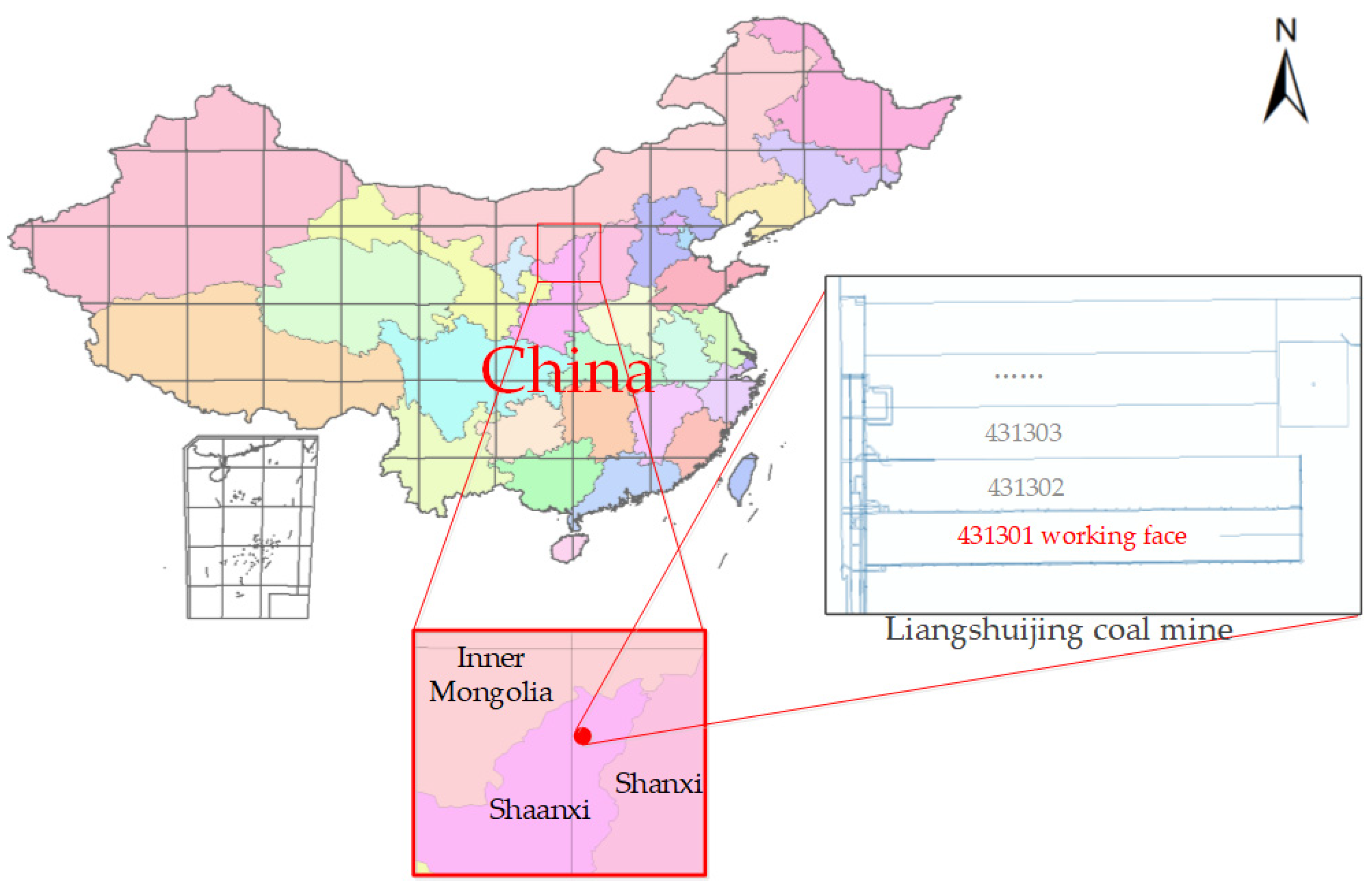
2.1. Study Area
2.1.1. Physical Geography and Environment
2.1.2. Mining and Geological Conditions
2.2. Reference Data
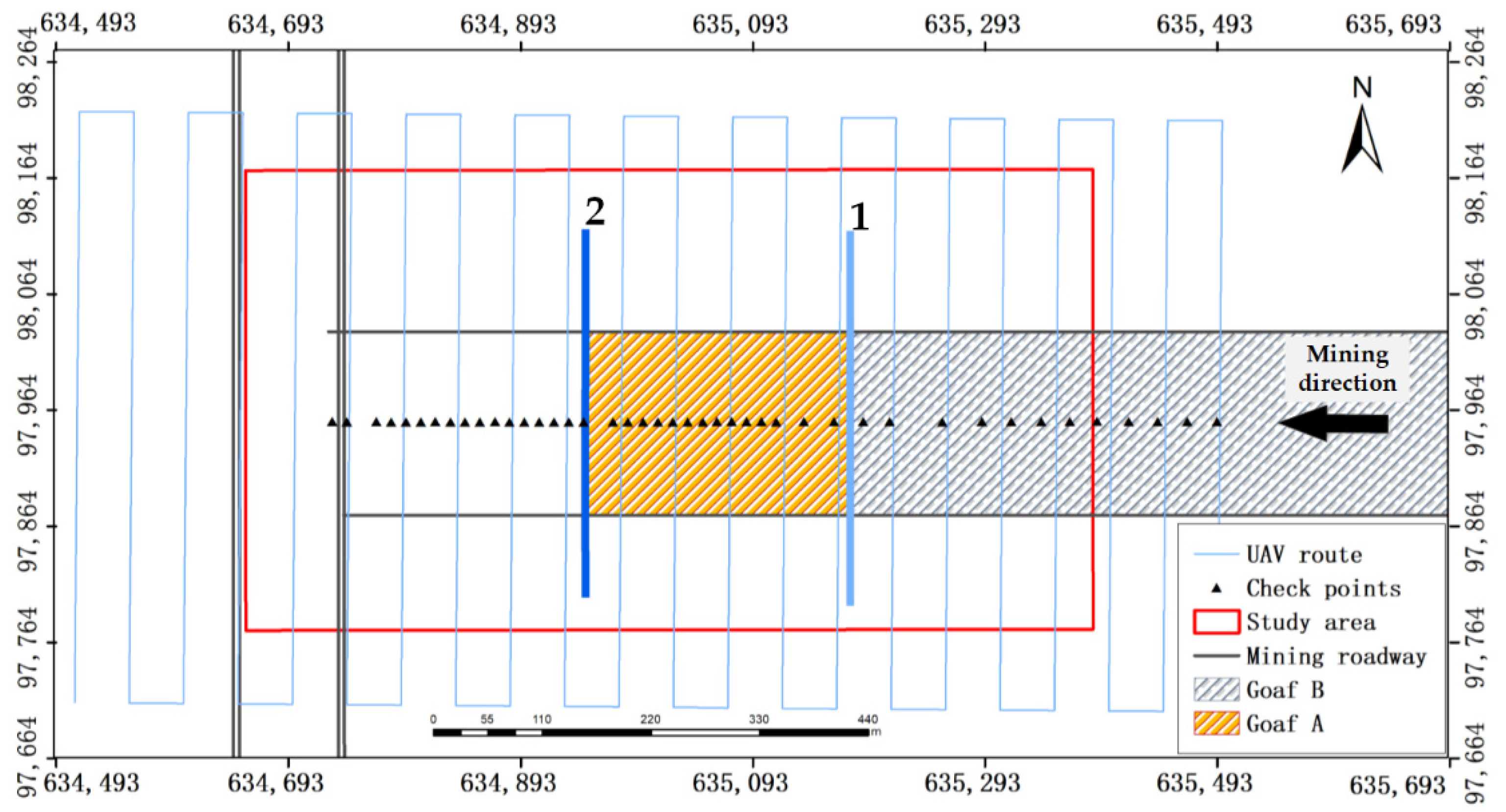
2.2.1. LiDAR Data
2.2.2. Ground Checkpoints
2.3. Data Processing
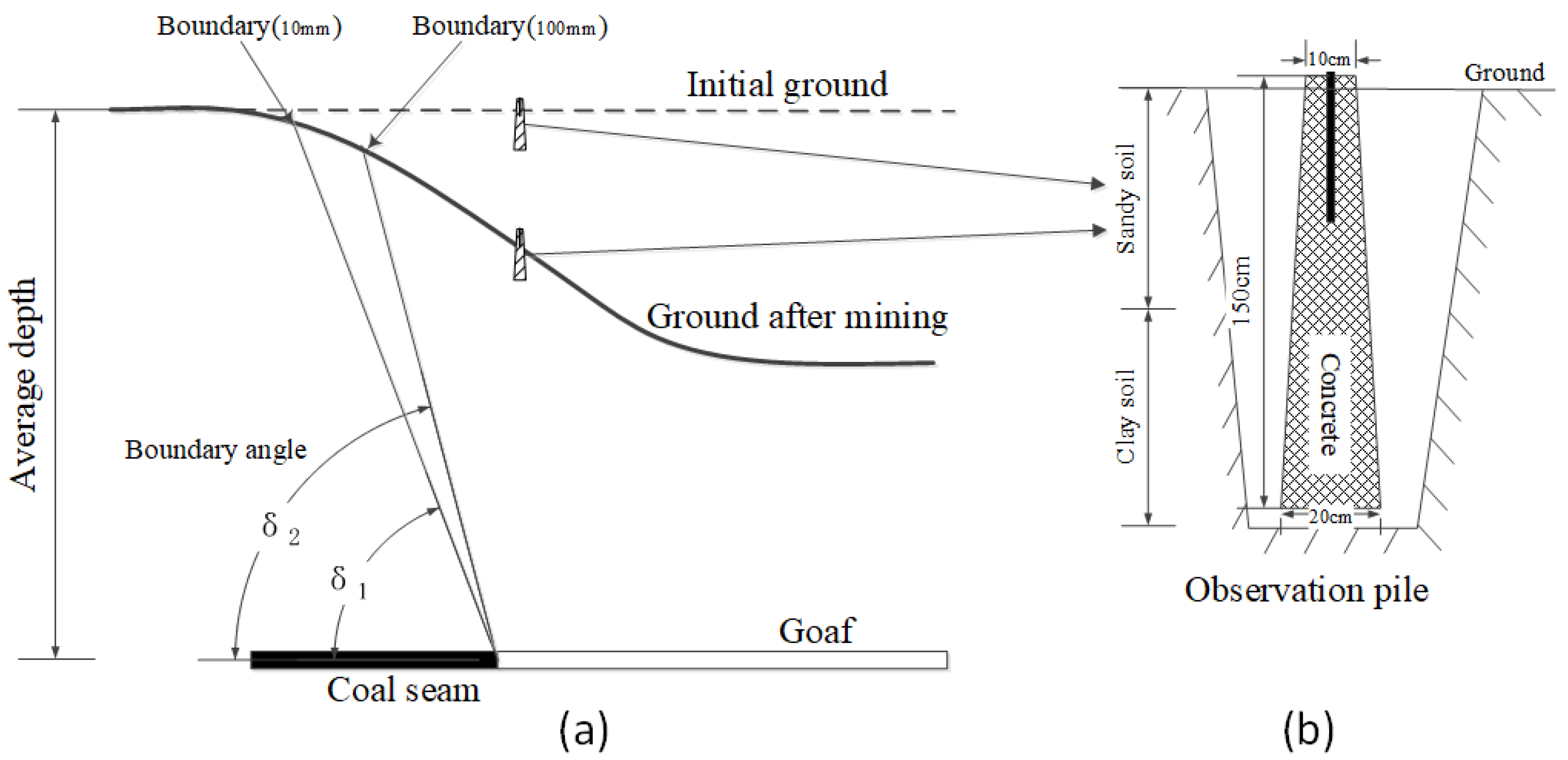
2.3.1. Subsidence Value and Boundary Angle
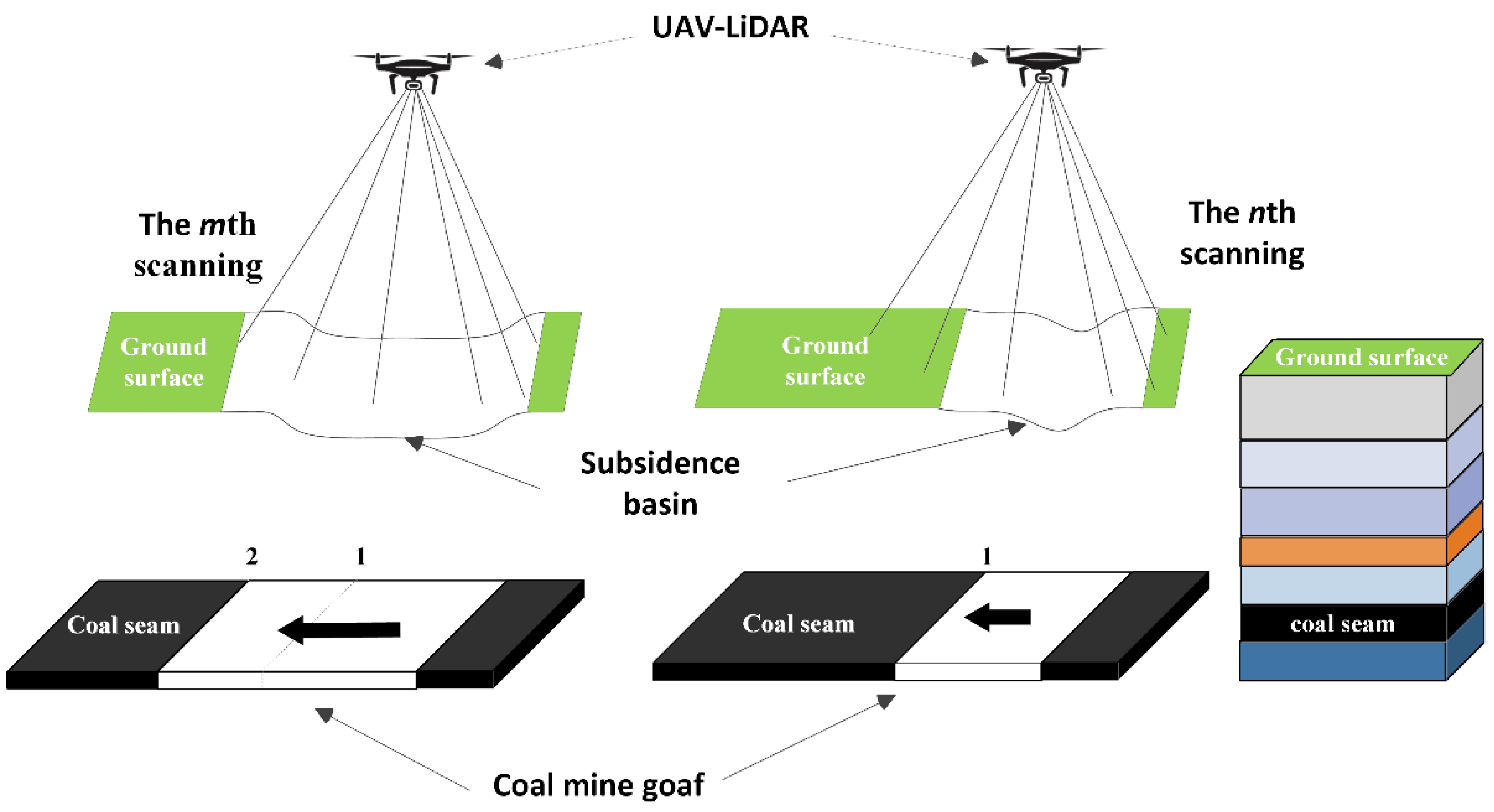
2.3.2. UAV-Based LiDAR Data Processing
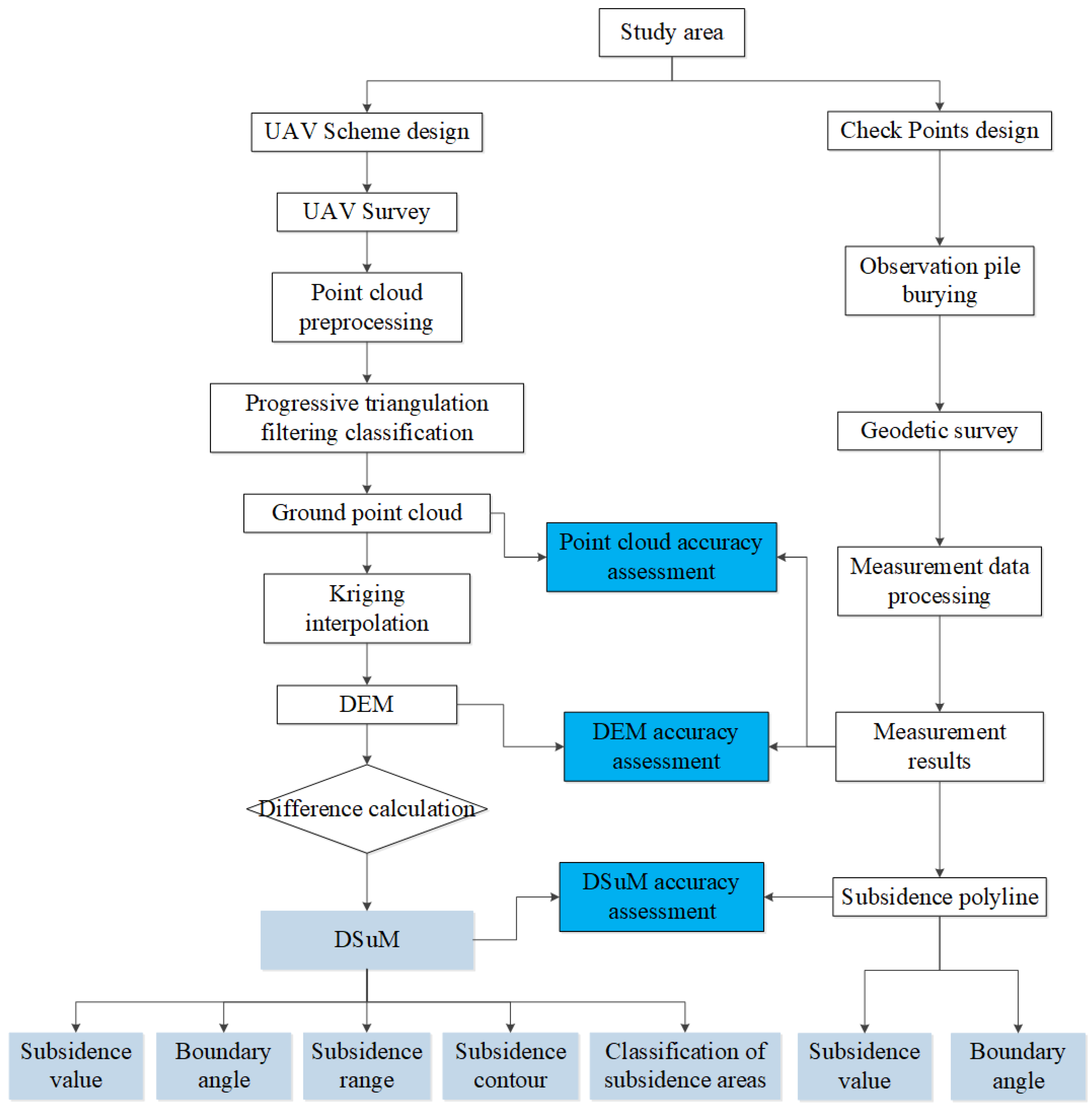
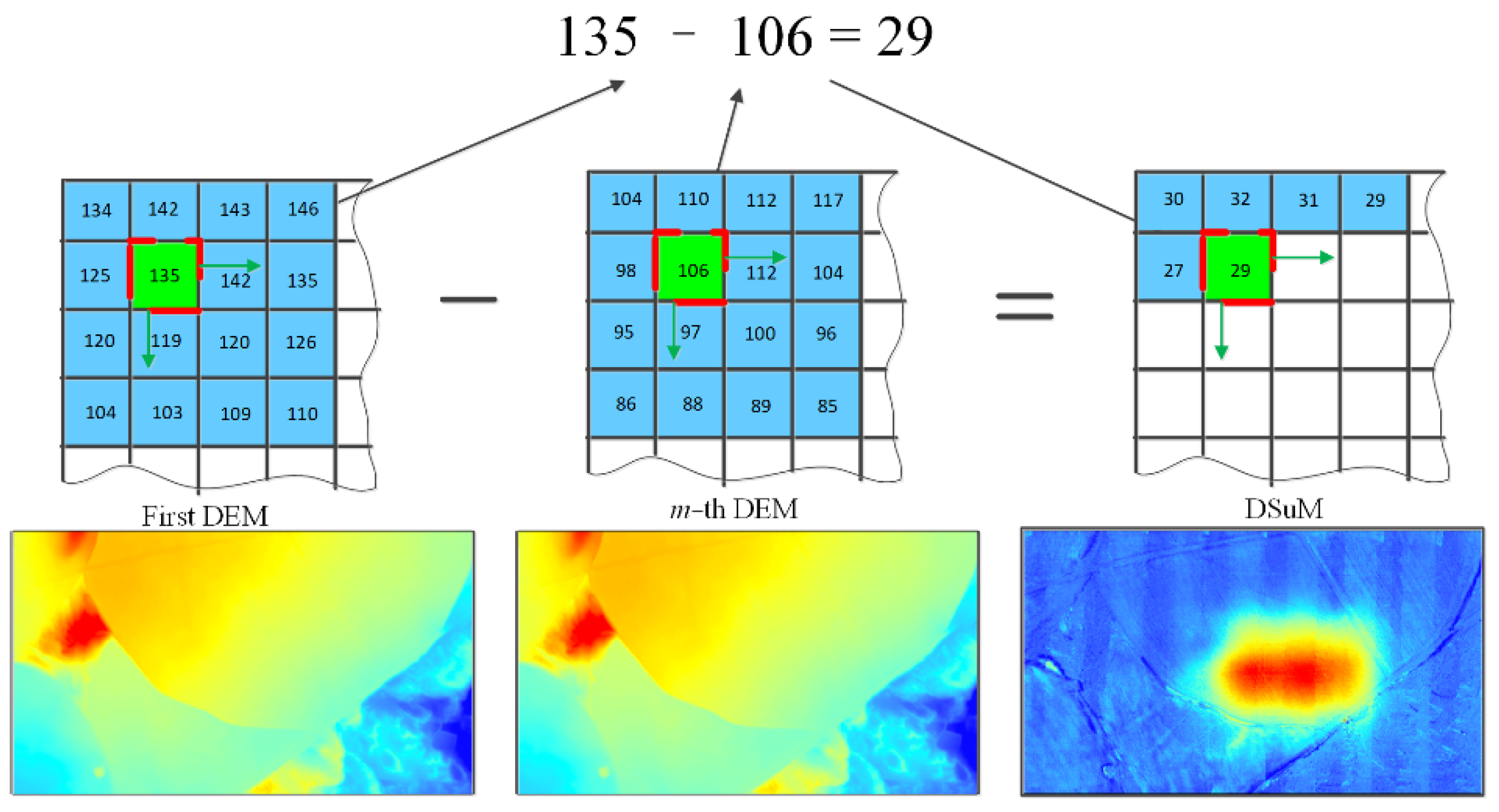
2.4. Pipeline of DSuM
3. Experimental Results
3.1. GCPs Analysis
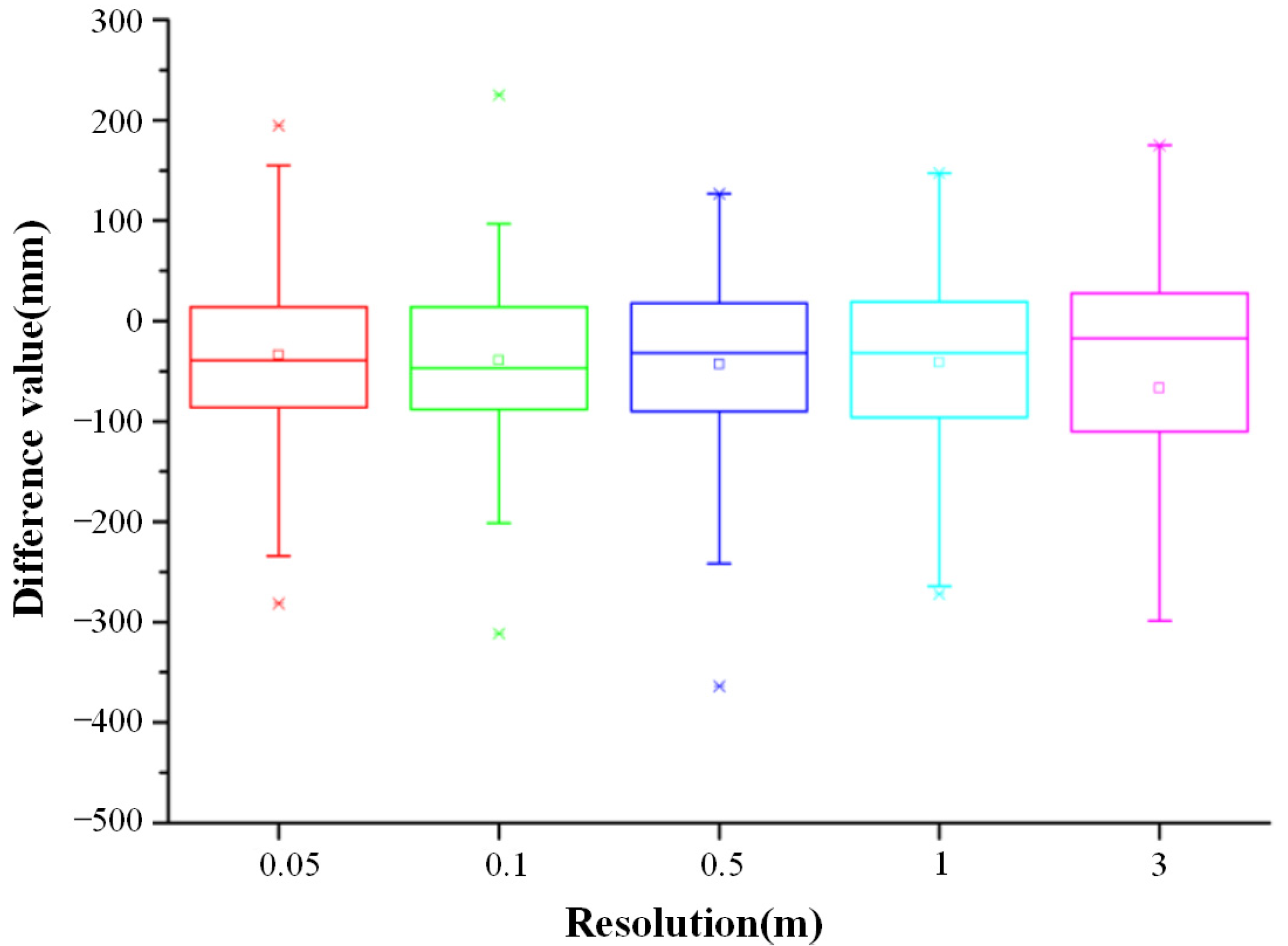
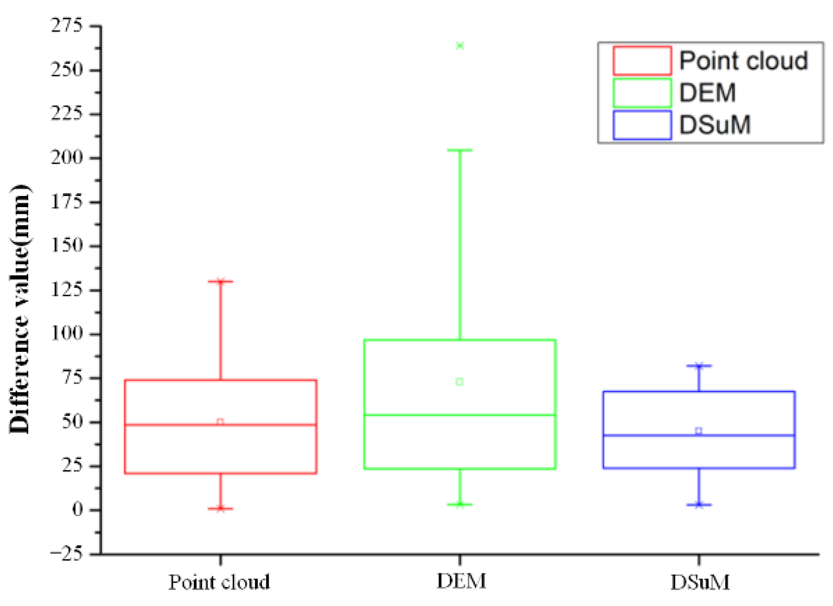
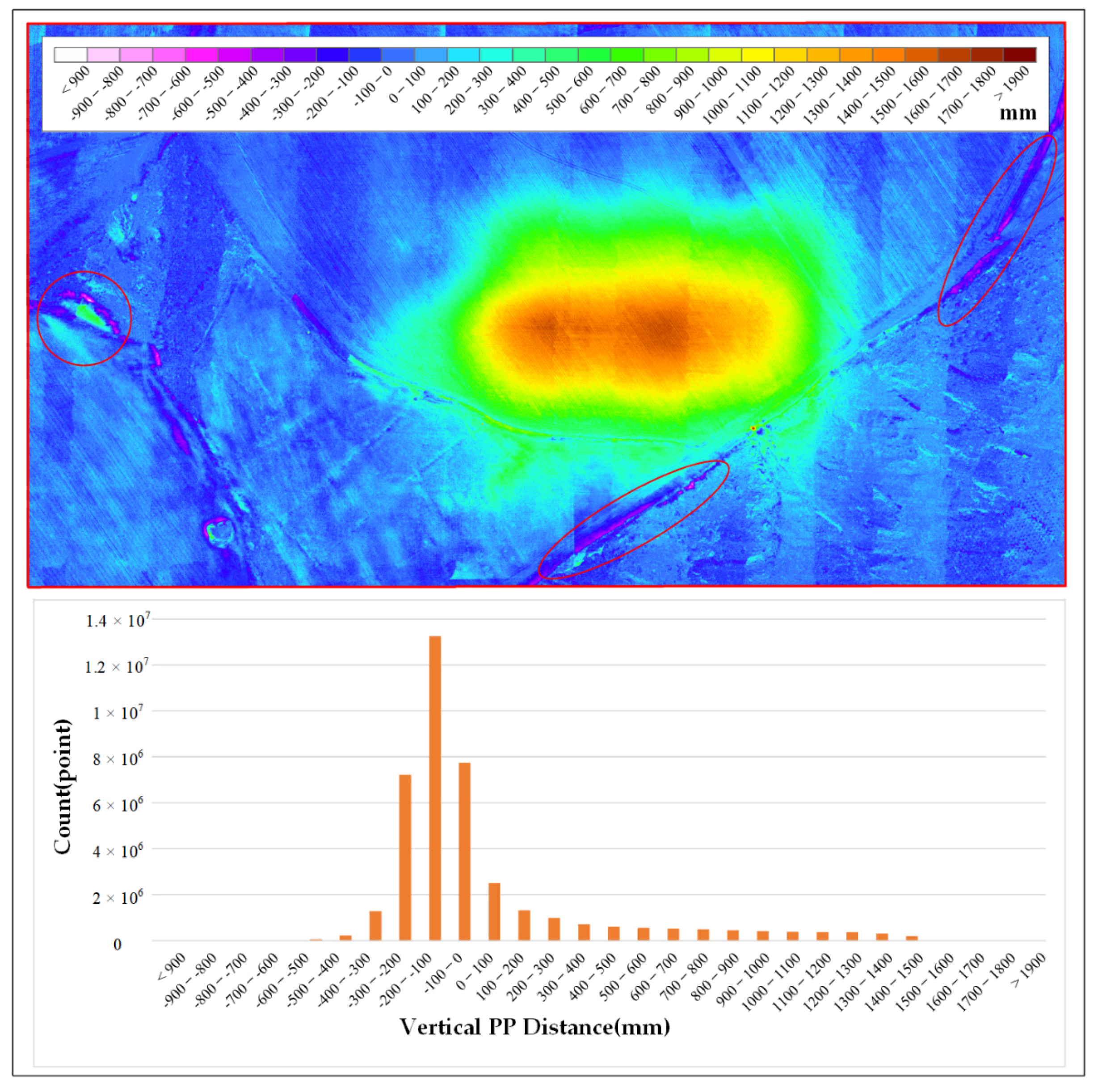
3.2. Accuracy Assessment
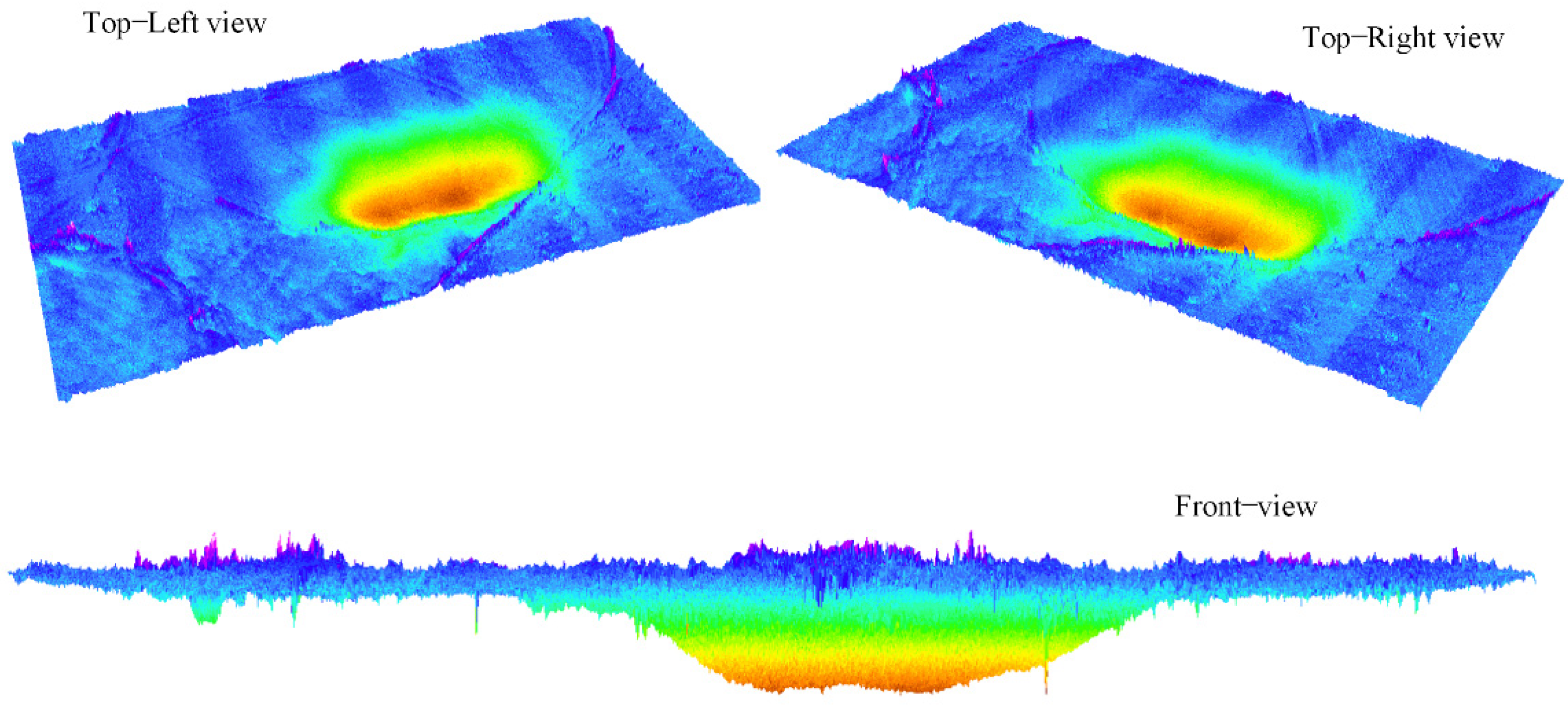
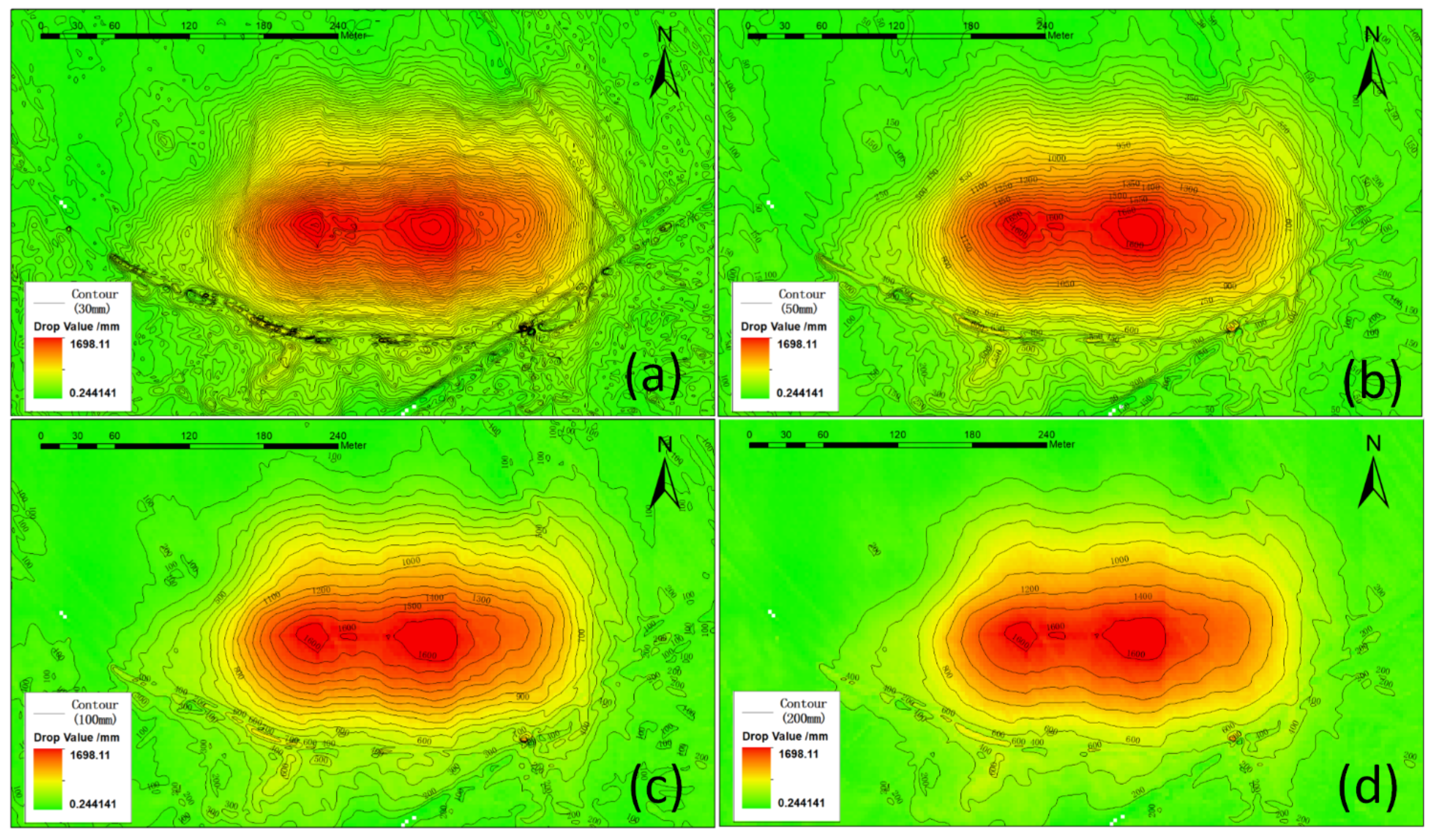
3.3. Analysis of DSuM
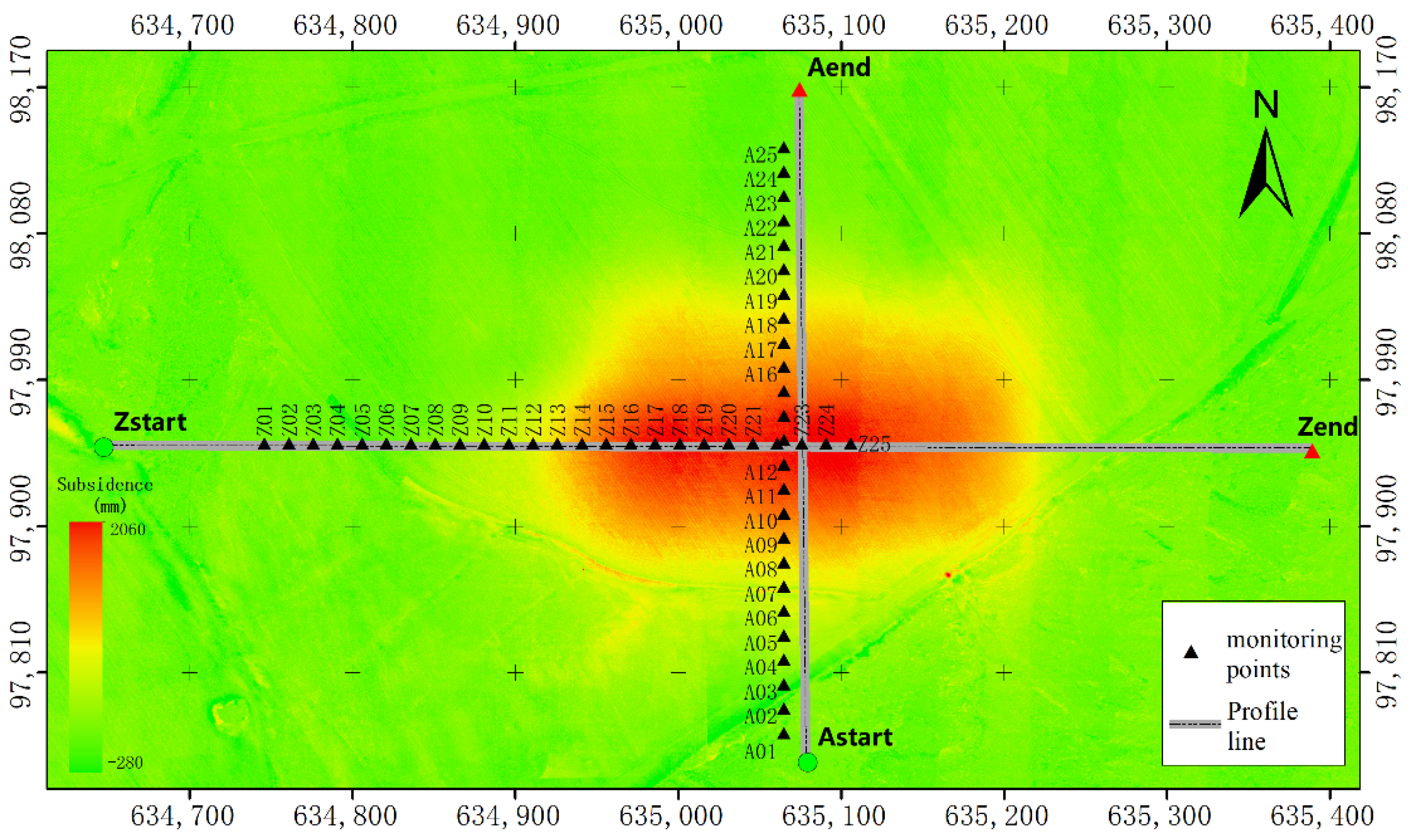
3.3.1. Point Analysis
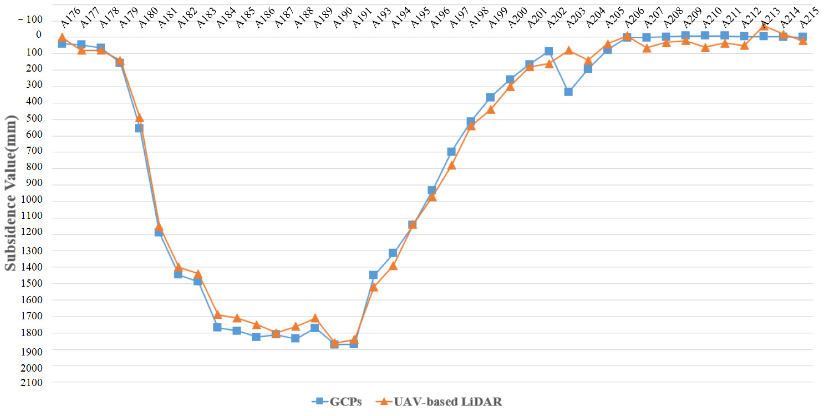
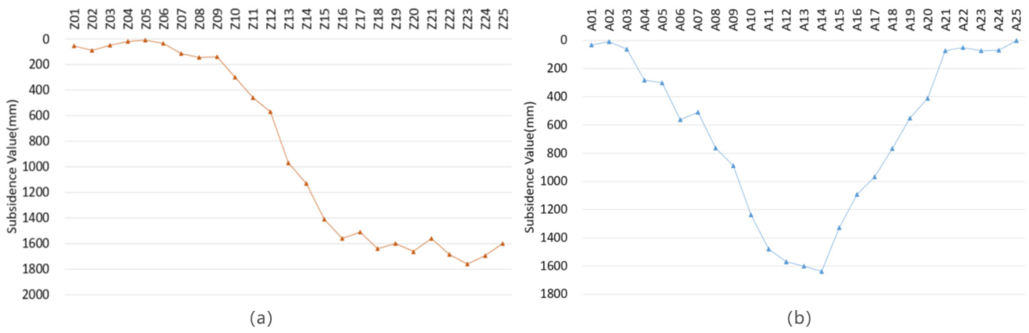
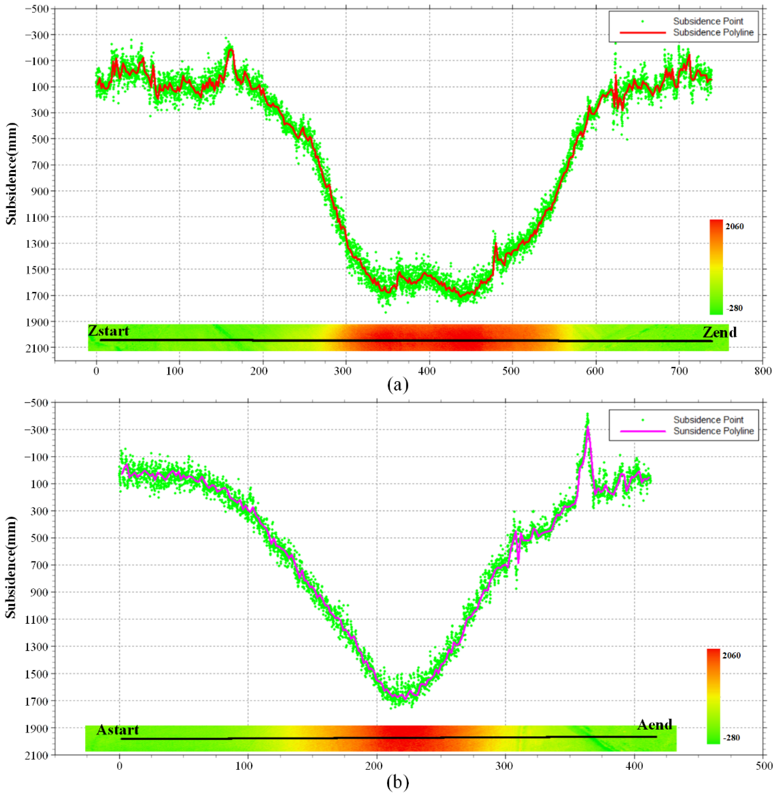
3.3.2. Line Analysis
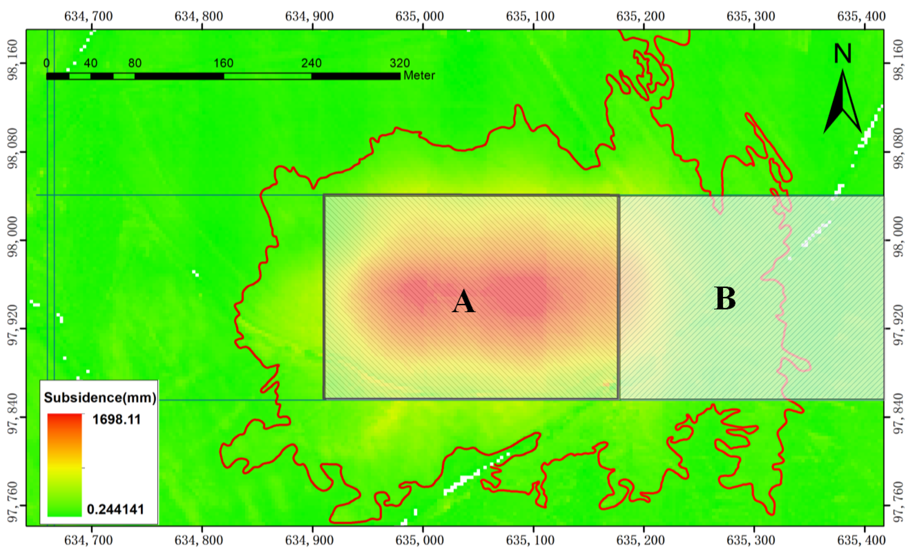
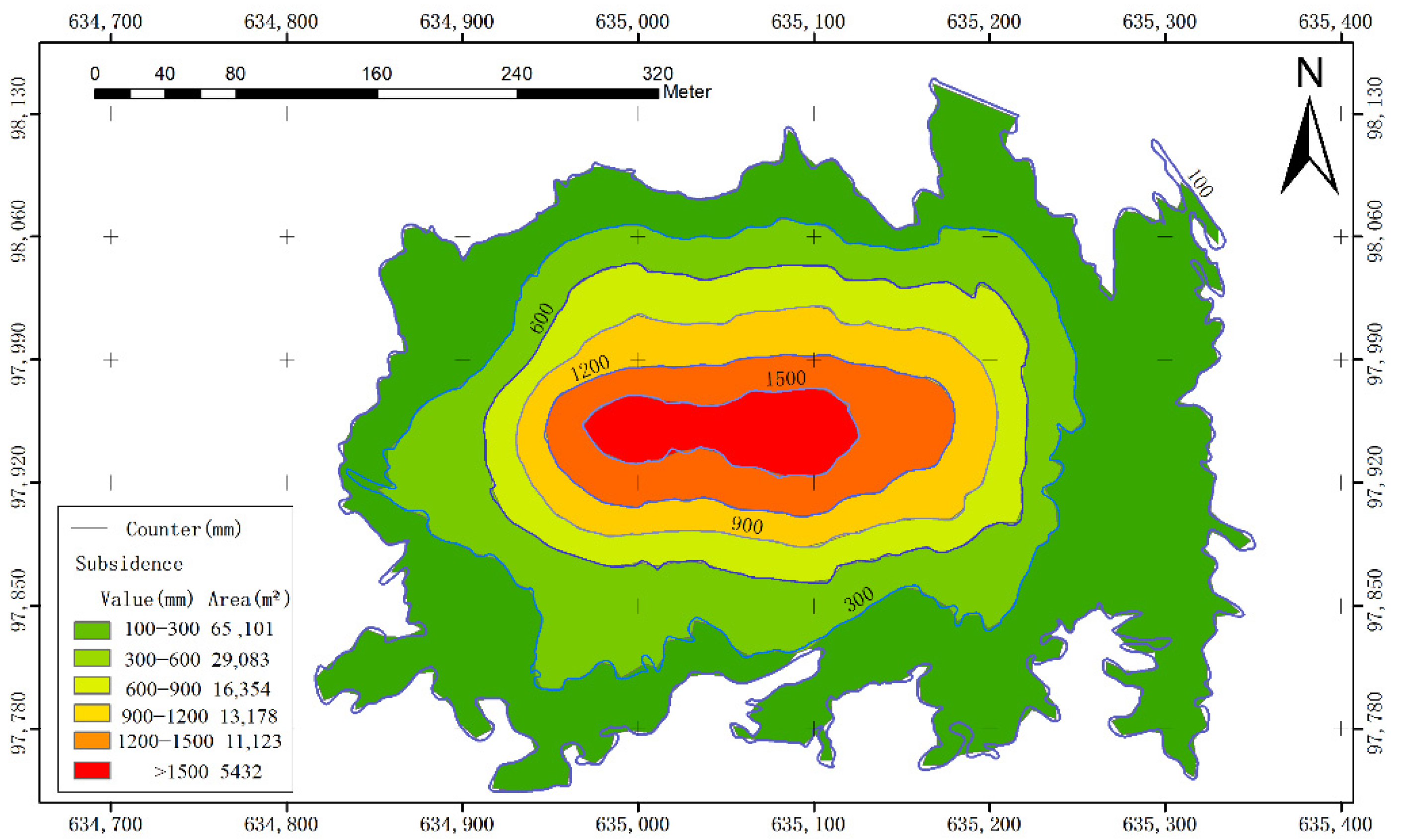
3.3.3. Area Analysis
4. Discussion
5. Conclusions and Future Works
Author Contributions
Funding
Data Availability Statement
Acknowledgments
Conflicts of Interest
References
- Bell, F.G.; Stacey, T.R.; Genske, D.D. Mining subsidence and its effect on the environment: Some differing examples. Environ. Geol. 2000, 40, 135–152. [Google Scholar] [CrossRef]
- Lechner, A.M.; Baumgartl, T.; Matthew, P.; Glenn, V. The impact of underground longwall mining on prime agricultural land: A review and research agenda. Land Degrad. Dev. 2016, 27, 1650–1663. [Google Scholar] [CrossRef]
- Xiao, W.; Fu, Y.; Wang, T.; Lv, X. Effects of land use transitions due to underground coal mining on ecosystem services in high groundwater table areas: A case study in the Yanzhou coalfield. Land Use Policy 2018, 71, 213–221. [Google Scholar] [CrossRef]
- Guo, W.; Barbato, J.; Dai, H.; Peng, S.S.; Agioutantis, Z.; Adhikary, D.; Qu, Q.; Wilkins, A.H.; Poulsen, B.A.; Guo, H.; et al. Surface subsidence damage, mitigation and control. In Surface Subsidence Engineering: Theory and Practice; Peng, S., Ed.; CSIRO Publishing: Clayton, Australia, 2020; pp. 105–131. [Google Scholar]
- Stoch, T. Horizontal Displacement in Mining Area Protection; AGH University of Science and Technology Press: Kraków, Poland, 2019; ISBN 978-83-66364-19-6. [Google Scholar]
- Shi, Y.; Li, J.; Lv, J.; Ma, D. Monitoring and prediction of mining subsidence combined with SBAS-InSAR and support vector regression. Remote Sens. Inf. 2021, 36, 6–12. [Google Scholar]
- Chen, L.; Zhao, X.S. Progress of large gradient deformation monitoring technology in mining area combined with InSAR. Surv. Mapp. Bull. 2018, 7, 18–23. [Google Scholar]
- Pawluszek-Filipiak, K.; Borkowski, A. Integration of DInSAR and SBAS techniques to determine mining-related deformations using Sentinel-1 data: The case study of Rydutowy mine in Poland. Remote Sens. 2020, 12, 242. [Google Scholar] [CrossRef] [Green Version]
- Przyłucka, M.; Herrera, G.; Graniczny, M.; Colombo, D.; Béjar-Pizarro, M. Combination of conventional and advanced DInSAR to monitor very fast mining subsidence with TerraSAR-X data: Bytom city (Poland). Remote Sens. 2015, 7, 5300–5328. [Google Scholar] [CrossRef] [Green Version]
- Rossi, G.; Tanteri, L.; Tofani, V.; Vannocci, P.; Casagli, N. Multitemporal UAV surveys for landslide mapping and characterization. Landslides 2018, 15, 1045–1052. [Google Scholar] [CrossRef] [Green Version]
- Lindner, G.; Schraml, K.; Mansberger, R.; Hübl, J. UAV monitoring and documentation of a large landslide. Appl. Geomat. 2015, 8, 1–11. [Google Scholar] [CrossRef]
- Ge, L.; Li, X.; Ng, H.M. UAV for mining applications: A case study at an open-cut mine and a longwall mine in New South Wales, Australia. In Proceedings of the 2016 IEEE International Geoscience and Remote Sensing Symposium (IGARSS), Beijing, China, 10–15 July 2016. [Google Scholar]
- Tong, X.; Liu, X.; Chen, P.; Liu, S.; Luan, K.; Li, L.; Liu, S.; Liu, X.; Xie, H.; Jin, Y.; et al. Integration of UAV-based photogrammetry and terrestrial laser scanning for the three-dimensional mapping and monitoring of open-pit mine areas. Remote Sens. 2015, 7, 6635–6662. [Google Scholar] [CrossRef] [Green Version]
- Lian, X.; Liu, X.; Ge, L.; Hu, H.; Wu, Y. Time-series unmanned aerial vehicle photogrammetry monitoring method without ground control points to measure mining subsidence. J. Appl. Remote Sens. 2021, 15, 024505. [Google Scholar] [CrossRef]
- Ignjatovi Stupar, D.; Roer, J.; Vuli, M. Investigation of unmanned aerial vehicles-based photogrammetry for large mine subsidence monitoring. Minerals 2020, 10, 196. [Google Scholar] [CrossRef] [Green Version]
- Chen, P. Research on Mining Subsidence Monitoring Method of UAV Tilt Photogrammetry. Master’s Thesis, Taiyuan University of Technology, Taiyuan, China, 2018. [Google Scholar]
- Wikaa, P.; Gruszczyński, W.; Stoch, T.; Puniach, E.; Wójcik, A. UAV Applications for determination of land deformations caused by underground mining. Remote Sens. 2020, 12, 1733. [Google Scholar] [CrossRef]
- Zhou, D.; Qi, L.; Zhang, D.; Zhou, B.; Guo, L. Unmanned aerial vehicle (UAV) photogrammetry technology for dynamic mining subsidence monitoring and parameter inversion: A case study in China. IEEE Access 2020, 8, 16372–16386. [Google Scholar] [CrossRef]
- Rauhala, A.; Tuomela, A.; Davids, C.; Rossi, P.M. UAV remote sensing surveillance of a mine tailings impoundment in sub-arctic conditions. Remote Sens. 2017, 9, 1318. [Google Scholar] [CrossRef] [Green Version]
- Martínez-Carricondo, P.; Mesas-Carrascosa, F.J.; García-Ferrer, A.; Agüera-Vega, F.; Pérez-Porras, F.J. Assessment of UAV-photogrammetric mapping accuracy based on variation of ground control points. Int. J. Appl. Earth Obs. Geoinf. 2018, 72, 1–10. [Google Scholar] [CrossRef]
- Johan, K.; Christophe, D.; Pascal, A.; Pierre, P.; Marion, J.; Eric, V. Application of a terrestrial laser scanner (TLS) to the study of the Séchilienne landslide (Isère, France). Remote Sens. 2010, 2, 2785–2802. [Google Scholar] [CrossRef] [Green Version]
- Guo, C.; Li, J.; Feng, H.; Zhao, J. Application of 3D laser scanning technology in dam subsidence monitoring in mining area. Mine Surv. 2014, 6, 70–72. [Google Scholar] [CrossRef]
- Bai, W. Monitoring mining subsidence by three-dimensional laser scanning technology. Metal Mines 2017, 1, 132–135. [Google Scholar] [CrossRef]
- Gu, Y.; Zhou, D.; Zhang, D.; Wu, K.; Zhou, B. Study on subsidence monitoring technology using terrestrial 3D laser scanning without a target in a mining area: An example of Wangjiata coal mine, China. Bull. Eng. Geol. Environ. 2020, 79, 3575–3583. [Google Scholar] [CrossRef]
- Brede, B.; Lau, A.; Bartholomeus, H.M.; Kooistra, L. Comparing RIEGL RiCOPTER UAV LiDAR derived canopy height and DBH with terrestrial LiDAR. Sensors 2017, 17, 2371. [Google Scholar] [CrossRef] [PubMed]
- Yu, H.; Lu, X.; Gang, C.; Ge, X. Detection and volume estimation of mining subsidence based on multi-temporal LiDAR data. In Proceedings of the 19th International Conference on Geoinformatics (IEEE 2011), Shanghai, China, 24–26 June 2011; pp. 1–6. [Google Scholar] [CrossRef]
- Yu, H.; Lu, X.; Ge, X.; Cheng, G. Digital terrain model extraction from airborne LiDAR data in complex mining area. In Proceedings of the 18th International Conference on Geoinformatics (IEEE 2010), Beijing, China, 18–20 June 2010. [Google Scholar]
- Ao, J.; Wu, K.; Wang, Y.; Li, L. Subsidence monitoring using lidar and morton code indexing. J. Surv. Eng. 2016, 142, 06015002. [Google Scholar] [CrossRef]
- Elsner, P.; Dornbusch, U.; Thomas, I.; Dan, A.; Bovington, J.; Horn, D. Coincident beach surveys using UAS, vehicle mounted and airborne laser scanner: Point cloud inter-comparison and effects of surface type heterogeneity on elevation accuracies. Remote Sens. Environ. 2018, 208, 15–26. [Google Scholar] [CrossRef]
- Siranec, M.; Hger, M.; Otcenasova, A. Advanced power line diagnostics using point cloud data—Possible applications and limits. Remote Sens. 2021, 13, 1880. [Google Scholar] [CrossRef]
- Bakuła, K.; Pilarska, M.; Salach, A.; Kurczyński, Z. Detection of levee damage based on UAS data—Optical imagery and LiDAR point clouds. Int. J. Geo-Inf. 2020, 9, 248. [Google Scholar] [CrossRef] [Green Version]
- Chen, Q.; Hang, M.; Li, J.; Wang, X. Study on extraction method of vegetation restoration height in mining area based on lidar. Coal Sci. Technol. 2020, 48, 113–119. [Google Scholar]
- Streutker, D.R.; Glenn, N.F. LiDAR measurement of sagebrush steppe vegetation heights. Remote Sens. Environ. 2006, 102, 135–145. [Google Scholar] [CrossRef]
- Song, S. Quantitative Evaluation of Ecological Environment Damage Caused by Coal Mining in Yushenfu Mining Area. Master’s Thesis, Xi’an University of Science and Technology, Xi’an, China, 2009. [Google Scholar]
- Hsieh, Y.C.; Chan, Y.C.; Hu, J.C. Digital elevation model differencing and error estimation from multiple sources: A case study from the Meiyuan Shan landslide in Taiwan. Remote Sens. 2016, 8, 199. [Google Scholar] [CrossRef] [Green Version]
- Chen, Q.; Wang, H.; Zhang, H.; Sun, M.; Liu, X. A point cloud filtering approach to generating DTMs for steep mountainous areas and adjacent residential areas. Remote Sens. 2016, 8, 71. [Google Scholar] [CrossRef] [Green Version]
- Salach, A.; Bakua, K.; Pilarska, M.; Ostrowski, W.; Górski, K.; Kurczyński, Z. Accuracy assessment of point clouds from LiDAR and dense image matching acquired using the UAV platform for DTM creation. Int. J. Geo-Inf. 2018, 7, 342. [Google Scholar] [CrossRef] [Green Version]
- Yang, B.; Huang, R.; Dong, Z.; Li, J. Two-step adaptive extraction method for ground points and breaklines from lidar point clouds. ISPRS J. Photogramm. Remote Sens. 2016, 119, 373–389. [Google Scholar] [CrossRef]
- Axelsson, P. DEM generation from laser scanner data using adaptive TIN models. Int. Arch. Photogramm. Remote Sens. 2000, 33, 110–117. [Google Scholar]
- Jiao, X.H. Research on Airborne LiDAR Point Cloud Filtering Algorithm and DEM Interpolation Method. Master’s Thesis, Taiyuan University of Technology, Taiyuan, China, 2018. [Google Scholar]
- Kang, S.; Ji, L.; Jiao, Q.; Zhang, J. Comparative study on interpolation methods based on ground lidar point cloud data. Geod. Geodyn. 2020, 4, 400–404. [Google Scholar] [CrossRef]
- Dougherty, E.R. An Introduction to Morphological Image Processing; SPIE Optical Engineering Press: Bellingham, WA, USA, 1992. [Google Scholar]
- Maciuk, K.; Lewińska, P. High-rate monitoring of satellite clocks using two methods of averaging time. Remote Sens. 2019, 11, 2754. [Google Scholar] [CrossRef] [Green Version]


| Date | Study Area (m2) | Number of Points | Point Cloud Density (per/m2) | Number of Ground Points | Ground Point Cloud Density (per/m2) |
|---|---|---|---|---|---|
| 7 November 2020 | 399,431 | 35,590,816 | 89 | 33,227,279 | 83 |
| 19 May 2021 | 399,431 | 26,361,111 | 66 | 21,776,124 | 55 |
| Date | Max (mm) | Min (mm) | Ave (mm) | Med (mm) | RMSE (mm) |
|---|---|---|---|---|---|
| 7 November 2020 | 130.0 | 1.0 | 50.0 | 48.5 | 60.6 |
| 19 May 2021 | 113.0 | 4.0 | 51.5 | 47.5 | 59.9 |
| Grid Size (m) | ME (mm) | MAE (mm) | RMSE (mm) |
|---|---|---|---|
| 0.05 | −34 | 74 | 97 |
| 0.1 | −39 | 79 | 106 |
| 0.5 | −43 | 77 | 109 |
| 1 | −41 | 76 | 102 |
| 3 | −67 | 106 | 167 |
| 5 | −89 | 157 | 248 |
| 10 | −4 | 165 | 238 |
| 20 | 323 | 537 | 926 |
| Subsidence Value (mm) | Number of Pixels | Resolution (m) | Area (m2) | Area Ratio (%) | Subsidence Area Ratio (%) |
|---|---|---|---|---|---|
| <100 | 22,062,688 | 0.1 | 220,627 | 55.1 | - |
| 100–300 | 10,258,459 | 0.1 | 102,585 | 25.6 | 57.0 |
| 300–600 | 3,033,611 | 0.1 | 30,336 | 7.6 | 16.8 |
| 600–900 | 1,710,181 | 0.1 | 17,102 | 4.3 | 9.5 |
| 900–1200 | 1,341,367 | 0.1 | 13,414 | 3.3 | 7.4 |
| 1200–1500 | 1,116,807 | 0.1 | 11,168 | 2.8 | 6.2 |
| 1500–1700 | 516,812 | 0.1 | 5168 | 1.3 | 2.9 |
| >1700 | 30,187 | 0.1 | 302 | 0.1 | 0.2 |
Publisher’s Note: MDPI stays neutral with regard to jurisdictional claims in published maps and institutional affiliations. |
© 2022 by the authors. Licensee MDPI, Basel, Switzerland. This article is an open access article distributed under the terms and conditions of the Creative Commons Attribution (CC BY) license (https://creativecommons.org/licenses/by/4.0/).
Share and Cite
Zheng, J.; Yao, W.; Lin, X.; Ma, B.; Bai, L. An Accurate Digital Subsidence Model for Deformation Detection of Coal Mining Areas Using a UAV-Based LiDAR. Remote Sens. 2022, 14, 421. https://doi.org/10.3390/rs14020421
Zheng J, Yao W, Lin X, Ma B, Bai L. An Accurate Digital Subsidence Model for Deformation Detection of Coal Mining Areas Using a UAV-Based LiDAR. Remote Sensing. 2022; 14(2):421. https://doi.org/10.3390/rs14020421
Chicago/Turabian StyleZheng, Junliang, Wanqiang Yao, Xiaohu Lin, Bolin Ma, and Lingxiao Bai. 2022. "An Accurate Digital Subsidence Model for Deformation Detection of Coal Mining Areas Using a UAV-Based LiDAR" Remote Sensing 14, no. 2: 421. https://doi.org/10.3390/rs14020421