A Novel Tropical Cyclone Size Estimation Model Based on a Convolutional Neural Network Using Geostationary Satellite Imagery

Abstract

A novel tropical cyclone (TC) size estimation model (TC-SEM) in the western North Pacific was developed based on a convolutional neural network (CNN) using geostationary satellite infrared (IR) images. The proposed TC-SEM was tested using three CNN schemes: a single-task regression model that separately estimated the radius of maximum wind (RMW) and the radius of 34 kt wind (R34) of the TC, a multi-task regression model that estimated the RMW and R34 simultaneously, and a multi-task regression model using best-track TC intensity information. For model training, validation, and testing, 29,730, 2505, and 11,624 geostationary satellite images of the region around the center of the TC, respectively, were used, each containing four IR bands: short-wavelength IR (3.7 µm), water vapor (6.7 µm), IR1 (10.8 µm), and IR2 (12.0 µm). The results showed that the multi-task model performed better than the single-task model due to knowledge sharing and its ability to solve multiple interrelated tasks simultaneously. The inclusion of TC intensity information in the multi-task model further improved the performance of the RMW and R34 estimations, with correlations (mean absolute errors) of 0.95 (2.05 nmi) and 0.93 (9.77 nmi), respectively, which represent significant improvements over the performance of existing linear regression statistical methods. The results suggested that this CNN model using geostationary satellite images may be a powerful tool for estimating TC sizes in operational TC forecasts.

1. Introduction

Tropical cyclones (TCs), which are low-pressure systems that form over warm tropical waters and are accompanied by strong winds and torrential rain, represent one of the gravest threats to the lives and properties of coastal communities. When a TC approaches a landmass, it is crucial to predict its impact area for disaster preparedness. TC size information, which indicates the TC impact area, is routinely provided by global TC warning centers during TC seasons [1]. In general, TC size is measured using various wind-based parameters, such as the radius of maximum wind (RMW), radius of gale-force wind (i.e., 34 kt; R34; 1 kt = 0.514 m s⁻¹), radius of damaging-force wind (i.e., 50 kts; R50), radius of hurricane-force wind (i.e., 64 kt; R64), and radius of the outermost closed isobars (ROCI) [2,3,4,5,6,7]. Among these radii, the RMW is a basic parameter used to estimate TC wind structure, and R34 is the most widely used parameter because it determines the potential impact area of a TC [8,9,10,11].

TCs spend most of their lifetimes in the open ocean, where in situ observations are very rare. Therefore, TC size estimation relies heavily on satellite observations and information obtained using scatterometers [12], microwave sounders [13,14], and infrared (IR) images [15,16,17,18,19,20,21,22,23]. Of these, IR-based methods are the most widely used in real-time operations due to the continuous stream of satellite images [16,18]. Currently, multiple satellite-based techniques, which combine information from scatterometry, cloud/feature-tracked winds, microwave sounders, and IR methods [20], are employed in TC warning centers.

Demuth et al. [14] objectively estimated azimuthally averaged R34, R50, and R64 for TCs using Advanced Microwave Sounding Unit (AMSU) data from the National Oceanic and Atmospheric Administration (NOAA)-15, 16, and 17 satellites for the Atlantic and eastern Pacific for the period 1999–2004. These data are too coarse to adequately resolve TC structures because the spatial resolution is 48 km. Therefore, for almost real-time and objective estimations of TC sizes, a linear-regression-based statistical model (best-subsets multiple linear regression combined with a cross-validation method) was developed using 24 estimative parameters, including parameters derived from the AMSU, and introduced into the operation of the National Hurricane Center/Tropical Prediction Center in 2005. However, due to the coarse spatial resolution of the AMSU, this method cannot accurately estimate the winds in the inner cores of TCs.

To overcome this problem, various techniques have been developed based on satellite IR data. Kossin et al. [23] found that in cases of clear-eye TCs in IR images of geostationary satellites, the RMW can be indirectly estimated through a regression relationship with the IR-measured eye size. In general cases without IR scene-type constraints, they indirectly estimated the RMW and azimuthally averaged R34, R50, and R64 through a regression relationship using storm intensity, storm location, storm age, and principal components retrieved from IR images. The estimated RMW and wind radius were used to compensate for the inner-core TC areas, for which there were no data due to aircraft reconnaissance unavailability.

On the other hand, Knaff et al. [20] indirectly calculated the wind radii of the quadrant as a regression method using the threshold values and shape parameters of R34, R50, and R64 for each azimuth, which were based on the 850-hPa mean tangential wind at a radius of 500 km and the radius of 5-kt winds estimated from IR images and storm information. Kossin et al. [23] and Knaff et al. [20] also estimated TC wind radii by employing a relatively simple method using routinely available information based on IR images. However, these methods perform poorly when TCs are highly asymmetrical and/or undergo extratropical transition characterized by the absence of a deep convective signal, fast movement, and/or occurrence at high latitudes. These direct/indirect TC wind radius estimation methods are limited to the Atlantic and eastern Pacific basins for which there are aircraft reconnaissance data.

In the western North Pacific, TC wind radii are primarily determined using all available observation instruments and data, including satellite IR images, radar, surface synoptic observations, ships, buoys, the Advanced Scatterometer [24], Multiplatform Tropical Cyclone Surface Wind Analysis [25], and microwave radiometers [26]. When these data are not available, the TC wind radii are indirectly estimated from the regression between wind radii and maximum wind speed using IR satellite data [17,18] and the regression between central pressure and wind radius [27]. However, each of these linear-regression-based methods is known to have its own weaknesses [18,27] that lead to errors in operational and best-track wind radius estimates, which may be as large as 25–40% of the radii [8,20,21,22,23,24,25,26,27].

Recently, convolutional neural networks (CNNs), an artificial intelligence deep learning technique [28], have been used in TC studies in conjunction with satellite-based TC image analysis [29,30,31,32,33,34,35,36]. However, despite the importance of TC size, most previous studies utilized CNNs only to estimate the TC intensity and tracks [29,30,31,32,33,34,35,36]. This study aimed to address this research gap by proposing an objective TC size estimation technique using a CNN model and geostationary satellite-based multispectral images from the western North Pacific (WNP). The study’s methods were benchmarked against a previously constructed CNN model for TC intensity estimation [32].

The rest of this paper is organized as follows. Section 2 describes the dataset, CNN model, specific parameters, and model optimization methods used in this study. Section 3 presents the training, validation, and testing results; provides an interpretation of the model; and discusses the results of sensitivity experiments. Section 4 summarizes the findings and presents the conclusions.

2. Data and Model Design

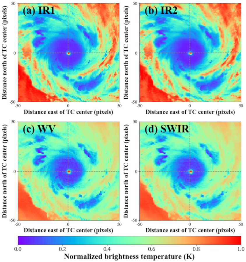
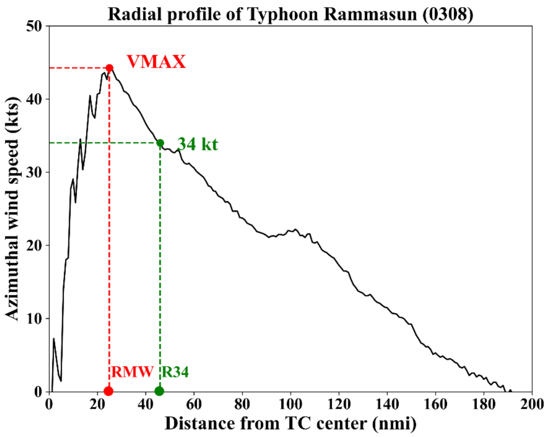
2.1. Data

A TC size estimation model (TC-SEM) was developed using geostationary satellite IR images from the Communication, Ocean, and Meteorological Satellite (COMS) Meteorological Imager (MI) of all TCs that occurred in the WNP during 2011–2016. The analysis period was selected based on the simultaneous availability of COMS MI data and TC intensity and size (for example, RMW and R34) information. Launched in 2010, the COMS is the first Korean multifunction geostationary satellite and is stationed at 128.2° E and 36,000 km above Earth’s equator [37]. The satellite has three payloads: one for meteorology, one for ocean observation, and one for communications. Its MI sensor for meteorology observes one side of the Earth every 15 min, with a horizontal spatial resolution of 1–4 km. The sensor consists of five spectral channels (one visible light and four IR). The visible light sensor has a spatial resolution of 1 km and a central wavelength of 0.67 µm. The IR channel has a spatial resolution of 4 km and contains four bands: short-wavelength IR (SWIR; 3.7 µm), water vapor (WV; 6.7 µm), IR1 (10.8 µm), and IR2 (12.0 µm) (Figure 1).

These four IR bands are sufficient to identify cloud features in the upper, upper-middle, middle, and lower atmospheres, respectively, making it possible to identify the vertical structures of TCs to some extent [32,38,39,40,41]. They also capture cloud features of the outer regions of TCs, including shallow rainbands and nonprecipitating anvil clouds [33].

TC information was obtained from the International Best Track Archives for Climate Stewardship (IBTrACS), version 4. Best-track data, representing the best estimates of TC parameters, are provided by many agencies around the world, but each agency records slightly different TC characteristics in a variety of formats. This creates numerous problems when generating global datasets, such as different agencies reporting very different locations and intensities for the same TC. Moreover, the maximum sustained wind speed reported by various agencies is based on different definitions (e.g., 1, 3, and 10 min sustained winds). To address these problems, the NOAA’s National Climatic Data Center (NCDC) developed the IBTrACS, which is a novel, homogeneous, and comprehensive global TC best-track dataset collected by 12 agencies around the globe [42]. The recorded data, updated every 6 h, include TC location (longitude and latitude), intensity (maximum wind speed and minimum sea-level pressure), and size (RMW, R34, R50, R64, and ROCI; for R34, R50, and R64, quadrant data are provided [42,43]).

Figure 2 shows a schematic diagram indicating the RMW and R34 in the TC wind section. In this study, the RMW and mean R34 (average of R34 quadrants) were used for the label data, which were the values to be estimated by the TC-SEM. The label data were used after interpolation at the observation time of the COMS MI data.

When using machine learning techniques, including CNNs, it is important to ensure that the training data are evenly distributed (that is, the sample size should not be too large or too small for a specific bin) and that the features of the data are well reflected. In this study, TC images of 301 × 301 pixels (i.e., 1204 × 1204 km) were extracted from the four IR channels of the COMS MI using the TC center location obtained from the IBTrACS data [32]. The extracted TC images were reconstructed into 101 × 101-pixel images with a horizontal spatial resolution of about 12 km for computational efficiency. To balance the dataset, samples were randomly removed from bins with large sample sizes. The dataset was then augmented through two oversampling processes—temporal interpolation and image rotation—for bins with small sample sizes. Moreover, the label data were normalized from 0 to 1 by dividing the RMW and R34 by their respective maximum values to compare the “loss” and “validation loss” in the CNN model. The dataset used in this study was randomly divided into training, validaion, and test sets in a ratio of 68:6:26 (

Table 1. Sample data used in the study. The data were balanced using the method of Lee et al. [32].

Data Set	Sample Size
Training	29,730
Validation	2505
Testing	11,624
Total	43,859

). The training dataset was used to fit the weights that matched the “ground truth” data in the CNN model. The validation dataset was used to identify the best hyperparameters in the model. Finally, the best-performing CNN scheme identified using the validation dataset was applied to the test data to perform an independent assessment of its performance.

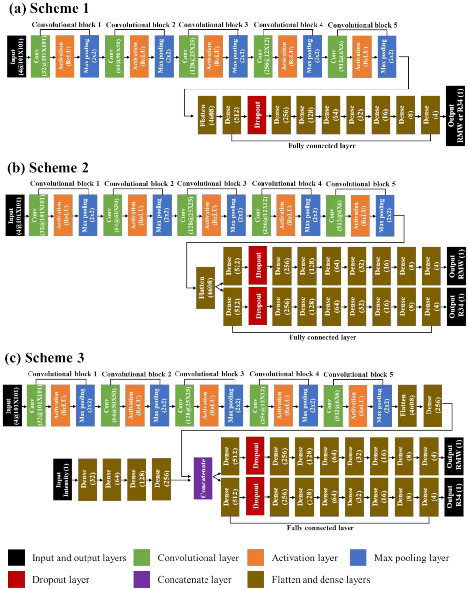
2.2. Convolutional Neural Network (CNN)

A CNN is a hierarchical neural network system that can extract and analyze feature vectors from complex multidimensional data [32]. CNNs are mostly used in computer vision studies because they can efficiently extract local features [35]. To extract features related to the relationships between distant pixels in a CNN, many convolutional layers need to be stacked. Therefore, the CNN model becomes deep and eventually takes a long time to learn due to problems such as gradient vanishing and exploding. Recently, convolutional long short-term memory (ConvLSTM) models, which utilize the long short-term memory capable of temporal evolution analysis, have been widely used for temporal evolution analyses of local features. Since the purpose of our study was to estimate (not forecast) the RMW and R34 by extracting regional features from TC images of four IR channels, we adopted a CNN model instead of a ConvLSTM model.

The CNN used in this study was composed of several layers that continuously extracted abstract features from the input data to perform regression or classification tasks by matching these features with the target of the study [33,34,35]. Each layer consisted of several neurons that computed weighted combinations of input data [35]. The model was trained to optimize parameters based on the nonlinear behavior of an activation function [35]. Most CNN models are composed of convolutional blocks, which include convolutional, activation, and pooling layers, in addition to fully connected (FC) layers. The model used in this study consisted of two-dimensional convolutional blocks (Figure 3). These blocks extracted features from each TC input from the images of the four IR bands. After preprocessing, the model contained 40,804 (4 × 101 × 101) input values. After five convolutional blocks, these features were compressed to 4608 core features. For the first convolutional block, an input array with dimensions of 4 × 101 × 101 and 32 filters was used to extract features, transforming the input into 32 × 50 × 50 = 80,000 features. Similarly, the second, third, fourth, and fifth convolutional blocks converted the input arrays to 64 × 25 × 25 = 40,000, 128 × 12 × 12 = 18,432, 256 × 6 × 6 = 9216, and 512 × 3 × 3 = 4608 features, respectively. The padding option was applied to all convolutional layers to avoid removing features of the TC outer region, and the default glorot_uniform [44] function was adopted as the kernel initializer to initialize the weights in the convolutional layer. Glorot_uniform is the default kernel initializer that generates initial weights and biases according to a uniform distribution within [$-limit$, $limit$] where $limit=\sqrt{6/\left(fan\_in+fan\_out\right)}$ ($fan\_in$ is the number of input units in the weight and $fan\_out$ is the number of output units) [45].

Each convolutional block needs an activation function that decides whether to send the final output signal from the convolution layer to the next neuron. In this study, the most widely used rectified linear unit (ReLU) nonlinear activation function was applied to account for the nonlinearity of all convolutional blocks. The ReLU nonlinear activation function is represented by $f\left(x\right) =\max \left(0, x\right)$, and the gradient vanishing problem of the traditional nonlinear activation functions (e.g., sigmoid and tanh) does not occur because input $\left(x\right) >0$ outputs 1, and $x<0$ always outputs 0. Moreover, it is considerably faster than the traditional nonlinear activation functions because there is no exponential calculation process for differentiation. However, a ReLU is considered “dying” if all inputs are negative (“dying ReLU”) [46]. This means that the neuron dies and information is not transferred to the next neuron. To address this problem, nonlinear activation functions, such as leaky ReLU and exponential linear unit, were recently proposed. However, a simple ReLU nonlinear activation function was used in this study since only positive input data were used. After several convolutional blocks, the output of the last convolutional layer was flattened from a four-dimensional to a one-dimensional array.

As the neurons in the FC layer were connected to all neurons in the previous layer, all features extracted from the previous layer were retained, and the output was calculated using weights and offsets [35]. Depending on the purpose, an FC layer can consist of several layer number, filter number, and activation function schemes. In this study, three CNN models were constructed according to the FC layer scheme used: (1) a single-task model that estimated the RMW and R34 separately (Scheme 1), (2) a multi-task model that estimated both the RMW and R34 (Scheme 2), and (3) a multi-task model using TC intensity information (Scheme 3).

In Scheme 1, eight FC layers were used to convert the 4608 features into a single RMW or R34 estimation (Figure 3a). In Scheme 2, the multi-task model converted the RMW and R34 simultaneously by applying the 4608 features to each of the eight FC layers used to estimate the RMW and R34 (Figure 3b). Multi-task learning is designed to aid knowledge sharing while solving multiple interrelated tasks simultaneously [47]. Previous studies reported that such knowledge sharing can improve the performance of some or possibly all tasks and reduce training times [47,48]. In Scheme 3, 256 features extracted from five convolutional blocks and one FC layer and 256 features of maximum wind speed (IBTrACS data) extracted from four FC layers were concatenated (Figure 3c, purple box). The 512 concatenated features were then converted to RMW and R34 at each of the eight FC layers (Figure 3c). The numbers of filters for the eight FC layers (except the output layer) used to estimate the RMW and R34 in common in Schemes 1, 2, and 3 were 512, 256, 128, 64, 32, 16, 8, and 4.

To improve the performance of the three CNN schemes, a dropout layer was added after the first FC layer (Figure 3, red boxes). In this layer, a proportion of the neurons were randomly disconnected during the training process, with only the information transmitted by the remaining neurons retained. The information of each neuron remaining in the continuous iteration of training created an ensemble effect and prevented model overfitting. At the end of the training process, the model calculated the loss value according to a predetermined loss function, and the weights were updated through successive iterations.

For the predicted values, the loss function was estimated using the mean square error (MSE), which is typically used to determine the deviation between the values predicted by a regression task model and the “ground truth” values (i.e., the label data), as follows:

$$MSE=\frac{1}{n}{\displaystyle \sum }_{i=1}^n{\left(Y_i-{\widehat{Y}}_i\right)}^2$$

(1)

where $n$ is the number of samples, ${\widehat{Y}}_i$ is the predicted value, and $Y_i$ is the corresponding “ground truth” value. The evaluations were made using correlation, root mean square error (RMSE), mean absolute error (MAE), and bias, as follows:

$$Correlation=\frac{{\sum }_{i=0}^n\left(Y_i-{\overline{Y}}_i\right)\left({\widehat{Y}}_i-{\stackrel{\overline{^}}{Y}}_i\right)}{\sqrt{{\sum }_{i=0}^n{\left(Y_i-{\overline{Y}}_i\right)}^2}\sqrt{{\sum }_{i=0}^n{\left({\widehat{Y}}_i-{\overline{\widehat{Y}}}_i\right)}^2}}$$

(2)

$$RMSE=\sqrt{\frac{1}{n}{\displaystyle \sum }_{i=0}^n{\left(Y_i-{\widehat{Y}}_i\right)}^2}$$

(3)

$$MAE=\frac{1}{n}{\displaystyle \sum }_{i=0}^n\left|\left(Y_i-{\widehat{Y}}_i\right)\right|$$

(4)

$$Bias=\frac{1}{n}{\displaystyle \sum }_{i=0}^n\left(Y_i-{\widehat{Y}}_i\right)$$

(5)

where ${\overline{\widehat{Y}}}_i$ and ${\overline{Y}}_i$ represent the means of ${\widehat{Y}}_i$ and $Y_i$, respectively.

The schemes were trained on a computer running the Ubuntu 18.04.1 system using an NVIDIA Tesla P100 GPU with 16 GB of memory and 3584 CUDA cores. TensorFlow GPU (2.2) was adopted as the deep learning framework [49], with Keras used as the backend to build the CNN schemes. This framework supports CUDA 10.0.

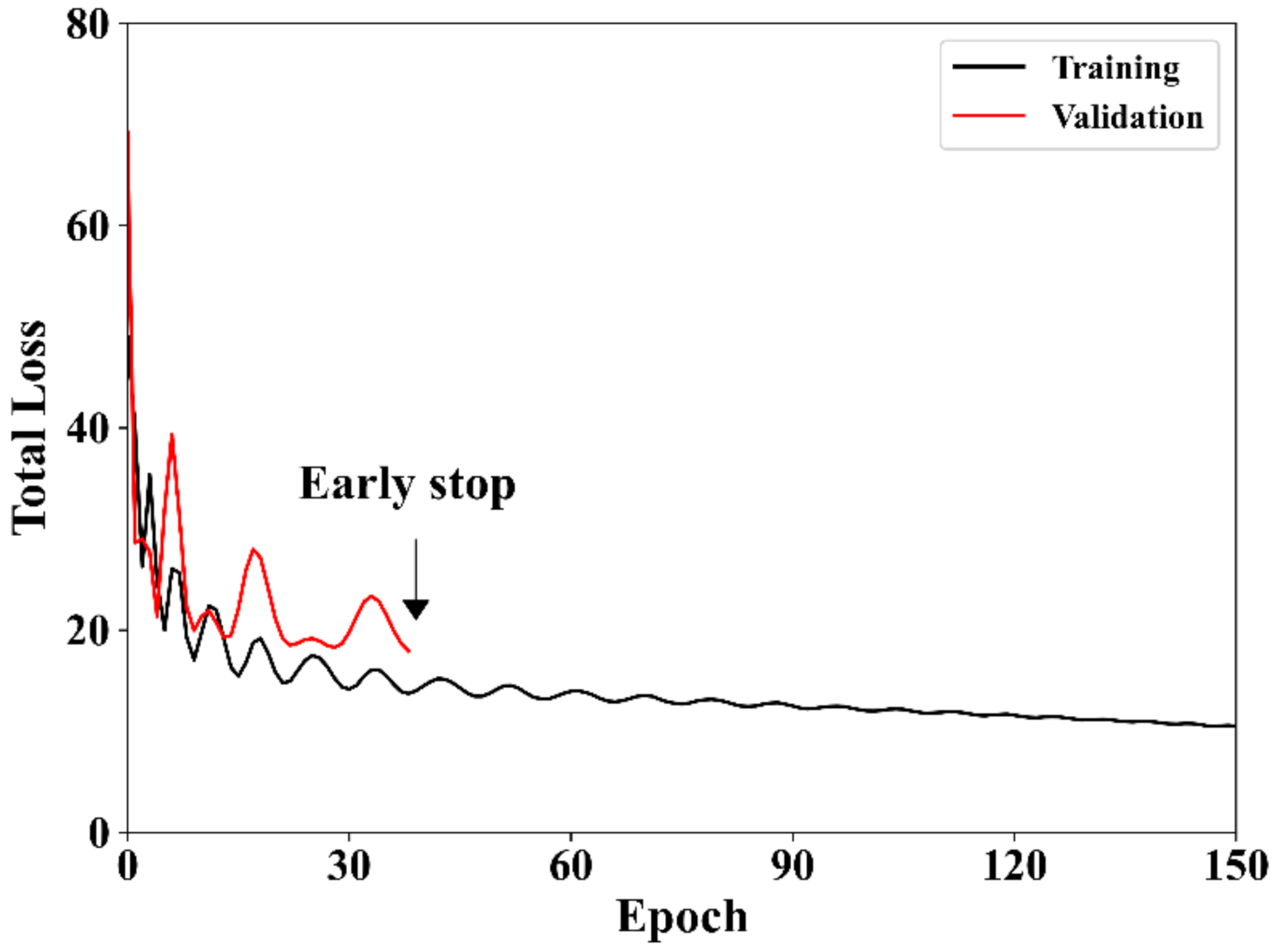
2.3. Model Optimization

The performance of machine learning algorithms depends heavily on identifying an appropriate set of hyperparameters, such as the depth of the convolutional blocks and the size and number of filters in the convolutional layers [50]. These parameters are sensitive to the features of the input data [32]. If the depth of these convolutional blocks becomes deeper, the number and weights of hyperparameters increase, which may lead to model overfitting. Conversely, if the depth of these blocks becomes shallower, this can lead to underfitting. Small filters in the model can capture more local features of the input image than large filters, whereas large filters are suitable for obtaining a general pattern of the input image. A small filter can extract a great deal of information from the input data but may require learning through a deeper convolutional layer because it slows down the rate at which the dimensions are reduced [32,51]. In the dropout layer, not all nodes in a neural network are trained; only part of the neural network is randomly trained. Hence, overfitting may be prevented due to the ensemble effect, thereby improving the model’s performance. Moreover, as the learning rate of the optimizer decreases, it is possible to finely train the model. This can also improve its performance but may lead to overfitting and increase the calculation time. Therefore, it is important to find the optimal hyperparameters for the features of the input data to obtain the best model performance.

In all our experiments, the hyperparameters in the validation dataset were tuned using the Keras tuner tool [52]. Specifically, the random search function of the Keras tuner tool was employed to find the optimal hyperparameters for the filter size of the convolutional layer, dropout rate of the dropout layer, and learning rate of the optimizer. As the number of random searches increases, the training time also increases. Thus, the appropriate range of hyperparameters for each scheme was determined before the tuning process (

Table 2. Ranges of the hyperparameters used to select the optimal values for the three convolutional neural network models using the Keras tuner tool.

Model	Layer	Size of the Selected Filter (Range)	Size of the Selected Dropout Rate (Range)	Size of the Selected Learning Rate (Range)
Scheme 1 (RMW)	Conv 1	7 (3, 5, 7, 9)	–	–
	Conv 2	9 (3, 5, 7, 9)	–	–
	Conv 3	7 (3, 5, 7, 9)	–	–
	Conv 4	9 (3, 5, 7, 9)	–	–
	Conv 5	7 (3, 5, 7, 9)	–	–
	Dropout	–	0.25 (0.25, 0.50, 0.75)	–
	Adam optimizer	–	–	10−6 (10−3, 10−4, 10−5, 10−6)
Scheme 1 (R34)	Conv 1	3 (3, 5, 7, 9)	–	–
	Conv 2	9 (3, 5, 7, 9)	–	–
	Conv 3	3 (3, 5, 7, 9)	–	–
	Conv 4	9 (3, 5, 7, 9)	–	–
	Conv 5	9 (3, 5, 7, 9)	–	–
	Dropout	–	0.25 (0.25, 0.50, 0.75)	–
	Adam optimizer	–	–	10−3 (10−3, 10−4, 10−5, 10−6)
Scheme 2	Conv 1	5 (3, 5, 7, 9)	–	–
	Conv 2	3 (3, 5, 7, 9)	–	–
	Conv 3	5 (3, 5, 7, 9)	–	–
	Conv 4	9 (3, 5, 7, 9)	–	–
	Conv 5	3 (3, 5, 7, 9)	–	–
	Dropout (RMW)	–	0.75 (0.25, 0.50, 0.75)	–
	Dropout (R34)	–	0.5 (0.25, 0.50, 0.75)	–
	Adam optimizer	–	–	10−4 (10−3, 10−4, 10−5, 10−6)
Scheme 3	Conv 1	5 (3, 5, 7, 9)	–	–
	Conv 2	9 (3, 5, 7, 9)	–	–
	Conv 3	5 (3, 5, 7, 9)	–	–
	Conv 4	7 (3, 5, 7, 9)	–	–
	Conv 5	9 (3, 5, 7, 9)	–	–
	Dropout (RMW)	–	0.5 (0.25, 0.50, 0.75)	–
	Dropout (R34)	–	0.75 (0.25, 0.50, 0.75)	–
	Adam optimizer	–	–	10−5 (10−3, 10−4, 10−5, 10−6)

). The filter size of the convolutional layer was set to increase in increments of two from 3 to 9. The dropout rates were set to 0.25, 0.50, and 0.75. For the optimizer, adaptive moment estimation (Adam) was used [53,54]. The optimizer plays a role in reducing the difference (i.e., loss) between the actual and predicted results. To find the optimal loss, the optimizer was transformed from gradient descent (GD) [55] into several forms, such as momentum [56], stochastic GD [57], adaptive gradient [58], adaptive delta [59], root mean square propagation [60], Nesterov accelerated gradient [61], Adam, AdaMax (a variant of Adam based on the infinity norm) [54], and Nesterov momentum into Adam [62], depending on the learning rate or direction. Among them, Adam appropriately considers both the direction and learning rate to find the optimal loss; therefore, it is fast, has good performance, and is consequently one of the most frequently used optimizers. To check the performance of the Adam optimizer, we performed sensitivity experiments using several optimizers provided by Keras and found that the Adam optimizer outperformed other optimizers. Additionally, four learning rate values (10⁻³, 10⁻⁴, 10⁻⁵, and 10⁻⁶) were tested to identify the optimal learning rate, in which the learning rate was defined as the initial learning rate × 1 ÷ (1 + decay × iteration). It should be noted that if the learning rate is too low, it will take a long time to find the optimal loss, while if it is too high, it may be impossible to find the optimal loss.

Early stopping is a method that informs when to stop running iterative algorithms during the training process, which improves the general performance of CNN models by reducing model overfitting and removing small test errors that are not visible during the training process [63,64]. The validation loss is the average model error of the validation data from a specified loss function, which tells the CNN model when to stop training. During the training process in this study, when the validation loss reached a minimum, the model training process was stopped (Figure 4).

2.4. Gradient-Weighted Class Activation Mapping

Deep learning methods, including CNNs, are widely referred to as “black boxes” because it is difficult to identify causal relationships between features extracted during training and output data using such methods [32]. To overcome this problem, a visualization method called gradient-weighted class activation mapping (Grad-CAM) [65] was used in this study. Unlike existing CAM methods [66], Grad-CAM does not need to replace the FC layer with global average pooling after the last convolutional layer. By not using global average pooling, stable heatmaps can be obtained in all layers without performance degradation. Based on Grad-CAM, heatmaps were extracted for the RMW and R34 models to understand the effect of each layer.

3. Results and Discussion

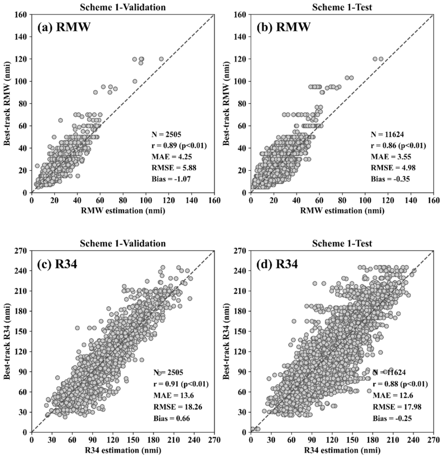
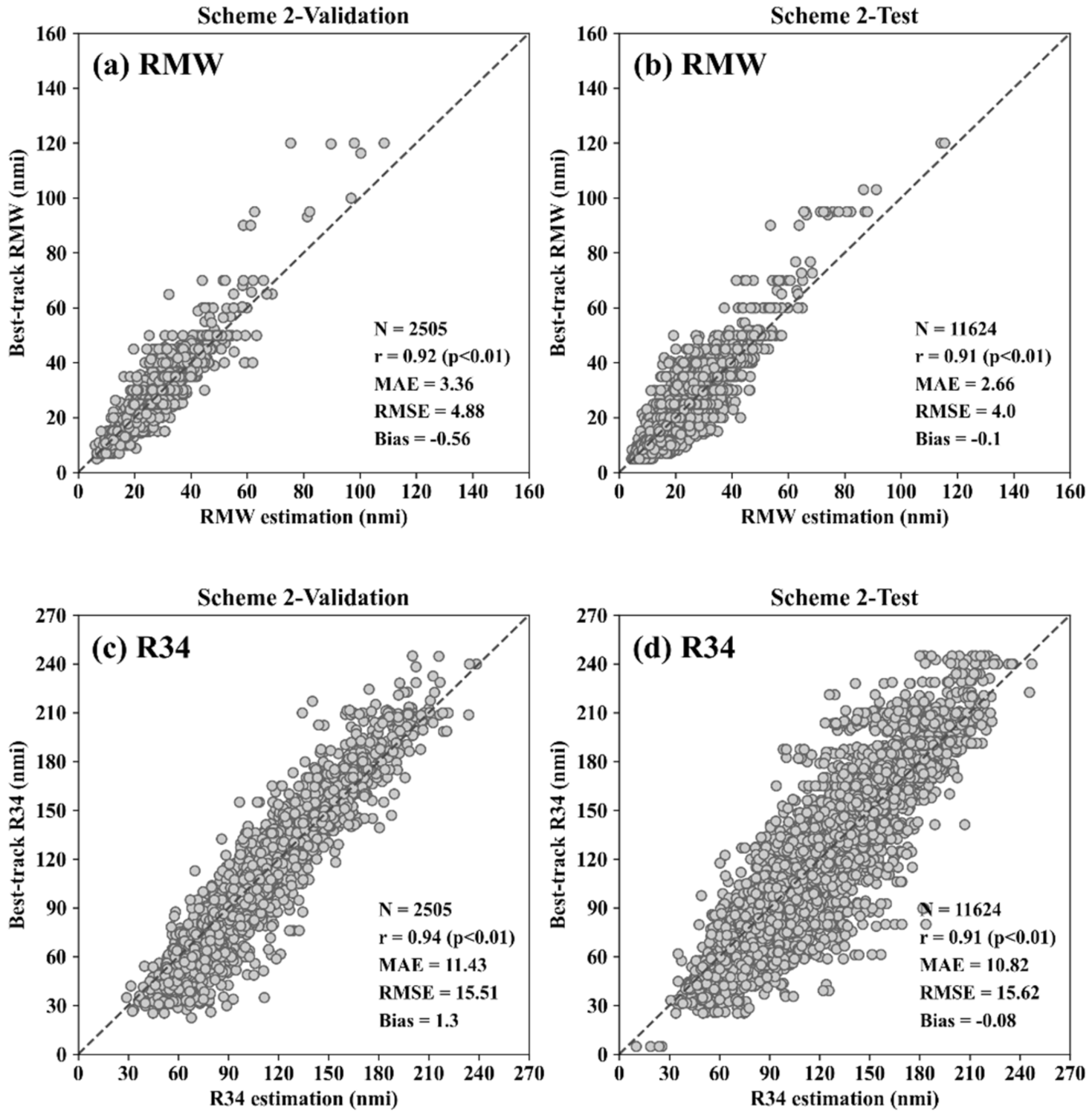
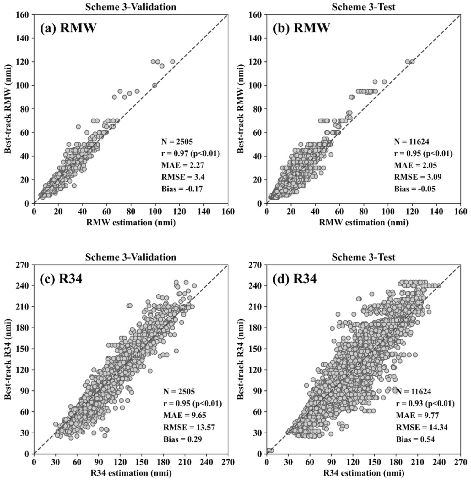
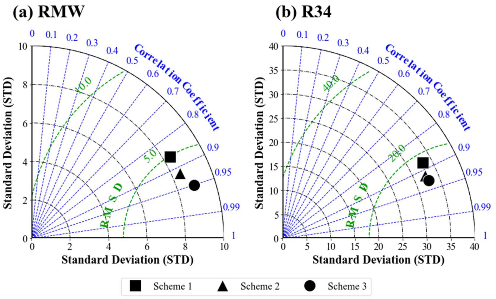
3.1. Performance of the Three CNN Schemes

This section describes the performance of the three CNN schemes that used 11,624 (test) and 2505 (validation) satellite images. The single-task TC-SEM (Scheme 1) obtained correlation coefficients (MAEs) of 0.89 (4.25 nmi) and 0.91 (13.6 nmi) for the RMW and R34, respectively (Figure 5a,c). When the optimized model using the validation results was applied to the test dataset, the correlation coefficients were 0.86 (3.55 nmi) and 0.88 (12.6 nmi), respectively (Figure 5b,d).

The validation and test results for the RMW showed negative biases for both (−1.07 and −0.35 nmi, respectively), indicating that the model tended to underestimate the RMW. The negative bias was greater when the RMW was greater than 60 nmi in the best track, which may have been related to insufficient data samples during training in this range (for example, samples over 60 nmi accounted for only 0.48% of the total). For R34, the validation and test results showed negative and positive biases, respectively. Thus, there was no consistent bias trend.

The simultaneous estimation of the RMW and R34 using the multi-task TC-SEM (Scheme 2) showed better validation performance for both the RMW and R34 (r = 0.92 and 0.94, MAE = 3.36 and 11.43 nmi, respectively; Figure 6a,c) compared with Scheme 1. Accordingly, the test results showed some improvement compared with Scheme 1 (r = 0.91 and 0.91, MAE = 2.66 and 10.82 nmi for the RMW and R34, respectively; Figure 6b,d). This may have been due to the inclusion of the features of both the RMW and R34 in the multi-task TC-SEM [47,48].

TC intensity was added to the multi-task model because it was expected that, since the intensity of a TC is generally related to its size, this information would improve the model’s performance. A significant negative correlation was found between TC intensity and the RMW (r = −0.67, p < 0.01), with the RMW tending to decrease as TC intensity increased (Figure 7a). There was also a statistically significant correlation between R34 and TC intensity (r = 0.44, p < 0.01; Figure 7b). As shown in Figure 8, the inclusion of TC intensity information in the multi-task model further improved the accuracy of the RMW and R34 estimations in the validation (r = 0.97 and 0.95, MAE = 2.27 and 9.65 nmi, respectively; Figure 8a,c). Accordingly, the test results of the RMW and R34 estimations using Scheme 3 (r = 0.95 and 0.93, respectively; MAE = 2.05 and 9.77 nmi, respectively; Figure 8b,d) were better than those of Scheme 2. Among the three schemes, the superiority of Scheme 3 in estimating TC size is also evident in the Taylor diagrams shown in Figure 9.

The results of this study were compared with those of previous studies based on existing wind radius estimation methods [14,20,23]. The findings revealed that the correlations and MAEs of our model were higher and lower, respectively, than those of previous studies for both the RMW and R34 (

Table 3. Comparison of the best-performing model in this study with other TC size estimation models in terms of the correlation and MAE. AO, WNP, and ENP represent the Atlantic Ocean, western North Pacific, and eastern North Pacific, respectively.

TC Size	Method	Region	Period Covered	Correlation	MAE (nmi)
RMW	Kossin et al. [23]	AO	1995–2004	0.58	13.11
	Scheme 3 (this study)	WNP	2011–2016	0.95	2.05
R34	Demuth et al. [14]	AO, ENP	1999–2004	0.89	16.90
	Knaff et al. [20]	AO, ENP	2011–2013	–	37.00
	Scheme 3 (this study)	WNP	2011–2016	0.93	9.77

). It should be noted that a direct quantitative comparison was not possible, as previous studies used different datasets. Nevertheless, given that our model’s accuracy in a large number of samples (11,624) spanning six years was comparable to or better than that of other operational products, our CNN model appears to be a powerful tool for estimating TC size.

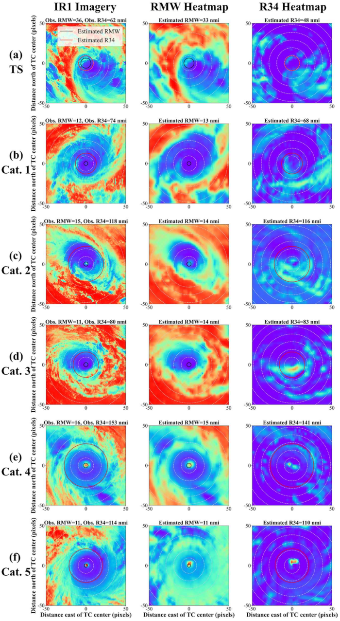
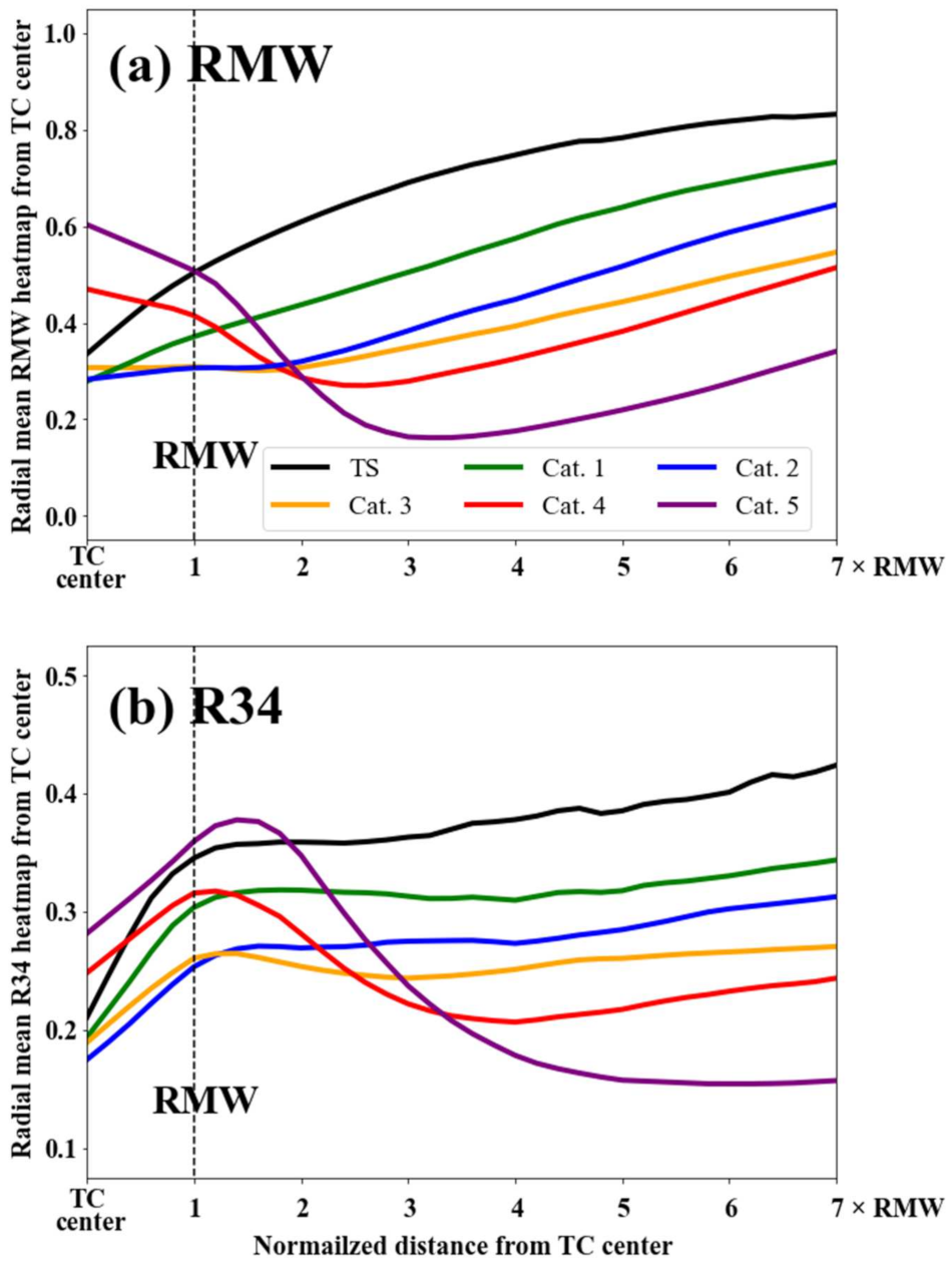
3.2. Class Activation Mapping

Figure 10 shows an example of heatmaps for the RMW and R34 calculated using Grad-CAM, along with COMS MI IR1 images, classified into six groups—tropical storms (TS) and category 1–5 TCs according to the Saffir–Simpson Hurricane Wind Scale. In the satellite images, it can be seen that the stronger the intensity, the more pronounced the TC eye. Thus, when the TC eye was distinct (category 4 and 5 TCs; Figure 10e,f), the TC-SEM seemed to estimate the RMW mainly using information from around the TC eye. These patterns can be clearly seen in the radial-averaged heatmap estimated using all TCs in the same intensity group (Figure 11a) in which the eyes of category 4 and 5 TCs had high heatmap values. Considering that the maximum wind speed (Vmax) of a TC is usually located near the eyewall that surrounds the eye of the TC, information from around the TC eye is clearly useful for determining the RMW. On the other hand, for TCs of weak-to-medium intensity (categories 1–3; Figure 10a–d and Figure 11a), the heatmap values were greater toward the outside regions of the TCs than toward their centers, as the eyes of these TCs were not clear in the satellite images.

For R34, the overall pattern was similar to that of the RMW, except that as the TC became stronger, the heatmap values were higher near the RMW than near the TC eye region (Figure 11b). Unlike the RMW, for relatively weaker TCs (categories 1–3), the heatmap values were almost equally high from the RMW to regions outside the TC. The rate of decline (i.e., slope) from the Vmax to the outer weak wind speed was an important factor for determining the R34, as shown in Figure 2. This is why the TC-SEM used all the information from the RMW to the outside region of the TC equally to determine the R34, especially for weaker TC regions (Figure 11b).

3.3. Sensitivity Test of Dropout and Pooling Layers

Previous research indicated that the use of dropout layers in CNN models for intensity estimation may increase the model error [33]. Therefore, we performed a sensitivity experiment to investigate whether removing the dropout layers (Figure 3) could reduce the errors in estimating the RMW and R34 in Schemes 1, 2, and 3.

The results showed that removing the dropout layers improved the performance of Schemes 1 and 2, while retaining them improved the performance of Scheme 3 (

Table 4. Validation and testing results for the three CNN-based TC size estimation models with and without dropout layers. The model with the best validation and testing accuracy is denoted in bold. The asterisks (*) indicate statistical significance at the 99% confidence level based on Student’s t-test.

Model		RWW				R34
		Corr.	RMSE (nmi)	MAE (nmi)	Bias (nmi)	Corr.	RMSE (nmi)	MAE (nmi)	Bias (nmi)
With dropout layers	Scheme 1	0.89 * (0.86 *)	5.88 (4.98)	4.25 (3.55)	−1.07 (−0.35)	0.91 * (0.88 *)	18.26 (17.98)	13.60 (12.60)	0.66 (−0.25)
	Scheme 2	0.92 * (0.91 *)	4.88 (4.00)	3.36 (2.66)	−0.56 (−0.10)	0.94 * (0.91 *)	15.51 (15.62)	11.43 (10.82)	1.30 (−0.08)
	Scheme 3	0.97 * (0.95 *)	3.40 (3.09)	2.27 (2.05)	−0.17 (−0.05)	0.95 * (0.93 *)	13.57 (14.34)	9.65 (9.77)	0.29 (0.54)
Without dropout layers	Scheme 1	0.93 * (0.92 *)	4.83 (4.04)	3.29 (2.66)	−1.06 (−0.41)	0.93 * (0.90 *)	15.77 (16.75)	11.46 (11.54)	1.42 (0.12)
	Scheme 2	0.94 * (0.92 *)	4.45 (3.80)	2.97 (2.48)	−0.92 (−0.31)	0.94 * (0.91 *)	15.72 (16.23)	11.42 (11.19)	0.88 (−0.45)
	Scheme 3	0.95 * (0.93 *)	4.16 (3.64)	2.90 (2.50)	−0.13 (−0.12)	0.94 * (0.92 *)	15.11 (15.26)	11.11 (10.82)	−0.12 (−0.18)

). This suggests that the TC size estimation model was sensitive to the dropout layer, as was the TC intensity estimation model, and that the effect of the dropout layer depended on how the CNN model was constructed.

Pooling techniques or pooling layers are commonly used in CNN models to reduce computational complexity by storing representative values of a group of features instead of the original values [33,67,68]. However, the fine structural features of TCs can be removed during the pooling process [33]. In this study, due to limited computing resources, pooling layers were used to increase the number of filters containing TC features.

4. Summary and Conclusions

This study proposed a novel TC-SEM based on a CNN model and geostationary satellite images of four IR channels obtained from the WNP. The TC-SEM was trained, validated, and tested to estimate the RMW and R34 of TCs using 43,859 satellite images and TC best-track data. The multi-task model that estimated the RMW and R34 simultaneously and used additional TC intensity information showed the best performance. This suggests that the accuracy of the TC-SEM could be improved by knowledge sharing while simultaneously performing multiple interrelated tasks and by using additional useful information. Based on Grad-CAM, heatmaps were created to understand what areas of TCs the model used when estimating the RMW and R34. The analysis showed that the areas differed depending on TC intensity. For weak TCs, the model mainly used information from the outer regions, whereas for strong TCs, it used information from the TC eye and eyewalls. A comparison with previous studies showed that the accuracy of our model was comparable to or better than that of existing methods.

Existing TC size estimation methods consist of direct estimations using scatterometry data and indirect estimations using geostationary satellite IR images. In the former case, the RMW—the inner core of a TC—cannot be accurately estimated due to the low spatial resolution of scatterometry; in the latter case, the RMW and R34 estimations have low accuracy in the absence of a discernable TC eye and in the case of weak TCs because they use empirical linear regression that depends on climate information. Although this study did not compare the accuracy of the proposed model with existing methods on the same sample, the overall high accuracy achieved suggests that our model using artificial intelligence technology could be an alternative method for estimating TC size that is relatively reliable and accurate in all cases, with and without discernable TC eyes.

This is the first study to estimate TC size by applying multichannel IR images to a CNN model, suggesting that this new method can be a powerful tool for estimating TC size in operational TC predictions. However, since TC intensity information from best-track data is not provided in real time, TC warning centers may use the TC-SEM after estimating a TC’s intensity. In this case, the performance of the TC-SEM may deteriorate due to errors in the estimation of TC intensity. Whether to use the TC intensity estimated via the TC-SEM will depend on the accuracy of the TC intensity estimation. In addition to the intensity information, the TC-SEM can be further improved by including additional environmental variables related to TC size. This, however, requires further investigation.

In this study, asymmetric characteristics of TC size were not considered. Such information is important for more accurate predictions of TC-related hazardous areas [69,70,71]. As best-track data contain asymmetric TC size information, such as wind radii on the longest/shortest axis or quadrant, the TC-SEM can be used in future studies to estimate asymmetric TC sizes.

References

1. Chavas, D.R.; Lin, N.; Emanuel, K. A model for the complete radial structure of the tropical cyclone wind field. Part I: Comparison with observed structure. J. Atmos. Sci. 2015, 72, 3647–3662. [Google Scholar] [CrossRef]
2. Kimball, S.K.; Mulekar, M.S. A 15-year climatology of North Atlantic tropical cyclones. Part I: Size parameters. J. Clim. 2004, 17, 3555–3575. [Google Scholar] [CrossRef]
3. Moyer, A.C.; Evans, J.L.; Powell, M. Comparison of observed gale radius statistics. Meteorol. Atmos. Phys. 2007, 97, 41–55. [Google Scholar] [CrossRef]
4. Merrill, R.T. A comparison of large and small tropical cyclones. Mon. Weather Rev. 1984, 112, 1408–1418. [Google Scholar] [CrossRef] [Green Version]
5. Weatherford, C.L.; Gray, W.M. Typhoon structure as revealed by aircraft reconnaissance. Part I: Data analysis and climatology. Mon. Weather Rev. 1988, 116, 1032–1043. [Google Scholar] [CrossRef] [Green Version]
6. Maclay, K.S.; DeMaria, M.; Vonder Haar, T.H. Tropical cyclone inner-core kinetic energy evolution. Mon. Weather Rev. 2008, 136, 4882–4898. [Google Scholar] [CrossRef] [Green Version]
7. Knaff, J.A.; Sampson, C.R.; DeMaria, M.; Marchok, T.P.; Gross, J.M.; McAdie, C.J. Statistical tropical cyclone wind radii prediction using climatology and persistence. Weather Forecast. 2007, 22, 781–791. [Google Scholar] [CrossRef]
8. Knaff, J.A.; Sampson, C.R. After a decade are Atlantic tropical cyclone gale force wind radii forecasts now skillful? Weather Forecast. 2015, 30, 702–709. [Google Scholar] [CrossRef]
9. Chan, K.T.; Chan, J.C. Impacts of initial vortex size and planetary vorticity on tropical cyclone size. Q. J. R. Meteorol. Soc. 2014, 140, 2235–2248. [Google Scholar] [CrossRef]
10. Chan, K.T.; Chan, J.C. Global climatology of tropical cyclone size as inferred from QuikSCAT data. Int. J. Clim. 2015, 35, 4843–4848. [Google Scholar] [CrossRef]
11. Wu, L.; Tian, W.; Liu, Q.; Cao, J.; Knaff, J.A. Implications of the observed relationship between tropical cyclone size and intensity over the western North Pacific. J. Clim. 2015, 28, 9501–9506. [Google Scholar] [CrossRef]
12. Brennan, M.J.; Hennon, C.C.; Knabb, R.D. The operational use of QuikSCAT ocean surface vector winds at the National Hurricane Center. Weather Forecast. 2009, 24, 621–645. [Google Scholar] [CrossRef] [Green Version]
13. Demuth, J.L.; DeMaria, M.; Knaff, J.A.; Vonder Haar, T.H. Evaluation of Advanced Microwave Sounding Unit tropical-cyclone intensity and size estimation algorithms. J. Appl. Meteorol. 2004, 43, 282–296. [Google Scholar] [CrossRef] [Green Version]
14. Demuth, J.L.; DeMaria, M.; Knaff, J.A. Improvement of Advanced Microwave Sounding Unit tropical cyclone intensity and size estimation algorithms. J. Appl. Meteorol. Climatol. 2006, 45, 1573–1581. [Google Scholar] [CrossRef]
15. Hsu, S.A.; Babin, A. Estimating the radius of maximum wind via satellite during Hurricane Lili (2002) over the Gulf of Mexico. Natl. Weather Assoc. Electron. J. 2005, 6, 1–6. [Google Scholar]
16. Mueller, K.J.; DeMaria, M.; Knaff, J.; Kossin, J.P.; Vonder Haar, T.H. Objective estimation of tropical cyclone wind structure from infrared satellite data. Weather Forecast. 2006, 21, 990–1005. [Google Scholar] [CrossRef] [Green Version]
17. Kwon, M. Estimation and statistical characteristics of the radius of maximum wind of tropical cyclones using COMS IR imagery. Atmosphere 2012, 22, 473–481. (In Korean) [Google Scholar] [CrossRef] [Green Version]
18. Lee, Y.K.; Kwon, M. An Estimation of the of Tropical Cyclone Size Using COMS Infrared Imagery. Atmosphere 2015, 25, 569–573. (In Korean) [Google Scholar] [CrossRef] [Green Version]
19. Knaff, J.A.; Longmore, S.P.; DeMaria, R.T.; Molenar, D.A. Improved tropical-cyclone flight-level wind estimates using routine infrared satellite reconnaissance. J. Appl. Meteorol. Climatol. 2015, 54, 463–478. [Google Scholar] [CrossRef] [Green Version]
20. Knaff, J.A.; Slocum, C.J.; Musgrave, K.D.; Sampson, C.R.; Strahl, B.R. Using routinely available information to estimate tropical cyclone wind structure. Mon. Weather Rev. 2016, 144, 1233–1247. [Google Scholar] [CrossRef]
21. Olander, T.L.; Velden, C.S. ADT-Advanced Dvorak Technique User’s Guide; University of Wisconsin-Madison: Madison, WI, USA, 2015. [Google Scholar]
22. Knaff, J.A.; Harper, B.A. KN1: Tropical cyclone surface wind structure and wind-pressure relationships. In Proceedings of the WMO Seventh International Workshop on Tropical Cyclones, La Reunion, France, 15–20 November 2010; p. 35. [Google Scholar]
23. Kossin, J.P.; Knaff, J.A.; Berger, H.I.; Herndon, D.C.; Cram, T.A.; Velden, C.S.; Murnane, R.J.; Hawkins, J.D. Estimating hurricane wind structure in the absence of aircraft reconnaissance. Weather Forecast. 2007, 22, 89–101. [Google Scholar] [CrossRef]
24. Bentamy, A.; Croize-Fillon, D.; Perigaud, C. Characterization of ASCAT measurements based on buoy and QuikSCAT wind vector observations. Ocean Sci. 2008, 4, 265–274. [Google Scholar] [CrossRef] [Green Version]
25. Knaff, J.A.; DeMaria, M.; Molenar, D.A.; Sampson, C.R.; Seybold, M.G. An automated, objective, multiple-satellite-platform tropical cyclone surface wind analysis. J. Appl. Meteorol. Clim. 2011, 50, 2149–2166. [Google Scholar] [CrossRef] [Green Version]
26. Hong, S.; Shin, I. Wind speed retrieval based on sea surface roughness measurements from spaceborne microwave radiometers. J. Appl. Meteorol. Clim. 2013, 52, 507–516. [Google Scholar] [CrossRef]
27. Muroi, C. Brief History and recent activities of RSMC Tokyo-Typhoon Centre. Trop. Cyclone Res. Rev. 2018, 7, 57–64. [Google Scholar]
28. Simonyan, K.; Zisserman, A. Very deep convolutional networks for large-scale image recognition. In Proceedings of the ICLR 2015, San Diego, CA, USA, 7–9 May 2015. [Google Scholar]
29. Pradhan, R.; Aygun, R.S.; Maskey, M.; Ramachandran, R.; Cecil, D.J. Tropical cyclone intensity estimation using a deep convolutional neural network. IEEE Trans. Image Process. 2018, 27, 692–702. [Google Scholar] [CrossRef] [PubMed]
30. Combinido, J.S.; Mendoza, J.R.; Aborot, J. A Convolutional Neural Network Approach for Estimating Tropical Cyclone Intensity Using Satellite-based Infrared Images. In Proceedings of the 2018 24th ICPR, Beijing, China, 20–24 August 2018. [Google Scholar]
31. Wimmers, A.; Velden, C.; Cossuth, J.H. Using deep learning to estimate tropical cyclone intensity from satellite passive microwave imagery. Mon. Weather Rev. 2019, 147, 2261–2282. [Google Scholar] [CrossRef]
32. Lee, J.; Im, J.; Cha, D.H.; Park, H.; Sim, S. Tropical cyclone intensity estimation using multi-dimensional convolutional neural networks from geostationary satellite data. Remote Sens. 2019, 12, 108. [Google Scholar] [CrossRef] [Green Version]
33. Chen, B.F.; Chen, B.; Lin, H.T.; Elsberry, R.L. Estimating tropical cyclone intensity by satellite imagery utilizing convolutional neural networks. Weather Forecast. 2019, 34, 447–465. [Google Scholar]
34. Tian, W.; Huang, W.; Yi, L.; Wu, L.; Wang, C. A CNN-Based Hybrid Model for Tropical Cyclone Intensity Estimation in Meteorological Industry. IEEE Access 2020, 8, 59158–59168. [Google Scholar] [CrossRef]
35. Wang, X.; Wang, W.; Yan, B. Tropical Cyclone Intensity Change Prediction Based on Surrounding Environmental Conditions with Deep Learning. Water 2020, 12, 2685. [Google Scholar] [CrossRef]
36. Wang, C.; Xu, Q.; Li, X.; Cheng, Y. CNN-Based Tropical Cyclone Track Forecasting from Satellite Infrared Images. In IGARSS 2020—2020 IEEE International Geoscience and Remote Sensing Symposium; IEEE: Piscataway, NJ, USA, 2020; pp. 5811–5814. [Google Scholar]
37. Ou, M.L.; Won, J.-K. Introduction to the COMS Program and its application to meteorological services of Korea. In Proceedings of the 2005 EUMETSAT Meteorological Satellite Conference, Dubrovnik, Croatia, 19–23 September 2005; pp. 19–23. [Google Scholar]
38. Schmetz, J.; Tjemkes, S.A.; Gube, M.; Van de Berg, L. Monitoring deep convection and convective overshooting with METEOSAT. Adv. Space Res. 1997, 19, 433–441. [Google Scholar] [CrossRef]
39. Velden, C.S.; Hayden, C.M.; Nieman, S.J.W.; Paul Menzel, W.; Wanzong, S.; Goerss, J.S. Upper-tropospheric winds derived from geostationary satellite water vapor observations. Bull. Am. Meteorol. Soc. 1997, 78, 173–195. [Google Scholar] [CrossRef] [Green Version]
40. Ralph, F.M.; Neiman, P.J.; Wick, G.A. Satellite and CALJET aircraft observations of atmospheric rivers over the eastern North Pacific Ocean during the winter of 1997/98. Mon. Weather Rev. 2004, 132, 1721–1745. [Google Scholar] [CrossRef] [Green Version]
41. Durry, G.; Amarouche, N.; Zéninari, V.; Parvitte, B.; Lebarbu, T.; Ovarlez, J. In situ sensing of the middle atmosphere with balloonborne near-infrared laser diodes. Spectrochim. Acta Part A 2004, 60, 3371–3379. [Google Scholar] [CrossRef]
42. Kruk, M.C.; Knapp, K.R.; Levinson, D.H.; Diamond, H.J.; Kossin, J.P. An Overview of the International Best Track Archive for Climate Stewardship (IBTrACS). In Proceedings of the 21st Conference on Climate Variability and Change, Phoenix, AZ, USA, 11–15 January 2010. 7B.1. [Google Scholar]
43. Knapp, K.R.; Kruk, M.C.; Levinson, D.H.; Diamond, H.J.; Neumann, C.J. The International Best Track Archive for Climate Stewardship (IBTrACS). Bull. Am. Meteorol. Soc. 2010, 91, 363–376. [Google Scholar] [CrossRef]
44. Glorot, X.; Bengio, Y. Understanding the difficulty of training deep feedforward neural networks. In Proceedings of the Thirteenth International Conference on Artificial Intelligence and Statistics, Sardinia, Italy, 13–15 May 2010; pp. 249–256. [Google Scholar]
45. Tensorflow. Available online: https://www.tensorflow.org/api_docs/python/tf/keras/initializers/GlorotUniform/ (accessed on 15 December 2021).
46. Arnekvist, I.; Carvalho, J.F.; Kragic, D.; Stork, J.A. The effect of target normalization and momentum on dying relu. arXiv 2020, arXiv:2005.06195. [Google Scholar]
47. Abdulnabi, A.H.; Wang, G.; Lu, J.; Jia, K. Multi-task CNN model for attribute prediction. IEEE Trans. Multimed. 2015, 17, 1949–1959. [Google Scholar] [CrossRef] [Green Version]
48. Caruana, R. Multitask learning. Mach. Learn. 1997, 28, 41–75. [Google Scholar] [CrossRef]
49. Abadi, M.; Barham, P.; Chen, J.; Chen, Z.; Davis, A.; Dean, J.; Devin, M.; Ghemawat, S.; Irving, G.; Isard, M.; et al. Tensorflow: A system for large-scale machine learning. In Proceedings of the 12th {USENIX} Symposium on Operating Systems Design and Implementation (OSDI’16), Savannah, GA, USA, 2–4 November 2016; pp. 265–283. [Google Scholar]
50. Li, L.; Jamieson, K.; DeSalvo, G.; Rostamizadeh, A.; Talwalkar, A. Hyperband: A novel bandit-based approach to hyperparameter optimization. J. Mach. Learn. Res. 2017, 18, 6765–6816. [Google Scholar]
51. LeCun, Y.; Boser, B.; Denker, J.S.; Henderson, D.; Howard, R.E.; Hubbard, W.; Jackel, L.D. Handwritten digit recognition with a back-propagation network. In Advances in Neural Information Processing Systems; MIT Press: Cambridge, MA, USA, 1989; pp. 396–404. [Google Scholar]
52. Keras Tuner. Available online: https://keras-team.github.io/keras-tuner/ (accessed on 30 October 2021).
53. Nair, V.; Hinton, G.E. Rectified linear units improve restricted boltzmann machines. In Proceedings of the 27th International Conference on Machine Learning (ICML), Haifa, Israel, 21–24 June 2010. [Google Scholar]
54. Kingma, D.P.; Ba, J. Adam: A method for stochastic optimization. arXiv 2015, arXiv:1412.6980. [Google Scholar]
55. Cauchy, A. Méthode générale pour la résolution des systemes d’équations simultanées. Comp. Rend. Sci. 1847, 25, 536–538. [Google Scholar]
56. Polyak, B.T. Some methods of speeding up the convergence of iteration methods. USSR Comput. Math. Math. Phys. 1964, 4, 1–17. [Google Scholar] [CrossRef]
57. Nemirovski, A.; Juditsky, A.; Lan, G.; Shapiro, A. Robust stochastic approximation approach to stochastic programming. SIAM J. Optim. 2009, 19, 1574–1609. [Google Scholar] [CrossRef] [Green Version]
58. Duchi, J.; Hazan, E.; Singer, Y. Adaptive subgradient methods for online learning and stochastic optimization. J. Mach. Learn. Res. 2011, 12, 2121–2159. [Google Scholar]
59. Zeiler, M.D. Adadelta: An adaptive learning rate method. arXiv 2012, arXiv:1212.5701. [Google Scholar]
60. Hinton, G.E. A practical guide to training restricted Boltzmann machines. In Neural Networks: Tricks of the Trade; Springer: Berlin/Heidelberg, Germany, 2012; pp. 599–619. [Google Scholar]
61. Sutskever, I.; Martens, J.; Dahl, G.; Hinton, G. On the importance of initialization and momentum in deep learning. In Proceedings of the 30th International Conference on Machine Learning, Atlanta, GA, USA, 16–21 June 2013; pp. 1139–1147. [Google Scholar]
62. Dozat, T. Incorporating Nesterov Momentum into Adam. In Proceedings of the 4th International Conference on Learning Prepresentations (ICLR), San Juan, Puerto Rico, 2–4 May 2016. [Google Scholar]
63. Raskutti, G.; Wainwright, M.J.; Yu, B. Early stopping and non-parametric regression: An optimal data-dependent stopping rule. J. Mach. Learn. Res. 2014, 15, 335–366. [Google Scholar]
64. Chi, J.; Li, X.; Wang, H.; Gao, D.; Gerstoft, P. Sound source ranging using a feed-forward neural network trained with fitting-based early stopping. J. Acoust. Soc. Am. 2019, 146, EL258–EL264. [Google Scholar] [CrossRef] [Green Version]
65. Selvaraju, R.R.; Cogswell, M.; Das, A.; Vedantam, R.; Parikh, D.; Batra, D. Grad-cam: Visual explanations from deep networks via gradient-based localization. In Proceedings of the IEEE International Conference on Computer Vision, Venice, Italy, 22–29 October 2017; pp. 618–626. [Google Scholar]
66. Zhou, B.; Khosla, A.; Lapedriza, A.; Oliva, A.; Torralba, A. Learning deep features for discriminative localization. In Proceedings of the IEEE Conference on Computer Vision and Pattern Recognition, Las Vegas, NV, USA, 27–30 June 2016; pp. 2921–2929. [Google Scholar]
67. Krizhevsky, A.; Sutskever, I.; Hinton, G.E. Imagenet classification with deep convolutional neural networks. Adv. Neural Inf. Process. Syst. 2012, 25, 1097–1105. [Google Scholar] [CrossRef]
68. Zhang, P.; Ke, Y.; Zhang, Z.; Wang, M.; Li, P.; Zhang, S. Urban land use and land cover classification using novel deep learning models based on high spatial resolution satellite imagery. Sensors 2018, 18, 3717. [Google Scholar] [CrossRef] [PubMed] [Green Version]
69. Reasor, P.D.; Montgomery, M.T.; Grasso, L.D. A new look at the problem of tropical cyclones in vertical shear flow: Vortex resiliency. J. Atmos. Sci. 2004, 61, 3–22. [Google Scholar] [CrossRef] [Green Version]
70. Sampson, C.R.; Wittmann, P.A.; Tolman, H.L. Consistent tropical cyclone wind and wave forecasts for the US Navy. Weather Forecast. 2010, 25, 1293–1306. [Google Scholar] [CrossRef]
71. Lazarus, S.M.; Wilson, S.T.; Splitt, M.E.; Zarillo, G.A. Evaluation of a wind-wave system for ensemble tropical cyclone wave forecasting. Part I: Winds. Weather Forecast. 2013, 28, 297–315. [Google Scholar] [CrossRef] [Green Version]
Figure 1. Examples of normalized brightness temperature images of a radius of about 600 km from the center of Typhoon Meranti (1614) extracted from the (a) infrared 1 (IR1), (b) infrared 2 (IR2), (c) water vapor (WV), and (d) short-wavelength infrared (SWIR) channels of the COMS Meteorological Imager. The images were obtained at 12:00 UTC on September 13, 2016 (location: 123.0923° E, 20.3716° N). The axis units are pixels (1 pixel = ~12 km).
Remotesensing 14 00426 g001
Figure 2. Schematic diagram of the radius of maximum wind (RMW; dashed red line) and 34 kt wind (R34; dashed green line) of Typhoon Rammasun (0308). The radial profile was obtained from QuikSCAT at 20:42 UTC on 9 May 2008. VMAX represents the maximum wind speed. At TC warning centers, the wind speed and distances from the TC center (including the RMW and R34) are reported in knots (1 kt = 0.514 m s−1) and nautical miles (1 nmi = 0.185 km), respectively. For this reason, these operational units are used exclusively hereafter.
Remotesensing 14 00426 g002
Figure 3. The architecture of the three CNN models used in this study: (a) a single-task model (Scheme 1), (b) a multi-task model (Scheme 2), and (c) a multi-task model using additional TC intensity information as input (Scheme 3). The numbers in parentheses indicate the number of filters, max pooling size, activation function, or data size in each layer.
Remotesensing 14 00426 g003
Figure 4. Schematic diagram of training loss (black line) and validation loss (red line) for the number of epochs (1 epoch = [training set size ÷ batch size] × iterations). As the epochs progressed, the training loss continuously decreased and converged to zero, while the validation loss increased or became constant in a specific epoch (i.e., overfitting). Training was stopped early in the epoch in which the minimum (or constant) validation loss appeared to prevent overfitting.
Remotesensing 14 00426 g004
Figure 5. Validation (a,c) and test (b,d) results of the RMW and R34 estimated using the single-task model (Scheme 1). In each panel, the x-axis shows the RMW and R34 predicted by the model, and the y-axis shows the best-track RMW and R34 data. The validation data were used only to optimize the proposed model and were independent of the test data. The number of samples (N), correlation coefficient (r) and p-value, mean absolute error (MAE), root mean square error (RMSE), and bias are presented in the bottom-right corner of each panel.
Remotesensing 14 00426 g005
Figure 6. The same as Figure 5, but these were estimated using the multi-task model (Scheme 2).
Remotesensing 14 00426 g006
Figure 7. Relationship between TC intensity and (a) RMW and (b) R34. The different colors represent the density of the data estimated using the Gaussian kernel function. The number of samples (N), correlation coefficient, root mean square error (RMSE), and bias are also shown.
Remotesensing 14 00426 g007
Figure 8. The same as Figure 5, but these were estimated using the multi-task model with additional TC intensity information (Scheme 3).
Remotesensing 14 00426 g008
Figure 9. Taylor diagrams for (a) the RMW and (b) the R34 comparing the results of the three schemes.
Remotesensing 14 00426 g009
Figure 10. Examples of COMS Meteorological Imager infrared 1 (IR1) images (left panels), heatmaps of the radius of maximum wind (RMW) (center panels), and radius of 34 kt wind (R34) (right panels) calculated using a gradient-weighted class activation mapping (Grad-CAM) for tropical cyclones (TCs) based on the Saffir–Simpson Hurricane Wind Scale. (a) Tropical storm (TS) and category (b) 1, (c) 2, (d) 3, (e) 4, and (f) 5 TCs. The solid black and red circles represent the RMW and R34, respectively, which were estimated using the TC-SEM proposed in this study. The images were randomly selected according to TC intensity. The axis units are pixels (1 pixel = ~12 km).
Remotesensing 14 00426 g010
Figure 11. Radial mean heatmaps from the center of the tropical cyclone (TC) for (a) the radius of maximum wind (RMW) and (b) the radius of 34 kt wind (R34) estimated for TCs of each category on the Saffir–Simpson Hurricane Wind Scale. The x-axis is the distance normalized by the RMW (i.e., 1 is the RMW, 2 is twice the RMW, etc.).
Remotesensing 14 00426 g011