
Estimating Boundary Layer Height from LiDAR Data under Complex Atmospheric Conditions Using Machine Learning


Abstract
:1. Introduction
2. Materials
2.1. Micro-Pulse LiDAR (MPL)
2.2. Radiosonde (RS)
3. Methods
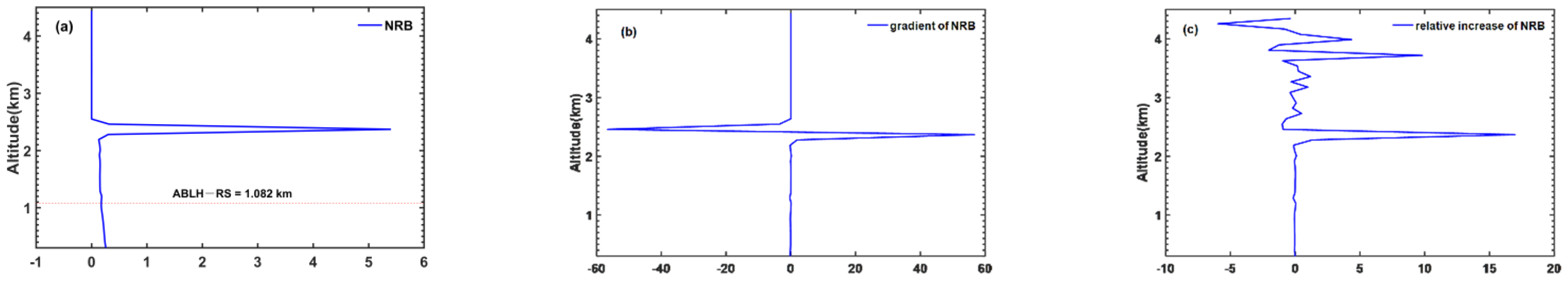
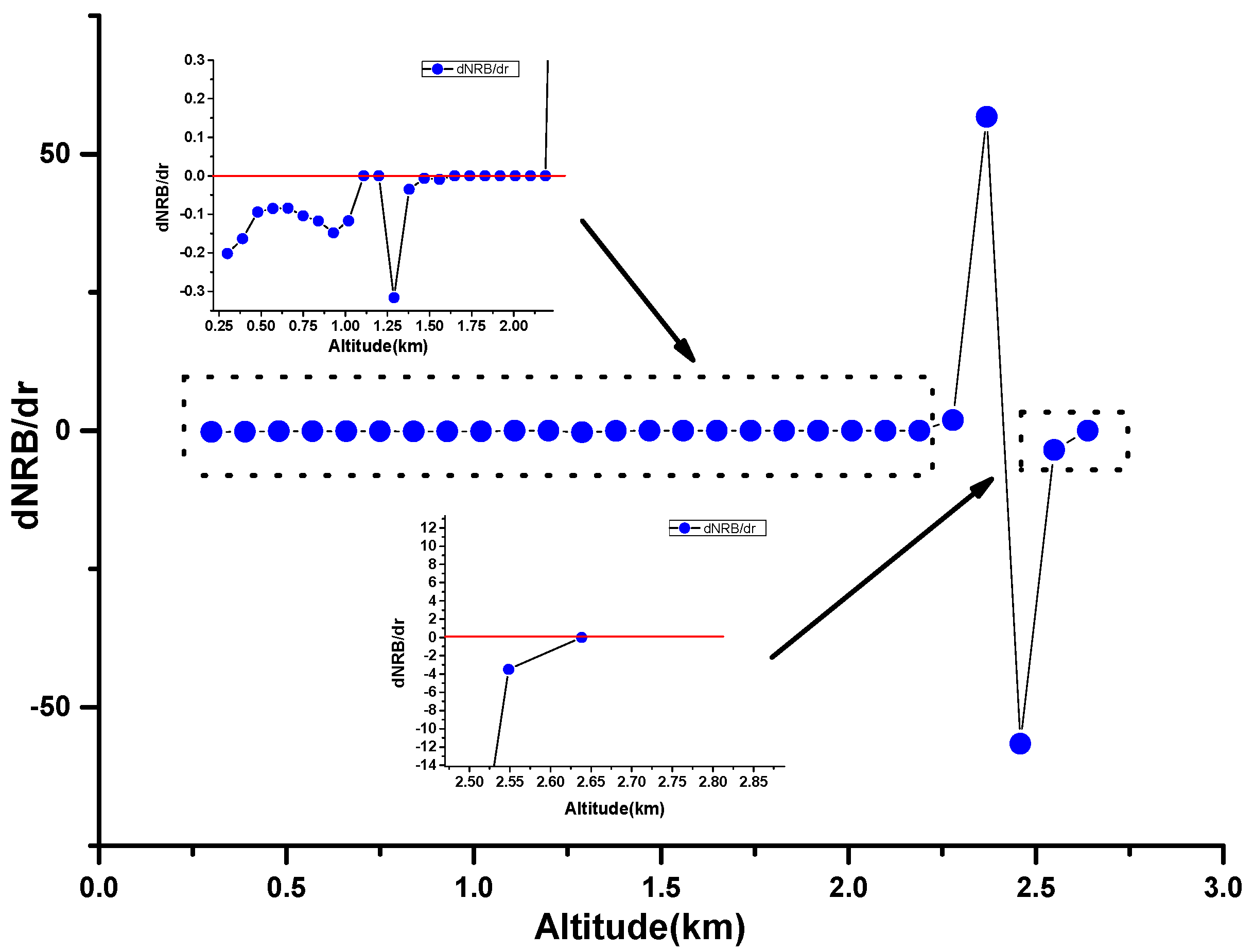
3.1. Gradient Method (GM)
3.2. Wavelet Covariance Transform Method (WM)
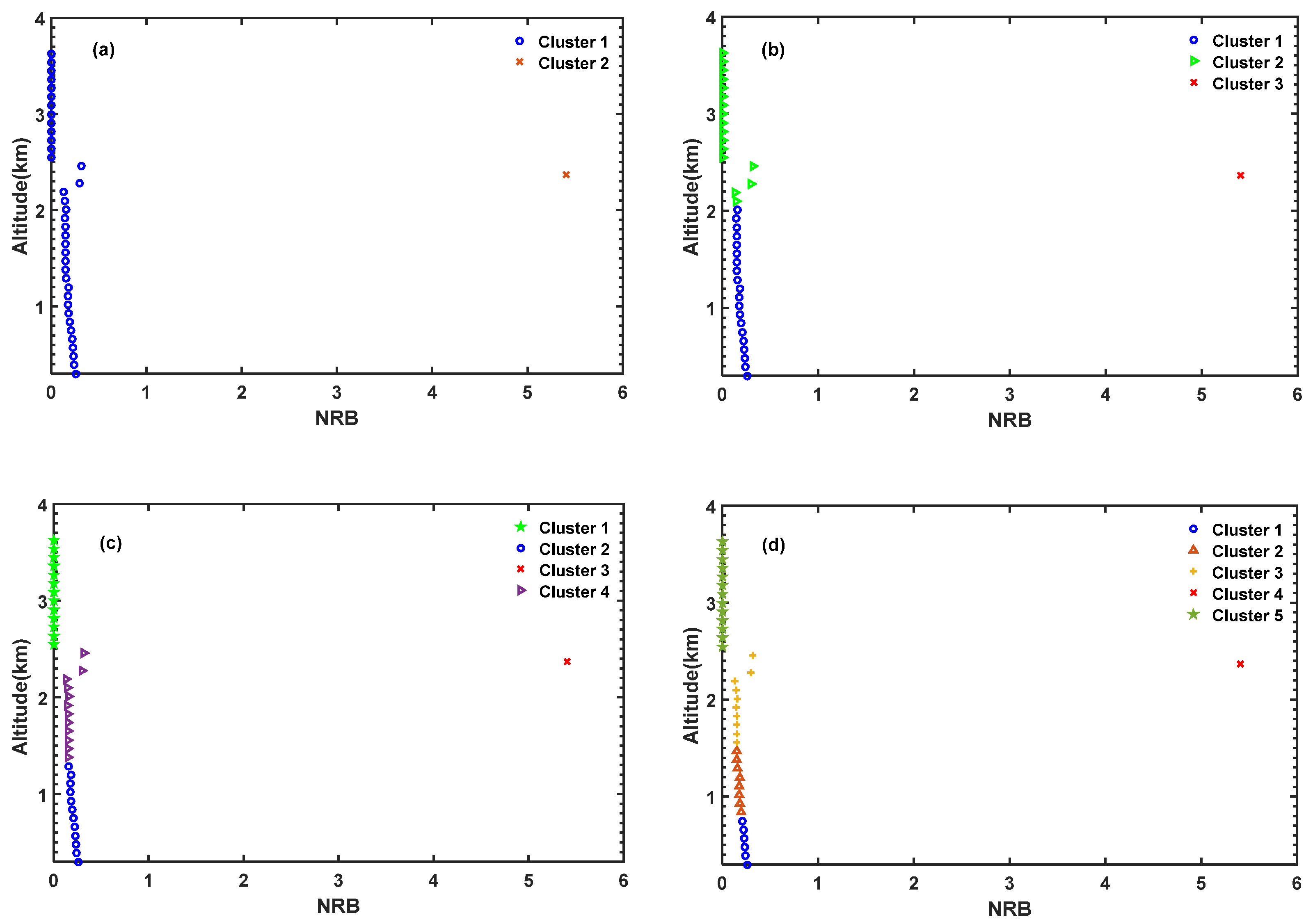
3.3. K-Means Method
3.4. MKnm Method
3.4.1. Algorithm Description
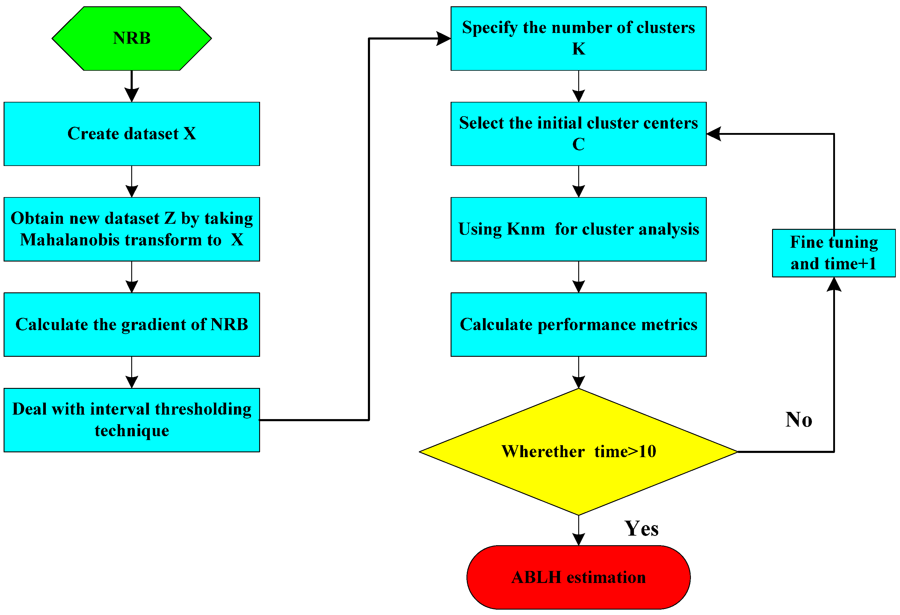
3.4.2. Flowchart of ABLH Estimated by MKnm
3.4.3. Performance Metrics
4. Results
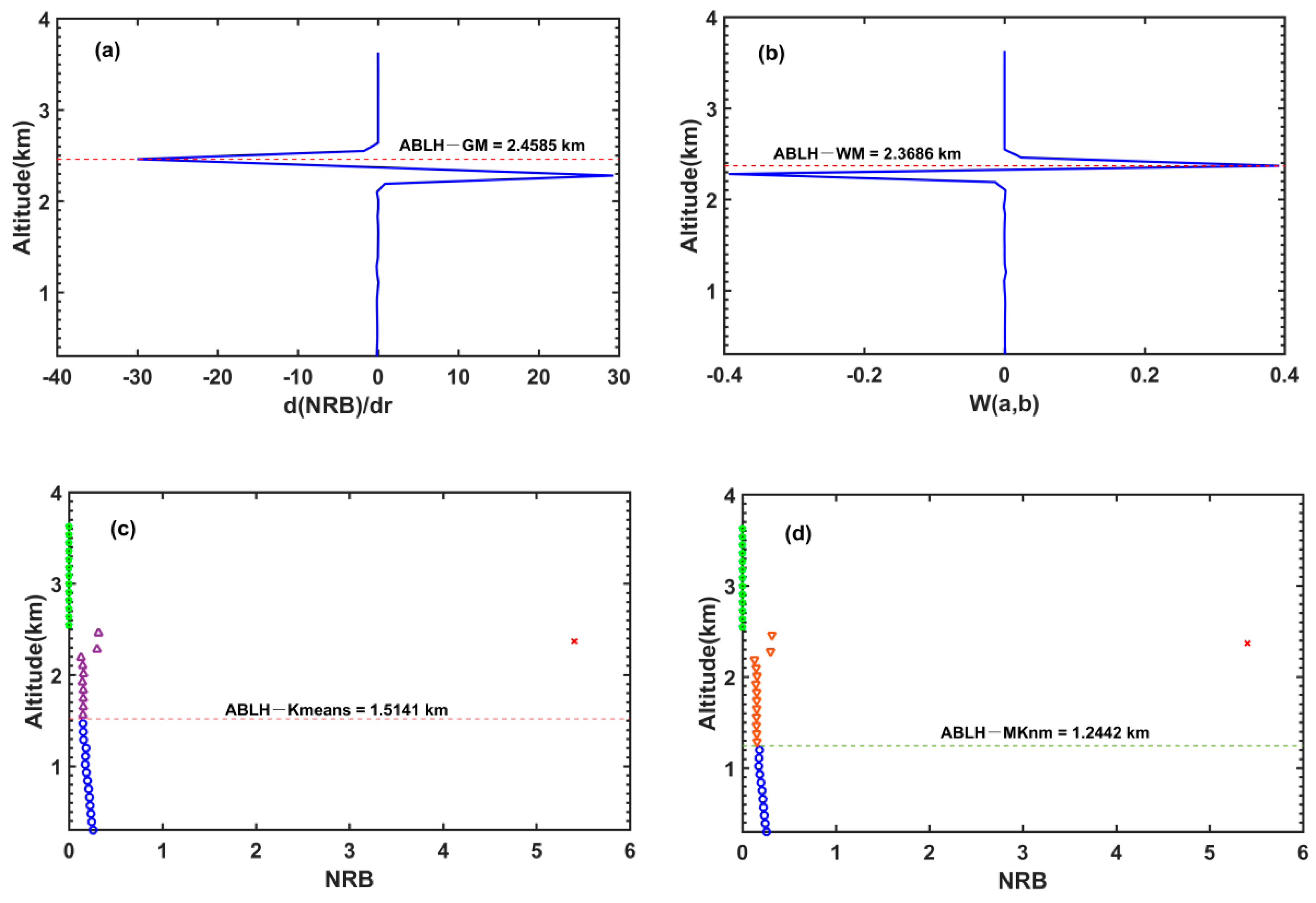
4.1. ABLH Estimated by Different Methods
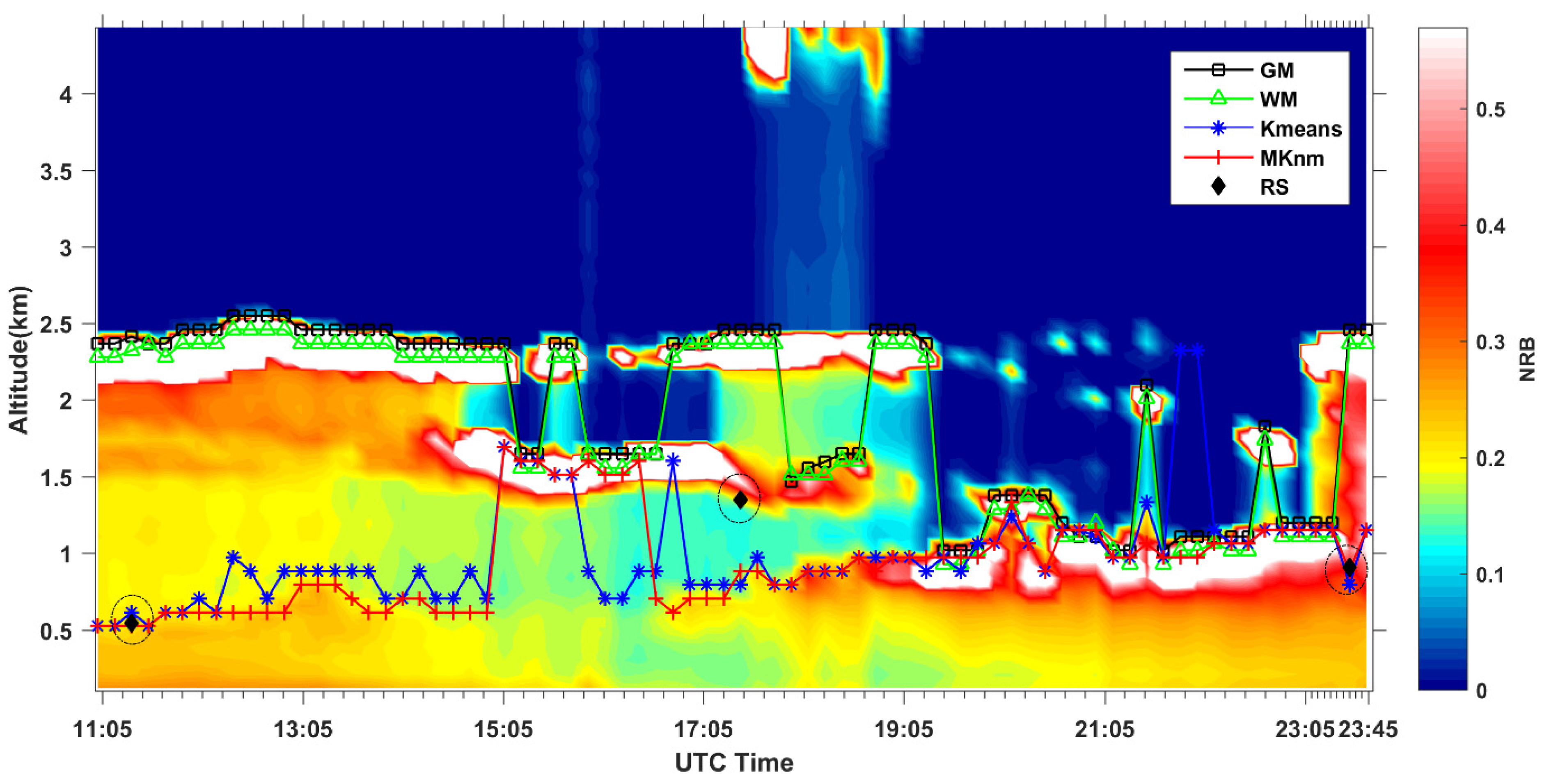
4.2. ABLH Diurnal Cycles under Cloudy Conditions
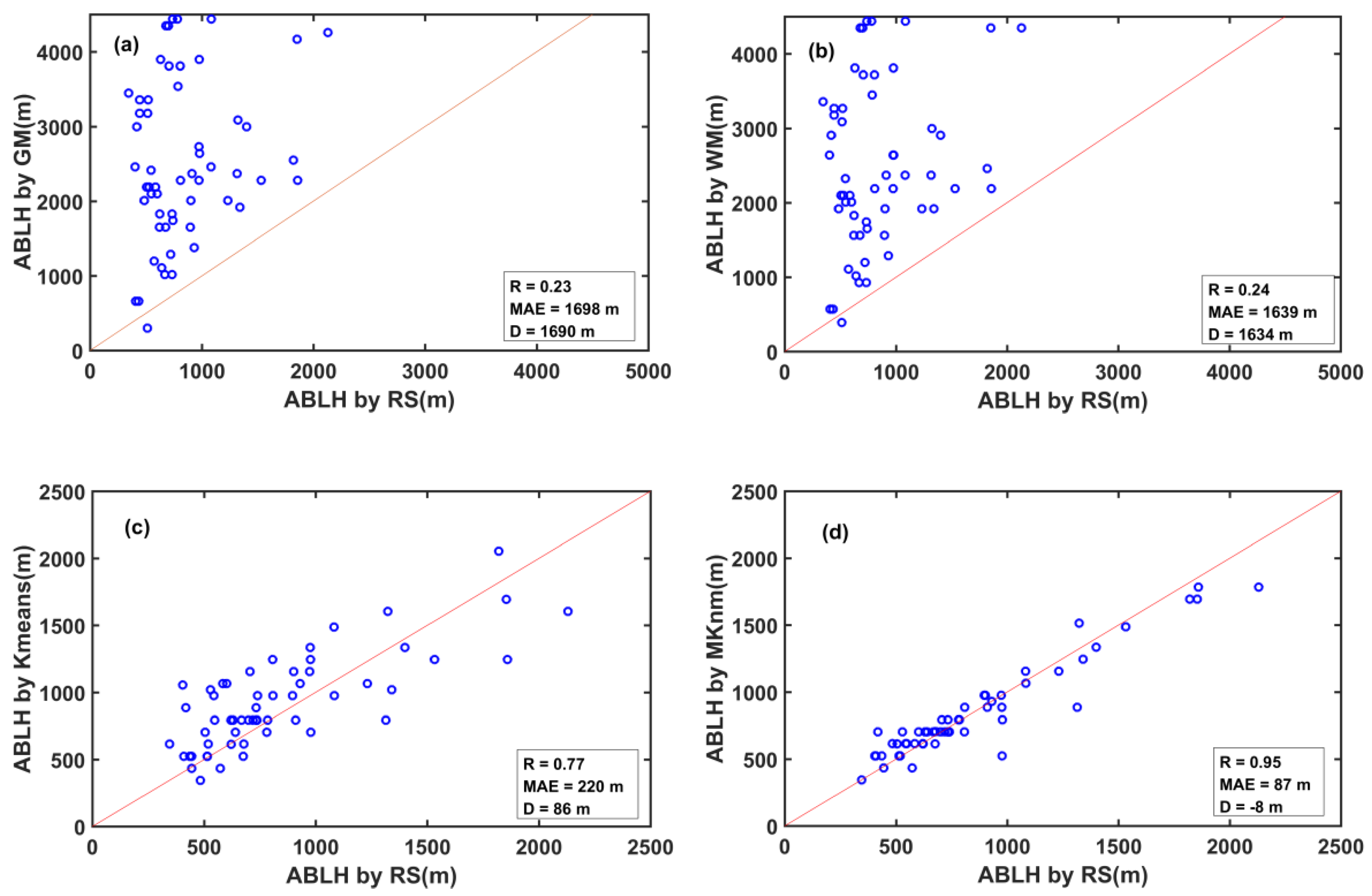
4.3. Comparisons of ABLH Retrieval between LiDAR and Radiosonde Methods under Clouds or RL Conditions
5. Discussion
5.1. Evaluation Index to Quantify the Quality of Clustering
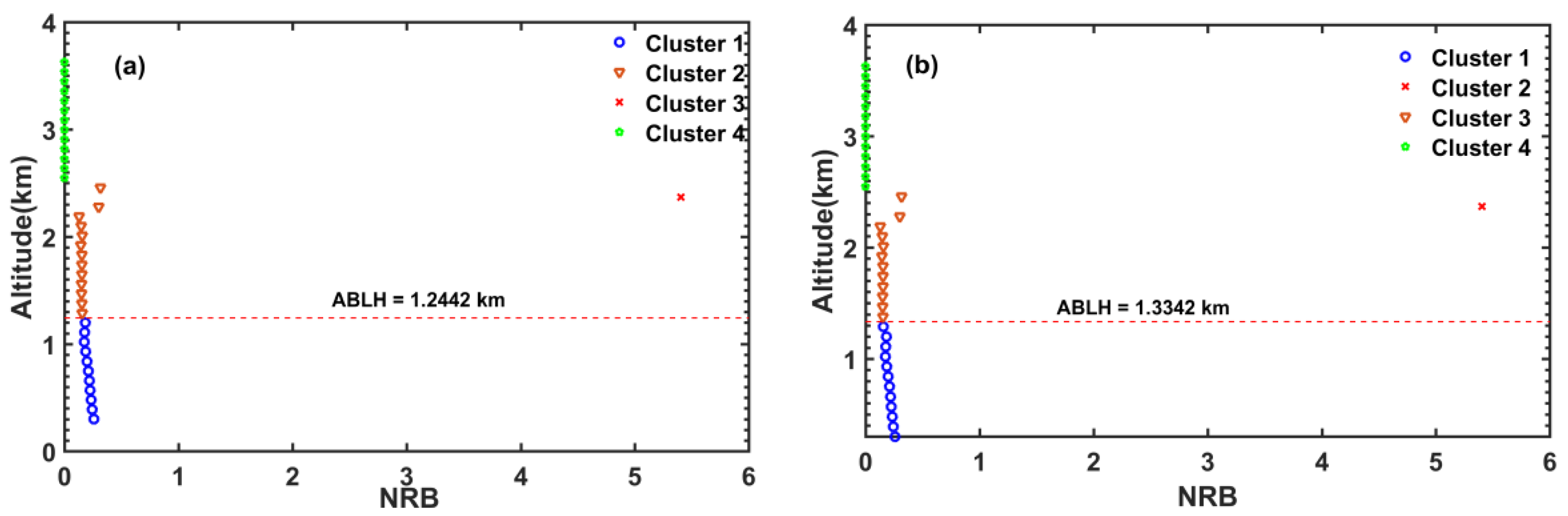
5.2. Define the ABLH after Clustering
5.3. Estimation of ABLH above the Cloud
6. Conclusions
Author Contributions
Funding
Data Availability Statement
Acknowledgments
Conflicts of Interest
Abbreviations
| Atmospheric boundary layer | ABL |
| Atmospheric boundary layer height | ABLH |
| Radiosonde | RS |
| Free Troposphere | FT |
| Entrainment zone | EZ |
| Gradient method | GM |
| Wavelet covariance transform method | WM |
| Machine learning | ML |
| Cluster analysis | CA |
| Residual layer | RL |
| Mahalanobis transform K-near-means | MKnm |
| Micro-pulse LiDAR | MPL |
| Southern Great Plains | SGP |
| Atmospheric Radiation Measurement | ARM |
| Normalized relative backscatter | NRB |
| Value-added data product | VAP |
| Sum of the squared errors | SSE |
| Mean of the silhouette coefficient | MSC |
| Davies–Bouldin indices | DBI |
| Mean absolute error | MAE |
References
- Helbig, M.; Gerken, T.; Beamesderfer, E.R.; Baldocchi, D.D.; Banerjee, T.; Biraud, S.C.; Brown, W.O.J.; Brunsell, N.A.; Burakowski, E.A.; Burns, S.P.; et al. Integrating continuous atmospheric boundary layer and tower-based flux measurements to advance understanding of land-atmosphere interactions. Agric. For. Meteorol. 2021, 307, 108509. [Google Scholar] [CrossRef]
- Su, T.; Li, J.; Li, C.; Xiang, P.; Lau, A.K.H.; Guo, J.; Yang, D.; Miao, Y. An intercomparison of long-term planetary boundary layer heights retrieved from CALIPSO, ground-based lidar, and radiosonde measurements over Hong Kong. J. Geophys. Res. 2017, 122, 3929–3943. [Google Scholar] [CrossRef]
- Kim, M.H.; Yeo, H.; Park, S.; Park, D.H.; Omar, A.; Nishizawa, T.; Shimizu, A.; Kim, S.W. Assessing CALIOP-derived planetary boundary layer height using ground-based lidar. Remote Sens. 2021, 13, 1496. [Google Scholar] [CrossRef]
- Feudo, T.L.; Calidonna, C.R.; Avolio, E.; Sempreviva, A.M. Study of the Vertical Structure of the Coastal Boundary Layer Integrating Surface Measurements and Ground-Based Remote Sensing. Sensors 2020, 13, 6516. [Google Scholar] [CrossRef]
- Zhang, Y.; Chen, S.; Chen, S.; Chen, H.; Guo, P. A novel lidar gradient cluster analysis method of nocturnal boundary layer detection during air pollution episodes. Atmos. Meas. Tech. 2020, 13, 6675–6689. [Google Scholar] [CrossRef]
- Wang, D.; Szczepanik, D.; Stachlewska, I.S. Interrelations between surface, boundary layer, and columnar aerosol properties derived in summer and early autumn over a continental urban site in Warsaw, Poland. Atmos. Chem. Phys. 2019, 19, 13097–13128. [Google Scholar] [CrossRef] [Green Version]
- Fang, Z.; Yang, H.; Cao, Y.; Xing, K.; Liu, D.; Zhao, M.; Xie, C. Study of persistent pollution in hefei during winter revealed by ground-based LiDAR and the CALIPSO satellite. Sustainability 2021, 13, 875. [Google Scholar] [CrossRef]
- Bain, C.L.; Parker, D.J.; Taylor, C.M.; Kergoat, L.; Guichard, F. Observations of the nocturnal boundary layer associated with the West African monsoon. Mon. Weather Rev. 2010, 138, 3142–3156. [Google Scholar] [CrossRef] [Green Version]
- Moreira, G.d.A.; Guerrero-Rascado, J.L.; Bravo-Aranda, J.A.; Foyo-Moreno, I.; Cazorla, A.; Alados, I.; Lyamani, H.; Landulfo, E.; Alados-Arboledas, L. Study of the planetary boundary layer height in an urban environment using a combination of microwave radiometer and ceilometer. Atmos. Res. 2020, 240, 104932. [Google Scholar] [CrossRef]
- Liu, S.; Liang, X.Z. Observed diurnal cycle climatology of planetary boundary layer height. J. Clim. 2010, 23, 5790–5809. [Google Scholar] [CrossRef]
- Guo, J.; Li, Y.; Cohen, J.B.; Li, J.; Chen, D.; Xu, H.; Liu, L.; Yin, J.; Hu, K.; Zhai, P. Shift in the Temporal Trend of Boundary Layer Height in China Using Long-Term (1979–2016) Radiosonde Data. Geophys. Res. Lett. 2019, 46, 6080–6089. [Google Scholar] [CrossRef] [Green Version]
- Seidel, D.J.; Ao, C.O.; Li, K. Estimating climatological planetary boundary layer heights from radiosonde observations: Comparison of methods and uncertainty analysis. J. Geophys. Res. Atmos. 2010, 115, 16113. [Google Scholar] [CrossRef] [Green Version]
- Korhonen, K.; Giannakaki, E.; Mielonen, T.; Pfüller, A.; Laakso, L.; Vakkari, V.; Baars, H.; Engelmann, R.; Beukes, J.P.; Van Zyl, P.G.; et al. Atmospheric boundary layer top height in South Africa: Measurements with lidar and radiosonde compared to three atmospheric models. Atmos. Chem. Phys. 2014, 14, 4263–4278. [Google Scholar] [CrossRef] [Green Version]
- Li, H.; Chang, J.; Liu, Z.; Zhang, L.; Dai, T.; Chen, S. An improved method for automatic determination of the planetary boundary layer height based on lidar data. J. Quant. Spectrosc. Radiat. Transf. 2020, 257, 107382. [Google Scholar] [CrossRef]
- Du, L.; Pan, Y.; Wang, W. Random sample fitting method to determine the planetary boundary layer height using satellite-based lidar backscatter profiles. Remote Sens. 2020, 12, 4006. [Google Scholar] [CrossRef]
- Dang, R.; Yang, Y.; Hu, X.M.; Wang, Z.; Zhang, S. A review of techniques for diagnosing the atmospheric boundary layer height (ABLH) using aerosol lidar data. Remote Sens. 2019, 11, 1590. [Google Scholar] [CrossRef] [Green Version]
- Caicedo, V.; Rappenglück, B.; Lefer, B.; Morris, G.; Toledo, D.; Delgado, R. Comparison of aerosol lidar retrieval methods for boundary layer height detection using ceilometer aerosol backscatter data. Atmos. Meas. Tech. 2017, 10, 1609–1622. [Google Scholar] [CrossRef] [Green Version]
- Toledo, D.; Córdoba-Jabonero, C.; Adame, J.A.; De La Morena, B.; Gil-Ojeda, M. Estimation of the atmospheric boundary layer height during different atmospheric conditions: A comparison on reliability of several methods applied to lidar measurements. Int. J. Remote Sens. 2017, 38, 3203–3218. [Google Scholar] [CrossRef]
- Melfi, S.H.; Spinhirne, J.D.; Chou, S.H.; Palm, S.P. Lidar observations of vertically organized convection in the planetary boundary layer over the ocean. J. Clim. Appl. Meteorol. 1985, 24, 806–821. [Google Scholar] [CrossRef]
- Hayden, K.L.; Anlauf, K.G.; Hoff, R.M.; Strapp, J.W.; Bottenheim, J.W.; Wiebe, H.A.; Froude, F.A.; Martin, J.B.; Steyn, D.G.; McKendry, I.G. The vertical chemical and meteorological structure of the boundary layer in the Lower Fraser Valley during Pacific ’93. Atmos. Environ. 1997, 31, 2089–2105. [Google Scholar] [CrossRef]
- Compton, J.C.; Delgado, R.; Berkoff, T.A.; Hoff, R.M. Determination of planetary boundary layer height on short spatial and temporal scales: A demonstration of the covariance wavelet transform in ground-based wind profiler and lidar measurements. J. Atmos. Ocean. Technol. 2013, 30, 1566–1575. [Google Scholar] [CrossRef]
- Menut, L.; Flamant, C.; Pelon, J.; Flamant, P.H. Urban boundary-layer height determination from lidar measurements over the Paris area. Appl. Opt. 1999, 38, 945. [Google Scholar] [CrossRef]
- Kang, J.; Ullah, Z.; Gwak, J. Mri-based brain tumor classification using ensemble of deep features and machine learning classifiers. Sensors 2021, 21, 2222. [Google Scholar] [CrossRef]
- Al-Sahaf, H.; Bi, Y.; Chen, Q.; Lensen, A.; Mei, Y.; Sun, Y.; Tran, B.; Xue, B.; Zhang, M. A survey on evolutionary machine learning. J. R. Soc. N. Z. 2019, 49, 205–228. [Google Scholar] [CrossRef]
- Li, Y.; Yu, F.; Cai, Q.; Qian, M.; Liu, P.; Guo, J.; Yan, H.; Yuan, K.; Yu, J. Design of Target Recognition System Based on Machine Learning Hardware Accelerator. Wirel. Pers. Commun. 2018, 102, 1557–1571. [Google Scholar] [CrossRef]
- Zhang, F.; Li, W.; Zhang, Y.; Feng, Z. Data Driven Feature Selection for Machine Learning Algorithms in Computer Vision. IEEE Internet Things J. 2018, 5, 4262–4272. [Google Scholar] [CrossRef]
- Maxwell, A.E.; Warner, T.A.; Fang, F. Implementation of machine-learning classification in remote sensing: An applied review. Int. J. Remote Sens. 2018, 39, 2784–2817. [Google Scholar] [CrossRef] [Green Version]
- Yu, W.; Liu, Y.; Ma, Z.; Bi, J. Improving satellite-based PM2.5 estimates in China using Gaussian processes modeling in a Bayesian hierarchical setting. Sci. Rep. 2017, 7, 7048. [Google Scholar] [CrossRef] [Green Version]
- Liu, Z.; Chang, J.; Li, H.; Zhang, L.; Chen, S. Signal Denoising Method Combined with Variational Mode Decomposition, Machine Learning Online Optimization and the Interval Thresholding Technique. IEEE Access 2020, 8, 223482–223494. [Google Scholar] [CrossRef]
- Toledo, D.; Córdoba-Jabonero, C.; Gil-Ojeda, M. Cluster analysis: A new approach applied to lidar measurements for atmospheric boundary layer height estimation. J. Atmos. Ocean. Technol. 2014, 31, 422–436. [Google Scholar] [CrossRef]
- Rieutord, T.; Aubert, S.; MacHado, T. Deriving boundary layer height from aerosol lidar using machine learning: KABL and ADABL algorithms. Atmos. Meas. Tech. 2021, 14, 4335–4353. [Google Scholar] [CrossRef]
- Rossow, W.B.; Schiffer, R.A. Advances in Understanding Clouds from ISCCP. Bull. Am. Meteorol. Soc. 1999, 80, 2261–2287. [Google Scholar] [CrossRef] [Green Version]
- Krishnamurthy, R.; Newsom, R.K.; Berg, L.K.; Xiao, H.; Ma, P.L.; Turner, D.D. On the estimation of boundary layer heights: A machine learning approach. Atmos. Meas. Tech. 2021, 14, 4403–4424. [Google Scholar] [CrossRef]
- Dang, R.; Yang, Y.; Li, H.; Hu, X.M.; Wang, Z.; Huang, Z.; Zhou, T.; Zhang, T. Atmosphere boundary layer height (ABLH) determination under multiple-layer conditions using micro-pulse lidar. Remote Sens. 2019, 11, 263. [Google Scholar] [CrossRef] [Green Version]
- Zhong, T.; Wang, N.; Shen, X.; Xiao, D.; Xiang, Z.; Liu, D. Determination of planetary boundary layer height with lidar signals using maximum limited height initialization and range restriction (MLHI-RR). Remote Sens. 2020, 12, 2272. [Google Scholar] [CrossRef]
- Campbell, J.R.; Hlavka, D.L.; Welton, E.J.; Flynn, C.J.; Turner, D.D.; Spinhirne, J.D.; Stanley, S.; Hwang, I.H. Full-time, eye-safe cloud and aerosol lidar observation at atmospheric radiation measurement program sites: Instruments and data processing. J. Atmos. Ocean. Technol. 2002, 19, 431–442. [Google Scholar] [CrossRef]
- Welton, E.J.; Campbell, J.R.; Spinhirne, J.D.; Scott III, V.S. Global monitoring of clouds and aerosols using a network of micropulse lidar systems. Lidar Remote Sens. Ind. Environ. Monit. 2001, 4153, 151. [Google Scholar] [CrossRef]
- Li, H.; Liu, B.; Ma, X.; Jin, S.; Ma, Y.; Zhao, Y.; Gong, W. Evaluation of retrieval methods for planetary boundary layer height based on radiosonde data. Atmos. Meas. Tech. 2021, 14, 5977–5986. [Google Scholar] [CrossRef]
- Min, J.S.; Park, M.S.; Chae, J.H.; Kang, M. Integrated System for Atmospheric Boundary Layer Height Estimation (ISABLE) using a ceilometer and microwave radiometer. Atmos. Meas. Tech. 2020, 13, 6965–6987. [Google Scholar] [CrossRef]
- Qi, J.; Yu, Y.; Wang, L.; Liu, J.; Wang, Y. An effective and efficient hierarchical K-means clustering algorithm. Int. J. Distrib. Sens. Netw. 2017, 13, 8. [Google Scholar] [CrossRef] [Green Version]
- Xiang, S.; Nie, F.; Zhang, C. Learning a Mahalanobis distance metric for data clustering and classification. Pattern Recognit. 2008, 41, 3600–3612. [Google Scholar] [CrossRef]
- Omara, I.; Hagag, A.; Ma, G.; El-Samie, F.E.A.; Song, E. A novel approach for ear recognition: Learning Mahalanobis distance features from deep CNNs. Mach. Vis. Appl. 2021, 32, 38. [Google Scholar] [CrossRef]
- Lovmar, L.; Ahlford, A.; Jonsson, M.; Syvänen, A.C. Silhouette scores for assessment of SNP genotype clusters. BMC Genom. 2005, 6, 35. [Google Scholar] [CrossRef]
- Davies, D.L.; Bouldin, D.W. A Cluster Separation Measure. IEEE Trans. Pattern Anal. Mach. Intell. 1979, PAMI-1, 224–227. [Google Scholar] [CrossRef]
- Pal, S.R.; Steinbrecht, W.; Carswell, A.I. Automated method for lidar determination of cloud-base height and vertical extent. Appl. Opt. 1992, 31, 1488. [Google Scholar] [CrossRef] [PubMed]


| Method | R | MAE(m) | D(m) |
|---|---|---|---|
| GM | 0.23 | 1698 | 1690 |
| WM | 0.24 | 1639 | 1634 |
| K-means | 0.77 | 220 | 86 |
| MKnm | 0.95 | 87 | −8 |
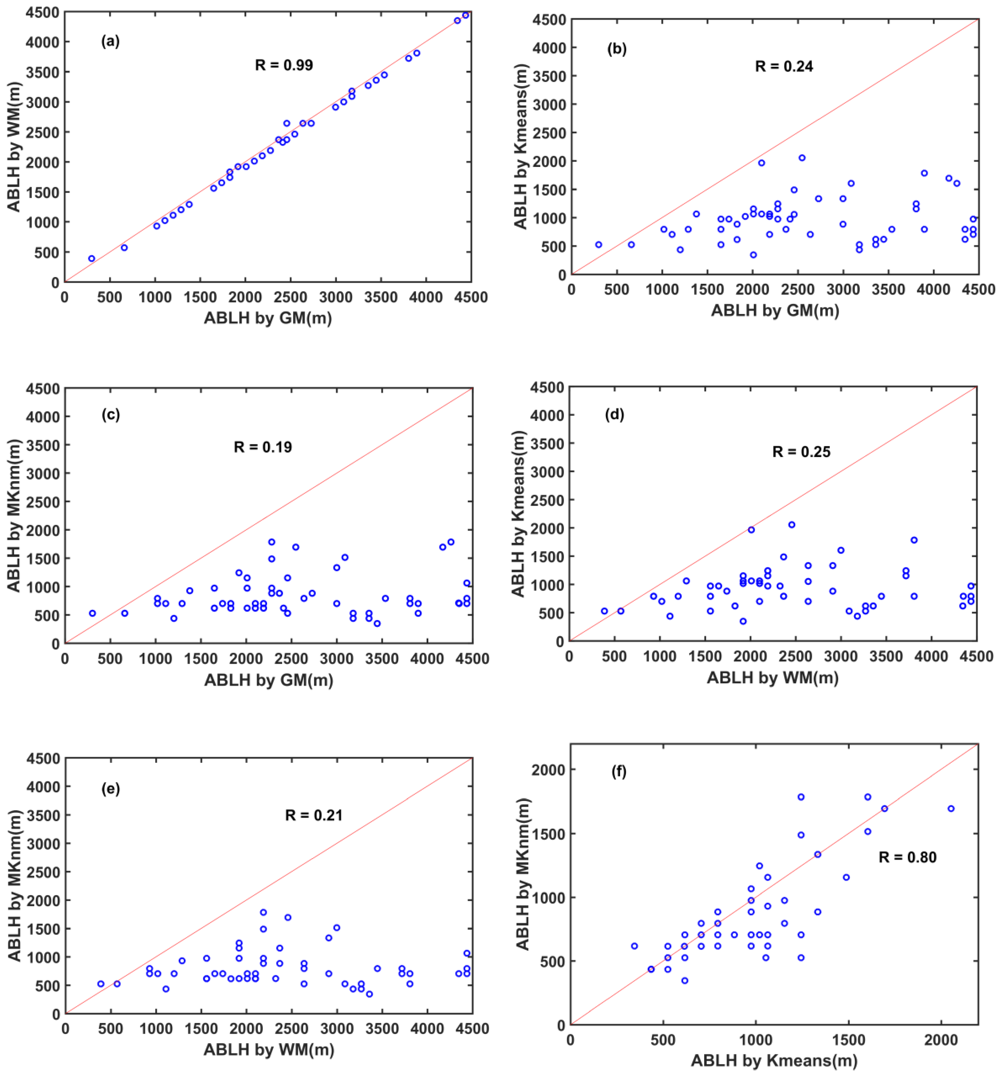
| GM | WM | K-means | MKnm | |
|---|---|---|---|---|
| GM | 1 | 0.99 | 0.24 | 0.19 |
| WM | 0.99 | 1 | 0.25 | 0.21 |
| K-means | 0.24 | 0.25 | 1 | 0.80 |
| MKnm | 0.19 | 0.21 | 0.80 | 1 |
Publisher’s Note: MDPI stays neutral with regard to jurisdictional claims in published maps and institutional affiliations. |
© 2022 by the authors. Licensee MDPI, Basel, Switzerland. This article is an open access article distributed under the terms and conditions of the Creative Commons Attribution (CC BY) license (https://creativecommons.org/licenses/by/4.0/).
Share and Cite
Liu, Z.; Chang, J.; Li, H.; Chen, S.; Dai, T. Estimating Boundary Layer Height from LiDAR Data under Complex Atmospheric Conditions Using Machine Learning. Remote Sens. 2022, 14, 418. https://doi.org/10.3390/rs14020418
Liu Z, Chang J, Li H, Chen S, Dai T. Estimating Boundary Layer Height from LiDAR Data under Complex Atmospheric Conditions Using Machine Learning. Remote Sensing. 2022; 14(2):418. https://doi.org/10.3390/rs14020418
Chicago/Turabian StyleLiu, Zhenxing, Jianhua Chang, Hongxu Li, Sicheng Chen, and Tengfei Dai. 2022. "Estimating Boundary Layer Height from LiDAR Data under Complex Atmospheric Conditions Using Machine Learning" Remote Sensing 14, no. 2: 418. https://doi.org/10.3390/rs14020418