
3D Modeling of Urban Area Based on Oblique UAS Images—An End-to-End Pipeline


Abstract
:1. Introduction
- –
- Type of data used: optical (monoscopy, stereoscopy, multiscopy), LiDAR data: terrestrial (TLS) and airborne (ALS), UAS images, topographic measurements;
- –
- System automation level: automatic, automatic with cadastral data, semi-automatic;
- –
- Complexity of reconstructed urban areas: dense urban areas, peripheral urban areas, areas of activity and collective housing;
- –
- The degree of generality of 3D modeling: prismatic, parametric, structural or polyhedral;
- –
- 3D modeling methodologies: top-down or model-driven methods, bottom-up or data-driven methods and hypothesize-and-verify.
1.1. Level of Detail and CityGML
1.2. Related Work
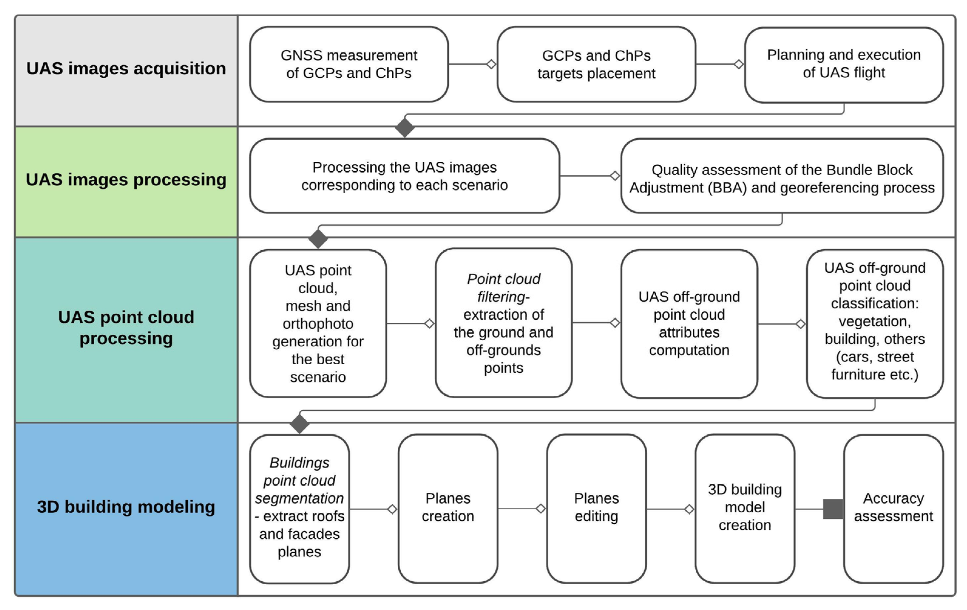
1.3. Proposed Pipeline
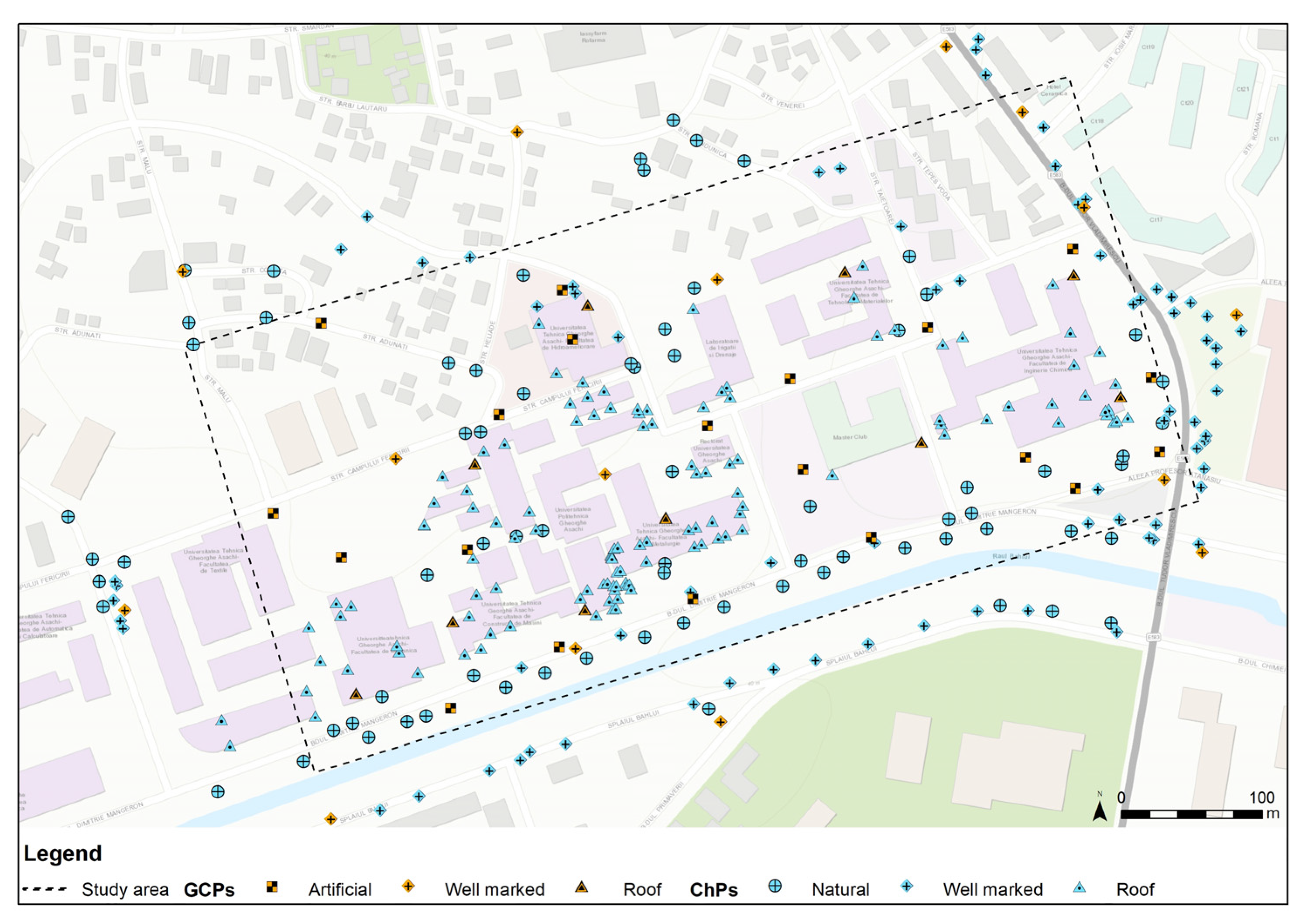
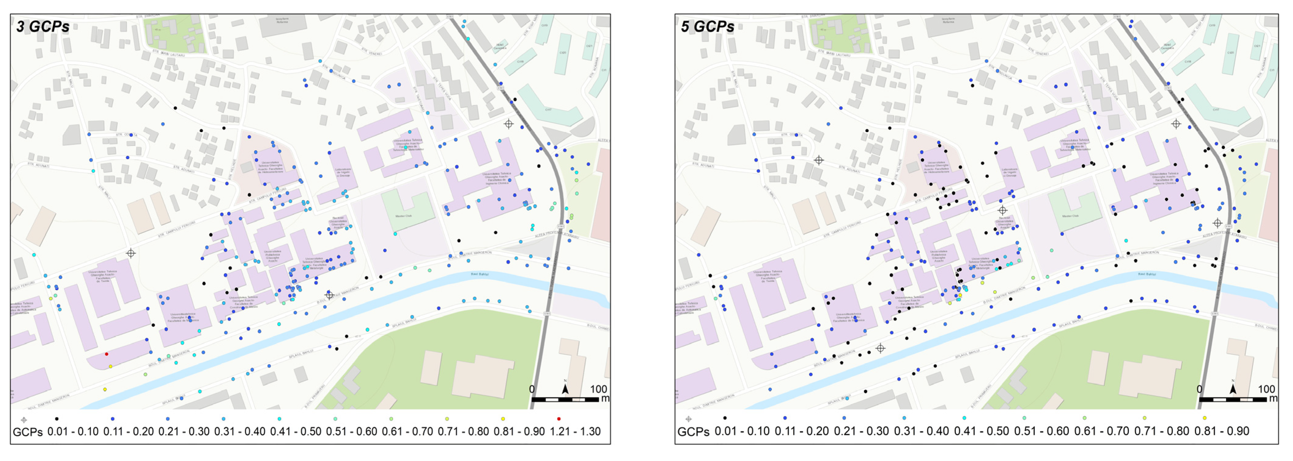
- Using a very high number of Ground Control Points (GCPs) and Check Points (ChPs), i.e., 320, to find the best scenario for UAS images orientation and georeferencing (artificial, well pre-marked by paint and natural points);
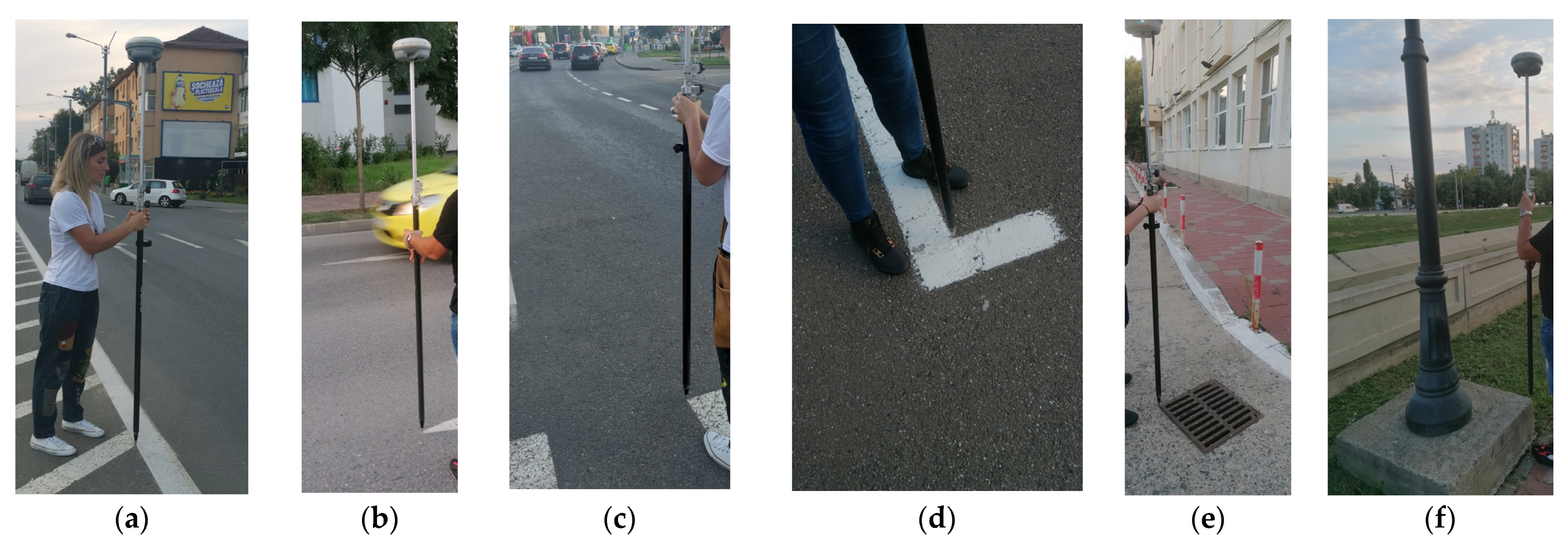
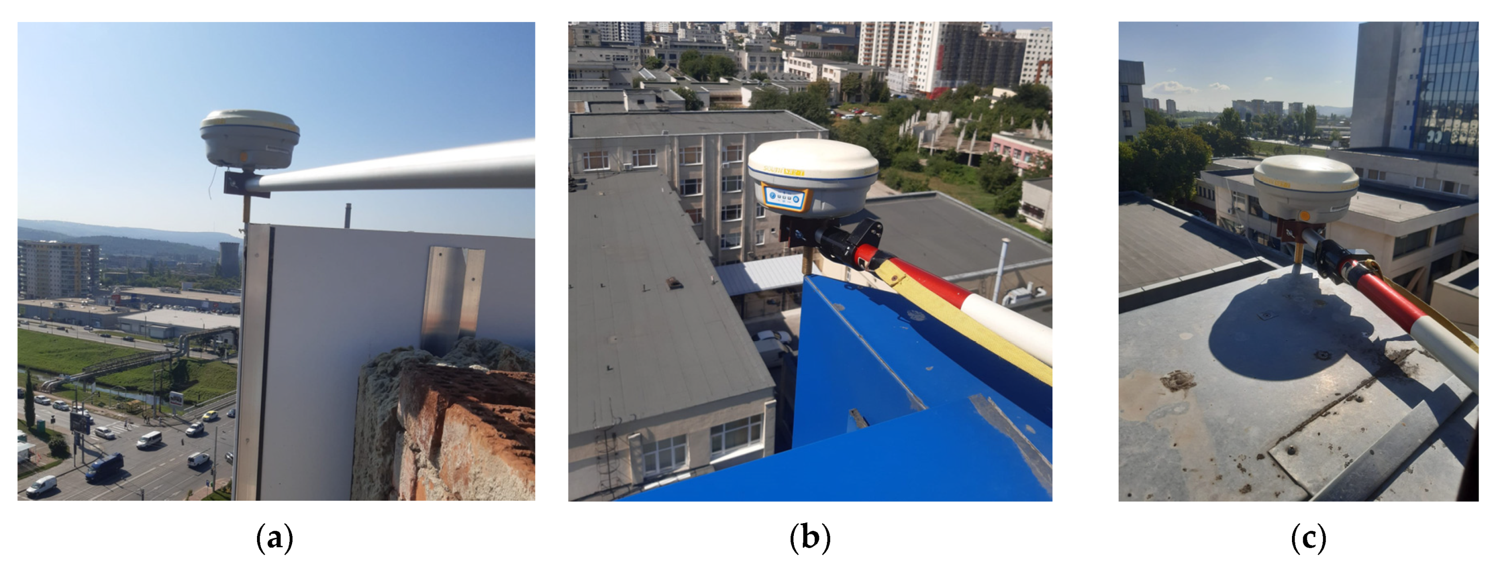
- Taking measurements for buildings’ roof corners using Global Navigation Satellite System-Real Time Kinematic positioning (GNSS-RTK) technology, with the help of a handcrafted dispositive, to test their influence in the BBA process and to assess the 3D buildings models’ accuracy;
- Presenting an end-to-end pipeline for 3D building models generation using only UAS point cloud, from raw data to final 3D models, not taking use of additional information such as buildings’ footprints;
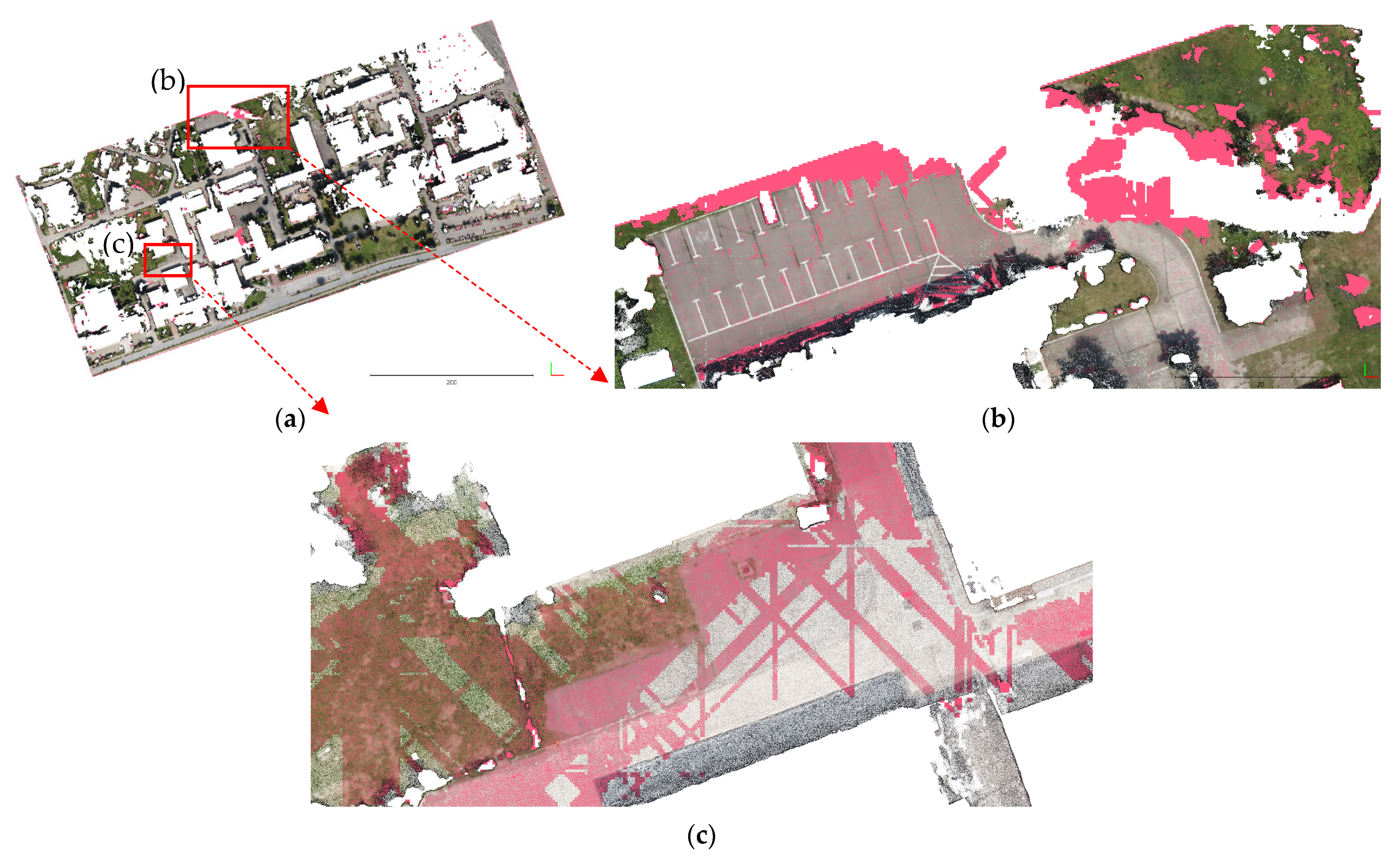
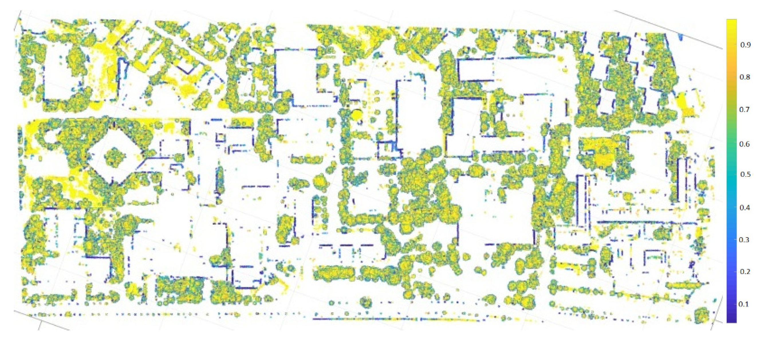
- Presenting a new workflow for automatic extraction of vegetation UAS points, using a combination of point clouds and rasters;
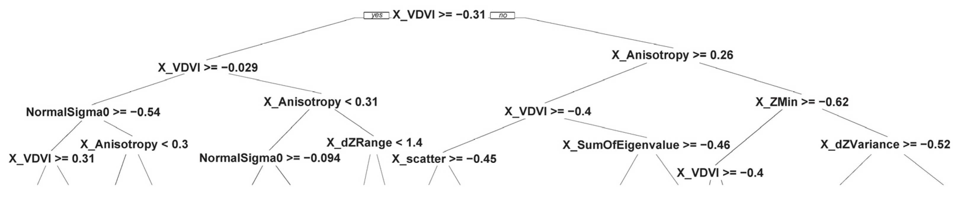
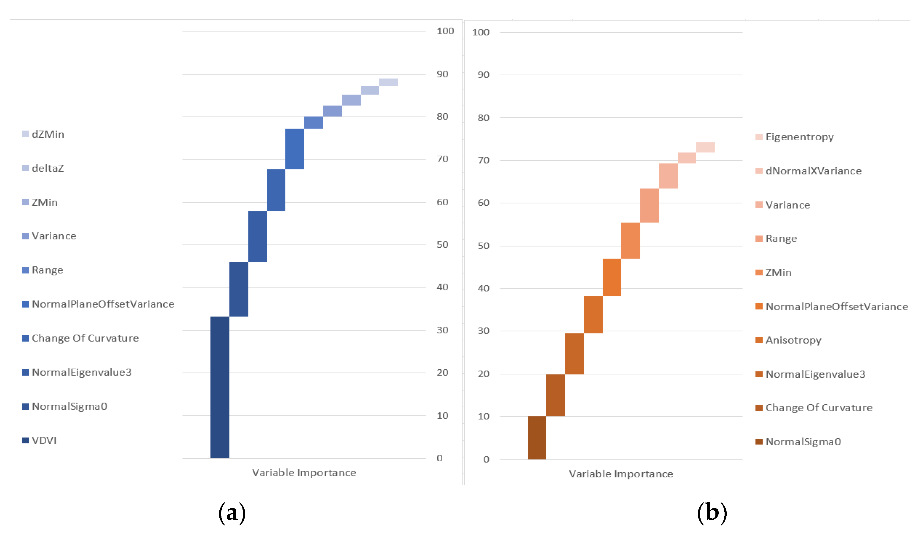
- Finding a key attribute in the process of UAS point cloud classification by random forest algorithm, i.e., the visible-band difference vegetation index (VDVI).
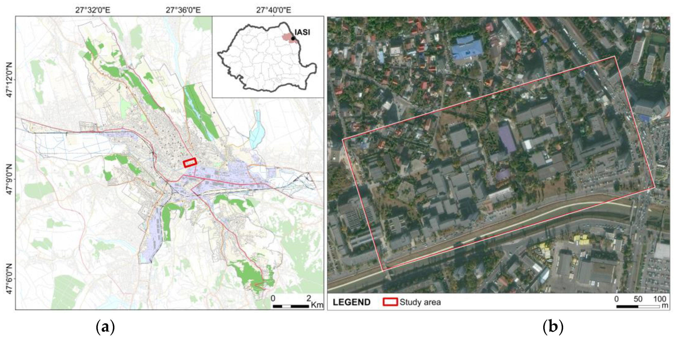
2. Study Area
3. Materials and Methods
3.1. GNSS Measurements
- –
- Position Dilution of Precision (PDOP) 1.15 ÷ 3.99 (<5), mean PDOP = 1.80,
- –
- Horizontal Dilution of Precision (HDOP) 0.63 ÷ 3.16 (<4), mean HDOP = 0.99,
- –
- Vertical Dilution of Precision (VDOP) 0.95 ÷ 3.06 (<4), mean VDOP = 1.49,
- –
- Position Dilution of Precision (PDOP) 1.16 ÷ 3.89 (<5), mean PDOP = 1.73,
- –
- Horizontal Dilution of Precision (HDOP) 0.62 ÷ 2.70 (<4), mean HDOP = 0.93,
- –
- Vertical Dilution of Precision (VDOP) 0.96 ÷ 3.05 (<4), mean VDOP = 1.45,
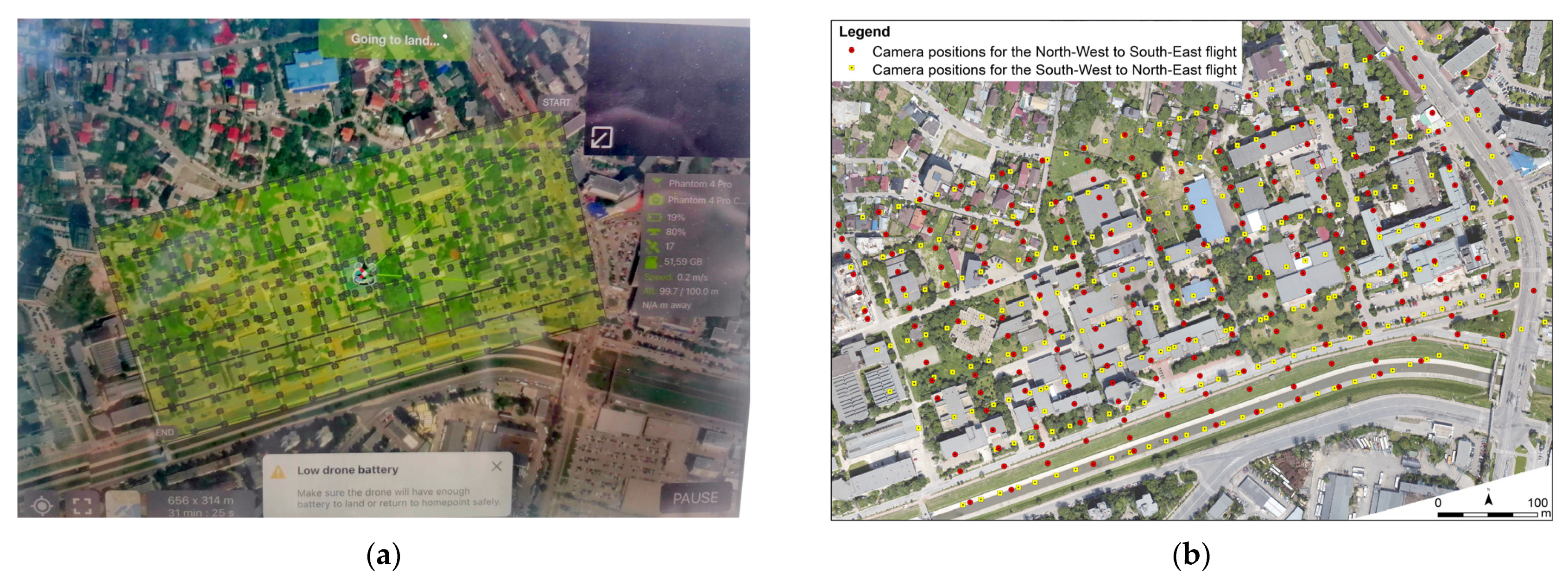
3.2. UAS Images Acquisition
4. Results and Discussions
4.1. UAS Images Processing
- –
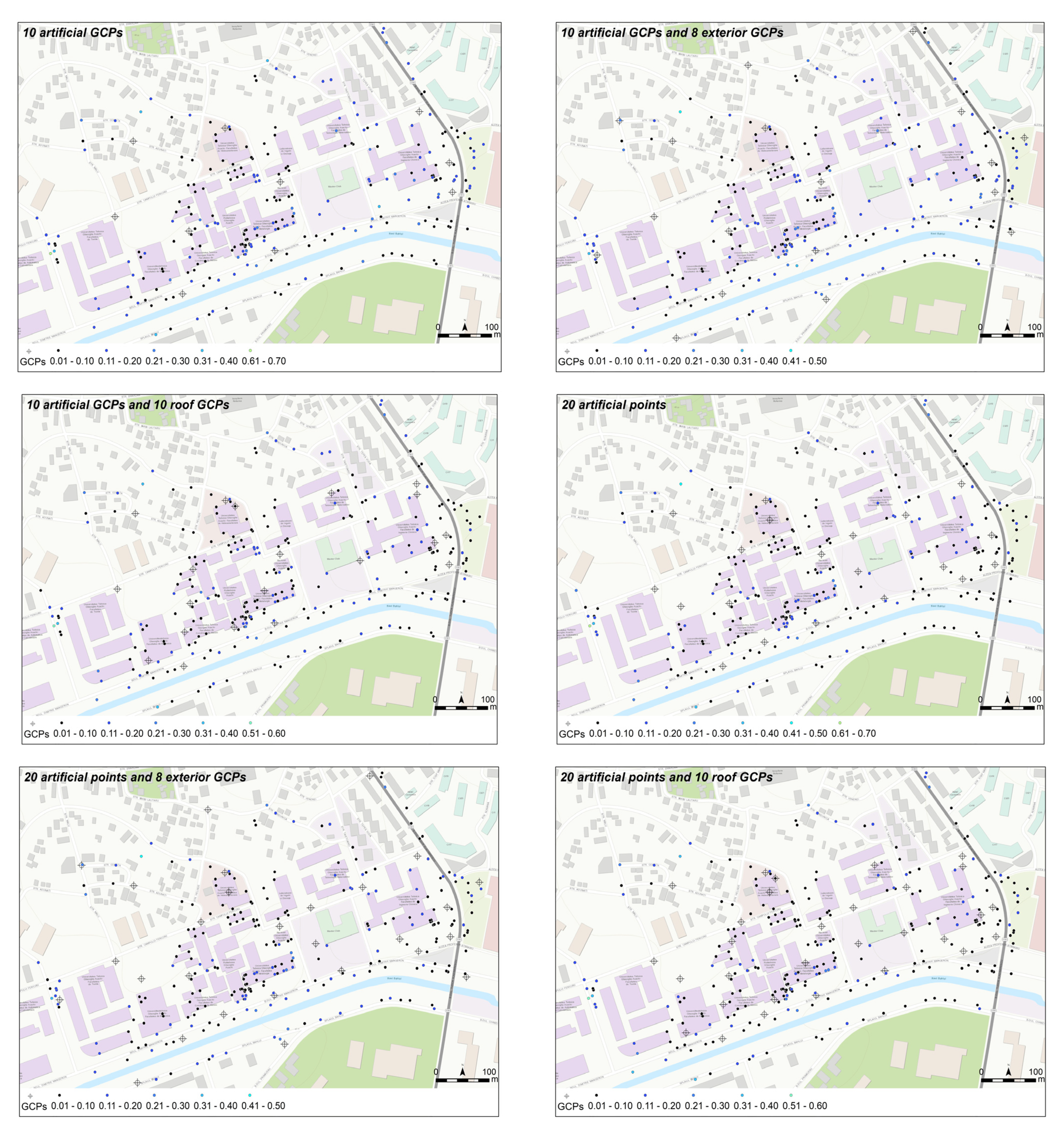
- 20 artificial points uniformly distributed over the study area,
- –
- 10 roof corners uniformly distributed over the study area,
- –
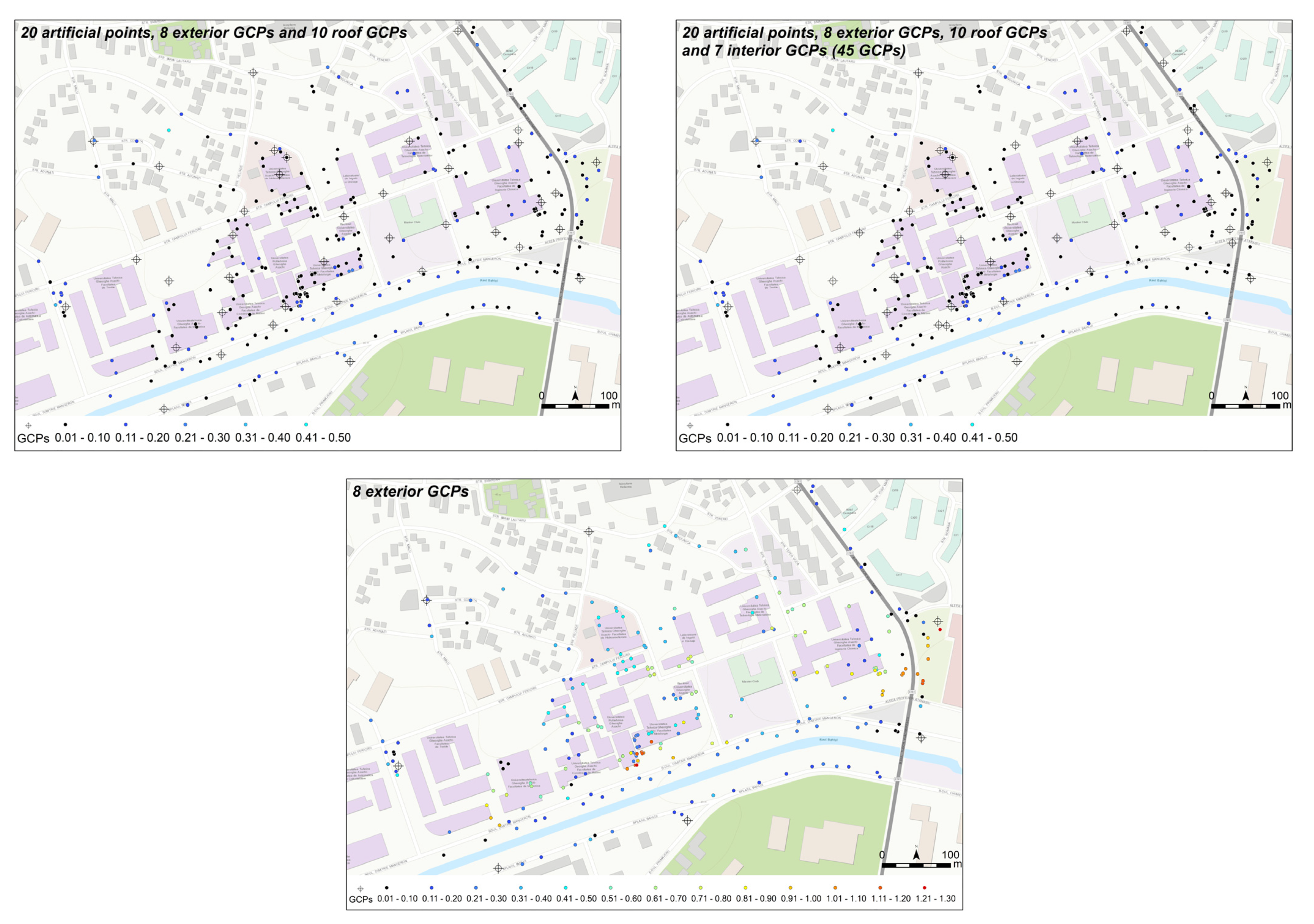
- 8 well marked GCPs situated in the exterior part of the study area,
- –
- 7 natural and well-marked GCPs uniformly distributed over the interior part of the study area.
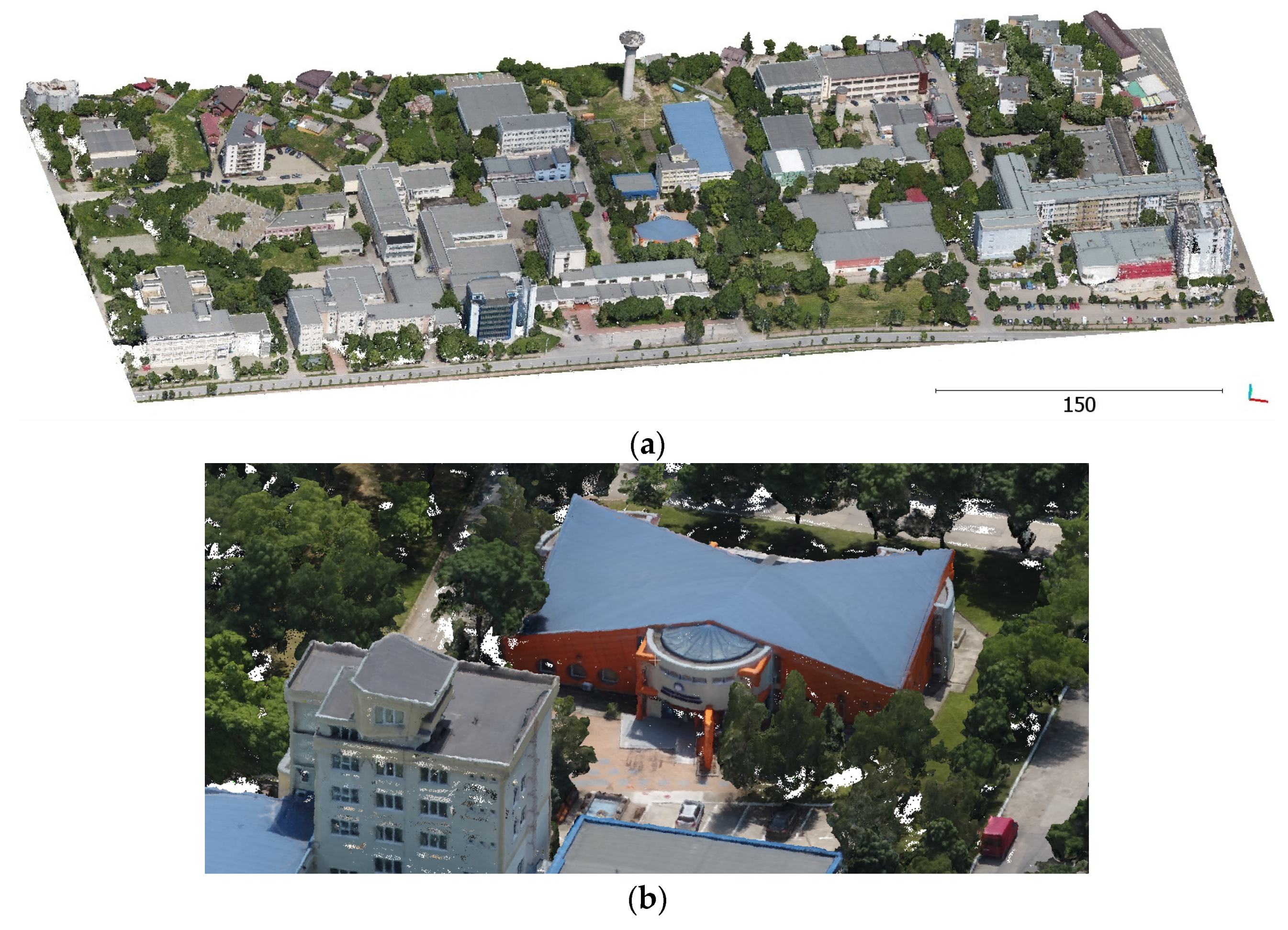
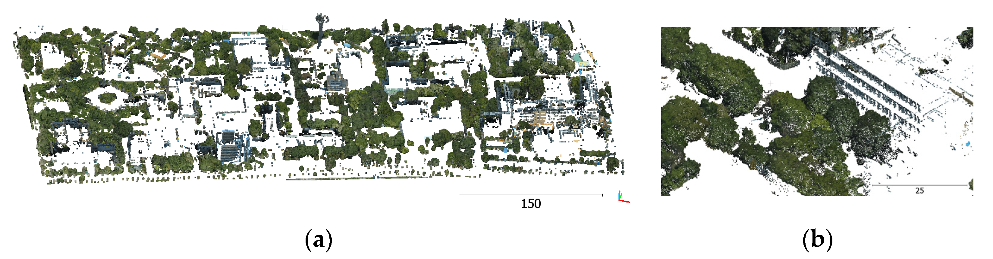
4.2. UAS Point Cloud Generation
4.3. UAS Point Cloud Processing
4.3.1. UAS Point Cloud Classification in Ground and Off-Ground Points
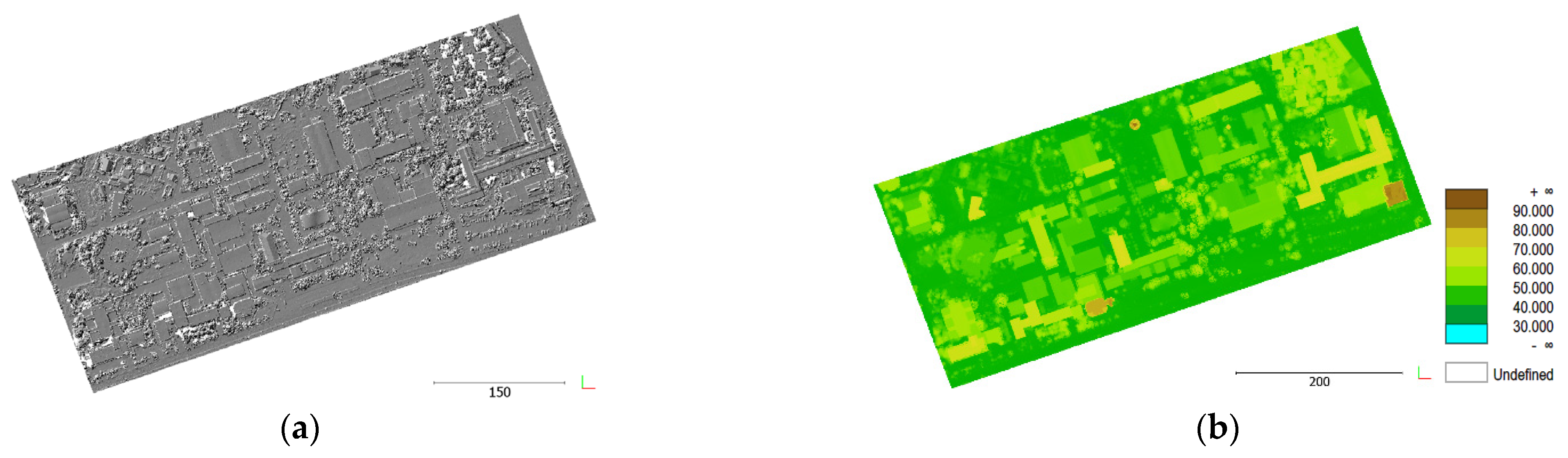
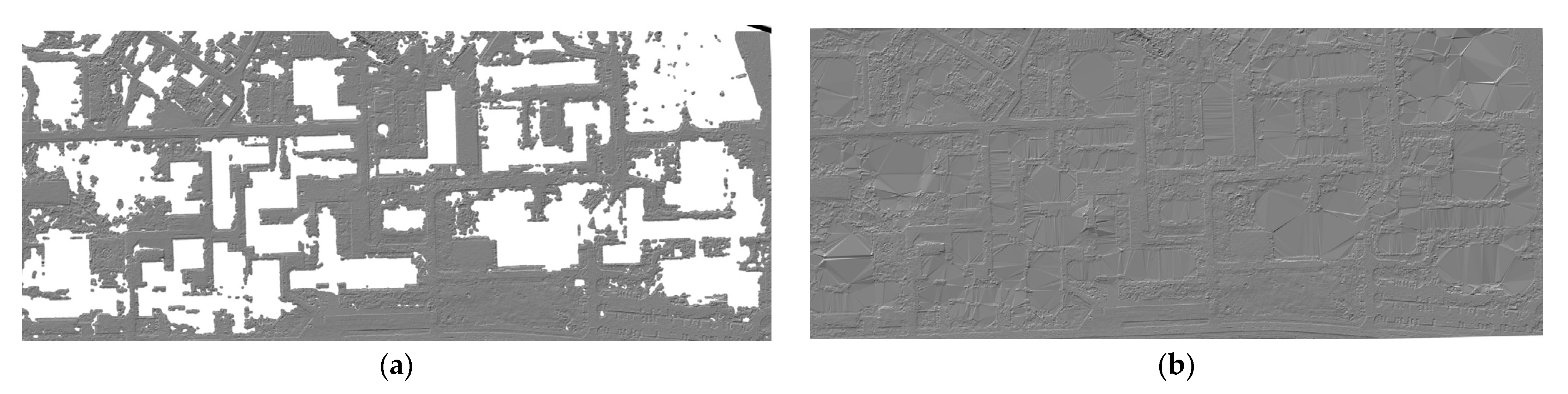
4.3.2. DTM Creation
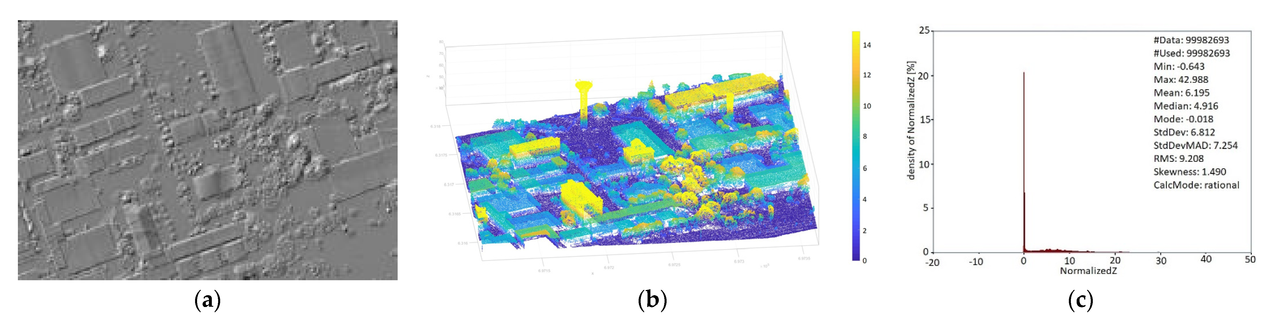
4.3.3. Normalized Digital Surface Model (nDSM) Creation
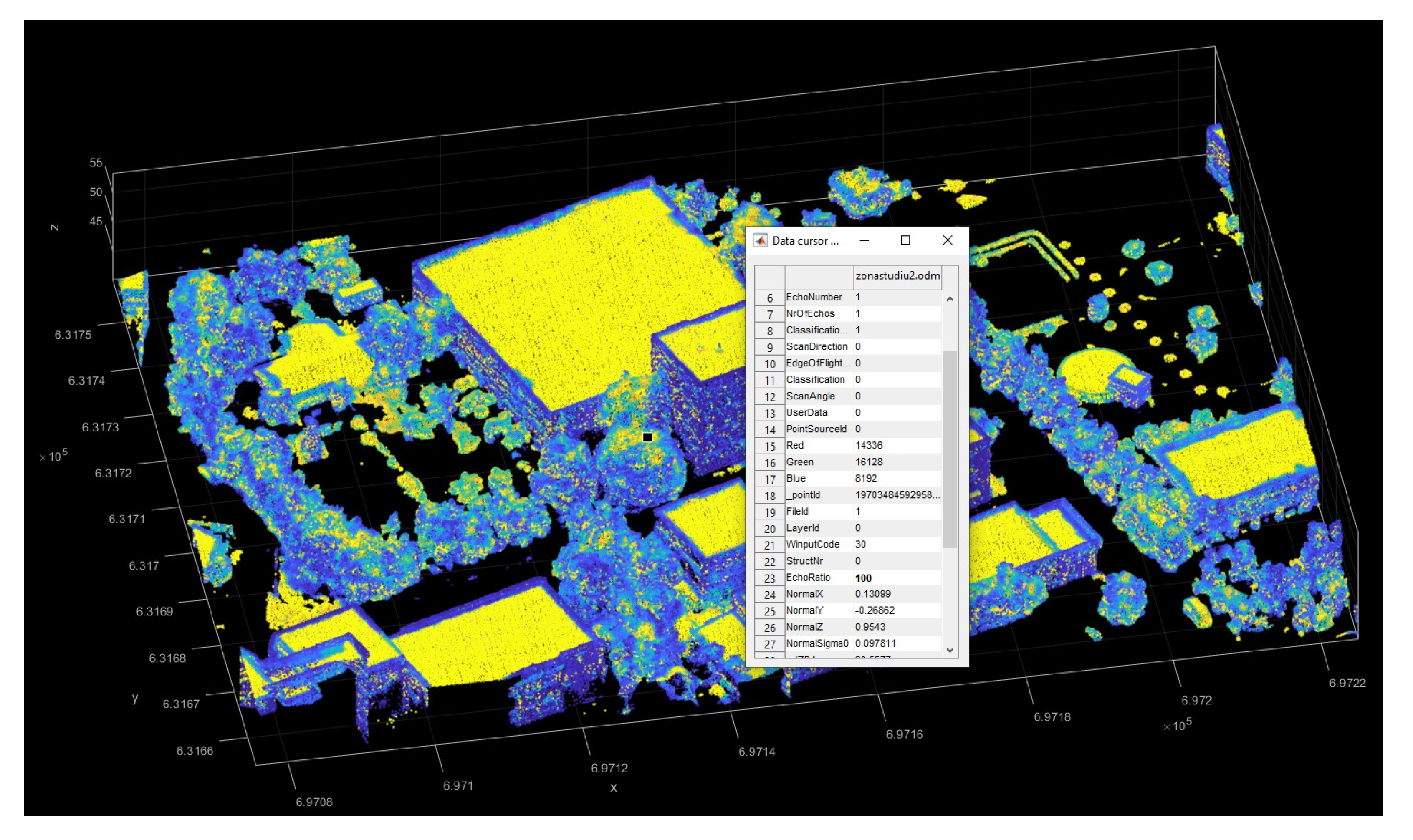
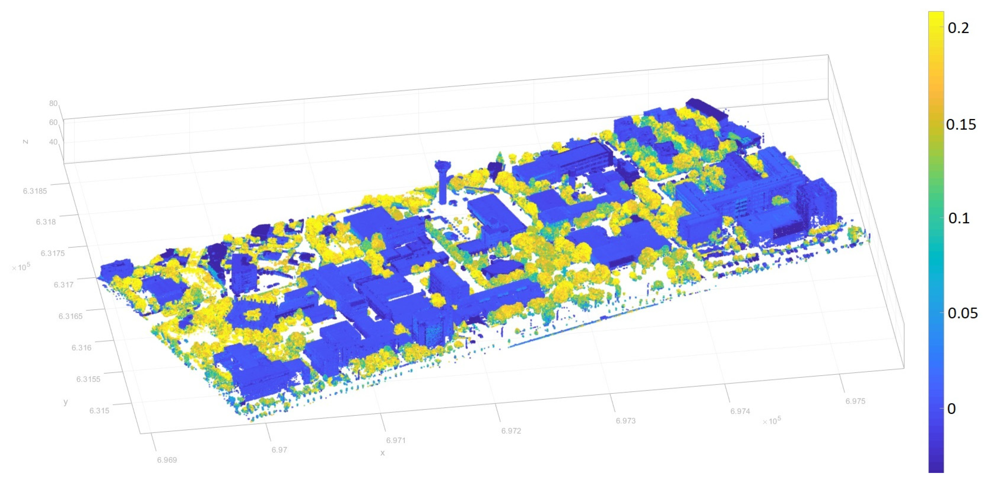
4.3.4. Attributes Computation (Feature Extraction) for Each UAS Point
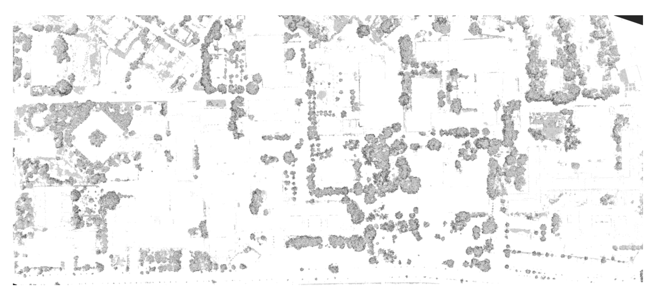
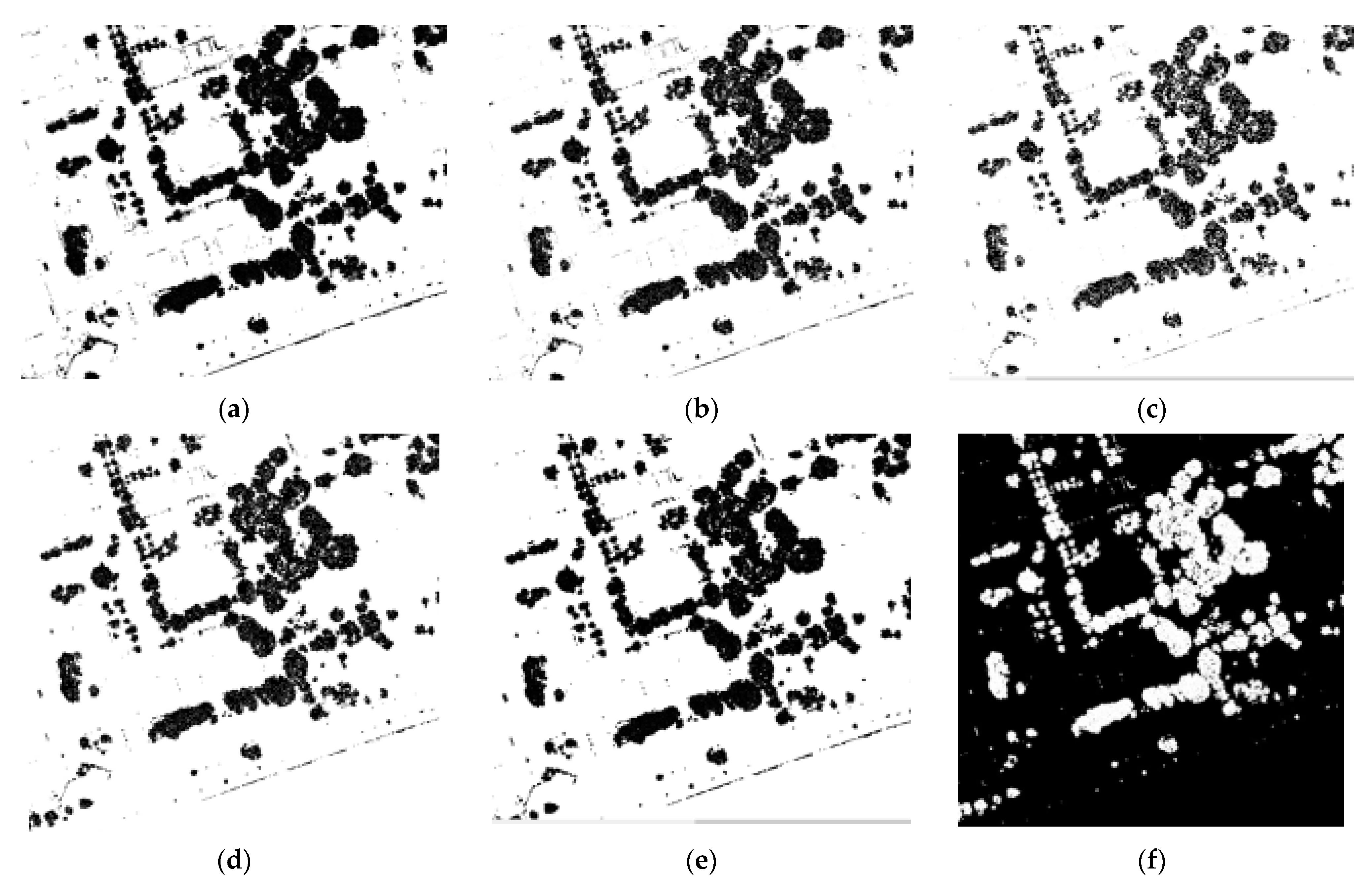
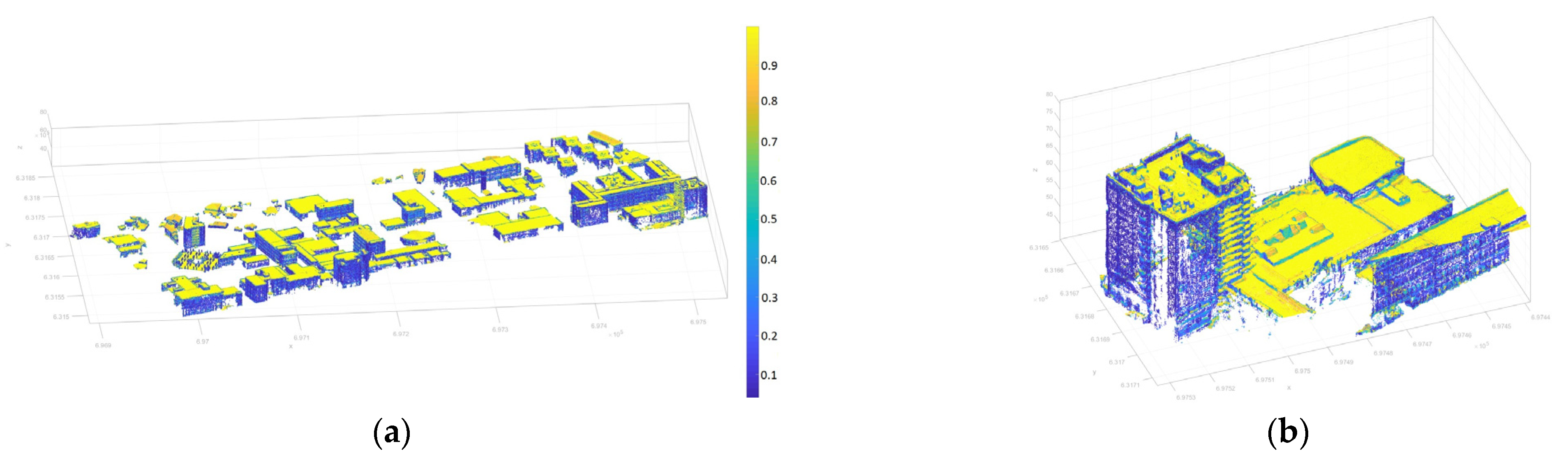
4.3.5. UAS Point Cloud Filtering Using Point Attributes
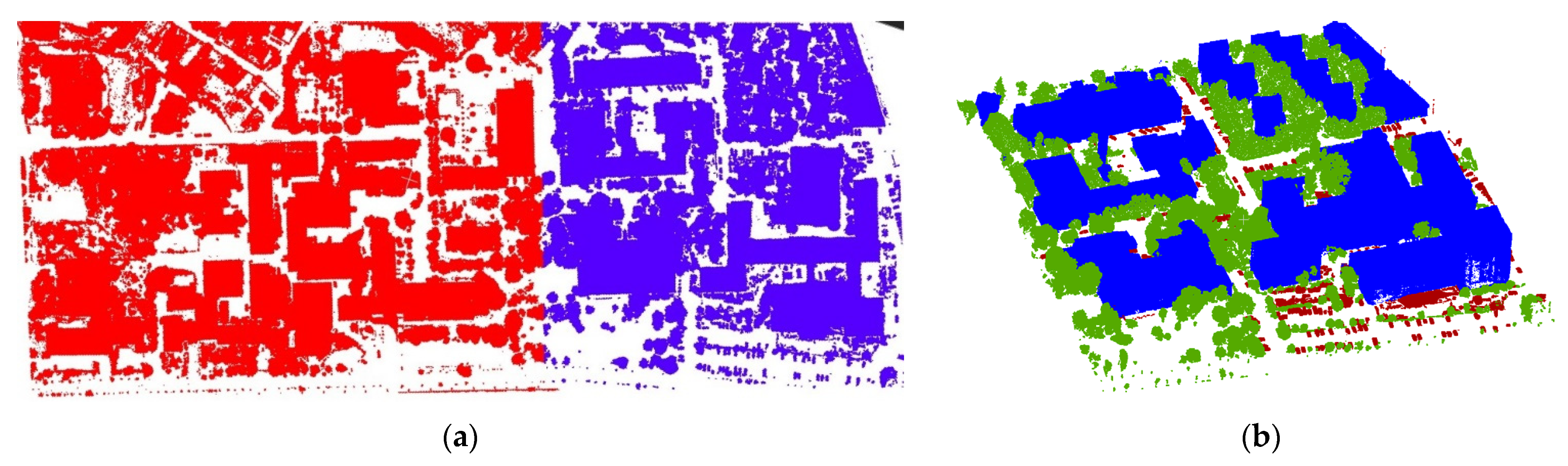
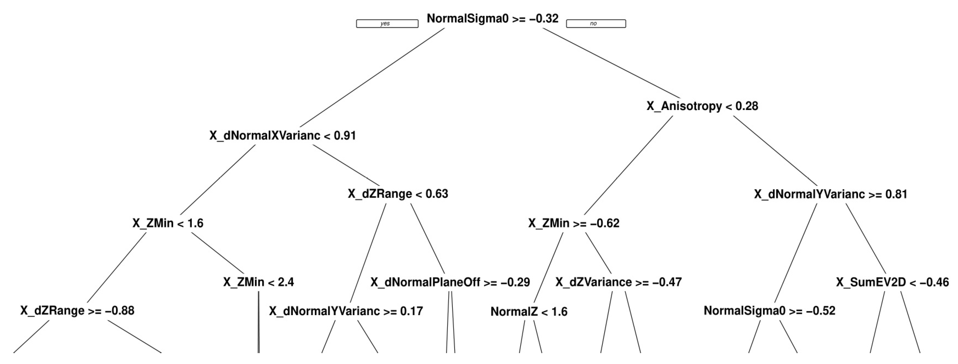
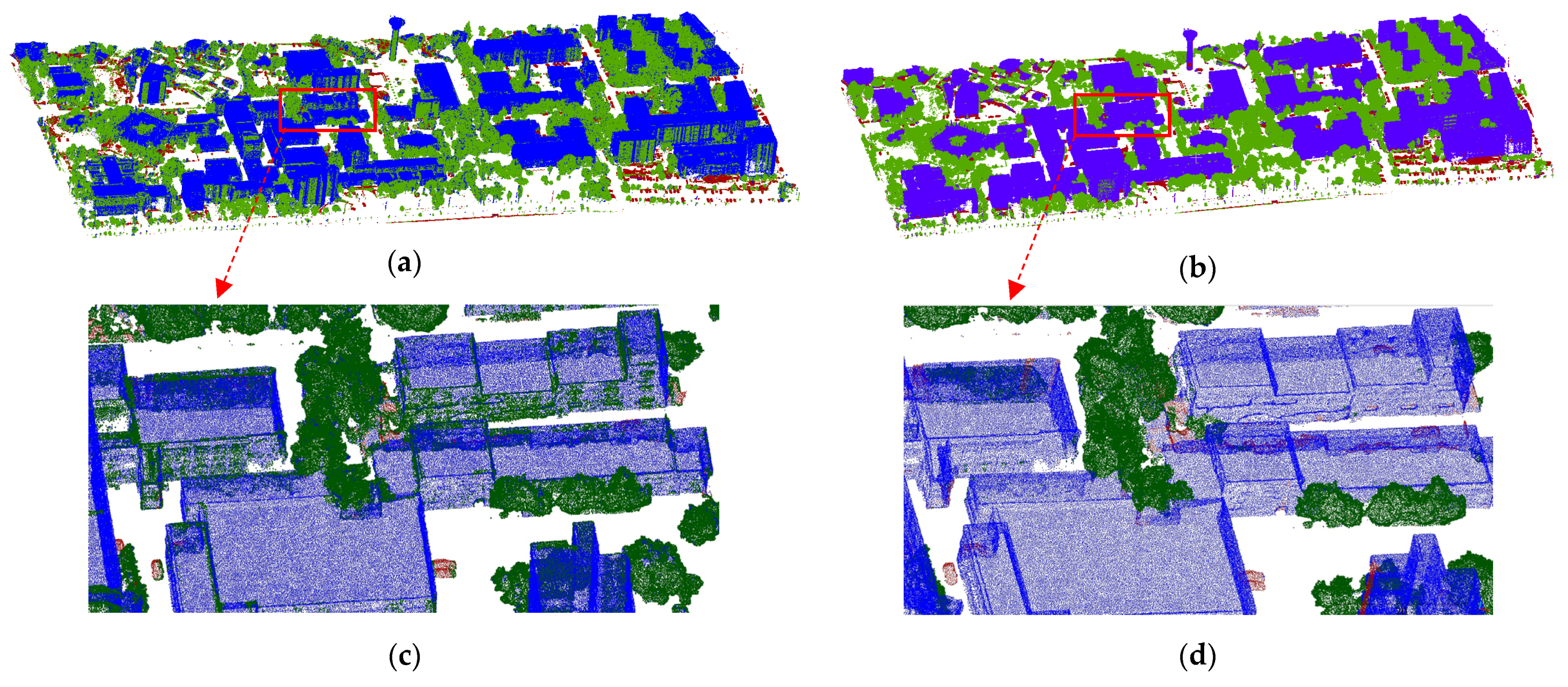
4.3.6. UAS Point Cloud Classification Using Supervised Machine Learning Algorithms
- –
- supervised: based on a training data set, a trained model is obtained, which is applied on the entire data set to label each class;
- –
- unsupervised: the data set is classified without user interaction;
- –
- interactive: the user is actively involved in the classification process through feedback signals, which can improve the results of the classification.
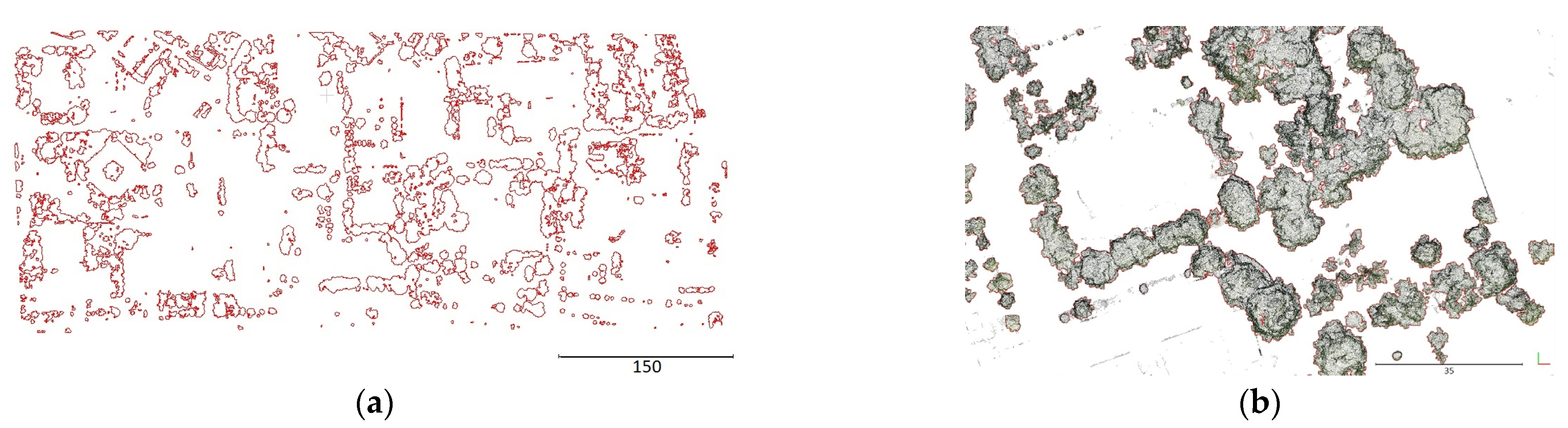
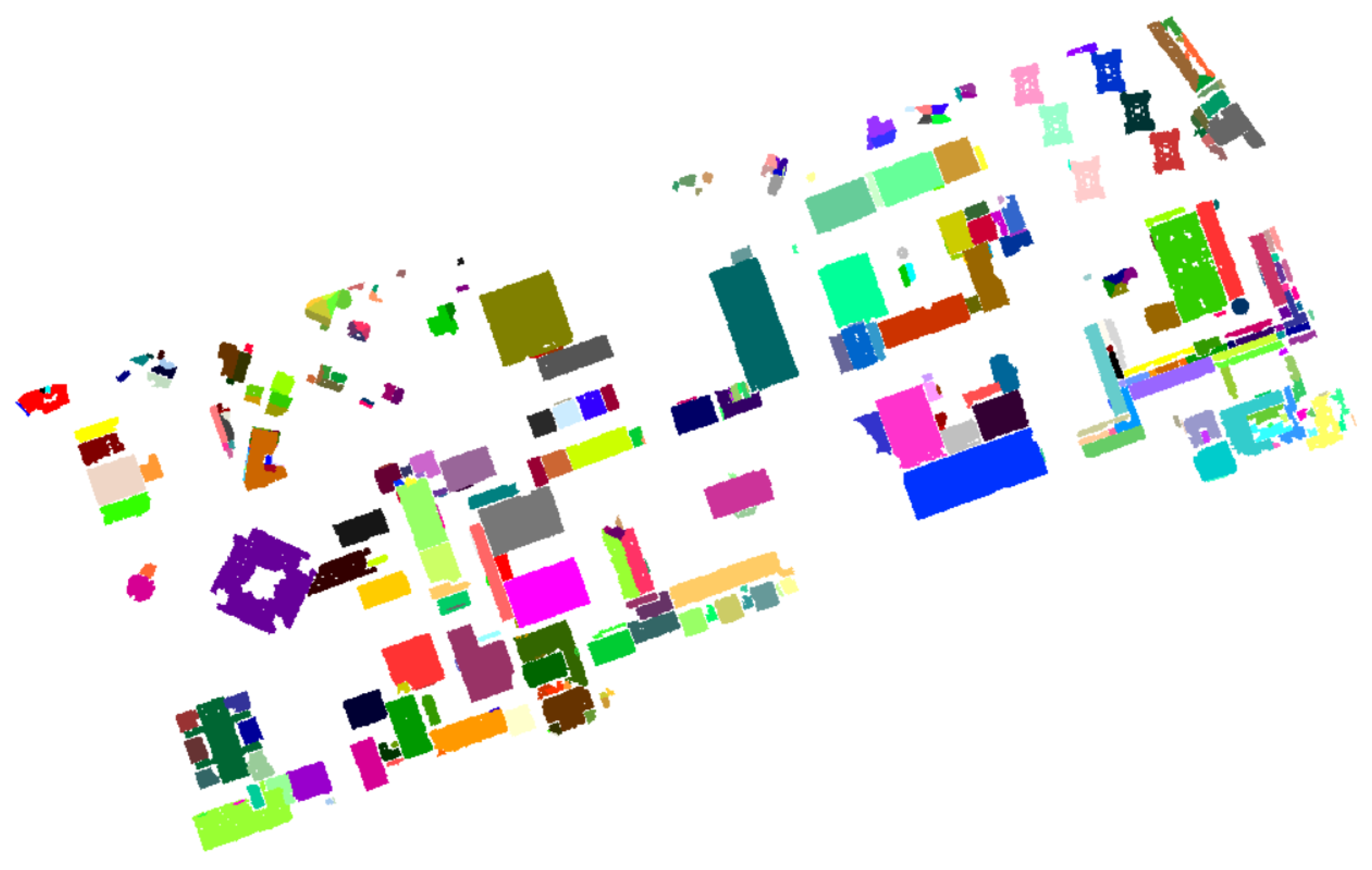
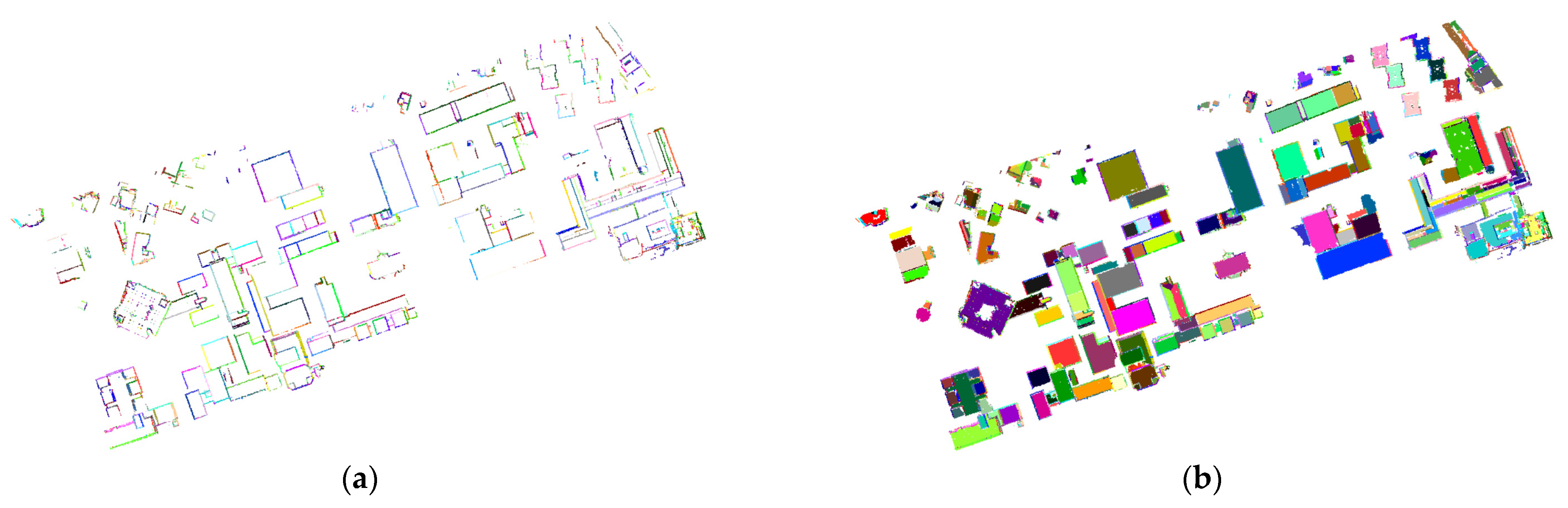
4.3.7. UAS Buildings Point Cloud Segmentation
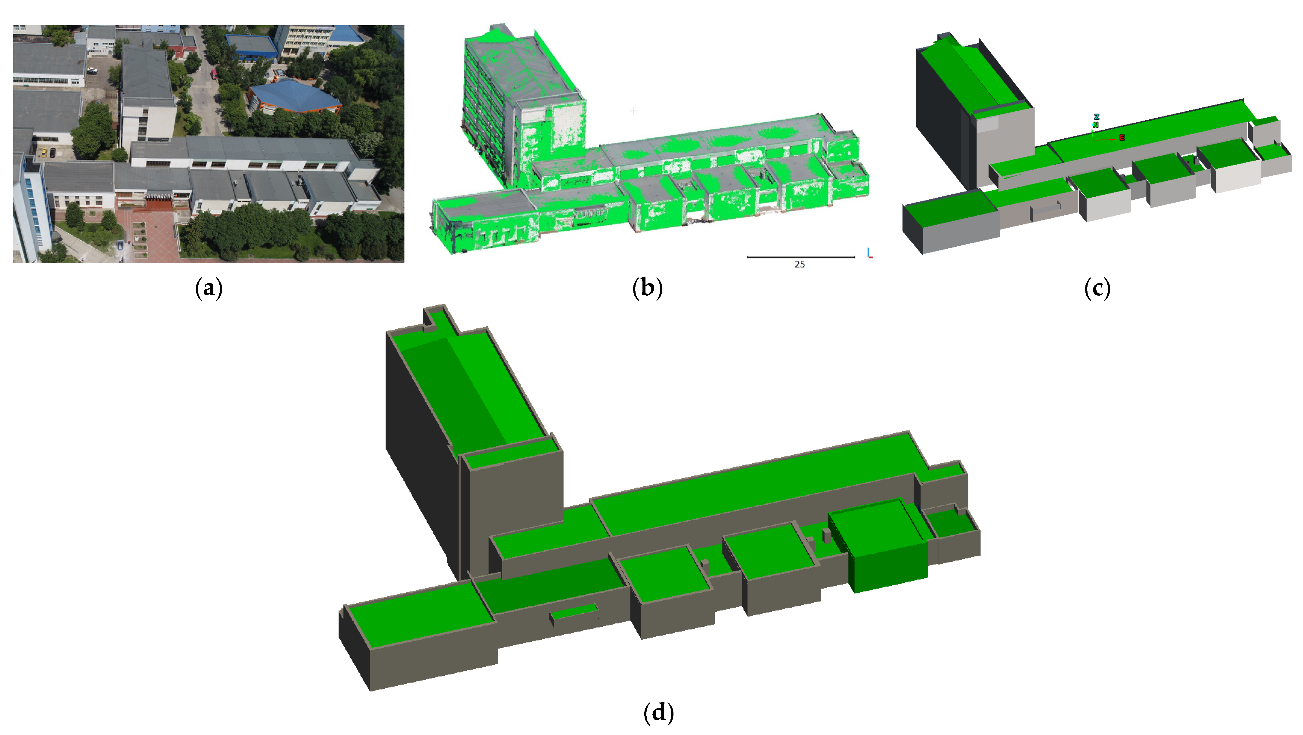
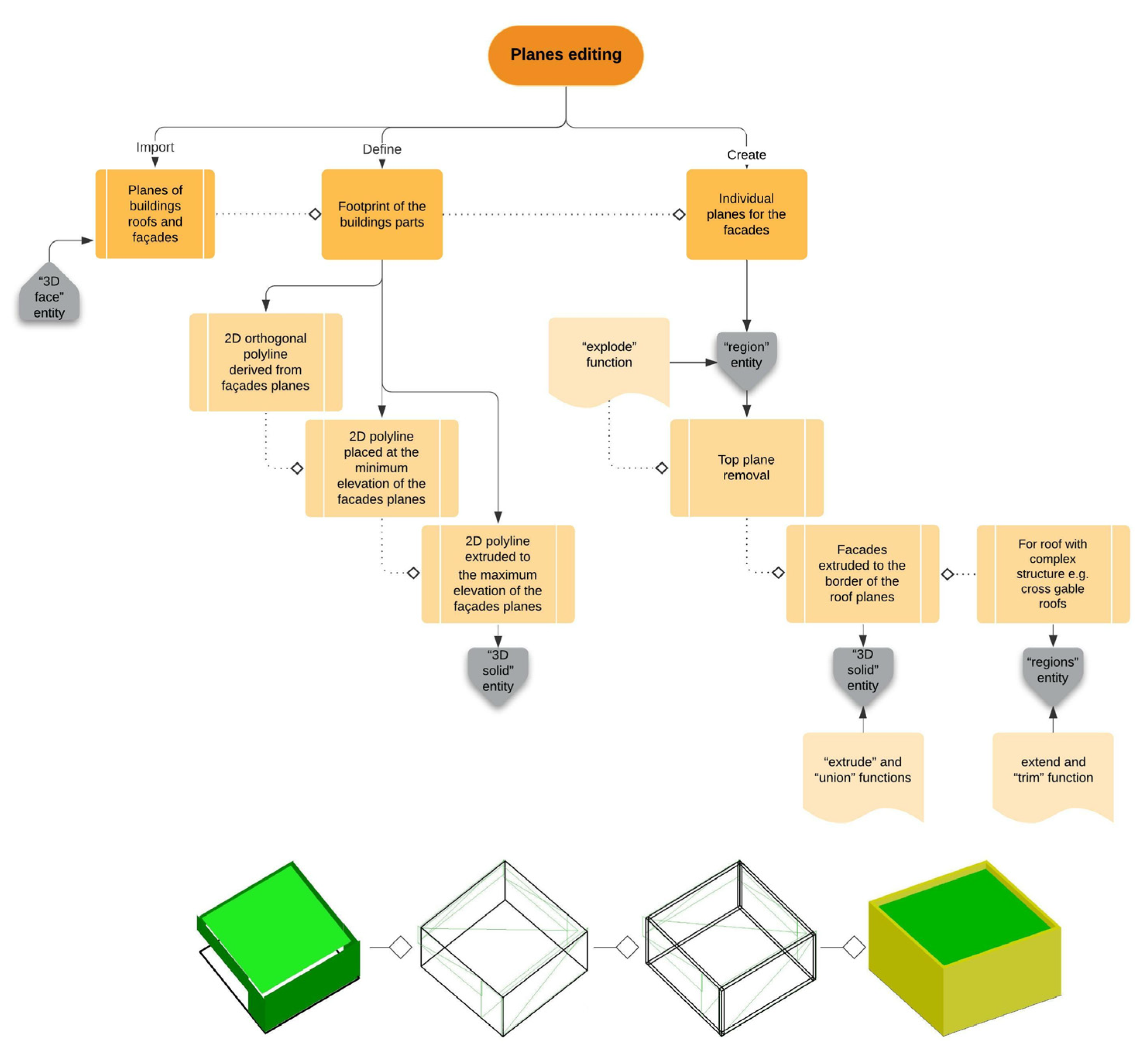
4.3.8. 3D Buildings Model Creation
4.4. Accuracy Assessment of 3D Buildings Models
5. Conclusions
Author Contributions
Funding
Institutional Review Board Statement
Informed Consent Statement
Data Availability Statement
Acknowledgments
Conflicts of Interest
Appendix A


Appendix B

References
- United Nations. Revision of the World Urbanization Prospects; Population Division of the United Nations Department of Economic and Social Affairs (UN DESA): New York, NY, USA, 2018. [Google Scholar]
- Carneiro, C. Communication and Visualization of 3D Urban Spatial Data Acoording to User Requirements: Case Study of Geneva. Int. Arch. Photogram. Remote Sens. Spatial Inform. Sci. 2008, 37, 631–636. [Google Scholar]
- Lafarge, F. Modèles Stochastiques Pour la Reconstruction Tridimensionnelle D’environnements Urbains. Ph.D Thesis, Ecole Nationale Supérieure des Mines de Paris, Paris, France, 2007. [Google Scholar]
- Drešček, U.; Kosmatin Fras, M.; Tekavec, J.; Lisec, A. Spatial ETL for 3D Building Modelling Based on Unmanned Aerial Vehicle Data in Semi-Urban Areas. Remote Sens. 2020, 12, 1972. [Google Scholar] [CrossRef]
- Boulaassal, H.; Landes, T.; Grussenmeyer, P.; Tarsha-Kurdi, F. Automatic segmentation of building facades using terrestrial laser data. In Proceedings of the ISPRS Workshop on Laser Scanning 2007 and SilviLaser 2007, Espoo, Finland, 12–14 September 2007; pp. 65–70. [Google Scholar]
- Lafarge, F.; Descombes, X.; Zerubia, J.; Deseilligny, M.P. Structural approach for building reconstruction from a single DSM. IEEE Trans. Pattern Anal. 2010, 32, 135–147. [Google Scholar] [CrossRef] [Green Version]
- Kolbe, T.; Groger, G.; Plumer, L. Interoperable Access to 3D City Models, First International Symposium on Geo-Information for Disaster Management; Springer: Delft, The Netherlands, 2005. [Google Scholar]
- Kolbe, T.H. Representing and exchanging 3D city models with CityGML. In 3D Geo-Information Sciences; Zlatanova, S., Lee, J., Eds.; Springer: Berlin, Germany, 2009; pp. 15–31. [Google Scholar] [CrossRef]
- Kutzner, T.; Chaturvedi, K.; Kolbe, T.H. CityGML 3.0: New Functions Open Up New Applications. PFG J. Photogramm. Remote Sens. Geoinf. Sci. 2020, 88, 43–61. [Google Scholar] [CrossRef] [Green Version]
- Löwner, M.O.; Gröger, G.; Benner, J.; Biljecki, F.; Nagel, C. Proposal for a new LOD and multi-representation concept for CityGML. ISPRS Ann. Photogramm. Remote Sens. Spat. Inf. Sci. 2016, 4, 3–12. [Google Scholar] [CrossRef]
- Hammoudi, K. Contributions to the 3D City Modeling: 3D Polyhedral Building Model Reconstruction from Aerial Images and 3D Facade Modeling from Terrestrial 3D Point Cloud and Images. Ph.D. Thesis, Institut Géographique National (IGN), Saint-Mandé, France, 2011. [Google Scholar]
- Dorninger, P.; Pfeifer, N. A comprehensive automated 3D approach for building extraction, reconstruction, and regularization from airborne laser scanning point clouds. Sensors 2008, 8, 7323–7343. [Google Scholar] [CrossRef] [PubMed] [Green Version]
- Rottensteiner, F. Automatic generation of high-quality building models from LiDAR data. IEEE Comput. Graph. Appl. 2003, 23, 42–50. [Google Scholar] [CrossRef] [Green Version]
- Nys, G.-A.; Poux, F.; Billen, R. CityJSON Building Generation from Airborne LiDAR 3D Point Clouds. ISPRS Int. J. Geo-Inf. 2020, 9, 521. [Google Scholar] [CrossRef]
- Murtiyoso, A.; Veriandi, M.; Suwardhi, D.; Soeksmantono, B.; Harto, A.B. Automatic Workflow for Roof Extraction and Generation of 3D CityGML Models from Low-Cost UAV Image-Derived Point Clouds. ISPRS Int. J. Geo-Inf. 2020, 9, 743. [Google Scholar] [CrossRef]
- Mwangangi, K. 3D Building Modelling Using Dense Point Clouds from UAV. Master Thesis, University of Twente, Enschede, The Netherlands, March 2019. [Google Scholar]
- Xiong, B.; Oude Elberink, S.; Vosselman, G. Building modeling from noisy photogrammetric point clouds. ISPRS Ann. Photogramm. Remote Sens. Spat. Inf. Sci. 2014, 2, 197–204. [Google Scholar] [CrossRef] [Green Version]
- Xiong, B.; Oude Elberink, S.J.; Vosselman, G. Footprint map partitioning using airborne laser scanning data. ISPRS Ann. Photogramm. Remote Sens. Spat. Inf. Sci. 2016, 3, 241–247. [Google Scholar] [CrossRef] [Green Version]
- Huang, H.; Michelini, M.; Schmitz, M.; Roth, L.; Mayer, H. LOD3 building reconstruction from multi-source images. Int. Arch. Photogramm. Remote Sens. Spatial Inf. Sci. 2020, XLIII-B2-2020, 427–434. [Google Scholar] [CrossRef]
- Pfeifer, N.; Mandlburger, G.; Otepka, J.; Karel, W. OPALS—A framework for Airborne Laser Scanning data analysis. Comput. Environ. Urban Syst. 2014, 45, 125–136. [Google Scholar] [CrossRef]
- 3DFlow 3DF Zephyr Official Web Site. Available online: https://www.3dflow.net/ (accessed on 21 June 2021).
- CloudCompare Official Web Site. Available online: http://www.danielgm.net/cc/ (accessed on 10 June 2021).
- LAStools, Efficient LiDAR Processing Software (unlicensed). Available online: http://rapidlasso.com/LAStools (accessed on 10 June 2021).
- AutoCAD Map 3D v; academic license; Autodesk, Inc.: San Rafael, CA, USA, 2016; Available online: https://www.autodesk.pl (accessed on 19 November 2021).
- Oniga, V.E.; Breaban, A.I.; Pfeifer, N.; Chirila, C. Determining the suitable number of ground control points for UAS images georeferencing by varying number and spatial distribution. Remote Sens. 2020, 12, 876. [Google Scholar] [CrossRef] [Green Version]
- Fan, P.; Li, W.; Cui, X.; Lu, M. Precise and Robust RTK-GNSS Positioning in Urban Environments with Dual-Antenna Configuration. Sensors 2019, 19, 3586. [Google Scholar] [CrossRef] [PubMed] [Green Version]
- Morales, J.; Martínez, J.L.; García-Cerezo, A.J. A Redundant Configuration of Four Low-Cost GNSS-RTK Receivers for Reliable Estimation of Vehicular Position and Posture. Sensors 2021, 21, 5853. [Google Scholar] [CrossRef]
- Gabara, G.; Sawicki, P. Multi-Variant Accuracy Evaluation of UAV Imaging Surveys: A Case Study on Investment Area. Sensors 2019, 19, 5229. [Google Scholar] [CrossRef] [Green Version]
- Xie, P.; Petovello, M.G. Measuring GNSS Multipath Distributions in Urban Canyon Environments. IEEE Trans. Instrum. Meas. 2015, 64, 366–377. [Google Scholar] [CrossRef]
- Lesouple, J.; Robert, T.; Sahmoudi, M.; Tourneret, J.; Vigneau, W. Multipath Mitigation for GNSS Positioning in an Urban Environment Using Sparse Estimation. IEEE Trans. Intell. Transp. Syst. 2019, 20, 1316–1328. [Google Scholar] [CrossRef]
- Rogers, S.R.; Manning, I.; Livingstone, W. Comparing the Spatial Accuracy of Digital Surface Models from Four Unoccupied Aerial Systems: Photogrammetry Versus LiDAR. Remote Sens. 2020, 12, 2806. [Google Scholar] [CrossRef]
- Gašparović, M.; Seletković, A.; Berta, A.; Balenović, I. The evaluation of photogrammetry-based DSM from low-cost UAV by LiDAR-based DSM. South-East Eur. For. SEEFOR 2017, 8, 117–125. [Google Scholar] [CrossRef] [Green Version]
- Piltz, B.; Bayer, S.; Poznanska, A.M. Volume based DTM generation from very high resolution photogrammetric DSMs. Int. Arch. Photogramm. Remote Sens. Spatial Inf. Sci. 2016, 41, 83–90. [Google Scholar] [CrossRef] [Green Version]
- Zhang, W.; Qi, J.; Wan, P.; Wang, H.; Xie, D.; Wang, X.; Yan, G. An Easy-to-Use Airborne LiDAR Data Filtering Method Based on Cloth Simulation. Remote Sens. 2016, 8, 501. [Google Scholar] [CrossRef]
- Štroner, M.; Urban, R.; Lidmila, M.; Kolář, V.; Křemen, T. Vegetation Filtering of a Steep Rugged Terrain: The Performance of Standard Algorithms and a Newly Proposed Workflow on an Example of a Railway Ledge. Remote Sens. 2021, 13, 3050. [Google Scholar] [CrossRef]
- Zhu, L.; Shortridge, A.; Lusch, D. Conflating LiDAR data and multispectral imagery for efficient building detection. J. Appl. Remote Sens. 2012, 6, 063602. [Google Scholar] [CrossRef]
- Weinmann, M.; Schmidt, A.; Mallet, C.; Hinz, S.; Rottensteiner, F.; Jutzi, B. Contextual classification of point cloud data by exploiting individual 3D neigbourhoods. ISPRS Ann. Photogramm. Remote Sens. Spat. Inf. Sci. 2015, 2, 271–278. [Google Scholar] [CrossRef] [Green Version]
- Brodu, N.; Lague, D. 3D terrestrial lidar data classification of complex natural scenes using a multi-scale dimensionality criterion: Applications in geomorphology. ISPRS J. Photogram. Remote Sens. 2012, 68, 121–134. [Google Scholar] [CrossRef] [Green Version]
- Özdemir, E.; Remondino, F.; Golkar, A. An Efficient and General Framework for Aerial Point Cloud Classification in Urban Scenarios. Remote Sens. 2021, 13, 1985. [Google Scholar] [CrossRef]
- Demantké, J.; Mallet, C.; David, N.; Vallet, B. Dimensionality based scale selection in 3D LiDAR point clouds. Int. Arch. Photogram. Remote Sens. Spatial Inform. Sci. 2011, 3812, 97–102. [Google Scholar] [CrossRef] [Green Version]
- Lalonde, J.; Unnikrishnan, R.; Vandapel, N.; Herbert, M. Scale Selection for Classification of Point-Sampled 3-D Surfaces; Technical Report CMU-RI-TR-05-01; Robotics Institute: Pittsburgh, PA, USA, 2015. [Google Scholar]
- Höfle, B.; Mücke, W.; Dutter, M.; Rutzinger, M.; Dorninger, P. Detection of building regions using airborne LiDAR—A new combination of raster and point cloud based GIS methods. In Proceedings of the GI-Forum 2009-International Conference on Applied Geoinformatics, Salzburg, Austria, 7–10 July 2009; pp. 66–75. [Google Scholar]
- Höfle, B.; Hollaus, M.; Hagenauer, J. Urban vegetation detection using radiometrically calibrated small-footprint full-waveform airborne LiDAR data. ISPRS J. Photogramm. Remote Sens. 2012, 67, 134–147. [Google Scholar] [CrossRef]
- Reitberger, J.; Schnörr, C.; Krzystek, P.; Stilla, U. 3D segmentation of single trees exploiting full waveform LIDAR data. ISPRS J. Photogramm. Remote Sens. 2009, 64, 561–574. [Google Scholar] [CrossRef]
- Wang, X.; Wang, M.; Wang, S.; Wu, Y. Extraction of vegetation information from visible unmanned aerial vehicle images. Trans. Chin. Soc. Agric. Eng. 2015, 31, 152–159. [Google Scholar]
- Grilli, E.; Menna, F.; Remondino, F. A review of point clouds segmentation and classification algorithms. Int. Arch. Photogram. Remote Sens. Spatial Inform. Sci. 2017, 42, 339. [Google Scholar] [CrossRef] [Green Version]
- Coussement, K.; Van den Poel, D. Churn prediction in subscription services: An application of support vector machines while comparing two parameter-selection techniques. Expert Syst. Appl. 2008, 34, 313–327. [Google Scholar] [CrossRef]
- Xue, D.; Cheng, Y.; Shi, X.; Fei, Y.; Wen, P. An Improved Random Forest Model Applied to Point Cloud Classification. IOP Conf. Ser. Mater. Sci. Eng. 2020, 768, 072037. [Google Scholar] [CrossRef]
- Nguyen, A.; Le, B. 3D point cloud segmentation: A survey, 6th IEEE Conference on Robotics, Automation and Mechatronics (RAM). In Proceedings of the 2013 6th IEEE Conference on Robotics, Automation and Mechatronics (RAM), Manila, Philippines, 12–15 November 2013; pp. 225–230. [Google Scholar] [CrossRef]
- Xie, Y.; Tian, J.; Zhu, X.X. Linking Points with Labels in 3D: A Review of Point Cloud Semantic Segmentation. IEEE Geosci. Remote Sens. Mag. 2020, 8, 38–59. [Google Scholar] [CrossRef] [Green Version]
- Fischler, M.A.; Bolles, R.C. Random Sample Consensus: A Paradigm for Model fitting with application to Image Analysis and Automated Cartography. Commun. ACM 1981, 24, 381–395. [Google Scholar] [CrossRef]
- Schnabel, R.; Wahl, R.; Klein, R. Efficient RANSAC for Point-Cloud Shape Detection. Comput. Graph. Forum 2007, 26, 214–226. [Google Scholar] [CrossRef]
- Satari, M.; Samadzadegan, F.; Azizi, A.; Maas, H.G. A Multi-Resolution Hybrid Approach for Building Model Reconstruction from Lidar Data. Photogramm. Rec. 2012, 27, 330–359. [Google Scholar] [CrossRef]
- Rabbani, T.; Van Den Heuvel, F.; Vosselmann, G. Segmentation of point clouds using smoothness constraint. Int. Arch. Photogramm. Remote Sens. Spat. Inf. Sci. 2006, 36, 248–253. [Google Scholar]
- Pöchtrager, M. Segmentierung Großer Punktwolken Mittels Region Growing; Technische Universität Wien: Vienna, Austria, 2016; Available online: http://katalog.ub.tuwien.ac.at/AC13112627 (accessed on 12 November 2021).
- Weidner, U.; Forstner, W. Towards automatic building extraction from high resolution digital elevation models. ISPRS J. Photogram. Remote Sens. 1995, 50, 38–49. [Google Scholar] [CrossRef]


| No. of GCPs | Residuals | ||||
|---|---|---|---|---|---|
| RMSEX [cm] | RMSEY [cm] | RMSEZ [cm] | RMSEX,Y [cm] | RMSET [cm] | |
| 3 | 11.9 | 12.4 | 25.9 | 17.2 | 31.1 |
| 5 | 9.3 | 13.2 | 12.7 | 16.1 | 20.6 |
| 10 | 7.2 | 6.7 | 8.1 | 9.8 | 12.8 |
| 10 + 8 | 7.4 | 6.2 | 8.0 | 9.6 | 12.5 |
| 10 + 10 | 6.7 | 5.8 | 6.5 | 8.8 | 11.0 |
| 20 artificial | 6.7 | 5.6 | 6.7 | 8.7 | 11.0 |
| 20 + 8 | 6.3 | 4.9 | 6.9 | 8.0 | 10.5 |
| 20 + 10 | 6.4 | 5.5 | 6.2 | 8.4 | 10.4 |
| 20 + 8 + 10 | 6.2 | 5.0 | 6.6 | 7.9 | 10.3 |
| 45 | 6.1 | 5.0 | 6.4 | 7.9 | 10.2 |
| 8 exterior | 22.6 | 34.2 | 38.1 | 41.0 | 55.9 |
| Interpolation Method | Standard Deviation [m] | ||
|---|---|---|---|
| 0.6 m Search Radius, 20 Neighbours | 1 m Search Radius, 20 Neighbours | 1 m Search Radius, 50 Neighbours | |
| Snap grid | 0.0473 | 0.0473 | 0.0473 |
| Nearest neighbour | 0.0429 | 0.0429 | 0.0429 |
| Delaunay triangulation | 0.0402 | 0.0402 | 0.0402 |
| Moving average | 0.0338 | 0.0333 | 0.0306 |
| Moving planes | 0.0358 * | 0.0355 * | 0.0314 * |
| Robust moving planes | 0.0356 | - | - |
| Moving paraboloid | 0.0419 * | 0.0419 * | 0.0377 |
| Kriging | 0.0339 | 0.0335 | 0.0311 |
| Height-Based Attributes | Formula | Echo-Based Attributes | Formula |
|---|---|---|---|
| NormalizedZ | EchoRatio | ||
| Zmin | |||
| Delta Z | Eigenvalues-based attributes | ||
| Range | Linearity | ||
| Rank | relative height in the neighborhood | Planarity | |
| Height Variance | variance of all Z values in the neighborhood | Anisotropy | |
| Local plane-based attributes | Omnivariance | ||
| Normal vector | NormalX, NormalY, NormalZ | Eigenentropy | |
| Standard dev. of normal vector estimation | NormalSigma0 | Scatter | |
| Variance of normal vector components | Variance of NormalX, NormalY, NormalZ | Sum of eigenvalues | |
| Offset of normal plane | |||
| Sigma X | σX | Change of Curvature | |
| Sigma Y | σY | EV2Dratio | |
| Sigma Z | σZ | Sum of eigenvalues in 2D space | |
| Verticality | 1-normalZ | ||
| Points density |
| Training Data Set | Number of Points | Percent |
|---|---|---|
| Building | 835,631 | 42.8 |
| Vegetation | 675,687 | 52.9 |
| Others | 68,261 | 4.3 |
| Total | 1,579,579 | 100 |
| Vegetation | Building | Others | Sum_Ref. | EoC | Completeness | |
|---|---|---|---|---|---|---|
| Vegetation | 39.7 | 2.5 | 0.5 | 42.8 | 7.1 | 92.9 |
| Building | 3.7 | 49.0 | 0.2 | 52.9 | 7.4 | 92.6 |
| Others | 0.8 | 0.3 | 3.3 | 4.3 | 24.7 | 75.3 |
| Sum_estim. | 44.2 | 51.8 | 4.0 | 100 | ||
| EoC | 10.2 | 5.4 | 18.9 | |||
| Correctness | 89.8 | 94.6 | 81.1 |
| Vegetation | Building | Others | Sum_Ref | EoC | Completeness | |
|---|---|---|---|---|---|---|
| Vegetation | 42.1 | 0.6 | 0.1 | 42.8 | 1.5 | 98.5 |
| Building | 1.0 | 51.3 | 0.6 | 52.9 | 3.1 | 96.9 |
| Others | 0.3 | 0.3 | 3.7 | 4.3 | 14.6 | 85.4 |
| Sum_estim | 43.4 | 52.2 | 4.4 | 100 | ||
| EoC | 3.0 | 1.8 | 15.6 | |||
| Correctness | 97.0 | 98.2 | 84.4 |
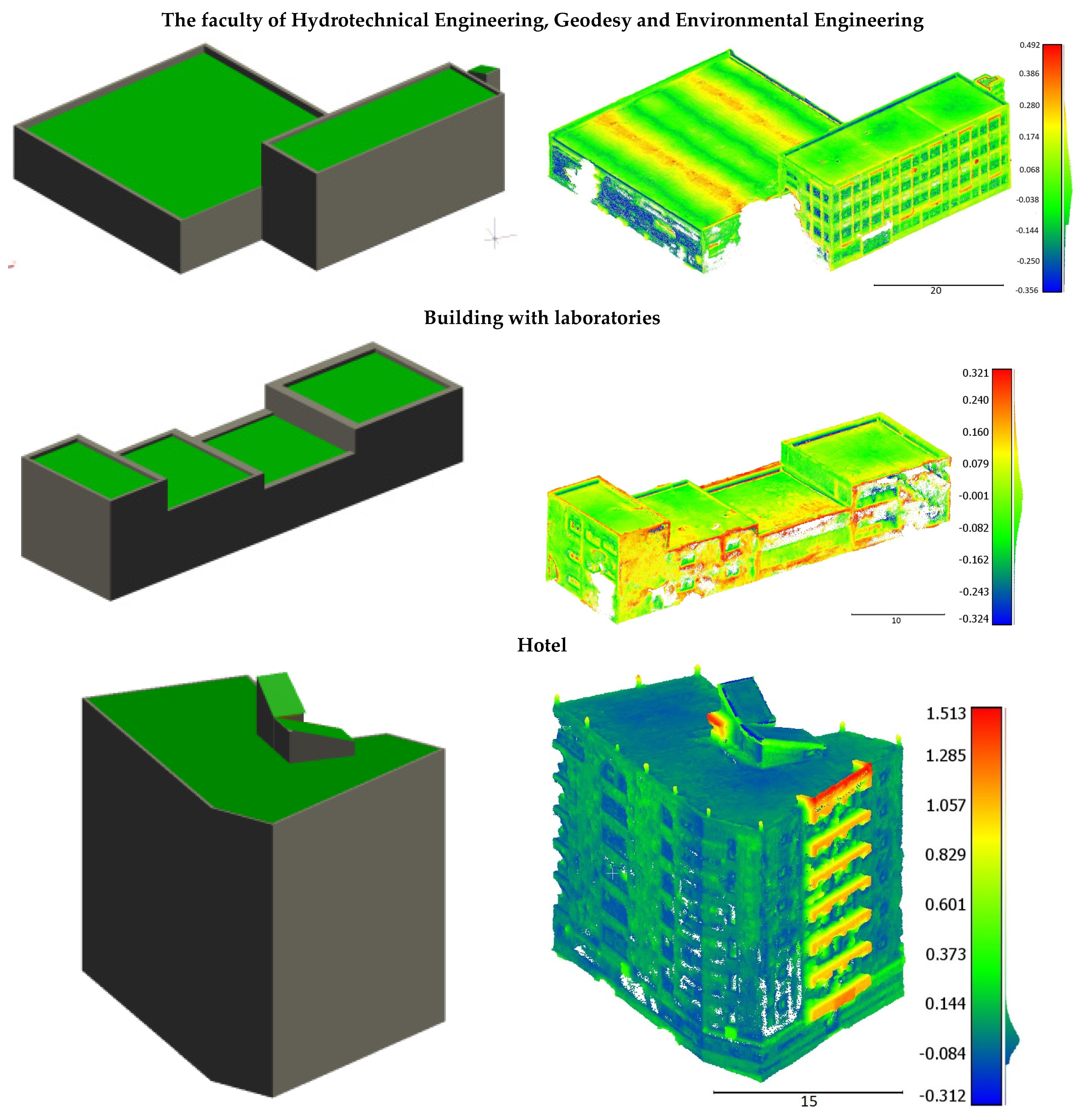
| Building | Standard Deviation Computed Based on Original Point Clouds σ [cm] | Standard Deviation Computed Based on GNSS Points σ [cm] | No. of GNSS Points |
|---|---|---|---|
| Our faculty building | 13.3 | 25.6 | 5 |
| Laboratories | 10.7 | 29.2 | 6 |
| Rectory | 11.9 | 24.4 | 10 |
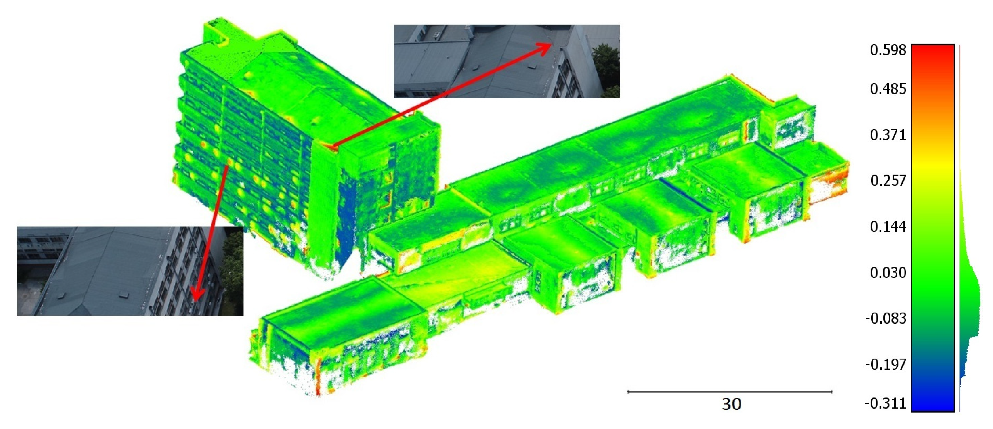
| Hotel | 24.6 (with balconies) 8.4 (without balconies) | - | - |
Publisher’s Note: MDPI stays neutral with regard to jurisdictional claims in published maps and institutional affiliations. |
© 2022 by the authors. Licensee MDPI, Basel, Switzerland. This article is an open access article distributed under the terms and conditions of the Creative Commons Attribution (CC BY) license (https://creativecommons.org/licenses/by/4.0/).
Share and Cite
Oniga, V.-E.; Breaban, A.-I.; Pfeifer, N.; Diac, M. 3D Modeling of Urban Area Based on Oblique UAS Images—An End-to-End Pipeline. Remote Sens. 2022, 14, 422. https://doi.org/10.3390/rs14020422
Oniga V-E, Breaban A-I, Pfeifer N, Diac M. 3D Modeling of Urban Area Based on Oblique UAS Images—An End-to-End Pipeline. Remote Sensing. 2022; 14(2):422. https://doi.org/10.3390/rs14020422
Chicago/Turabian StyleOniga, Valeria-Ersilia, Ana-Ioana Breaban, Norbert Pfeifer, and Maximilian Diac. 2022. "3D Modeling of Urban Area Based on Oblique UAS Images—An End-to-End Pipeline" Remote Sensing 14, no. 2: 422. https://doi.org/10.3390/rs14020422