Article

Integration of Hyperspectral and Magnetic Data for Geological Characterization of the Niaqornarssuit Ultramafic Complex in West-Greenland

1
Faculty of Science and Technology, Norwegian University of Life Sciences, PB 5003, 1430 Aas, Norway
2
Geological Survey of Denmark and Greenland, 1350 Copenhagen, Denmark
3
Rad.Data, 14482 Potsdam, Germany
4
German Research Centre of Geosciences, Telegrafenberg, 14473 Potsdam, Germany
5
Institute of Geosciences, University of Potsdam, 14476 Potsdam, Germany
6
Helmholtz Centre for Environmental Research, 04318 Leipzig, Germany
*
Author to whom correspondence should be addressed.
Remote Sens. 2022, 14(19), 4877; https://doi.org/10.3390/rs14194877
Submission received: 18 August 2022 / Revised: 23 September 2022 / Accepted: 25 September 2022 / Published: 29 September 2022
(This article belongs to the Special Issue New Trends on Remote Sensing Applications to Mineral Deposits)

Abstract

:
The integration of imaging spectroscopy and aeromagnetics provides a cost-effective and promising way to extend the initial analysis of a mineral deposit. While imaging spectroscopy retrieves surface spectral information, magnetic responses are used to determine magnetization at both shallower and greater depths using 2D and 3D modeling. Integration of imaging spectroscopy and magnetics improves upon knowledge concerning lithology with magnetic properties, enhances understanding of the geological origin of magnetic anomalies, and is a promising approach for analyzing a prospective area for minerals having a high iron-bearing content. To combine iron diagnostic information from airborne hyperspectral and magnetic data, we (a) used an iron absorption feature ratio to model pseudo-magnetic responses and compare them with the measured magnetic data and (b) estimated the apparent susceptibility along the surface by some equivalent source modeling, and compared them with iron ratios along the surface. For this analysis, a Modified Iron Feature Depth index was developed and compared to the surface geochemistry of the rock samples in order to validate the spectral information of iron. The comparison revealed a linear increase in iron absorption feature depths with iron content. The analysis was performed by empirically modeling the statistical relationship between the diagnostic absorption features of hyperspectral (HS) image spectra of selected rock samples and their corresponding geochemistry. Our results clearly show a link between the spectral absorption features and the magnetic response from iron-bearing ultra/-mafic rocks. The iron absorption feature ratio of Fe3+/Fe2+ integrated with aeromagnetic data (residual magnetic anomaly) allowed us to distinguish main rock types based on physical properties. This separation matches the lithology of the Niaqornarssuit complex, our study area in West Greenland.

Graphical Abstract

1. Introduction

In harsh environments such as in the Arctic, conventional mineral exploration techniques are challenging due to inaccessibility and remoteness. Optical remote sensing and airborne geophysics offer cost- and time-efficient tools to analyze mineral deposits based on physical properties. Datasets from such methods typically cover large areas and provide physical parameter information which enables the spatial description of the structural and lithological conditions. This makes these methods particularly attractive in an early exploration phase.
However, ore-formation typically involves several processes, and deposits are often hosted in complex background geology and may be overprinted by subsequent tectonic or alteration processes. Therefore, it is rarely the case that a single physical parameter is a diagnostic criterion for the mineralization and that a single method sufficiently describes a deposit. Optical remote sensing and geophysical methods should be combined to address these limitations since consideration of several physical parameters can significantly impact a more successful mineral exploration [1,2].
The key component of the integration of magnetic and optical remote sensing with lithological information is iron. Iron is the most relevant element since (1) a few iron minerals are almost exclusively responsible for the overall magnetic properties of rocks and, hence, anomalies measured in magnetic data, and (2) iron alteration minerals have strong absorption features in multi-/hyperspectral data.
Magnetizations in rocks are mainly associated with ferromagnetic magnetite, other iron-titanium oxide minerals, and the monoclinic sulfide pyrrhotite [3]. This makes magnetic measurements attractive for targeting several mineral deposits containing Fe-oxides and sulfides [4,5]. However, most other minerals, including the alteration minerals of iron (goethite, hematite), have no significant magnetic properties, so a comprehensive lithological characterization is hardly possible based on magnetic data alone.
Magnetite has no characteristic spectral absorption features in the solar-reflective spectral range. However, its presence can be estimated from Fe-alteration products, which show more distinct spectral signatures [5,6]. The transformation of goethite and hematite to magnetite was observed during laboratory heating experiments [7,8,9]. Another limiting factor in an accurate geological analysis is that in many regions either the bedrock is not fully exposed (e.g., partly covered by vegetation or soil layer) or the exposed bedrock surface is primarily covered by lichens [10] as is common in the Arctic. Such lichen coverage can lead to misidentification in the spectra and strongly hampers the mineral and rock composition mapping from the spectral analysis [11,12].
Magnetic data might help to overcome the optical analysis limitations at the rock surface in such cases. It enables tracing geological trends in areas where the information from HS sensors is vague due to full or partial coverage of the rock surface by other materials. Integration of the two methods would also assist in the assignment of magnetic properties to the mineralogy and rock types by geologically contextualizing the magnetic data.
Despite many integration approaches combining optical remote sensing methods (e.g., HS sensors with different spectral ranges [13,14,15,16,17], HS with LiDAR [18,19], or HS with photogrammetry [20,21]), only a little research has been done to combine datasets from the two groups (optical remote sensing and airborne/UAV geophysics) at the interpretation stage for geological applications [22,23]. However, especially for ultramafic/mafic complexes exhibiting distinct magnetic properties, the data integration of airborne magnetic and hyperspectral (HS) imagery (HSM integration) appears to be particularly meaningful in improving the knowledge about lithology.
Most applications combining such methods are seen in areas where bedrock is well-exposed and only sparsely covered by vegetation, such as desert, high-alpine, or arctic environments, and where both magnetic surveys and HS data of high resolution and good quality exist at the same time. Geological characterization with HS data is possible in most of these areas [12,24,25,26,27,28,29,30] because the bedrock is often well-exposed and is only slightly covered by vegetation. Moreover, HS data allows a general mineralogical characterization of the rock surface and can contribute to closing the gap of missing lithological information. Many mineral exploration areas have been uniformly covered with HS airborne surveys and local helicopter-borne magnetic surveys with dense line spacing (<200 m).
Although an HSM integration can provide largely complementary information about the mineralogical composition and appears promising for several mineral exploration target types in many regions, few papers have been published on where data from these methods are combined [2,23,31,32].
This is likely due to the fact that the proper integration of HS and magnetic data is not straightforward for several reasons. First, the measured magnetic responses are generated by magnetization in the whole sub-surface and not only by its near-surface contributions. Furthermore, the magnetic method is known to have a low resolution, such that the exact position and distribution of the magnetization in the ground cannot be determined without additional information, and an infinite number of magnetization distributions in the subsurface can describe the measured data response. This means that without general assumptions about how the magnetization is distributed in the ground, it is challenging to compare magnetics with HS properties at the surface reliably. This situation is further complicated by the fact that magnetization is a vector quantity. This vector quantity consists of an induced component parallel to the current Earth’s magnetic field and a remanent component that can point in a different direction and reflects the Earth’s magnetic field direction when rocks were formed and/or overprinted.
Therefore, it is expected that a simple comparison of data responses presented as magnetic maps (typically given as residual magnetic anomaly) with image products from the HS can only coarsely describe the relationships of magnetic and HS properties on the ground. This is particularly true if magnetic surveys are gathered at greater flight heights and wider line spacings, or when the geology is complex and varies over short distances, or the remanent magnetization component is strong and points in a largely different direction than the induced magnetization.
A plausible future solution for this problem could be to develop magnetic modeling or inversion schemes, where the HS information is incorporated as constraining information along the surface. Such approach would improve the resolution of the magnetics at the surface and, hence, make the magnetization directly comparable to the hyperspectral image results at each pixel. This would allow for a reliable presentation of the relationships between hyperspectral image products and magnetizations in scatterplots and the use of these as inputs in statistical analysis. However, to develop such schemes, it must first be investigated how spectral and magnetic properties are related to each other, such that a geologically reasonable constraint can be found that links the two datasets with each other.
This contribution aims to investigate if it is generally possible to gain more geological information from mineral exploration sites and iron-bearing ultramafic complexes in particular by combining airborne magnetic and HS data. In this contribution, we make the first step in developing an approach to integrating airborne HS and magnetic data properly. We apply an HSM integration using simple forward modeling and inversion tests—fully aware of their limitations. In particular, we compare the resulting apparent magnetic susceptibility estimates along the surface with iron ratios determined from the HS data to make a geological characterization in terms of Fe-mineral variations. The study is supplemented with hyperspectral laboratory and geochemical measurements on rock samples which helps to validate the observed relationships of the different physical parameters in the airborne data and link them to mineralogical knowledge.

2. Study Area—The Niaqornarssuit Complex

As a test area, we selected the intrusive Niaqornarssuit Complex located within the southernmost part of the Paleoproterozoic Nagssugtoqidian Orogen in West Greenland (66.83°N, −52.02°E) which is explored for disseminated Ni and Cu sulfide mineralizations [33]. The area is fully covered both with a regional airborne hyperspectral survey (HyMAP [29]) and a local high-resolution helicopter-borne magnetic survey [34]. The rocks in the complex are largely exposed at the surface, such that it satisfies the conditions to test the integration of HS and magnetic data properly.
The Niaqornarssuit Complex formed in the Palaeoproterozoic from 2050 to 1750 Ma [35] is a layered ultramafic intrusion hosted in Archean gneisses. It is elliptically shaped with a long axis of 1.8 km striking east-west, and a short axis measuring 0.9 km [36]. The complex is a peridotite lens consisting mainly of two homogeneous yellowish-green weathered dunite bodies separated by a thin olivine-poorer peridotite zone with lherzoliteic and harzburgitic composition surrounded by older basement orthogneisses (Figure 1). Some limited observations of intrusive contacts and a significant chilled margin in the southeastern part of the Niaqornarssuit Complex imply that the intrusion was embedded in older basement gneisses of the South Nagssugtoqidian Orogen [33]. The mafic and ultramafic rocks of the study area experienced a metamorphic and tectonic overprint forming the present shape of the complex.
The gently undulating rolling terrain with moderate relief mostly lacks distinct vegetation except in low-lying south-facing slopes and depressions with 1–2 m high shrubs. However, up to 90% of the exposed bedrock surfaces are widely covered by lichens (Figure 2) [12,28,37].
The exploration company 21st North collected more than 160 samples from the complex and defined the stratigraphy of the complex with the following rock units [33]:
(I)
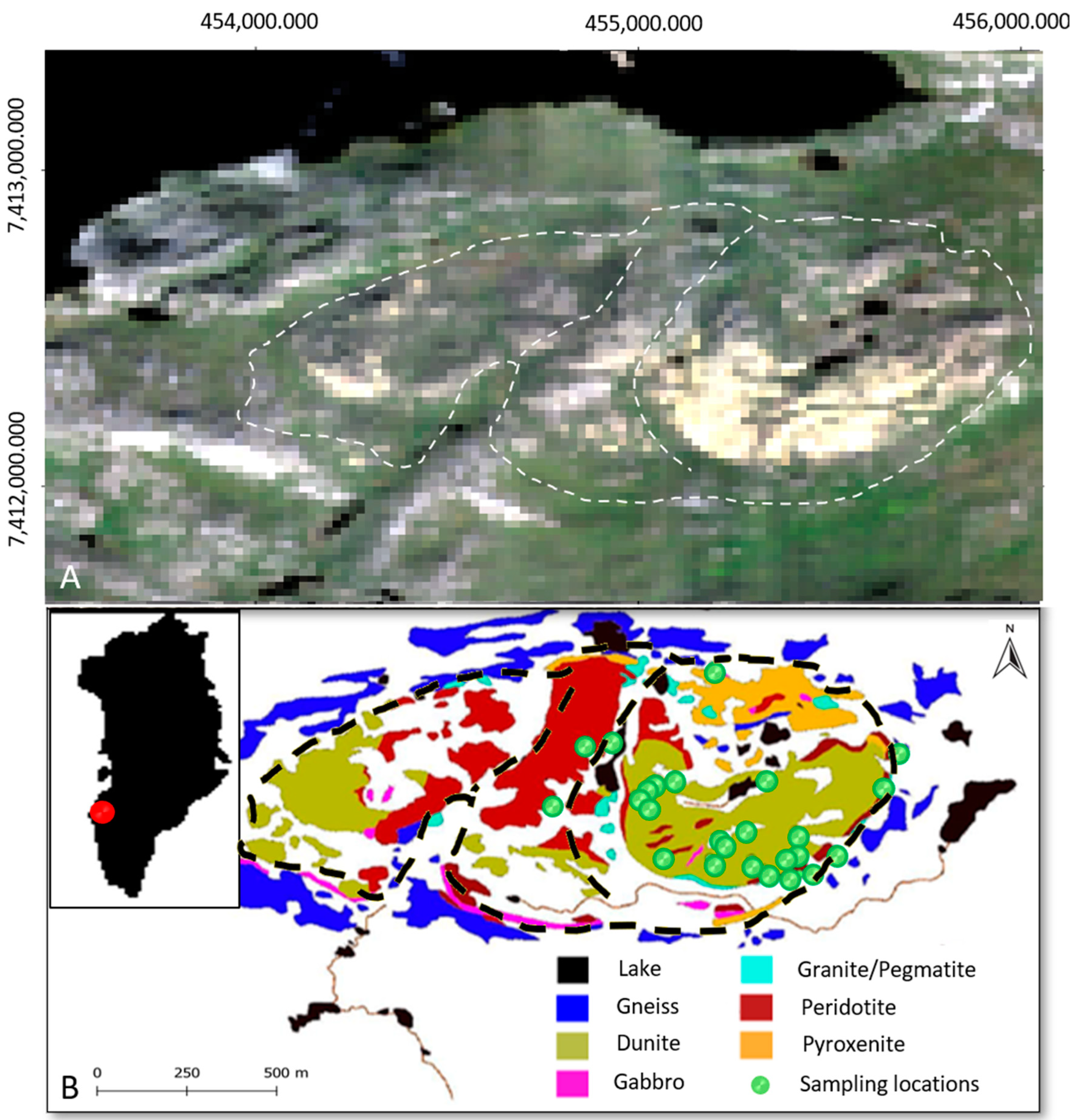
A chilled margin with a black aphanitic-fine-grained peridotite rock composition is located at the contact zone to basement gneisses (navy blue color in Figure 1) and contact-metamorphic granites (light blue color in Figure 1). This formation is 5–30 m thick, sheared, and contains a variable amount of olivine, pyroxene, and oxides;
(II)
A unit with magnetite-chromite-rich homogeneous medium-grained dunite that contains common peridotite-pyroxenite layers and intrusive dikes. The unit is mainly present in two dunite bodies (green beige color in Figure 1);
(III)
A unit that comprises medium- to coarse-grained peridotite olivine-rich at the bottom and pyroxene-rich at the upper level (maroon color in Figure 1);
(IV)
A homogenous unit of coarse-grained to pegmatitic pyroxenite that forms a massive block in the northeastern part of the complex (orange color in Figure 1);
(V)
A discontinuous layer of medium-grained and banded metagabbro (magenta color in Figure 1) interleaved with hornblende-gneiss rocks.
The complex is characterized by strongly weathered gossans and small rusty beds hosted by peridotite and pyroxenite layers at the surface. The weathered zone consists of strongly oxidized malachite-stained gossan boulders. Fresh sulfides such as pentlandite, pyrrhotite, and chalcopyrite are rarely found due to their low resistance to weathering [33,37]. These mineralizations at the surface are almost entirely restricted to the rusty beds of the eastern dunite body.
In this study, the focus of our analysis lies on II (dunite), III (peridotite), and IV (pyroxenite) rock units of the mafic-ultramafic intrusion, and we did not further consider the surrounding host rock (see Section 2). The intrusive rocks mainly consist of mafic minerals (olivine, pyroxene, and amphibole) and minor amounts of felsic minerals and other accessories.
All rock material for our laboratory measurements was collected exclusively from the eastern part of the complex since we used samples from the 21st North that concentrated their investigations on this region showing most ore concentrations.

3. Mafic and Ultramafic Rocks

Ultramafic rocks are the main component of the Earth’s mantle which initially formed when the Earth differentiated into an iron-rich core and a silicate mantle [38]. Peridotites containing more than 40% olivine can be distinguished from pyroxenites characterized by an olivine content of less than 40% [39,40]. Dunites are peridotites with a very high olivine content of more than 90%. Since in this study we are analyzing both peridotites and dunites, for simplicity, peridotites are referred to as peridotites with between 40 and 90% olivine content.
Iron is the common element to characterize ultramafic rocks with optical remote sensing and the chemical element retaining magnetic properties [3]. It is the most common element in the Earth’s crust and is exposed at the Earth’s surface in nearly all rocks, especially in the ultramafic bodies [41] and, hence, well-suited to generally distinguish different lithologies for such ultramafic intrusions. Ferrous iron (Fe2+) mainly occurs in the original mantle minerals such as olivines and pyroxenes [42]. Minerals reacting with water or atmosphere undergo a process of oxidation and alteration, resulting in the formation of iron oxide/hydroxide minerals (ferric iron Fe3+) as hematite (Fe3+2O3), goethite (Fe3+O(OH)), limonite (Fe3+O(OH)∙nH2O), and magnetite (Fe3+2Fe2+O4) [43]. Olivine, the main component of dunite, weathers very quickly and undergoes a serpentinization process under the right atmospheric conditions producing secondary minerals such as serpentines [44].

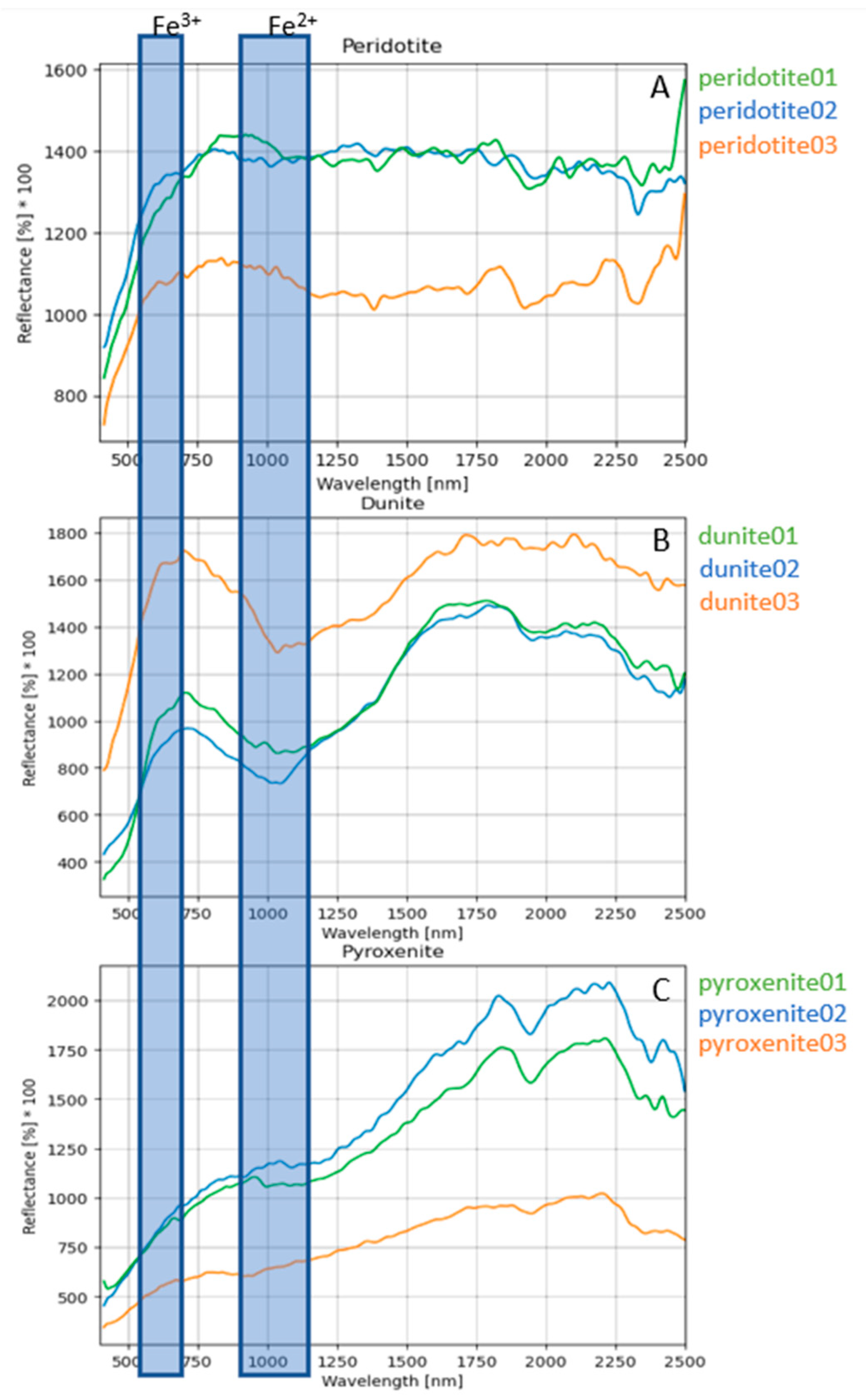
3.1. Spectral Signatures of Ultramafic Rocks

Ferrous (Fe2+) and ferric (Fe3+) iron have distinct absorption features close to 1000 nm and 650 nm, respectively (Figure 3).
However, not all minerals containing iron show distinct absorption features within the spectral range of 400 to 2500 nm (Figure 4), such as magnetite which can be easily confused with, e.g., the Fe-bearing sulfide mineral chalcopyrite. Furthermore, magnetite is an accessory mineral in intrusive rocks and is typically not identifiable in airborne HS data.
The ferrous iron content in the ultramafic rocks is dominant and complies with the higher ferrous absorption bands (close to 1000 nm). For dunite, containing almost all olivine (having iron included as Fe2+), only absorption feature at 1000 nm is exhibited [45]. Altered minerals containing ferric ions in Fe-O by oxidation exhibit a significant fall-off of the reflectance intensity in the UV-blue region (100–400 nm) of the electromagnetic spectrum [45]. Some colored Fe minerals display absorption features in visible light (400–700 nm) called color centers. These spectral characteristics are not caused by the material’s chemistry but by electronic processes [5].
Figure 4. Comparison of chalcopyrite, magnetite, and olivine spectra extracted from the splib07 USGS spectral library [46].
Remotesensing 14 04877 g004
In this study, iron absorption features close to 850 nm related to Fe2+–Fe3+ intervalence charge transfer are not included in the calculations. This band is not indicative of ferrous or ferric iron and overlaps with the absorption feature at 1000 nm.

3.2. Magnetism in Ultramafic Rocks

Ultramafic rocks such as pyroxenites, peridotites, and serpentinized dunites have typically high concentrations of magnetic minerals [4]. Primary ferromagnetic magnetite is the most significant magnetic mineral here, although its content in the rock is relatively low (<1 volume percent) and classified as an accessory. In addition, secondary magnetite forms during the serpentinization process of ultramafic rocks:
3Mg3FeSi2O3 + 6H2O + O → (Mg,Fe)6Si4O10(OH)8 + Fe3O4
Fe-bearing forsterite serpentine magnetite
Ultra-basic rocks with Fe-bearing forsterite and orthopyroxene react with water and are altered to serpentine and secondary magnetite during serpentinization [47]. The secondary magnetite amount is small and non-linearly correlated with the serpentinization degree [48,49]. However, it is relevant in the comprehension of the mechanism and evolution of the upper mantle and lower crust [50]. Magnetism increases with serpentinization until the metamorphic grade of amphibolite facies is reached [51]. At higher grades, ultramafic rocks become deserpentinized, and magnetite disappears due to the replacement of iron by other elements [3].
Since olivine and pyroxene are relatively weakly magnetic (paramagnetic: μ = 12–540 and 12–330, respectively [4]), minerals responsible for features in the spectra are not considered to be mainly responsible for stronger magnetic responses despite the significant content of olivine and pyroxene in mafic rocks [52].

4. Data Acquisition

The dataset consists of several data types analyzed in the HSM-integration approach including airborne and laboratory measurements. The airborne data comprises hyperspectral (HyMAP) and magnetic data (a local helicopterborne survey). The laboratory scale analysis includes HS scans of rock samples from the ultramafic complex using an imaging spectrometer—HySpex, and Laser-Induced Breakdown Spectrometer (LIBS) measurements to obtain the surface geochemistry.

4.1. Airborne Surveys

4.1.1. Magnetic Survey

The magnetic data were acquired as part of a combined time-domain electromagnetic and magnetic helicopter-borne survey in 2012 by Geotech Ltd. from Aurora, Canada, [34], using a horizontal magnetic gradiometer with two cesium magnetometers (Table 1).
The magnetometers were placed on a loop hanging ~24 m below the helicopter and had a horizontal distance of ~12.5 m from each other. A GPS navigation system and a radar altimeter were built-in, allowing to generate a local Digital Elevation Model (DEM) of the terrain. The helicopter flew with an average speed of 80 km/h at a mean altitude of 87 m, such that the magnetic sensors were positioned on average 63 m above the ground. Magnetic data were recorded with a sampling interval of 0.1 s. The split-beam cesium vapor magnetometer had a sensitivity of 0.001 nT. General in-line and tie-line spacings were 200 m and 2000 m, respectively, but the denser in-line spacing of 100 m was used across the mafic intrusion (Figure 5). A combined magnetometer and GPS base station was located at the Kangerlussuaq airport, about 60 km away [33].
The total magnetic intensity map obtained through preprocessing (of the data from the two magnetometers) that included, among others, diurnal corrections and micro-leveling [34], is shown in Figure 5.
Since we focus on near-surface anomalies, we removed the impact of the core field by subtracting the IGRF (International Geomagnetic Reference Field) (box 14 in Figure 6) from these preprocessed data. Finally, we applied a 2-D Butterworth high-pass filter with a cut-off wavelength of 3000 m (filter order of 8) to a grid (cell sizes: 20 × 20 m), which was created from the residual magnetic data points by minimum curvature gridding (box 15 in Figure 6). Afterwards, the filtered values were determined at the measurement locations by means of sampling the grid.
An additional filter to prepare the magnetic data for the HSM integration could be a Reduce-To-Pole transformation that removes the effect of the Earth’s magnetic field direction on the shape of magnetic anomalies from the induced magnetization. We did not apply the Reduce-To-pole correction in this study since the study area is close to the magnetic south pole; hence, the differences are minor, but the correction might be considered for surveys conducted at lower latitudes.

4.1.2. Hyperspectral Survey

The HS HyMAP data were acquired in South West Greenland in 2002 [29] (Table 2).
The whisk-broom sensor was mounted on a Piper Navajo Chieftain aircraft flown ~2500 m above the mean sea level, giving the scanner’s swath width of 3000 m [53,54]. The data comprise 53 flight lines covering 7500 km2. For this study, three flight lines were selected. The geocoded radiance data were converted to at-surface reflectance (box 10 in Figure 6), adjusting illumination levels using ATCOR4 software with rugged terrain optimization [11]. The features associated with atmospheric H2O and OH close to 1400 and 1900 nm bands were excluded for further analysis.
The images with residual 106 channels were mosaicked using ENVI® version 5.6. Moreover, clouds, shadows, water, snow, ice, and steep terrain with low illumination were masked from hyperspectral images. The albedo differences in the atmospherically corrected data are caused by the bidirectional reflectance distribution effects (BRDF) [55], and the atmospheric correction causes the remaining artifacts. The final hyperspectral images had 20 × 20 m pixel sizes later used to discretize magnetic modeling and inversion (see Section 5.2).

4.2. Laboratory Measurements

We used 23 rock samples from the eastern part of the Niaqornarssuit Complex for laboratory measurements (boxes 1 to 9 in Figure 6). The samples represent the main lithological rock types in the study area, including peridotites and pyroxenites. The exact sampling locations for all rocks on a 1:10,000 geological map are shown in Figure 1. All 23 samples were scanned in the hyperspectral laboratory on the weathered sample side to imitate the real acquisition conditions of the airborne HyMap sensor that mainly measured weathered rock surfaces in the study area. In order to obtain the samples’ lithogeochemistry, additional whole-rock analysis was performed.

Spectral Data

In the laboratory, the rock specimens were scanned using two HS imaging spectrometers, HySpex VNIR-1600 and SWIR-320-e sensors (Table 2). Laser-Induced Breakdown Spectrometer (LIBS) was then used to identify and quantify the first few micrometers of the sample surface’s chemical components. LIBS is an analytical technique used to determine the elemental composition of materials. A focused, pulsed laser beam is directed at a sample surface, where laser energy absorption and material ablation produce high-temperature microplasma. Small amounts of the measured material are dissociated and ionized at the laser focal point, and during cooling, atomic/ionic emissions in the plasma are generated. An integrated detector was used to spectrally/temporally detect the plasma signals and record the emission lines of all elements present in the material. The resulting LIBS spectrum represents the complete chemical composition of the analyzed material [56]. LIBS data using the SciAps Z-300 was collected within the 190–950 nm wavelength range. The 50 Hz laser emits 5–6 mJ per pulse and analyzes every element in the periodic table. The LIBS measurements were taken pointwise with a fourfold shot at each homogeneous region where HySpex mean spectra were determined.

5. Proposed Method

The presented integration approach is set up to provide a first analysis suited to characterize exposed iron-rich geologies by a combination of optical and magnetic properties. The whole process chain is depicted in Figure 6. The analysis starts with comparing modified iron feature depths (MIFDs) in the laboratory and lithogeochemical information of rock samples—Result 1. In the next step, the MIFDs calculated from airborne data are compared with the MIFDs of the rock samples on a laboratory scale—Result 2. Then, airborne-based MIFDs image information is combined with airborne magnetic results by applying magnetic modeling and inversion tests. Results from the integrated analysis are finally compared with the lithology of the ultramafic complex—Result 3. It has to be noted that the laboratory results are based on measurements of only 23 rock samples that were distributed within and nearby the eastern dunite body. Therefore, all considerations and discussions are related to this part of the ultramafic complex.

5.1. Preparation of Laboratory Optical Remote Sensing Data

The original laboratory HS raw data in 16-bit integer digital numbers (DN) from the HySpex spectrometer were transformed to radiance, followed by conversion to reflectance data (box 2 in Figure 6) using an in-house algorithm [57]. The approach is an iterative log-polar phase correlation technique based on least square regressions from Averbuch and Keller that reduces spatial non-uniformities and detects the reflection of white [58]. The reflectance retrieval also included a geometric alignment and a leveling adjustment between the HySpex system sensors—VNIR (400–1000 nm) and SWIR (1000–2500 nm) for the spectral overlap region of both sensors (VNIR and SWIR) between 940 and 1000 nm.
The absolute reflectance of laboratory measurements was calculated using the white reference’s whole reflectance spectrum (VNIR and SWIR) [57]. Depending on the target’s albedo, the white reference of 5, 20, 50, 90, or 95% can be chosen to resemble the reflection factor of the sample. In this way, the optimal saturation of the measurement is achieved. The extrapolated irradiance of radiance spectra in all pixels was normalized and built up the reflectance data as output. The calculated reflectance data in the laboratory were adapted to the spectral resolution of the airborne images from HyMap, simulating the HyMap properties in the laboratory (box 3 in Figure 6). The simulated laboratory data were further analyzed applying supervised spectral unmixing (box 4 in Figure 6) to identify the surface component and retrieve the fractional abundance of the pure elements at every pixel of the HS scene in each rock sample.
For spectral unmixing, the Bounded Variable Least-Squares algorithm (BVLS) was applied to find the percentage of each endmember in each pixel, assuming that measured spectra at each pixel are mixtures of different endmembers [59]. The BVLS results in abundance maps. For this approach, a user-defined spectral library was considered that consists of (1) reference spectra that were measured on pure minerals and lichen using the HySpex spectrometer (Table 2) and (2) spectra extracted from the USGS Digital Spectral Libraries: splib06 [60] and splib07a [46].
Next, the Principal Component Analysis (PCA) [61] (box 5 in Figure 6) was applied to the abundance maps to find abundance clusters in each sample. The simulated BVLS results were individually considered in the PCA using the related covariance matrix. The PCA was used to remove the redundancy in the spectral data, extract spectrally homogeneous regions within a sample, and retrieve a mean reflectance spectrum for each abundance cluster (box 6 in Figure 6). The calculated mean spectrum could be more straightforwardly used than the lower-resolution airborne-based data. It was assumed that an airborne pixel spectrum could be considered a spatio-spectral, quasi-linear mixture of multiple millimeter spectra. A PCA-based dimensional reduction of regional unmixing abundances might reflect the fractal scaling property between meter and millimeter pixel spectra, which was required in this study.
After retrieving the mean spectra for each abundance cluster, we used the LIBS device to determine the surface geochemistry of the rock sample’s homogeneous regions (abundance clusters) (box 7 in Figure 6). For this purpose, LIBS was used without a beforehand prepared iron calibration curve. It has to be noted that LIBS does not provide information about ferrous and ferric iron separately. Therefore, we calculated a ratio of the primary mantle elements iron (Fe) to magnesium (Mg) for every spectrum and used it for further analysis (box 8 in Figure 6) to get a semiquantitative result. It has to be noted that for some rock samples, we extracted more than one homogeneous region resulting in multiple LIBS scans on one sample.
A new iron index was developed to relate the iron content from the LIBS measurements with the spectral signatures. Such an index was calculated for each mean spectrum for ferrous (MIFD1000) and ferric iron (MIFD650), respectively (box 9 in Figure 6). We assumed that the depth of absorption feature of a given element increases with the chemical content of that element in the sample.
The new iron index—Modified Iron Feature Depth index (MIFD)—is based on the Iron Feature Depth (IFD) classification tool for hyperspectral data [62], providing the spatial distribution of iron-bearing minerals due to iron absorption features. However, our MIFD uses division instead of subtraction to avoid negative values in ferrous and ferric iron ratios (Equations (2) and (3)) and to suppress remaining micro shadow effects that impact the at-surface reflectance retrieval. The MIFD algorithm is based on the left 𝜆𝑙𝑒𝑓𝑡 and the right shoulder wavelength 𝜆𝑟𝑖𝑔𝑡 of a feature, its absorption center wavelength 𝜆𝑐𝑒𝑛𝑡𝑒𝑟, and corresponding reflectance values 𝑟𝑙𝑒𝑓𝑡, 𝑟𝑟𝑖𝑔𝑡, 𝑟𝑐𝑒𝑛𝑡𝑒𝑟, respectively (Figure 7).
The depth is estimated by setting an interpolated continuum between both shoulders of the absorption feature and calculating the quotient between the interpolated line lineint and given absorption center rcenter by the following formula:
l i n e i n t = r l e f t + ( r r i g h t r l e f t ) λ c e n t e r λ l e f t λ r i g h t λ l e f t
M I F D = l i n e i n t r c e n t e r
For the MIFD retrieval in this study, the iron spectral features close to 1000 nm (related to ferrous iron) and 650 nm (related to ferric iron) are set up as absorption centers (Figure 7).
MIFD650 and MIFD1000 absorption depth estimates were calculated on all 23 rock samples (approximately on two regions of each sample) measured by HySpex and from the airborne HS HyMap image at the ultramafic complex (box 11 in Figure 6). Depending on the optical sensor, the closest bands to 650 nm and 1000 nm are selected as the centers for absorption features 𝑟𝑐𝑒𝑛𝑡𝑒𝑟. The MIFD at 1000 nm is considered as more reliable for airborne-based HS data than the 650 nm band since the 650 nm is positioned close to the end of the spectral region, which may distort the results. In contrast, the MIFD at 650 nm iron feature is more reliable than the one at 1000 nm in the HS data obtained by HySpex under laboratory conditions. This is due to the detector jump effect mainly caused by a misalignment between the spectra of VNIR and SWIR detectors. To achieve semiquantitative information about the correlation between MIFD650 and MIFD1000 and Fe/Mg-ratio, the Fe/Mg-ratio values determined for rock samples in the laboratory were used as validation points since the locations of the analyzed samples are known (Figure 1).

5.2. Magnetic Forward Modeling and Inversion for the Integration of Hyperspectral and Magnetic Data

To combine the magnetic and hyperspectral information from the air-/helicopterborne surveys with each other, we choose two strategies—a magnetic forward modeling approach and a magnetic inversion approach. For both strategies, we limited our investigation to a rectangle area of 3820 × 3300 m with the Niaqornarssuit Complex in its center (see yellow polygon in Figure 5), and we determined the ratio of MIFD (MIFD650/MIFD1000) at each pixel of the HS image having cell sizes of 20 × 20 m. In both approaches, we used the high-resolution DEM determined from the magnetic helicopter survey to describe the topography in our models (Figure 8C), and we considered the same magnetic data (residual magnetic anomalies after IGRF correction and high pass-filtering; see Section 4.1.1. and Figure 8A) with their exact positions and heights for the analyses.
We used the software Oasis Montaj [63] for the magnetic forward approach. The model consisted of a single layer of cuboidal cells (number of cells: 192 × 166) that were arranged along the topography and had precisely the same horizontal extent and locations as the HS pixels and a small vertical dimension of Δz = 5 m.
We filled modeling cells along the surface with the MIFD values, conducted magnetic modeling, and calculated the responses at the data points. We assumed that the iron ratios represent some pseudo-magnetization (see box 12 in Figure 6). Since the magnetization direction in all cells was aligned parallel to the Earth Magnetic Field, it was considered that the magnetizations had only an induced (susceptibility) component. The amount of lichen coverage was considered in the modeling by weighting the MIFDs estimates by its rock surface percentage. For the MIFD650 parameter, the lichen cover of the study area was increased by 30% to reduce the lichen influence on the spectral information of rocks.
We compared these modeled pseudo-magnetic responses with the processed and filtered residual magnetic anomaly data in cross-plots (see boxes 13 and 16 in Figure 6) and assigned a color code that represents the mapped lithology immediately underneath the data point locations.
Since two data responses and, hence, equivalent entities are compared in the modeling, this approach is preferable to a simple comparison of the actual MFID values at the ground and the residual magnetic anomaly data, where the former is directly associated with physical properties. However, the latter is a data response (measured at some flight height), not a physical parameter at the ground.
A drawback of this easily accomplishable modeling approach is that total responses at the data points are derived from a linear combination of the individual responses from the magnetizations of the different cells. Accordingly, the response at a data point is not only affected by the magnetization immediately underneath but also from other locations. However, since the magnetic field rapidly decays with distance (between 1/r2 and 1/r3, where r is the distance between the source location and data point) and since flight altitudes were shallow (see Table 1), it is appropriate to assume that the data response is predominantly associated with the magnetization of rocks located underneath.
We applied a magnetic inversion approach to account for this limitation and directly relate magnetic properties with the hyperspectral iron features along the surface topography (box 17 in Figure 6). In this approach, we estimated apparent magnetic susceptibilities for a layer of magnetic dipole sources (e.g., [63,64]) that were arranged in a regularly spaced grid along the surface topography, where the dipole locations coincided with the pixel centers of the HS images (192 × 166 dipole sources with a grid spacing of 20 m both in x- and y-direction). The dipoles were oriented parallel to the Earth’s magnetic field, such that it was assumed that the magnetization had no remanent component whose direction deviated from one of the induced magnetizations. We used the same filtered residual magnetic anomaly data as input data for the forward modeling approach.
The apparent susceptibilities were determined using a self-developed Python script with an iterative deterministic Gauss–Newton inversion scheme. A regularization term in the inversion (“smoothing”; e.g., [65]) stabilized the inversion results and ensured that apparent susceptibility values only gradually changed in areas with little data coverage and, hence, model resolution. The weight of the regularization term λ was carefully selected and decreased with the number of iterations (λ ranges from 1.0 to 0.4) to ensure that the resulting data misfit was reasonably low and little impacted by the regularization.
The final inversion result (Figure 8B) after 50 iterations had a low RMS misfit of 5.8 nT. The magnetization estimate at the ground allows a direct comparison with the MFID values in cross-plots (boxes 18 and 19 in Figure 6) and an exact spatial assignment of the lithological units.
Although an (apparent) susceptibility distribution was assigned directly to the surface, these estimates still suffer from inaccuracies due to the limited resolution of the magnetic method. The resolution in horizontal directions is estimated to be in the range of 50–150 m by considering a dense flight line pattern and shallow flight heights (see Section 4.1.1). A more precise estimate of the resolution could be determined for each pixel by analyzing the resolution matrix or the model covariance matrix [66], which is beyond the scope of this conceptual study. Further inaccuracies are introduced by the fact that some contributions of the dipole source values are still associated with magnetic sources that are not located immediately at the surface despite the high-pass filter that generally reduces the impact of deeper-seated magnetic sources. Finally, the remanent part of the magnetization that points in a different direction than the Earth Magnetic Field is not considered in the modeling such that the response of this part is assigned to the induced magnetization component. This means that the determined apparent susceptibilities, which were finally compared with the Fe ratios in the cross-plots, are a mixture of reduced and remanent magnetization contributions.

6. Results

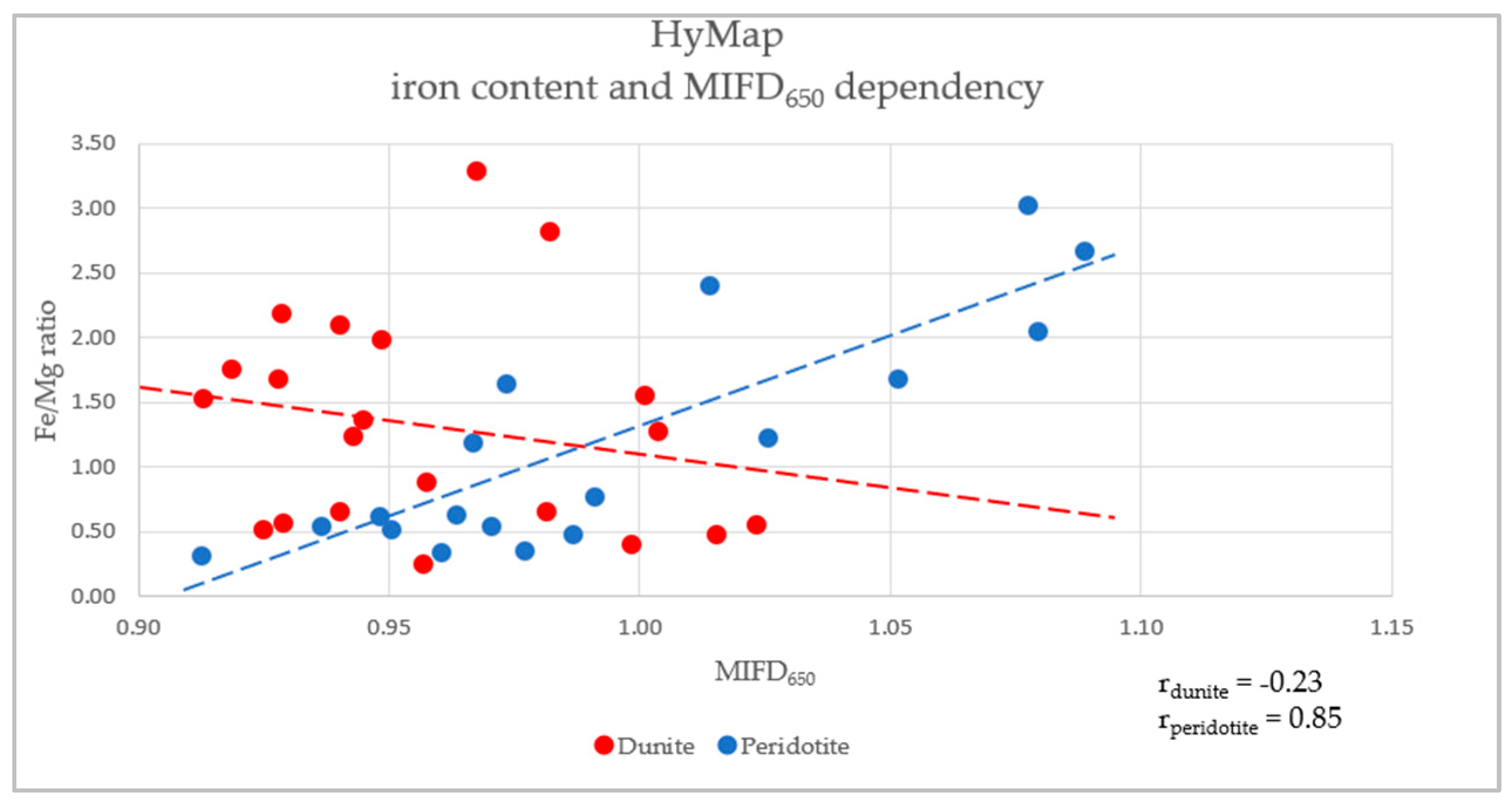
6.1. Fe/Mg Ratio and Modified Iron Feature Depth Index

Result 1—laboratory scale: The first preliminary result presents the Fe/Mg ratio plotted against the estimated sum of ferrous (MIFD650) and ferric (MIFD1000) modified iron feature depths for dunites (red) and peridotites (blue) (Figure 9).
The Fe/Mg content ratio was calculated on the basis of the LIBS measurements on hand specimens to display the dependency of the iron content on its absorption feature depths. The absorption features were extracted from the hand specimens measured in the laboratory in the simulated HyMap resolution (coarser spatial and spectral resolution of spectra). Figure 9 shows an overall linear trend indicating that the absorption feature depth tends to increase with increasing Fe-content or decreasing Mg-content for dunites and peridotites.
Result 2—airborne scale: Analogously, ferrous and ferric MIFDs were calculated for airborne HyMap scenes of the ultramafic complex. The Fe/Mg ratio values from rock samples were plotted against the ferric MIFD650 (Figure 10) and ferrous MIFD1000 (Figure 11) from HyMap data. Both figures show a robust, increasing linear trend for peridotite with a large correlation coefficient of 0.85 and 0.68) and a more vague decreasing linear trend for dunite (with lower correlation coefficients of −0.23 and 0.14).
The dunite body in the eastern part of the ultramafic complex shows a high abundance of large MIFD1000 values (dark red color), whereby MIFD650 values are lower abundant (light green color) in this area compared to its surroundings (Figure 12).
Fe3+ is the product of Fe2+ oxidation, forming secondary iron oxides/hydroxides on weathered rock surfaces. The generally high values for Fe3+ at 650 nm are partly associated with the oversaturation of the absorption band by the contribution of vegetation and lichen that partially covers the exposed rock surfaces in the study area. The combination of low MIFD650 and high MIFD1000 of the eastern dunite block compared to the remaining part of the ultramafic complex suggests that this area is less affected by alteration.

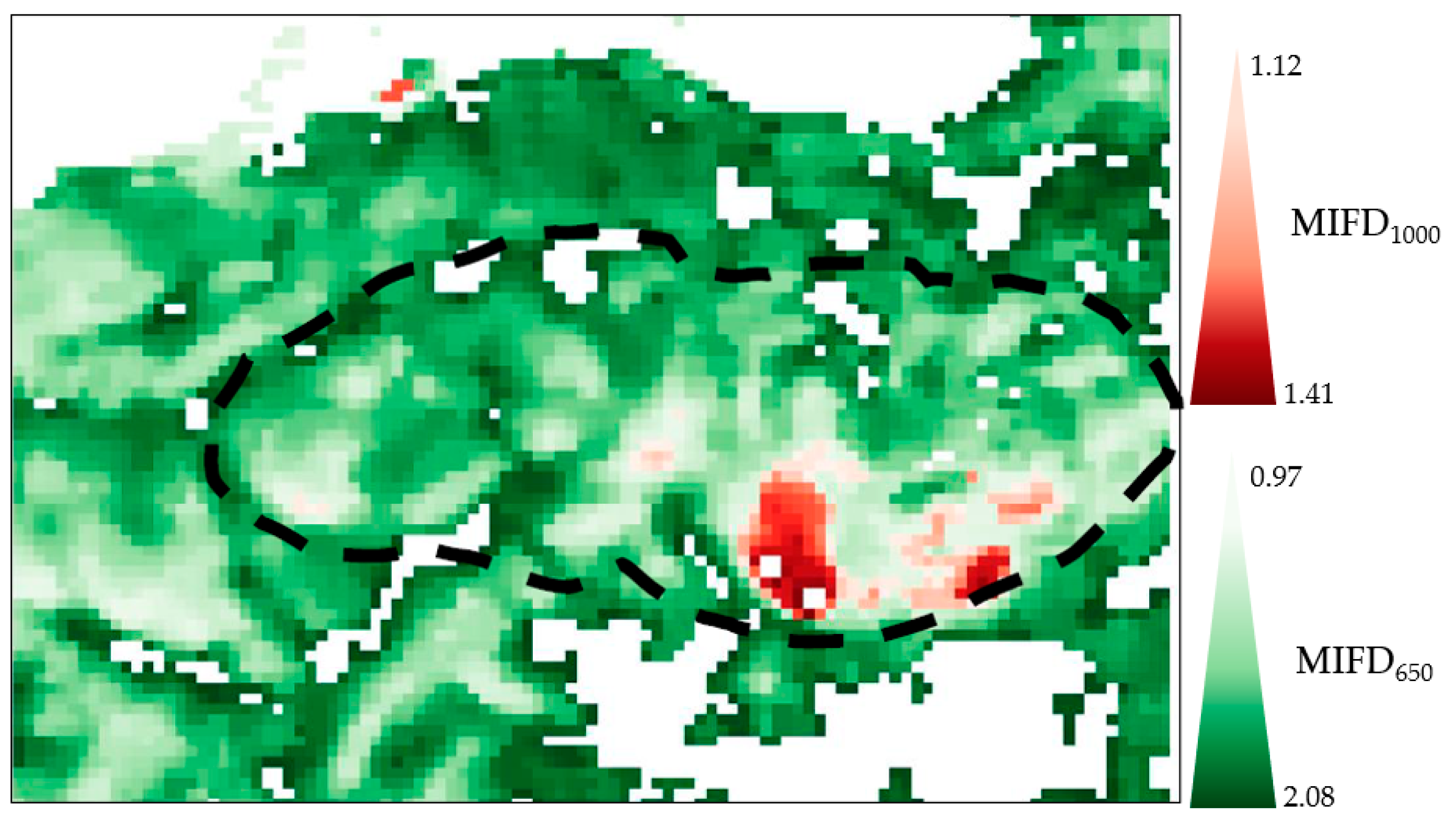
6.2. Integration of Hyperspectral and Magnetic Airborne Data

Result 3—airborne scale: The relationship between the residual magnetic anomaly data, ferrous MIFD1000, and ferric MIFD650 were analyzed by the forward modeling and inversion results approach. The predicted pseudo-magnetic responses from the Fe ratio (MIFD650/MIFD1000) (Figure 13B) are plotted against the high pass filtered residual magnetic anomaly data (Figure 13C) for the modeling approach in Figure 13A. The lithological information in Figura 13A is extracted from a geological map prepared by the company 21st North (Figure 1B).

7. Discussion

This study introduced a novel and robust approach for the geological characterization of an ultramafic complex with elevated magnetic properties based on integrating optical and magnetics datasets. This was achieved by establishing relationships between the residual magnetic anomaly data, ferric/ferrous ratios built from iron absorption feature indices, and lithological information (Figure 13). Primary lithologies in the complex are classified into three lithological groups (dunites, peridotites, and pyroxenites) that can be clearly distinguished based on how magnetic responses and susceptibility estimates correlate with iron absorption features from airborne-based hyperspectral data.
Magnetization depends on the primary magnetite’s rock composition and oxidation state [47]. As expected, areas dominated by peridotite are associated with the highest magnetization compared to areas dominated by dunite and pyroxenite. Lower magnetization values for dunites could indicate that the minerals in dunite are less ferruginous than in peridotites, thus containing more Mg.
Furthermore, the iron in dunite is also associated with chromite, which is not influenced by serpentinization and prevents the iron from being released [47]. Chromite has ferromagnetic properties [4], but the magnetization is lower than in magnetite.
Olivine weathers very quickly at and close to the surface and may form paramagnetic hematite that contains only ferric iron [67]. Ferric iron is stable under atmospheric conditions; therefore, the magnetization is lower for strongly weathered than for fresh rocks. In the plot, pyroxenites are weakly magnetized even at a high ferric/ferrous ratio. However, the magnetization increases slightly with increasing ferric iron content.
Considering the relationships in Figure 13, it becomes clear that it is partly difficult to distinguish dunite, peridotite, and pyroxenite-dominated rocks from magnetic data only. Similarly, it is impossible to distinguish pyroxenite and peridotite-dominated rocks only from hyperspectral iron ratios. However, separated clusters for the three lithologies can be observed by the combinations of both data types indicating that lacking diagnostic characteristics in one of the methods are provided by the other method.
The results highlight the benefit of the newly developed approach of combining the MIFD and residual magnetic anomaly data to both (1) detect which lithology is dominated by ferromagnetic magnetite found disseminated as an accessory mineral and (2) estimate how the oxidation state is related to the lithologies at the same time. Our results show that the correlation between residual magnetic anomaly, iron absorption features, and lithology (HSM integration) can be found in proxies. Furthermore, resolution enhancement of the residual magnetic anomaly data helps to unravel nondominant anomalies.
HS data acquired under laboratory settings provide detailed spectral information about the lithological units and rock types in the complex. Against that, a slight change in the illumination or the measuring angle and spectrometer-dependent measurement errors can bias the laboratory results [68,69]. Furthermore, reflectance spectra of an object acquired with different sensors may differ. A reliable mineral classification of HS data in the laboratory should rule out these error sources by applying a consistent spectral library of pure minerals measured using the same instrument utilized for sample analysis [70,71]. One step that needs to be followed before interpreting HS images consisting of two sensors with different spectral ranges (VNIR, SWIR) is the leveling adjustment. Due to this jump effect at 1000 nm, the result of combined VNIR and SWIR detectors can alternate the spectrum [57]. No detector jump is known in the case of HyMap, although the 650 nm absorption band is positioned close to the end of the spectral range, oversaturating the 650 nm absorption feature. Moreover, the 1000 nm band is more pronounced than the 650 nm band in almost all extracted spectra. The reason could be the spectral width of the absorption band close to 1000 nm that can be superimposed by the flanks of water vapor absorption features at 940 and 1130 nm.
It must be noted that the current approaches to combining airborne magnetic and hyperspectral data have several limitations. The magnetic forward modeling and inversion approaches assume that the magnetization only consists of an induced magnetization component (susceptibility) but not of a remanence component. In addition, the resolution of the magnetic method is limited such that the pixel values obtained from the magnetic modeling and inversion approaches have some inaccuracies and, hence, details in the cross-plots are not entirely correct. Another limitation is that a lichen spectrum has an absorption band close to 600 nm and could change the ferric iron absorption feature; moreover, lichen grows on specific lithologies such as peridotites, where the lichen can deteriorate spectral signature in the 400–2000 nm spectral region. In addition, the spectral signatures of ferrous (1000 nm) and ferric (650 nm) iron are distinctive due to the limited lichen cover in this range. Another iron absorption feature at 880 nm has been neglected in the analysis due to the high lichen presence in this spectral range. Therefore, an optimal weighting of the iron features and lichen presence is critical [12].
At multiple scales, e.g., laboratory, airborne-based, satellite-based, and spectral, information may not always be comparable [72]. Our results show that, regardless of scale, both laboratory and airborne-based iron absorption features are stable, making the HSM integration and validation of the results more accessible and feasible.

8. Conclusions and Outlook

This study proposed a novel method to integrate optical remotely sensed and aeromagnetic data using forward modeling and inversion approaches. This study is the first step in the geological analysis of ultramafic complexes based on multidisciplinary research with a strong focus on non-invasive mapping and remote sensing methods. This approach can help to improve the knowledge about the study site’s regional lithology and distribution of rocks and minerals by combining the partly complementary information from hyperspectral image products (Fe iron ratios) and magnetic properties. It is a promising way to analyze a prospect area with high iron-bearing mineral potential and can be considered as a starting point to integrate both data types by performing a more advanced hyperspectral constrained magnetic inversion. Our study on the ultramafic complex demonstrates that detailed airborne HSM-integration results can enhance our understanding of the geological origins of magnetic anomalies. It appears to be particularly useful to thoroughly characterize the distribution of Fe minerals, e.g., for iron-oxide and sulfide deposits.
Such a deposit must retain magnetic properties induced by the presence of both ferrous and ferric iron in minerals. We have shown that the HSM integration can be utilized based on chemical and physical rock properties presenting that the absorption feature depths of ferrous and ferric iron rise with the increasing ferrous and ferric iron amount in the analyzed dataset. The main benefit of the HSM integration is a significantly higher spatial resolution of the hybrid model and, thus, a better exploration possibility.
In our integration of imaging spectroscopy and aeromagnetics at an airborne scale, we used only the near-surface information in the forward modeling and inversion approaches. However, more research is needed to integrate hyperspectral imaging information into magnetic modeling or inversion approaches that consider models of both the near surface and at larger depths and are suited for complete geological characterization. Moreover, it is essential to find proper solutions to incorporate hyperspectral information as meaningful constraints in magnetic inversions. Such constrained inversions will improve the resolution of the magnetic models at shallow depths, making results from cross-plot more reliable and precise.
As a result, several theoretical assumptions and practical considerations should be considered before and while applying this approach:
  • We suggest collecting samples of the whole investigation area, including information about the sample’s orientation in the ground, to analyze the laboratory’s susceptibility and remanent magnetization. The rock samples should be geochemically analyzed, focusing on whole-rock analysis and titration to determine the rock’s ferric and ferrous iron content;
  • Since the magnetic properties can only be regionally correlated with the lithology, more research in a different climate and diverse iron-bearing deposits considering new parameters should prove our approach’s robustness.
Accordingly, a precise correlation of magnetic and HS properties is only possible if a proper estimate of the magnetization along the surface is determined using a modeling inversion technique. We can imagine that a magnetic inversion approach constrained by HS surface information is a possible strategy that can solve such problems in the future and better link the lithology at the surface obtained from hyperspectral with the magnetic anomalies determined in the (shallower) subsurface.

Author Contributions

Conceptualization, A.K., S.S., B.H.H. and C.R.; methodology, A.K., B.H.H., S.S., N.K., C.R.; software, A.K., C.R., C.M.; validation, B.H.H., C.R., N.K.; formal analysis, A.K., S.S., B.H.H., C.M.; investigation, A.K., N.K., S.S.; resources, S.S., C.R.; data curation, A.K.; writing—original draft preparation, A.K., B.H.H.; writing—review and editing, B.H.H., S.S., I.B.; visualization, A.K., B.H.H.; supervision, S.S., C.R., U.A., I.B. All authors have read and agreed to the published version of the manuscript.

Funding

The research was funded by the EnMAP scientific preparation program under the Space Agency at DLR with resources from the German Federal Ministry of Economic Affairs and Climate Action, grant number 50EE1529.

Data Availability Statement

Not applicable.

Acknowledgments

This work was carried out in collaboration with the University of Potsdam, the German Research Centre for Geosciences (GFZ), and the Geological Survey of Denmark and Greenland (GEUS). GEUS granted access to HyMap data. The authors would like to thank the 21st North company for supporting and sharing samples. Further, we thank Melanie Lorenz and Antje Musiol from the University of Potsdam for sample preparation and geochemical analysis. The authors also acknowledge Bjørn-Eirik Roald for proofreading the article.

Conflicts of Interest

The authors declare no conflict of interest.

References

  1. Mielke, C.; Muedi, T.; Papenfuss, A.; Boesche, N.K.; Rogass, C.; Gauert, C.D.K.; Altenberger, U.; Wit, M.J.D. Multi- and hyperspectral spaceborne remote sensing of the Aggeneys base metal sulphide mineral deposit sites in the Lower Orange River region, South Africa. S. Afr. J. Geol. 2016, 119, 63–76. [Google Scholar] [CrossRef]
  2. Jackisch, R.; Madriz, Y.; Zimmermann, R.; Pirrtijärvi, M.; Heincke, B.H.; Salmirinne, H.; Kujasalo, J.-P.; Andreani, L.; Andreani, R. Drone-Borne Hyperspectral and Magnetic Data Integration: Otanmäki Fe-Ti-V Deposit in Finland. Remote Sens. 2019, 11, 2084. [Google Scholar] [CrossRef]
  3. Dentith, M.; Mudge, S.T. Geophysics for the Mineral Exploration Geoscientist; Cambridge University Press: Cambridge, UK, 2014. [Google Scholar]
  4. Clark, D.A. Magnetic petrophysics and magnetic petrology: Aids to geological interpretation of magnetic surveys. J. Aust. Geol. Geophys. 1997, 17, 83–104. [Google Scholar]
  5. Hunt, C.P.; Moskowitz, B.M.; Banerjee, S.K. Magnetic properties of rocks and minerals. In American Geophysical Union; Geological Society of America: Boulder, CO, USA, 1995. [Google Scholar]
  6. Till, J.L.; Nowaczyk, N. Authigenic magnetite formation from goethite and hematite and chemical remanent magnetization acquisition. Geophys. J. Int. 2018, 213, 1818–1831. [Google Scholar] [CrossRef]
  7. Dekkers, M. Magnetic properties of natural goethite-III. Magnetic behaviour and properties of minerals originating from goethite dehydration during thermal demagnetization. Geophys. J. Int. 1990, 103, 233–250. [Google Scholar] [CrossRef]
  8. Oëzdemir, O.; Dunlop, D.J. Intermediate magnetite formation during dehydration of goethite. Earth Planet. Sci. Lett. 2000, 177, 59–67. [Google Scholar] [CrossRef]
  9. Hanesch, M.; Stanjek, H.; Petersen, N. Thermomagnetic measurements of soil iron minerals: The role of organic carbon. Geophys. J. Int. 2006, 165, 53–61. [Google Scholar] [CrossRef]
  10. Ager, C.M.; Milton, N.J.G. Spectral reflectance of lichens and their effects on the reflectance of rock substrates. Geophysica 1987, 52, 898–906. [Google Scholar] [CrossRef]
  11. Salehi, S.; Thaarup, S.M. Mineral mapping by hyperspectral remote sensing in West Greenland using airborne, ship-based and terrestrial platforms. Geol. Surv. Den. Greenl. 2017, 41, 47–50. [Google Scholar] [CrossRef]
  12. Salehi, S.; Mielke, C.; Rogass, C. Mapping ultramafic complexes using airborne imaging spectroscopy and spaceborne data in Arctic regions with abundant lichen cover, a case study from the Niaqornarssuit complex in South West Greenland. Eur. J. Remote Sens. 2020, 53, 156–175. [Google Scholar] [CrossRef]
  13. Rasti, B.; Hong, D.; Hang, R.; Ghamisi, P.; Kang, X.; Chanussot, J.; Benediktsson, J.A. Feature Extraction for Hyperspectral Imagery: The Evolution from Shallow to Deep (Overview and Toolbox). IEEE Geosci. Remote Sens. Lett. 2020, 8, 60–88. [Google Scholar] [CrossRef]
  14. Kopackova, V.; Koucka, L. Integration of absorption feature information from visible to longwave infrared spectral ranges for mineral mapping. Remote Sens. 2017, 9, 1006. [Google Scholar] [CrossRef]
  15. Kruse, F. Integrated visible and near-infrared, shortwave infrared, and longwave infrared full-range hyperspectral data analysis for geologic mapping. J. Appl. Remote Sens. 2015, 9, 096005. [Google Scholar] [CrossRef]
  16. McDowell, M.L.; Kruse, F. Enhanced compositional mapping through integrated full-range spectral analysis. Remote Sens. 2016, 8, 757. [Google Scholar] [CrossRef]
  17. Notesco, G.; Ogen, Y.; Ben-Dor, E. Integration of hyperspectral shortwave and longwave infrared remote-sensing data for mineral mapping of Makhtesh Ramon in Israel. Remote Sens. 2016, 8, 318. [Google Scholar] [CrossRef]
  18. Kuras, A.; Brell, M.; Rizzi, J.; Burud, I. Hyperspectral and Lidar Data Applied to the Urban Land Cover Machine Learning and Neural-Network-Based Classification: A Review. Remote Sens. 2021, 13, 3993. [Google Scholar] [CrossRef]
  19. Buckley, S.J.; Kurz, T.H.; Howell, J.A.; Schneider, D.J.C. Terrestrial lidar and hyperspectral data fusion products for geological outcrop analysis. Comput. Geosci. 2013, 54, 249–258. [Google Scholar] [CrossRef]
  20. Kirsch, M.; Lorenz, S.; Zimmermann, R.; Tusa, L.; Möckel, R.; Hödl, P.; Booysen, R.; Khodadadzadeh, M.; Gloaguen, R. Integration of Terrestrial and Drone-Borne Hyperspectral and Photogrammetric Sensing Methods for Exploration Mapping and Mining Monitoring. Remote Sens. 2018, 10, 1366. [Google Scholar] [CrossRef]
  21. Kirsch, M.; Lorenz, S.; Zimmermann, R.; Andreani, L.; Tusa, L.; Pospiech, S.; Jackisch, R.; Khodadadzadeh, M.; Ghamisi, P.; Unger, G.; et al. Hyperspectral outcrop models for paleoseismic studies. Photogramm. Rec. 2019, 34, 385–407. [Google Scholar] [CrossRef]
  22. Bedini, E.; Rasmussen, T.M. Use of airborne hyperspectral and gamma-ray spectroscopy data for mineral exploration at the Sarfartoq carbonatite complex, southern West Greenland. Geosci. J. 2018, 22, 641–651. [Google Scholar] [CrossRef]
  23. Jackisch, R.; Lorenz, S.; Kirsch, M.; Zimmermann, R.; Tusa, L.; Pirttijärvi, M.; Saartenoja, A.; Ugalde, H.; Madriz, Y.; Savolainen, M.; et al. Integrated Geological and Geophysical Mapping of a Carbonatite-Hosting Outcrop in Siilinjärvi, Finland, Using Unmanned Aerial Systems. Remote Sens. 2020, 12, 2998. [Google Scholar] [CrossRef]
  24. Bedini, E. Mapping lithology of the Sarfartoq carbonatite complex, southern West Greenland, using HyMap imaging spectrometer data. Remote Sens. Environ. 2009, 113, 1208–1219. [Google Scholar] [CrossRef]
  25. Bedini, E. Mineral mapping in the Kap Simpson complex, central East Greenland, using HyMap and ASTER remote sensing data. Int. J. Remote Sens. 2012, 33, 939–961. [Google Scholar] [CrossRef]
  26. Budkewitsch, P.; Staenz, K.; Neville, R.A.; Sangster, D. Spectral signatures of carbonate rocks surrounding the Nanisivik MVT Zn-Pb mine and implications of hyperspectral imaging for exploration in Arctic environments. In Proceedings of the Ore Deposit Workshop: New Ideas for a New Millennium, Cranbrook, BC, Canada, 5–6 May 2000. [Google Scholar]
  27. Harris, J.R.; Rogge, D.; Hitchcock, R.; Ijewliw, O.; Wright, D. Mapping lithology in Canada’s Arctic: Application of hyperspectral data using the minimum noise fraction transformation and matched filtering. Can. J. Earth Sci. 2005, 42, 2173–2193. [Google Scholar] [CrossRef]
  28. Salehi, S.; Lorenz, S.; Sørensen, E.V.; Zimmermann, R.; Fensholt, R.; Heincke, B.H.; Gloaguen, R. Integration of vessel-based hyperspectral scanning and 3D-photogrammetry for mobile mapping of steep coastal cliffs in the arctic. Remote Sens. 2018, 10, 175. [Google Scholar] [CrossRef]
  29. Tukiainen, T.; Thorning, L. Detection of kimberlitic rocks in West Greenland using airborne hyperspectral data: The HyperGreen 2002 project. Greenl. Bull. Geol. Surv. Den. 2005, 7, 69–72. [Google Scholar] [CrossRef]
  30. Tukiainen, T.; Thomassen, B. Application of airborne hyperspectral data to mineral exploration in North-East Greenland. Greenl. Bull. Geol. Surv. Den. 2010, 20, 71–74. [Google Scholar] [CrossRef]
  31. Jackisch, R.; Heincke, B.H.; Zimmermann, R.; Sørensen, E.V.; Pirttijärvi, M.; Kirsch, M.; Salmirinne, H.; Lode, S.; Kuronen, U.; Gloaguen, R. Drone-based magnetic and multispectral surveys to develop a 3D model for mineral exploration at Qullissat, Disko Island, Greenland. Solid Earth 2022, 13, 793–825. [Google Scholar] [CrossRef]
  32. Miller, C.A.; Schaefer, L.N.; Kereszturi, G.; Fournier, D. Three-Dimensional Mapping of Mt. Ruapehu Volcano, New Zealand, From Aeromagnetic Data Inversion and Hyperspectral Imaging. J. Geophys. Res. Solid Earth 2020, 125, e2019JB018247. [Google Scholar] [CrossRef]
  33. Simard, R.L.; Bliss, I.; Vaillancourt, C. Geological Report on Exploration and Drill Programs 2013—Licenses 2010/17, 2013727 and 2013/28; NorthernShield Ressources Inc.: West Greenland, Denmark, 2014; p. 43. [Google Scholar]
  34. Geotech. Report on a Helicopter-Borne Versatile Time-Domain Electromagnetic (VTEMplus) and Horizontal Magnetic Gradiometer Geophysical Survey; Niaqomarssuit Block: Greenland, Denmark, 2012. [Google Scholar]
  35. Gool, J.A.M.V.; Connelly, J.N.; Marker, M.; Mengel, F.C. The Nagssugtoqidian Orogen of West Greenland: Tectonic evolution and regional correlations from a West Greenland perspective. NRC Res. Press Web. 2002, 39, 665–686. [Google Scholar]
  36. Gothenborg, J.; Keto, L. Report on the aerial reconnaissance between Sukkertoppen Ice Calot and Nordenskiölds Gletscher. In Archives of Geological Survey of Denmark and Greenland; GEUS Report File 20210; Kryolitselskabet Øresund A/S: Copenhagen, Denmark, 1977. [Google Scholar]
  37. Østergaard, C. 21st North—2010 Field Work Qaqortorsuaq (Ikertoq), 2011; p. 99.
  38. Downes, H. Ultramafic Rocks. In Encyclopedia of Geology, 2nd ed.; Alderton, D., Elias, S.A., Eds.; Academic Press: Cambridge, MA, USA, 2021; pp. 69–75. [Google Scholar]
  39. Streckeisen, A.L. Plutonic rocks, classification and nomenclature recommended by the IUGS subcommission on the systematics of igneous rocks. Geotimes 1973, 18, 26–30. [Google Scholar]
  40. Philpotts, A.R.; Ague, J.J. Principles of Igneous and Metamorphic Petrology, 3rd ed.; Cambridge University Press: Cambridge, MA, USA, 2022. [Google Scholar]
  41. Ben-Dor, E.; Irons, J.; Epema, G. Soil reflectance. In Remote Sensing for the Earth Sciences: Manual of Remote Sensing; Rencz, A., Ed.; John Wiley & Sons: New York, NY, USA, 1999; pp. 111–188. [Google Scholar]
  42. Lin, J.F.; Speziale, S.; Mao, Z.; Marquardt, H. Effects of the electronic spin transitions of iron in lower mantle minerals: Implications for deep mantle geophysics and geochemistry. Rev. Geophys. 2013, 51, 244–275. [Google Scholar] [CrossRef]
  43. Bigham, J.M.; Fitzpatrick, R.W.; Schulze, D.G. Iron Oxides. In Soil Mineralogy with Environmental Applications; Soil Science Society of America Book Series; Dixon, J.B., Schulze, D.G., Eds.; Wiley: Hoboken, NJ, USA, 2002. [Google Scholar]
  44. Syverson, D.D.; Tutolo, B.M.; Borrok, D.M.; Jr, W.E.S. Serpentinization of olivine at 300 °C and 500 bars: An experimental study examining the role of silica on the reaction path and oxidation state of iron. Chem. Geol. 2017, 475, 122–134. [Google Scholar] [CrossRef]
  45. Gupta, R.P. Remote Sensing Geology; Springer: Berlin/Heidelberg, Germany, 2003. [Google Scholar]
  46. Kokaly, R.F.; Clark, R.N.; Swayze, G.A.; Livo, K.E.; Hoefen, T.M.; Pearson, N.C.; Wise, R.A.; Benzel, W.M.; Lowers, H.A.; Driscoll, R.L.; et al. USGS Spectral Library Version 7; USGS: Riston, VA, USA, 2017. [Google Scholar]
  47. Saad, A.H. Magnetic properties of ultramafic rocks from Red Mountain, California. Geophysics 1969, 34, 974–987. [Google Scholar] [CrossRef]
  48. Oufi, O.; Cannat, M.; Horen, H. Magnetic properties of variably serpentinized abyssal peridotites. J. Geophys. Res. 2002, 107, EPM 3-1–EPM 3-19. [Google Scholar] [CrossRef]
  49. Bach, W.; Paulick, H.; Garrido, C.J.; Ildefonse, B.; Meurer, W.P.; Humphris, S.E. Unraveling the sequence of serpentinization reactions: Petrography, mineral chemistry, and petrophysics of serpentinites from MAR 15 °N (ODP Leg 209, Site 1274). Geophys. Res. Lett. 2006, 33, L13306. [Google Scholar] [CrossRef]
  50. Hong, G.; Till, J.L.; Greve, A.; Lee, S.M. New Rock Magnetic Analysis of Ultramafic Cores From the Oman Drilling Project and Its Implications for Alteration of Lower Crust and Upper Mantle. J. Geophys. Res. Solid Earth 2022, 127, e2022JB024379. [Google Scholar] [CrossRef]
  51. McCollom, T.M.; Klein, F.; Moskowitz, B.; Berquo, T.S.; Bach, W.; Templeton, A.S. Hydrogen generation and iron partitioning during experimental serpentinization of an olivine–pyroxene mixture. Geochim. Cosmochim. Acta 2020, 282, 55–75. [Google Scholar] [CrossRef]
  52. Maar, G.W.t.; McEnroe, S.A.; Church, N.S.; Larsen, R.B. Magnetic Mineralogy and Petrophysical Properties of Ultramafic Rocks: Consequences for Crustal Magnetism. Geochem. Geophys. Geosyst. 2019, 20, 1794–1817. [Google Scholar]
  53. Cocks, T.; Jenssen, R.; Stewart, A.; Wilson, I.; Shields, T. The HyMap airborne hyperspectral sensor: The system, calibration and performance. In Proceedings of the 1st EARSeL Workshop on Imaging Spectroscopy, Zurich, Switzerland, 6–8 October 1998. [Google Scholar]
  54. Kruse, F.A.; Boardman, J.W.; Lefkoff, A.B.; Young, J.M.; Kierein-Young, K.S.; Cocks, T.D.; Jenssen, R.; Cocks, P.A. HyMap: An Australian hyperspectral sensor solving global problems-results from USA HyMap data acquisitions. In Proceedings of the 10th Australasian Remote Sensing and Photogrammetry Conference, Adelaide, Australia, 25 August 2000; pp. 18–23. [Google Scholar]
  55. Richter, R. Atmospheric/Topographic Correction for Airborne Imagery; DLR—German Aerospace Center: Wessling, Germany, 2010. [Google Scholar]
  56. Miziolek, A. Laser-induced breakdown spectroscopy—An emerging chemical sensor technology for real-time field-portable, geochemical, mineralogical, and environmental applications. Appl. Geochem. 2006, 21, 730–747. [Google Scholar]
  57. Rogass, C.; Koerting, F.M.; Mielke, C.; Brell, M.; Boesche, N.K.; Bade, M.; Hohmann, C. Translational Imaging Spectroscopy for Proximal Sensing. Sensors 2017, 17, 1857. [Google Scholar] [CrossRef]
  58. Rogass, C.; Segl, K.; Mielke, C.; Fuchs, Y.; Kaufmann, H. Engeomap—A geological mapping tool applied to the enmap mission. EARSeL eProc. 2013, 12, 94–100. [Google Scholar]
  59. Stark, P.B.; Parker, R.L. Bounded-Variable Least-Squares: An Algorithm and Applications. Comput. Stat. 1995, 10, 129–141. [Google Scholar]
  60. Clark, R.N.; Swayze, G.A.; Wise, R.A.; Livo, K.E.; Hoefen, T.M.; Kokaly, R.F.; Sutley, S.J. USGS Digital Spectral Library splib06a; Data Series 231; US Geological Survey: Reston, VA, USA, 2007.
  61. Pearson, K. On lines and planes of closest fit to systems of points in space. Philos. Mag. Lett. 1901, 2, 559–572. [Google Scholar] [CrossRef]
  62. Mielke, C.; Boesche, N.K.; Rogass, C.; Kaufmann, H.; Gauert, C.; Wit, M.D. Spaceborne Mine Waste Mineralogy Monitoring in South Africa, Applications for Modern Push-Broom Missions: Hyperion/OLI and EnMAP/Sentinel-2. Remote Sens. 2014, 6, 6790–6816. [Google Scholar] [CrossRef]
  63. Li, Y.; Oldenburg, D.W. Rapid construction of equivalent sources using wavelets. Geophysics 2010, 75, L51–L59. [Google Scholar] [CrossRef]
  64. Dilixiati, Y.; Baykiev, E.; Ebbing, J. Spectral consistency of satellite and airborne data: Application of an equivalent dipole layer for combining satellite and aeromagnetic data sets. Geophysics 2022, 87, G71–G81. [Google Scholar] [CrossRef]
  65. Aster, R.C.; Borchers, B.; Thurber, C.H. Parameter Estimation and Inverse Problems; Elsevier Academic Press: Amsterdam, The Netherlands, 2005; p. 301. [Google Scholar]
  66. Menke, W. Geophysical Data Analysis Discrete Inverse Theory; Academic Press Limited: Amsterdam, The Netherlands, 1989; Volume 45. [Google Scholar]
  67. Lessovaia, S.N.; Goryachkin, S.; Polekhovskii, Y.S. Soil formation and weathering on ultramafic rocks in the mountainous tundra of the Rai-Iz Massif, Polar Urals. Eurasian Soil Sci. 2012, 45, 33–44. [Google Scholar] [CrossRef]
  68. Funatomi, T.; Ogawa, T.; Tanaka, K.; Kubo, H.; Caron, G.; Mouaddib, E.; Matsushita, Y.; Mukaigawa, Y. Eliminating temporal illumination variations in whisk-broom hyperspectral imaging. Int. J. Comput. Vis. 2022, 130, 1310–1324. [Google Scholar] [CrossRef]
  69. Uezato, T.; Yokoya, N.; He, W. Illumination Invariant Hyperspectral Image Unmixing Based on a Digital Surface Model. IEEE Trans. Image Process. 2020, 29, 3652–3664. [Google Scholar] [CrossRef] [PubMed]
  70. Cardoso-Fernandes, J.; Silva, J.; Dias, F.; Lima, A.; Teodoro, A.C.; Barres, O.; Cauzid, J.; Perrotta, M.; Roda-Robles, E.; Ribeiro, M.A. Tools for Remote Exploration: A Lithium (Li) Dedicated Spectral Library of the Fregeneda–Almendra Aplite–Pegmatite Field. Remote Sens. 2021, 6, 33. [Google Scholar] [CrossRef]
  71. Koerting, F.M.; Koellner, N.; Kuras, A.; Boesche, N.; Rogass, C.; Mielke, C.; Elger, K.; Altenberger, U. A solar optical hyperspectral library of rare-earth-bearing minerals, rare-earth oxide powders, copper-bearing minerals and Apliki mine surface samples. Earth Syst. Sci. Data 2021, 13, 923–942. [Google Scholar] [CrossRef]
  72. Hong, Y.; Chen, S.; Chen, Y.; Lindermann, M.; Mouazen, A.M.; Liu, Y.; Guo, L.; Yu, L.; Liu, Y.; Cheng, H.; et al. Comparing laboratory and airborne hyperspectral data for the estimation and mapping of topsoil organic carbon: Feature selection coupled with random forest. Soil Tillage Res. 2020, 199, 104589. [Google Scholar] [CrossRef]
Figure 1. (A) True color HyMap image of the Niaqornarssuit Complex and (B) generalized geological map (1:10,000) of the Niaqornarssuit Complex (modified from [37]) with 23 rock sample locations (green marks) collected by the mineral exploration company 21st North Exploration and geochemically analyzed by the University of Potsdam. The white (A) and black (B) dashed polygon lines outline the ultramafic complex with a highlighted intrusion.
Remotesensing 14 04877 g001
Figure 2. The Niaqornarssuit complex from the southwest. The dashed lines outline the complex of 2 × 1 km size [37].
Remotesensing 14 04877 g002
Figure 3. Laboratory examples of spectral signatures in the spectral range of 400 to 2500 nm of (A) peridotite (olivine 40–90%), (B) dunite (olivine > 90%), and (C) pyroxenite (olivine < 40%) of collected rock samples from the Niaqornarssuit Complex. The measurements were conducted on the weathered surfaces of the rock samples from the study site (Figure 1). Blue rectangles represent the spectral range of absorption features from ferrous (Fe2+) and ferric (Fe3+) iron.
Remotesensing 14 04877 g003
Figure 5. Total magnetic intensity map of the aeromagnetic survey. The black lines indicate the flight lines. The yellow rectangle outlines the area around a mafic intrusion considered in magnetic and hyperspectral data integration.
Remotesensing 14 04877 g005
Figure 6. Generalized process chain of the proposed data integration approach.
Remotesensing 14 04877 g006
Figure 7. Schematic illustration of the MIFD1000 parameter estimation on a spectrum example of a peridotite sample (analogous to MIFD650).
Remotesensing 14 04877 g007
Figure 8. (A) Residual magnetic anomaly map after high pass filtering with a cut-off of 3000 m. (B) Inversion results from an equivalent dipole layer modeling. The dipoles are arranged in a uniformly spaced grid along the surface topography and are located in the center of the HS pixels. The precise DEM derived from the airborne survey (C) is used as the topography estimate. Dashed lines outline the shape of the ultramafic complex.
Remotesensing 14 04877 g008
Figure 9. Fe/Mg ratio versus MIFD of summed ferrous and ferric iron absorption depths for dunites (red) and peridotites (blue) calculated for HyMap spectral resolution in the laboratory. r values represent the correlation coefficients for each lithology. Dashed lines show the fitted linear trendlines for each lithology with the corresponding color.
Remotesensing 14 04877 g009
Figure 10. In-situ Fe/Mg ratio of the validation points versus MIFD650 for HyMap data. Dashed lines show the fitted linear trendline for each lithology with the corresponding color. r values represent the correlation coefficient for each lithology.
Remotesensing 14 04877 g010
Figure 11. In-situ Fe/Mg ratio of the validation points versus MIFD1000 for HyMap data. Dashed lines show the fitted linear trendlines for each lithology with the corresponding color. r values represent the correlation coefficient for each lithology.
Remotesensing 14 04877 g011
Figure 12. Results of the MIFD650 and MIFD1000 calculation for the HyMap scene. The red and green colors represent MIFD1000 and the MIFD650 associated with ferrous and ferric iron, respectively. The black dashed line outlines the study area—the Niaqornarssuit Complex.
Remotesensing 14 04877 g012
Figure 13. (A) Correlation plot between the residual magnetic anomaly data (after IGRF removal and high-pass filtering) and the pseudo-magnetic responses calculated by forward of MIFD650/MIFD1000-ratios that are considered as “susceptibility” values at the surface. The lithologies located immediately underneath data point locations are color-coded: dunites (orange), peridotites (gray), and pyroxenites (yellow) (B,C) show the calculated pseudo-magnetic response of the MIFD650/MIFD1000-ratio and the residual magnetic anomaly map, respectively. The dashed lines sketch the shapes of mapped dunites (orange), peridotites (gray), and pyroxenites (yellow) lithological units.
Remotesensing 14 04877 g013
Table 1. Magnetic gradiometer properties [34].
Magnetic GradiometerHorizontally Separated
Mean Altitude [m]87
Average speed [km/h]80
Sampling interval [s]0.1
Sensitivity [nT]0.001
Traverse line spacing [m]100 and 200
Tie line spacing [m]2000
Table 2. Key characteristics of the HyMap hyperspectral sensor [53] and HySpex cameras (AS).
SensorHyMapHySpex
VNIR-1600SWIR-320-e
Sensor typehyperspectralhyperspectral
Altitude [m]2500
Settingairbornelaboratory
Wavelength [nm]450–8901950–2480400–10001000–2500
890–1350
1400–1800
Bandwidth [nm]15–1618–203.76.25
Spatial resolution 3–10 m24 µm53 µm
DetectorHyMap MK 1
512 pixels
Si CCD
1600 × 1200
HdCdTe
320 × 256
FOV across track [°]61.31714
Pixel FOV across track [mrad]2.00.180.75
Pixel FOV along track [mrad]2.50.360.75
Publisher’s Note: MDPI stays neutral with regard to jurisdictional claims in published maps and institutional affiliations.

