Hyperspectral Reconnaissance: Joint Characterization of the Spectral Mixture Residual Delineates Geologic Unit Boundaries in the White Mountains, CA

Abstract

We use a classic locale for geology education in the White Mountains, CA, to demonstrate a novel approach for using imaging spectroscopy (hyperspectral imaging) to generate base maps for the purpose of geologic mapping. The base maps produced in this fashion are complementary to, but distinct from, maps of mineral abundance. The approach synthesizes two concepts in imaging spectroscopy data analysis: the spectral mixture residual and joint characterization. First, the mixture residual uses a linear, generalizable, and physically based continuum removal model to mitigate the confounding effects of terrain and vegetation. Then, joint characterization distinguishes spectrally distinct geologic units by isolating residual, absorption-driven spectral features as nonlinear manifolds. Compared to most traditional classifiers, important strengths of this approach include physical basis, transparency, and near-uniqueness of result. Field validation confirms that this approach can identify regions of interest that contribute significant complementary information to PCA alone when attempting to accurately map spatial boundaries between lithologic units. For a geologist, this new type of base map can complement existing algorithms in exploiting the coming availability of global hyperspectral data for pre-field reconnaissance and geologic unit delineation.

1. Introduction

Geologic maps undergird fundamental understanding of Earth’s history, drive billions of dollars in economic activity, and inform risks to lives and livelihoods from natural hazards [1]. Given the broad importance of these maps, their generation and interpretation have been a core competency for geologists since the origin of the field [2]. Recognizing the need for both accuracy and precision, earth scientists throughout the generations have incorporated technological advances throughout all stages of the mapping process.

Remote sensing has provided many of these advances, especially for reconnaissance prior to costly and sometimes dangerous field campaigns. Shortly after the invention of flight, visual interpretation of aerial photography started to be used for such geologic reconnaissance (e.g., [3]). Topographic structure has been studied for decades using photogrammetry (e.g., [4]), significantly enhanced in recent years with the development of rigorous, automated computation [5,6] and laser scanning [7]. Information about surficial mineralogy and weathering severity has also been recognized as a useful contributor to the geologic mapping process since the launch of the Landsat program (e.g., [8]). Interest in satellite and airborne remote sensing continues today, and the subject plays a growing role in geologic education, research, and industrial applications.

Imaging spectroscopy (IS), also known as hyperspectral imaging, is an emerging technology that promises to significantly advance geologic remote sensing. NASA has specifically highlighted this technology in the form of the Surface Biology and Geology (SBG) designated observable, both in the most recent Decadal Survey [9], and in planning for a multisatellite Earth system observatory [10]. Precursor missions are in development (including the successful July 2022 launch of the Earth Mineral Dust Source Investigation, EMIT; [11]), as are complementary missions from commercial ventures and other space agencies, such as ESA’s PRISMA and CHIME [12,13], DLR’s DESIS and EnMAP [14,15], and JAXA’s HISUI [16]. Critically, open data access agreements and rigorous intercalibration efforts are also planned. The depth and breadth of these efforts suggest that the 2020s may be the decade in which long-term global repeat coverage of decameter imaging spectroscopy data finally becomes a reality.

Despite decades of studies led by the development and operation of NASA’s Airborne Visible Infrared Imaging Spectrometer (AVIRIS; e.g., [17,18], for excellent historical perspective, see [19]) and extended to early spaceborne [20,21] IS, applications have faced both geographic (for airborne) and sensor performance (for spaceborne) limitations. The observations promised by a new generation of satellite-based sensors is expected to yield a wealth of new information for field geologists globally. However, fully exploiting this information will require the geologic mapping community to contend with the serious computational and conceptual challenges inherent to imaging spectroscopy data, such as high dimensionality, band-to-band correlation, and spectral nonuniqueness [22,23,24,25].

Mineral identification and mapping have been a core focus of airborne and laboratory reflectance spectroscopy for 50 years [11,17,26,27,28,29,30,31,32]. One proven approach has been to comprehensively characterize the reflectance signatures of known minerals in laboratory conditions (e.g., by the USGS Spectroscopy Lab [33]), then to determine and map dominant surface minerals through comparisons of observed pixel spectra to this library of known signatures. This approach, best known through the popular Tetracorder algorithm [17], has been shown to consistently yield accurate and precise mineral maps even in challenging terrestrial and extraterrestrial landscapes (e.g., [17,34,35,36,37]).

Further, as recently reviewed by [38], a wide range of other algorithms have been developed for the use of imaging spectroscopy in lithological mapping, mineral exploration, and environmental geology. One popular set of tools is used for statistical endmember selection, including approaches such as the pixel purity index [39], N-finder [40], and vertex component analysis [41]. Another set is used for discrete image classification, including both traditional algorithms like maximum likelihood (e.g., [42]) and support vector machines [43], as well as more recent neural network-based approaches [44,45]. Such discrete classification approaches almost entirely operate using various statistical operators to partition the variance-based spectral feature space. A need thus still exists for a complementary approach which (1) does not require an a priori spectral library, (2) explicitly accommodates subpixel spatial mixing, and (3) isolates potentially lithologically informative low-variance absorption signals from potentially confounding high-variance continuum-driven land cover signals.

Here, we present a new approach for the application of imaging spectroscopy to geologic mapping. The approach is designed to complement the successes of mineral mapping algorithms, such as Tetracorder [17]. The foundational premise begins with the observation that, for some applications, rocks—assemblages of minerals—may be the primary unit of interest to the geologist (rather than, or in addition to, the individual minerals). From this premise, we designed a new characterization approach that seeks to directly identify regions of observed geologically relevant spectral similarity—i.e., potential map units—within a geographically defined study area.

As highlighted by [46,47,48,49] and recently summarized by [50], a special need exists for algorithms capable of harnessing the power of recent advances in machine learning, while retaining the key criteria of transparency, interpretability, and uniqueness of results. The approach introduced here works towards this need by leveraging the deep information content of spectroscopic data in a way that is specifically tailored to the needs of geologists. Conceptually, the approach can be considered as lying at the nexus of physically based linear models and statistically based nonlinear models. On the physical side, the spectral mixture residual (MR; [51]) offers a fast, scalable, and generalizable decomposition of high-variance spectral features in the mixed pixels that dominate decameter-resolution imagery. On the statistical side, the exploration of joint multiscale characterization (JC; [52], followed by [53,54]) offers a novel approach to the characterization and modeling of low-variance spectral features as statistically distinct nonlinear data manifolds. To date, these two approaches have been developed separately and for differing applications: MR has largely been framed in the context of vegetation and terrestrial ecology, and JC in the context of cryospheric, agricultural, and spatiotemporal applications. To our knowledge, this work presents the first investigation into the potential value of the union of the two approaches.

The algorithm works as follows: first, the initial application of the MR pretreats the image to isolate the signals of geologic interest from confounding contributions of vegetative cover and terrain effects. The subsequent application of JC then works across scales of variance to leverage spatially and/or spectrally coherent manifolds with (potentially) high geologic information, but low contributions to overall spectral variance.

Using archival AVIRIS-classic data from a previously mapped area of the White Mountains, CA (Figure 1), field investigation, and knowledge of regional geology, we demonstrate this example MR + JC methodology and ask the following questions:

(1)

To what extent can the imaging spectroscopy-based mixture residual provide a useful pre-field characterization of an area with highly diverse geology?

(2)

What information emerges from the synergy between the mixture residual and joint characterization? How does this differ from principal component (PC)-based characterization?

(3)

What is the conceptual difference between the information provided by this approach and the information that would be provided by existing approaches to mapping mineral presence and abundance (e.g., Tetracorder)?

(4)

In what ways can this new information be relevant for geologic mapping?

The remainder of the paper is organized as follows. First, we outline both the geologic and remote sensing data used for the analysis. Next, we provide a brief description of the IS processing methodology. We then provide a detailed demonstration of the results produced by each step in the methodology, demonstrating the outcome of the analysis both geographically (in map space) and statistically (in spectral feature space). Finally, we discuss results and summarize conclusions in the context of geology, geophysics, remote sensing, and machine learning.

2. Data

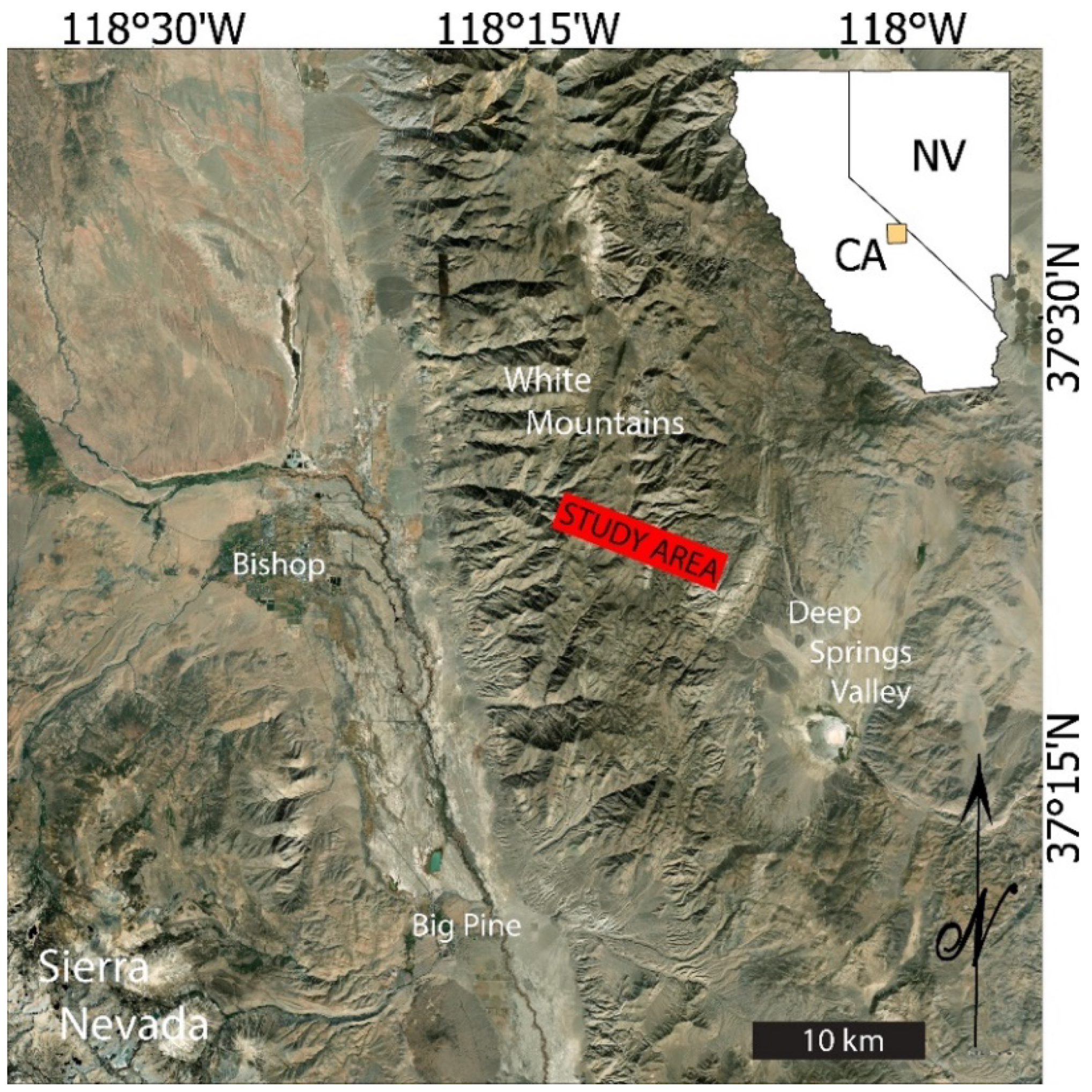
2.1. Study Site

2.1.1. Geology

Bedrock geology of the study area includes a diversity of lithologic units, including Precambrian to Cambrian metasedimentary rocks of the White-Inyo succession ([55]; citations therein), and the Late Cretaceous Birch Creek pluton that intrudes and deforms the older section [56]. The metasedimentary units primarily consist of either carbonate or mixed carbonate-siliciclastic lithologies, and include the Wyman Formation, Reed Dolomite, Deep Spring Formation, Campito Formation, Poleta Formation, Harkless Formation, and Emigrant Formation. The Cretaceous Birch Creek pluton consists of quartz monzonite and granodiorite and was emplaced circa 82 Ma [57]. The spatial distribution of bedrock units is documented in a published geologic map [58].

2.1.2. Site Selection

Several scientific reasons inform our decision to focus this work on this particular area of geologic interest at Schulman Grove, White Mountains, CA. Foremost is scientific popularity across a broad range of disciplines. Published geologic maps of this area have been available since at least the 1960′s [58], and in the intervening decades, a significant body of work has been developed utilizing the White Mountains as a natural laboratory [59,60,61]. While this includes important contributions to our understanding of lithospheric evolution [62], it also spans other areas of fundamental research of broad interest to the scientific community, e.g., dendrochronology [59,63] and animal physiology [64]. Additionally, the site is a classic locale for geoscience education. Over the last half of the 20th century, the White Mountains have hosted 1000s of student geologists developing their geologic mapping skills [65,66]. These reasons, together with the lithologic and geochemically distinct bedrock units and spatial heterogeneity, make this study site an excellent proving ground for this study. For field geologists who are not experts in imaging spectroscopy—the intended audience of this paper—the popularity of the site within the geologic education community suggests this location might provide valuable intuition that might be less well developed at the traditionally popular location for hyperspectral algorithm testing within the remote sensing community, Cuprite, NV [27,67,68,69,70].

2.2. Airborne Imaging Spectroscopy

Imaging spectroscopy data were collected by the Airborne Visible Infrared Imaging Spectrometer (AVIRIS-classic) on 17 September 2018. Level-2 surface reflectance data were downloaded free of charge from the Jet Propulsion Laboratory’s AVIRIS data portal at: https://aviris.jpl.nasa.gov/dataportal/ (accessed 3 Feburary 2022). All analysis was based on a single cloud-free flightline (f180917t01p00r06—HyspIRI_3_Line49—NASA Log # 182023). Flight azimuth was approximately NNE to SSW. The local time of collection was between 13:08 and 14:02. Pixel size was 13.5 m. ATREM-based atmospheric correction [71] was implemented before being downloaded from the web portal. Notably, ISOFIT [72] atmospheric correction was additionally run on Level-1 at-sensor radiance data. Analyses were repeated using these data, and comparable (though not identical) results were found. A detailed comparison of results on ATREM vs. ISOFIT corrections was beyond the scope of this study but presents an important avenue for future work. The analysis below proceeds using the ATREM-based reflectance data, which are currently most commonly available for direct download from the AVIRIS-classic web portal.

An exemplary 750 × 150 pixel spatial subset (Figure 2) was selected from the full 1205 × 46,354 pixel orthorectified AVIRIS flightline on the basis of geologic diversity using one author’s (FJS) knowledge of the area. Bands 1–5, 59–65, 104–120, 142–148, 154–179, and 220–224 were excluded (corresponding to wavelengths 365–404, 908–966, 1322–1482, 1701–1761, 1820–2046, and 2455–2496 nm) due to atmospheric contamination and/or visually apparent sensor artifacts. Bad lines were further masked by removing all pixels with any nonphysical (< 0 or > 1) reflectance value in any non-excluded band.

3. Methods

Analysis proceeded in three main stages:

• Linear spectral unmixing with retention of the spectrally explicit mixture residual.
• Joint characterization based on both linear and nonlinear dimensionality reduction.
• Geologic interpretation.

Methods for stages 1 and 2 are described briefly below. For more detailed methodological description of each stage, the reader is referred to the original literature introducing each of the MR and JC approaches, referenced below.

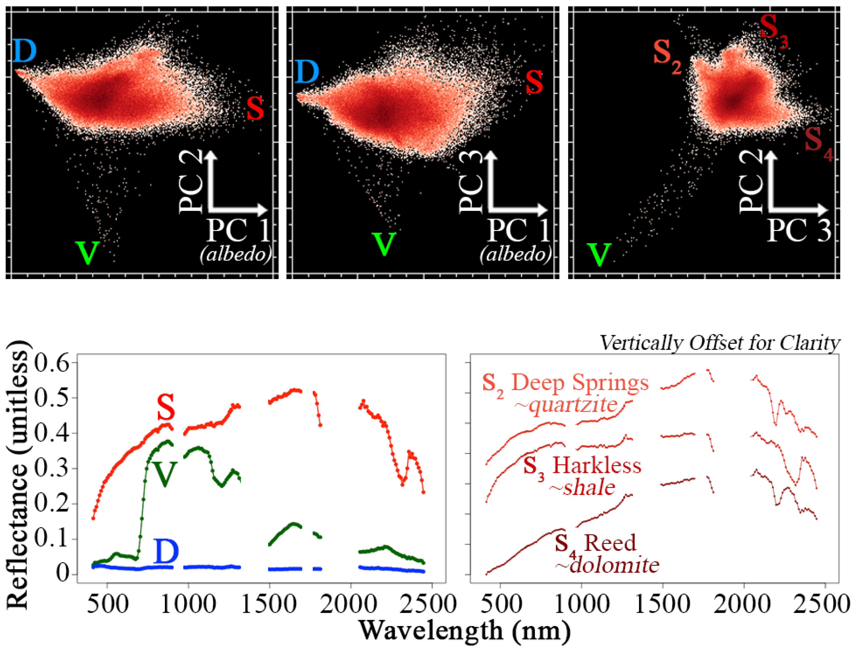
3.1. Linear Spectral Unmixing and Mixture Residual

First, the mixture residual procedure of [51] was implemented. Briefly, this consisted of:

• Manual selection of local spectral endmembers.
• Simultaneous estimation of the spectral endmember fraction and mixture residual spectrum (observed—modeled reflectance) for each pixel.

To select local endmembers, the spectral feature space was computed using the covariance-based principal component (PC) transform. Algebraically,

D = U Σ V

(1)

where D is the (geographically unwrapped) n × m matrix of pixel reflectance spectra, U is the n × n matrix of spatial PCs, Σ is the n × m (diagonal) matrix of singular values, and V is the m × m matrix of (uncorrelated) spectral eigenvectors. The conceptual effect of the PC transform can be understood as a linear tool to distill image variance. In the reflectance image, this variance is spread unevenly across all channels of the image. In the PC image, variance is distributed preferentially into weighted contributions of a small number of uncorrelated spectral patterns.

Endmember selection was performed manually through interrogation of the low-order PC-based spectral feature space computed from all pixels in both subsets. As noted by [73], the various generative signals within the ground sampling distance of a single imaging spectroscopy pixel can be profitably considered to comprise elements of a convex set. Thus, the geometric relationships of pixel spectra within a high-dimensional spectral feature space imply algebraic structure which can be formulated in the mixing equations. Briefly, vertices in spectral feature space represent compositionally pure spectral endmembers which form a spectral mixing space. Straight edges connecting vertices represent binary linear mixing relations between these vertices, and pixels plotting interior to the space can be considered mixture of more than 2 endmembers (e.g., Figure 3), with a conceptual analog to a geologist’s barycentric plot (better known as a ternary diagram).

In order to demonstrate broad applicability and relevance to global applications, we selected generic substrate, vegetation, and dark (S, V, and D) endmembers. S, V, and D endmembers have been shown to well-characterize diverse global compilations of Landsat [74,75,76], MODIS [77], and Sentinel-2 [78] multispectral data, as well as regional compilations of AVIRIS-classic [79], and AVIRIS-ng [51,80] spectra. Conceptually, these endmembers were not selected on the basis of providing an optimal pixelwise spectral fit, as in multiple endmember spectral mixture analysis (MESMA; [81]). Rather, they were selected for global generality and computational efficiency. We also note that generalized global endmembers are likely to be developed from stable satellite sensors in the near future.

The implementation of the linear spectral mixture model and computation of the mixture residual spectrum is linear, invertible, and computationally efficient (<1 s to compute modeled, residual, and fraction images for this study area on a laptop computer with 32 GB RAM, 2GHz Quad-Core Intel Core i5 CPU, 1536 MB Intel Iris Plus Graphics GPU). The mixture residual code is fully open source and the computation of the residual spectrum itself can be performed in one line of Python code. Algebraically,

R = [1 − G(G^TG)⁻¹G^T]D

(2)

where D is the (geographically unwrapped) n × m matrix of pixel reflectance spectra, G is the m × p matrix of endmember reflectance spectra, and R is the (geographically unwrapped) n × m matrix of mixture residual pixel spectra.

The effect of Equation (2) is to compute an image which describes the spectrally explicit misfit of the mixture model at each pixel. Conceptually, this residual image encodes the wavelength-specific difference between each pixel’s observed reflectance spectrum and the reflectance that would have been observed if the linear mixture model were perfectly accurate.

We further note that the linear mixing model used in Step 1 does not fit important nonlinear mixing processes. Instead, it computes a first-order linear fit, and partitions any signals not modeled by simple linear mixing into the spectrally explicit residual. To the extent that nonlinear mixing processes result in a misfit from a simple linear model, this information is explicitly leveraged in the subsequent joint characterization step. We also emphasize that, in this context, the residual spectra are not intended for direct physical interpretation. Rather, they are used statistically as quantitative information about processes (nonlinear or otherwise) that are not well-fit by a simple linear S, V, and D mixture.

For more background and details about the mixture residual, see [51]; for inspirational early studies, see [82,83].

3.2. Joint Characterization

Next, the joint characterization (JC) methodology introduced by [52] and extended by [53,54,84] was applied to the mixture of residual images.

Conceptually, JC seeks to characterize spectral information across scales of variance. This is achieved by contrasting the characterization of statistically global patterns of image variance with the characterization of statistically local patterns of image variance. In theory, the combination of global and local approaches should provide more information about the land surface than either approach alone.

In the context of imaging spectroscopy, the “continuum-plus-absorption” cognitive model has been used for decades as a useful analytical framework (e.g., [30,32,85]). Briefly, this approach consists of decomposing the spectral signal quantified by decameter-scale reflectance observations into two constituent components. One component, the spectral continuum, varies mainly in overall amplitude and curvature. The other component, specific absorption features, can be characterized using measures, such as precise center wavelength, depth, and asymmetry—potentially in a diagnostic fashion associated with a particular composition (e.g., individual mineral, or mineral association).

Joint characterization under this conceptual regime can be considered a mechanism for using an appropriately matched analytic tool for each aspect of the measurement. Several properties of the spectral continuum — high amplitude variability, correlation across many spectral bands, and limited observed variability in spectral shape across landscapes—are well-suited for variance-based tools, such as PCA and spectral mixture analysis (i.e., the methods of Section 3.1). In contrast, several properties of absorption features—low overall amplitude, significant variability in center wavelength, and high observed variability across landscapes—are less well-suited for mathematical approaches that rely on overall spectral variance alone, and are potentially better suited for alternative characterization approaches, such as manifold learning.

Here, we implemented an abbreviated variation of the full JC methodology. Following [53], we used t-distributed stochastic neighbor embedding (t-SNE; [86]) to isolate data manifolds and stabilize the t-SNE output using a Monte Carlo approach. Briefly, t-SNE is a nonlinear dimensionality reduction algorithm designed to find clustering relationships within high-dimensional data. This is achieved by minimizing the Kullback–Leibler divergence between pairwise statistical similarity among data points in high-dimensional space (here, the full 200+ band AVIRIS pixel spectra) and pairwise statistical similarity among data points in a low-dimensional embedding (here, a 2D representation of these spectra).

A notable limitation of t-SNE, along with many other manifold learning algorithms, is its dependence on initial seeding and hyperparameter choice, in particular the perplexity hyperparameter. Here, we stabilize the characterization by computing several t-SNE realizations and applying a PC transformation to the stack of t-SNE outputs (following [53]). The result, deemed PC[t-SNE(MR)], identifies pixel clusters which are consistent among iterations. We used 10 iterations with default scikit-learn perplexity and learning rate hyperparameter values. In theory, this approach should retain the sensitivity to low-variance features provided by t-SNE. It should also improve interpretability and stability by reinforcing separation between sets of pixels which are repeatedly identified as clusters in multiple t-SNE realizations, and mitigate the problem of nonuniqueness, which is inherent to single t-SNE realizations. We note that this algorithm is entirely open source and computationally feasible using commercially available hardware (for this analysis, all t-SNE runs were computed in <12 h on a laptop computer with a 32 GB RAM, a 2GHz Quad-Core Intel Core i5 CPU, and a 1536 MB Intel Iris Plus Graphics GPU).

Once PC(t-SNE) is computed, we interactively analyze the PC(t-SNE) result. Clusters are determined manually by the user. While cluster delineation could, of course, be automated, current automation methods were found to produce less satisfactory results than manual delineation. Cluster labels are assigned by comparing the geographic location of pixel clusters to the geologic map, then confirmed with targeted field observations. Since the final cluster selection is manual, the number of unclassified pixels can be increased or decreased easily by contracting or expanding the clusters. We use ENVI software for this step of visualization and manual cluster selection, but note that open-source Python alternatives, such as Glue (https://docs.glueviz.org/en/stable/ accessed on 3 February 2022), could be used instead.

Finally, we note that the PC(t-SNE) approach is one realization of the general approach. While PC(t-SNE) is found to give useful results in this analysis, we note that manifold learning is currently a rapidly evolving field. Additional testing is underway, and it is possible that other algorithms, e.g., uniform manifold approximation and projection (UMAP) [87], may supplant PC(t-SNE) as a more useful practical implementation of the low-variance component of JC. However, while the details of the implementation are sure to evolve, this will not alter the fundamental idea proposed here: that both high-variance and low-variance features can each be explicitly characterized, and can each contribute important information to imaging spectroscopy for geologic mapping.

4. Results

4.1. Endmember Selection

The combined low-order spectral feature space was visually examined, and endmember spectra were selected. The variance-based low-order spectral feature space was found to be bounded by three dominant spectral signatures—substrate, vegetation, and dark. This result is in accordance with previous, more spatially extensive studies of imaging spectroscopy data [51,79] as well as global multispectral studies [74,75,76,77].

As expected for such a diverse study site, a single generic, spectrally convex substrate endmember is clearly unable to represent the full complexity of the geologic signatures in the area (e.g., S2–4 in Figure 3). Endmember S2 corresponds to the quartzite dominant Deep Springs Formation (d), Endmember S3 corresponds to the shale-rich Harkless Formation (Ꞓh), and Endmember S4 corresponds to the carbonate Reed Dolomite (r); (See Discussion for more detail). For this reason, we used a multipixel mean S spectrum in our initial mixture model. The goal of this step was primarily to model and remove the high variance and relatively uninformative spectral continuum (estimated with endmember fraction images). This allows subsequent analysis to focus specifically on the narrowband absorption signatures (which are not fit by the mixture model, but are retained in the mixture residual spectrum), which have lower overall spectral variance but higher geologic information content.

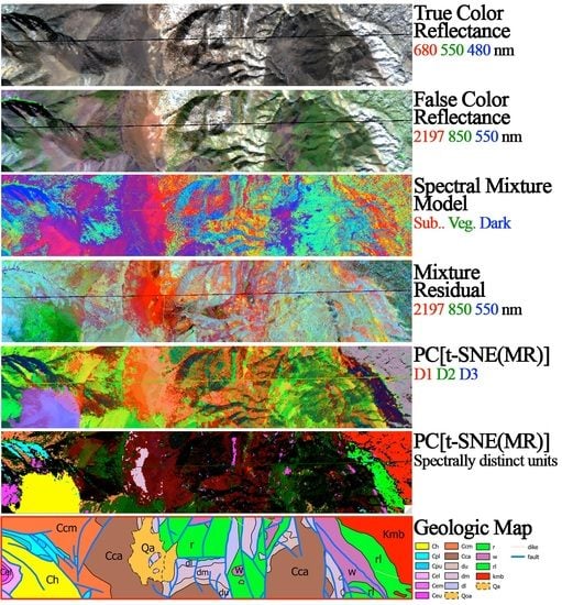
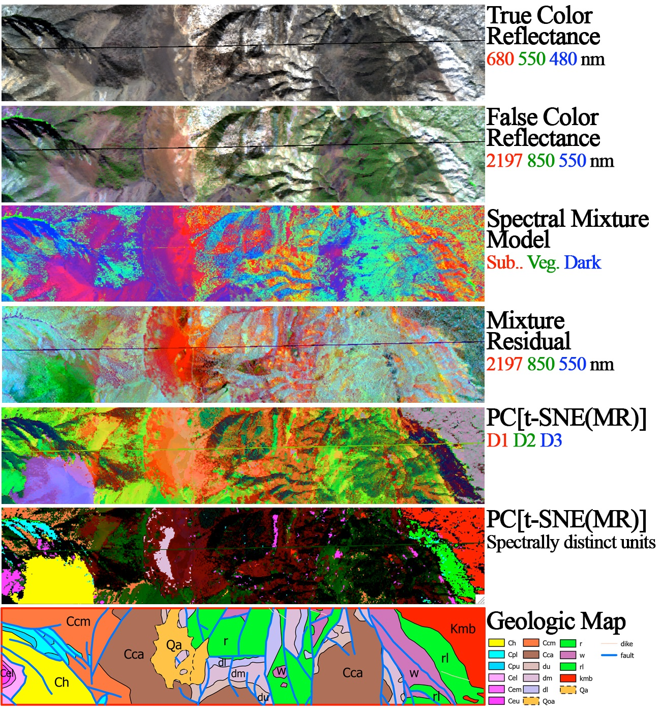
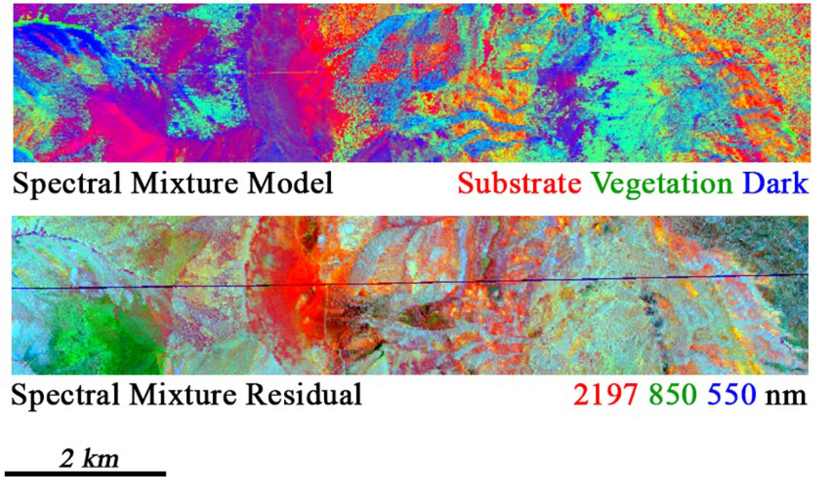
4.2. Mixture Model Performance

Despite the geologic complexity of the study area, over 99% of pixels are characterized by S and D fraction estimates within physical [0, 1] bounds (Figure 4). The V fraction estimates do include a nontrivial number (12%) of nonphysical negative pixel values, largely driven by the significant amount of observed variability in the concavity of the NIR spectral continuum in some geologic substrates. The root mean square mixture model misfits are < 5% for > 98% of the image pixels. However, despite this low amplitude, it is precisely the spectral signatures retained within this misfit which are shown to yield substantial geologic information in subsequent stages of the analysis.

The resulting spectral mixture fraction map (Figure 5, top) provides spatial approximations of photosynthetic vegetation cover and substrate exposures, as well as albedo and variations in illumination and topography. While useful from the perspective of land cover mapping, these spatial patterns are relatively uninteresting geologically. The converse is found for maps based on spectral mixture residuals, as presented below.

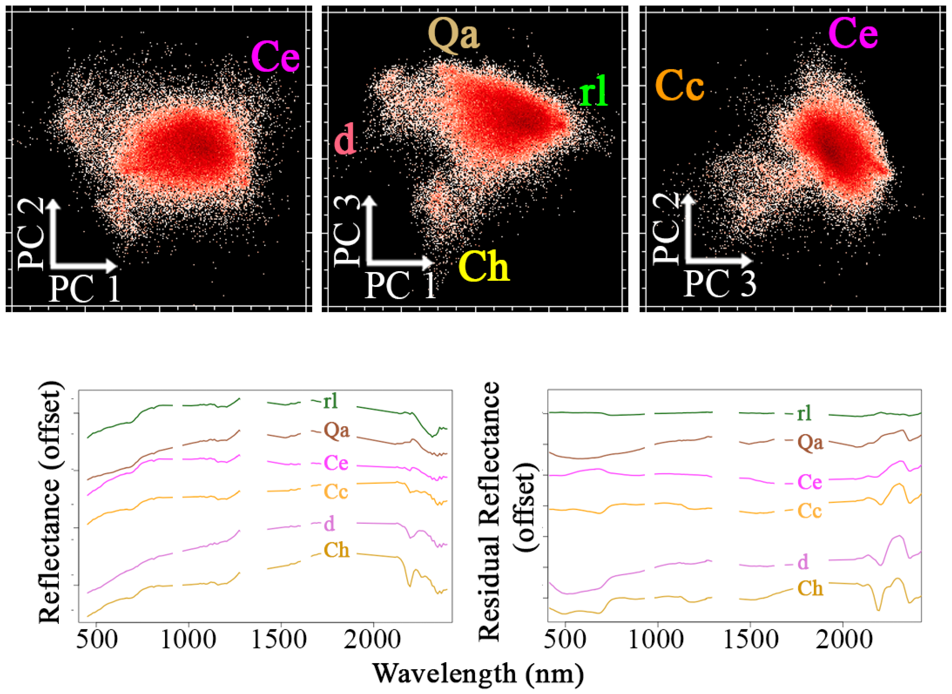
4.3. Mixture Residual

In contrast to the broad patterns associated with vegetation cover and topography found by the spectral mixture model, the wavelength-dependent spectral mixture residual (Figure 5, bottom) yields geologically interesting patterns which are found to correlate well with both differences among map units and compositional heterogeneity within map units. The richer information content of the mixture residual is visually apparent when the false color composite of Figure 5 is compared to the true color and false color composite images previously shown in Figure 2.

Low dimensional projections of the spectral feature space of the mixture residual image (Figure 6, top) suggest a truncated tetrahedral geometry. Surface reflectance spectra of mixture residual endmembers show similarity at VNIR wavelengths and divergence at SWIR wavelengths, while mixture residual spectra generally retain the narrow SWIR absorptions but also capture much more deviation at VNIR wavelengths (Figure 6, bottom). As stated above, we do not suggest that the signals in the mixture residual spectra necessarily possess direct physical, mineralogical, or optical meaning. Rather, we use these signals statistically, focusing on the information which might be provided by (potentially low variance) topological connectivity and clustering relations.

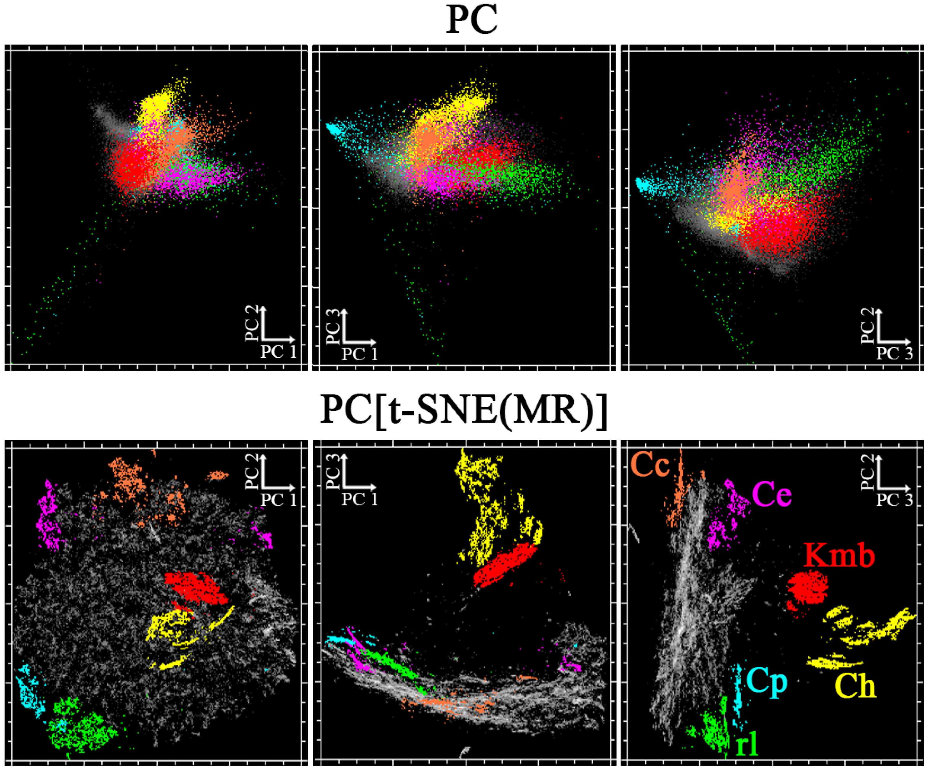
4.4. The PC[t-SNE(MR)] Spectral Feature Space

The multiscale variance structure of the data is then explored through the PC[t-SNE(MR)] feature space (Figure 7, bottom), compared to the PC feature space of the untransformed reflectance (Figure 7, top). The PC[t-SNE(MR)] spectral feature space clearly exhibits a more clustered topology, in many cases with readily identifiable boundaries among pixel clusters. Spectrally distinct rock units were isolated from pixel clusters in the PC[t-SNE(MR)] 3 vs. 2 projection and back-propagated to the other projections. Several regions of interest, which are ambiguous and indistinct in the PC space (top), are unambiguous and clearly distinct in the PC[t-SNE(MR)] space (bottom). The implications of this result for geologic mapping are profound.

Compared to each other, the PC-based spectral feature space clearly offers a more continuous projection, while the PC[t-SNE(MR)] spectral feature space visibly enhances class separability. Decision boundaries among geologic map units are ambiguous at best from the PC-based space, while regions of interest selected from the PC[t-SNE(MR)] space are visually clearer and statistically unambiguous (transformed divergence = 2.0 for all pairs shown).

In many cases, regions selected from the PC[t-SNE(MR)] feature space also frequently demonstrate both high-fidelity agreement with detailed geologic maps of the area and additional nuances that were not clearly identifiable in the geologic map alone. Specific geologic observations are briefly presented in the following subsection and further expanded in the discussion section.

4.5. Geology

It is clear from inspection that several pixel clusters identified from the mixture residual and joint characterization directly correlate to geologic map units from field-based observations (two lower frames on the left side of Figure 8). The three most clearly distinguished rock units that accurately locate the mapped bedrock contacts are (1) the Cretaceous Birch Creek pluton (red, map unit Kmb), (2) the lower member of the Precambrian Reed dolomite (green, map unit rl), and (3) the Cambrian Harkless Formation (yellow, map unit Ꞓh). Several of the other pixel clusters partially correspond to bedrock units and overlap the mapped bedrock contacts (e.g., cyan and orange), as does a significant part of the Quaternary surficial deposits (pale pink). A more detailed explanation of the distinctive characteristics of the three clusters most congruent with bedrock map units, as well as the specific geologic conditions of the partially overlapping clusters, is included in the discussion below.

5. Discussion

5.1. Remote Sensing

5.1.1. Conceptual Overview and Distinction from Mineral Mapping Algorithms

We emphasize that the approach presented here is not intended to be exclusive of established mineral mapping algorithms. Rather, we suggest that, in some cases, it may provide additional useful information—both quantitative and qualitative—which may complement mineral maps in conducting a comprehensive geologic characterization of a study area. We expect this information to be most useful as basemaps to use while planning fieldwork, but clearly, some information is likely to be additionally useful for post-field consideration and formulation of the final mapping product.

Expanding upon this, we suggest the approach presented here can be framed using (at least) the following four conceptual models:

• As imaging spectroscopy data with global coverage becomes available in the future, this tool can help translate that data into usable products for geologic reconnaissance.
• To the geophysical inverse theory community, the approach can be considered an attempt to formulate outcrop delineation from hyperspectral imagery as a “well-posed problem” through a two-step procedure which partitions high-variance from low-variance signals.

  ○

  High-variance signals are: (1) attributed to spatial land cover mixing, (2) considered continuous (albeit computationally discrete) parameters, and (3) estimated using a linear, invertible, and physically based inverse model.

  ○

  Low-variance signals are: (1) attributed to geologic drivers, such as mineralogy and chemical weathering, (2) considered categorical parameters, and (3) estimated on the basis of (manual or automated) clustering after the application of an iterative, nonlinear, noninvertible, and topologically informed operator.

  ○

  In theory, the high-variance and low-variance signals could be treated together, assigned continuously variable weights, and estimated using a joint inversion. Such an undertaking is beyond the scope of this work but does present an interesting avenue for future study.

• To the remote sensing community, the approach can be viewed as a novel approach to high-dimensional image analysis that bridges both the continuous-discrete and physical-statistical conceptual dichotomies.
• To the data science and machine learning community, the approach can be considered a step towards “explainable machine learning” through the fusion of an easily interpretable physical model with a powerful statistical approach for leveraging high-dimensional information using manifold learning.

Under each of the frameworks considered above, the approach presented here differs fundamentally from algorithms seeking to map surficial mineralogy in the following ways:

• To the geologic mapping community, the approach is explicitly focused on rock units, rather than surficial mineral abundance.
• To the geophysical inverse theory community, model design does not incorporate a finite library of possible minerals with a priori physical meaning, but rather seeks to define geologically meaningful assemblages directly from the imaging spectroscopy data themselves. Physical meaning is inferred a posteriori.
• To the remote sensing community, the result incorporates both continuously variable fraction images and a discrete classification of (possible) rock units.
• To the data science and machine learning community, the approach explicitly distinguishes global and local variance, and treats each using separate algorithms.

Clearly, the wise geologist will seek to use all available information while planning a field campaign (within reason). We suggest such an actor might be best served by approaching geologic imaging spectroscopy data analysis with a “yes/and” mindset, rather than presupposing an “either/or” dichotomy.

5.1.2. Contrast to Multispectral

IS contributes information about spatial boundaries and compositional heterogeneity that cannot be obtained from multispectral images. For nearly all observed diagnostic absorptions, center wavelengths and widths would not be resolvable by the two broad SWIR channels of Landsat and Sentinel-2—although sensors with multiple, narrower SWIR bands may differ [88]. The geologic value added by IS will vary in both study area and sensor specification. For this site, the narrow SWIR bands offered by AVIRIS clearly inform geologic mapping in a way that is simply not possible from the 2 (or 0) broad SWIR bands commonly used by current multispectral sensors.

5.1.3. Context with Previous MR and JC Studies

Spectral pretreatment with the MR was found to be effective at mitigating vegetative cover. To our knowledge, this is the first application of MR using generalized S, V, D linear mixture models to geologic mapping (of course, other approaches to continuum removal have been standard practice for decades, e.g., [17,34,35]). In some ways, geologic mapping might be expected to be more challenging than the vegetation applications initially proposed for MR, as generalized endmembers are certainly limited in representing the amplitude and range of spectral diversity in Earth’s substrates (although on the other hand, minerals are far more spectrally stable than vegetation).

These results also extend recent findings from other application areas [52,53], which find that the topology and geometry of multiscale variance structures can hold important information in IS datasets. As is clear from the feature space comparison in Figure 7, clustering identified from low-variance features clearly maps onto useful distinctions both within and among mapped geologic units. Decision boundaries are clearly not evident using a characterization approach based on global variance alone (i.e., the feature space of PC-transformed reflectance; at least using the low-order dimensions). Decision boundaries are much more evident with PC[t-SNE(MR)] than with the PCA alone, although in many cases, gradational transitions remain inherently poorly described by any discrete classification.

5.1.4. Future Work

While this approach is currently limited geographically by data coverage of airborne imaging spectroscopy, this is likely to be resolved as high quality satellite imaging spectroscopy data become increasingly available. One way that global satellite data can simplify this workflow is by providing global S, V, D endmembers. This would eliminate the limitations associated with the initial step of manual endmember selection (although we suspect that a comparison of MR results using both global and local EMs is likely to be most informative).

As stated previously, we emphasize that the strength of JC lies in the ability for patterns of global- and local-scale variance to work together. While t-SNE has proven to be one useful approach to date, the JC concept is explicitly designed to generalize beyond this specific algorithm. In particular, algorithms, such as Robust PCA (RPCA, [89]) and uniform manifold approximation and projection (UMAP, [87]) currently seem promising as well. Application of JC directly to the output of mineral mapping algorithms, or implementation of these alogrithms on ROIs found from JC, also seem to be promising next steps.

A clear opportunity also exists in the integration of this methodology with additional modalities, such as LiDAR, SAR, and multispectral thermal. While the MR approach is specific to linear mixing within a pixel’s IFOV, the idea underlying JC is sufficiently general to apply to other high-dimensional datasets. In particular, the fusion of IS with data from multichannel thermal sensors, such as HyTES, MAKO, and MASTER is a natural avenue, e.g., [24].

5.2. Geology

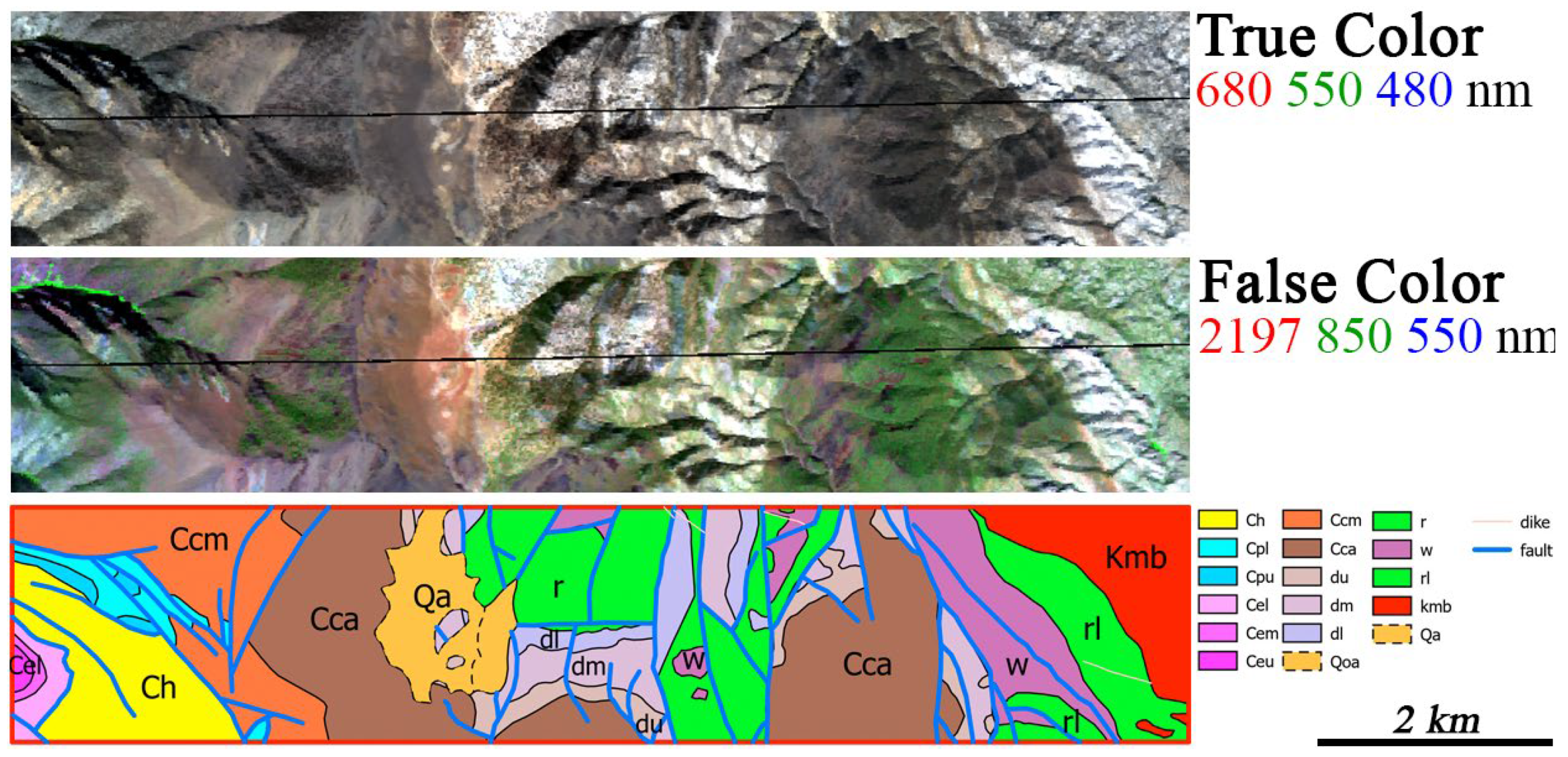
5.2.1. Accurately Mapped Geologic Contacts

This analysis accurately geolocated some bedrock geologic contacts (Figure 8), while others remained elusive. We first discuss the geologic units whose spatial patterns are best described by our analysis, and then we discuss the examples where such patterns are not clearly defined. This contrast informs both the strengths and limitations of the approach.

Map extent of three units in the Schulman Grove study area are well-identified:

• 82 Ma Birch Creek pluton [57]. This intrusive body consists of two rock types, quartz monzonite and granodiorite, and generally consists of a homogeneous bulk chemical composition on the 15-m scale of the AVIRIS data. The pluton does not express any major topographic changes that might result in spatially variable erosion or sediment accumulation that could change the local expression of the rocks exposed at the earth’s surface. Furthermore, this pluton is lithologically unique relative to all other rock types outcropping in the study area—it is an intermediate to felsic plutonic rock.
• Precambrian Reed dolomite [58]. This unit is a gray to buff oolitic carbonate. Its massive coarse-grained texture indicates significant metamorphic recrystallization and significant bulk chemical homogeneity on the spatial scales of a 15-m pixel. This oolite consists predominantly of carbonate minerals, and so its bulk chemistry and mineralogy are almost entirely unique relative to the Birch Creek pluton.
• Cambrian Harkless Formation [58]. This rock unit is a gray-green to brown platy silty shale with thin beds of fine-grained quartzite. This rock type is composed of metamorphosed siliciclastic sediments, and largely lacks carbonate minerals. In terms of bulk chemistry, this unit is highly distinct from the Reed dolomite. In terms of texture, this unit is highly distinct from the Birch Creek pluton.

These three rock units have distinct bulk chemical, mineralogic, and textural manifestations, and so it is not surprising that they are the best constrained rock units in the study area. In contrast, several other rock types in the map area were not so well behaved. We discuss these cases next.

5.2.2. Complex Cases

Several pixel clusters and map units do not uniquely match. This broadly includes three main types, each of which we discuss below:

• Poorly defined general outcrop extent. The best example of this is the magenta pixel cluster, which has its greatest number of pixels concentrated in the lower left corner of Figure 8 (left side, middle panel). At this location, it primarily represents the Cambrian Emigrant Formation, which is composed of mixed limestone, chert, and shale lithologies. Unlike the unique character of the more distinctive units discussed above, this rock unit is highly heterogeneous on the 15-m scale. At several other locations across the map area, this cluster reappears, in particular at the locations of several of the members of the Deep Spring Formation (lower, middle, and upper). These are generally described as mixed carbonate-siliciclastic units composed of carbonates, shale, sandstone, and siltstone. In this case, the Emigrant Formation and Deep Spring Formation have similar chemical, mineralogical, and textural characteristics, which we interpret as the geologic cause for the algorithms grouping them together into a single cluster.
• Imprecise locations of geologic contacts between map units. This type of difference between the geologic bedrock map and the IS results is best exemplified by observing the edges around the Quaternary alluvium (Qal) map unit in the central portion of the study area. These edges are diffuse, consist of multiple different pixel clusters, and generally are not precisely located at the location where they appear on the geologic map [58]. In this case, Qal is a Quaternary alluvium surficial deposit, which represents an accumulation of detritus in a local topographic low area where debris settles after transiting down hillslopes. Due to this, the Qal unit is physically composed of eroded chunks from all of the bedrock units exposed in the surrounding upslope catchment area. This results in some local accumulations of specific rock types from different slopes, grain size sorting based on local topography, and also fine-grained accumulations where standing water may pond and dry up seasonally. This extreme diversity of local geologic processes results in a single map unit (Qal) that is defined based on its very high geologic dimensionality and, therefore, is not well represented as a homogeneous chemical, mineralogical, or textural expression at the earth’s surface. Because of this, it is not surprising that its boundaries are poorly constrained by IS data.
• Internal variation within a unit. The best example of internal variation in map units that confounds accurate algorithmic identification is the Cambrian Campito Formation. This formation outcrops in the map area as two distinct members, the Montenegro Member, gray shale and interbedded quartzite, and the Andrews Mountain Member, massively bedded cross-stratified quartzitic sandstone, siltstone, and shale. In this case, the map unit for each member includes multiple pixel clusters. The lithologically heterogeneous strata that make up these units result in heterogeneity on the pixel scale that confounds the algorithm’s ability to reproduce the boundary designations composed in the geologic map. Additionally, the outcrop extent of these units in the study area is primarily on a steep hillslope that spans approximately 1000 m of the topographic relief. This results in significant erosion at high elevations and accumulations at low elevations that result in map-scale surficial heterogeneity.

The examples discussed here highlight cases where IS analysis succeeds and fails to reproduce bedrock geologic mapping. In many ways, both types of examples meet geologic expectations. The map units with accurate and precise agreement to IS data are clearly distinct in terms of their mineralogy, chemistry, and texture. On the other hand, the lithologies with poor agreement to IS data exist in complex locations where multiple geologic processes interact to complexify the surface observations. Cases such as these require a depth of on-the-ground field observation and interpretation to elucidate the true nature of the bedrock relationships that are standard for a field mapper, but not currently achievable computationally.

For the experienced geologic field worker, this comes as no surprise. The practice of generating geologic maps in the field is intentionally repetitive, redundant, and iterative. Despite the best efforts of geologists, field data often remain nonunique and maps reflect best-guesses and best-practice interpretations based on limited data. In this context, it appears that the level of information extracted by this new IS analysis framework is approaching the field scale of surface observations. This approach is clearly useful for pre-field geologic reconnaissance and base-map utilization. Additionally, as it is further applied and refined, the implications for geologists will surely continue to grow.

6. Conclusions

Using a popular area for geologic field education in the White Mountains, CA, we demonstrate a new approach for the application of imaging spectroscopy for field reconnaissance and boundary delineation of bedrock units. This approach synthesizes two analysis methods: the spectral mixture residual and joint characterization. First, the mixture residual mitigates potentially confounding effects of vegetation cover and terrain in a linear, physically based way. Then, joint characterization identifies spectrally distinct clusters, which may correspond to meaningful geologic differences among and within some rock units. Field validation confirms these spectrally distinct units can partially identify well-established boundaries among geologic map units, as well as refine and contextualize the information conveyed by a geologic map. Once global hyperspectral data are available, this approach could easily be extended to study sites worldwide, offering a step toward efficient and effective use of imaging spectroscopy by field geologists in research, education, and industry.

References

- Bernknopf, R.L.; Brookshire, D.S.; Soller, D.R.; McKee, M.J.; Sutter, J.F.; Matti, J.C.; Campbell, R.H. Societal Value of Geologic Maps; US Geological Survey Circular 111; US Geological Survey Circular: Reston, VA, USA, 1993.
- Winchester, S. The Map That Changed the World: William Smith and the Birth of Modern Geology, 1st ed.; Vannithone, S., Ed.; HarperCollins: New York, NY, USA, 2001; ISBN 0060193611. [Google Scholar]
- Crosthwait, C.H.L. Air Survey and Empire Development. J. R. Soc. Arts 1928, 77, 162–182. [Google Scholar]
- McCurdy, P. Manual of Photogrammetry; Pitman Pub. Corp.: New York, NY, USA; Chicago, IL, USA, 1944. [Google Scholar]
- Fonstad, M.A.; Dietrich, J.T.; Courville, B.C.; Jensen, J.L.; Carbonneau, P.E. Topographic Structure from Motion: A New Development in Photogrammetric Measurement. Earth Surf. Process. Landf. 2013, 38, 421–430. [Google Scholar] [CrossRef] [Green Version]
- Shean, D.E.; Alexandrov, O.; Moratto, Z.M.; Smith, B.E.; Joughin, I.R.; Porter, C.; Morin, P. An Automated, Open-Source Pipeline for Mass Production of Digital Elevation Models (DEMs) from Very-High-Resolution Commercial Stereo Satellite Imagery. ISPRS J. Photogramm. Remote Sens. 2016, 116, 101–117. [Google Scholar] [CrossRef] [Green Version]
- Collis, R. Lidar. Appl. Opt. 1970, 9, 1782–1788. [Google Scholar] [CrossRef] [PubMed]
- Baker, R.N. Landsat Data: A New Perspective for Geology. Photogramm. Eng. Remote Sens. 1975, 41, 1233–1239. [Google Scholar]
- National Academies of Sciences, Engineering, and Medicine. Thriving on Our Changing Planet: A Decadal Strategy for Earth Observation from Space; The National Academies Press: Washington, DC, USA, 2018; ISBN 9780309467575. [Google Scholar]
- Margetta, R. New NASA Earth System Observatory to Help Address Climate Change. Available online: http://www.nasa.gov/press-release/new-nasa-earth-system-observatory-to-help-address-mitigate-climate-change (accessed on 19 August 2021).
- Green, R.O.; Mahowald, N.; Ung, C.; Thompson, D.R.; Bator, L.; Bennet, M.; Bernas, M.; Blackway, N.; Bradley, C.; Cha, J.; et al. The Earth Surface Mineral Dust Source Investigation: An Earth Science Imaging Spectroscopy Mission. In Proceedings of the 2020 IEEE Aerospace Conference, Big Sky, MT, USA, 7–14 March 2020; pp. 1–15. [Google Scholar]
- Candela, L.; Formaro, R.; Guarini, R.; Loizzo, R.; Longo, F. Varacalli the PRISMA Mission. In Proceedings of the 2016 IEEE International Geoscience and Remote Sensing Symposium (IGARSS), Beijing, China, 10–15 July 2016; pp. 253–256. [Google Scholar]
- Nieke, J.; Rast, M. Towards the Copernicus Hyperspectral Imaging Mission for the Environment (CHIME). In Proceedings of the IGARSS 2018—2018 IEEE International Geoscience and Remote Sensing Symposium, Valencia, Spain, 22–27 July 2018; pp. 157–159. [Google Scholar]
- Guanter, L.; Kaufmann, H.; Segl, K.; Foerster, S.; Rogass, C.; Chabrillat, S.; Kuester, T.; Hollstein, A.; Rossner, G.; Chlebek, C. The EnMAP Spaceborne Imaging Spectroscopy Mission for Earth Observation. Remote Sens. 2015, 7, 8830–8857. [Google Scholar] [CrossRef] [Green Version]
- Krutz, D.; Müller, R.; Knodt, U.; Günther, B.; Walter, I.; Sebastian, I.; Säuberlich, T.; Reulke, R.; Carmona, E.; Eckardt, A.; et al. The Instrument Design of the DLR Earth Sensing Imaging Spectrometer (DESIS). Sensors 2019, 19, 1622. [Google Scholar] [CrossRef] [Green Version]
- Iwasaki, A.; Ohgi, N.; Tanii, J.; Kawashima, T.; Inada, H. Hyperspectral Imager Suite (HISUI)-Japanese Hyper-Multi Spectral Radiometer. In Proceedings of the 2011 IEEE International Geoscience and Remote Sensing Symposium, Vancouver, BC, Canada, 24–29 July 2011; pp. 1025–1028. [Google Scholar]
- Clark, R.N.; Swayze, G.A.; Livo, K.E.; Kokaly, R.F.; Sutley, S.J.; Dalton, J.B.; McDougal, R.R.; Gent, C.A. Imaging Spectroscopy: Earth and Planetary Remote Sensing with the USGS Tetracorder and Expert Systems. J. Geophys. Res. E Planets 2003, 108, 1–44. [Google Scholar] [CrossRef]
- Green, R.O.; Eastwood, M.L.; Sarture, C.M.; Chrien, T.G.; Aronsson, M.; Chippendale, B.J.; Faust, J.A.; Pavri, B.E.; Chovit, C.J.; Solis, M. Imaging Spectroscopy and the Airborne Visible/Infrared Imaging Spectrometer (AVIRIS). Remote Sens. Environ. 1998, 65, 227–248. [Google Scholar] [CrossRef]
- Goetz, A.F.H. Three Decades of Hyperspectral Remote Sensing of the Earth: A Personal View. Remote Sens. Environ. 2009, 113, S5–S16. [Google Scholar] [CrossRef]
- Corson, M.R.; Korwan, D.R.; Lucke, R.L.; Snyder, W.A.; Davis, C.O. The Hyperspectral Imager for the Coastal Ocean (HICO) on the International Space Station. In Proceedings of the IGARSS 2008—2008 IEEE International Geoscience and Remote Sensing Symposium 2008, Boston, MA, USA, 7–11 July 2008; Volume 4, pp. IV-101–IV-104. [Google Scholar] [CrossRef]
- Pearlman, J.S.; Barry, P.S.; Segal, C.C.; Shepanski, J.; Beiso, D.; Carman, S.L. Hyperion, a Space-Based Imaging Spectrometer. IEEE Trans. Geosci. Remote Sens. 2003, 41, 1160–1173. [Google Scholar] [CrossRef]
- Asner, G.P.; Knapp, D.E.; Boardman, J.; Green, R.O.; Kennedy-Bowdoin, T.; Eastwood, M.; Martin, R.E.; Anderson, C.; Field, C.B. Carnegie Airborne Observatory-2: Increasing Science Data Dimensionality via High-Fidelity Multi-Sensor Fusion. Remote Sens. Environ. 2012, 124, 454–465. [Google Scholar] [CrossRef]
- Boardman, J.W.; Green, R.O. Exploring the Spectral Variability of the Earth as Measured by AVIRIS in 1999. In Proceedings of the Summaries of the 8th Annual JPL Airborne Geoscience Workshop, Pasadena, CA, USA, 4–8 March 1996; NASA: Pasadena, CA, USA, 2000; Volume 1, pp. 1–12. [Google Scholar]
- Cawse-Nicholson, K.; Hook, S.J.; Miller, C.E.; Thompson, D.R. Thompson Intrinsic Dimensionality in Combined Visible to Thermal Infrared Imagery. IEEE J. Sel. Top. Appl. Earth Obs. Remote Sens. 2019, 12, 4977–4984. [Google Scholar] [CrossRef]
- Thompson, D.R.; Boardman, J.W.; Eastwood, M.L.; Green, R.O. A Large Airborne Survey of Earth’s Visible-Infrared Spectral Dimensionality. Opt. Express 2017, 25, 9186–9195. [Google Scholar] [CrossRef] [PubMed] [Green Version]
- Goetz, A.F.H.; Billingsley, F.C.; Gillespie, A.R.; Abrams, M.J.; Squires, R.L.; Shoemaker, E.M.; Lucchitta, I.; Elston, D.P. Application of ERTS Images and Image Processing to Regional Geologic Problems and Geologic Mapping in Northern Arizona; Technical Report; Jet Propulsion Laboratory: Pasadena, CA, USA, 1975. [Google Scholar]
- Abrams, M.J.; Ashley, R.P.; Rowan, L.C.; Goetz, A.F.H.; Kahle, A.B. Mapping of Hydrothermal Alteration in the Cuprite Mining District, Nevada, Using Aircraft Scanner Images for the Spectral Region 0.46 to 2.36µm. Geology 1977, 5, 713–718. [Google Scholar] [CrossRef]
- Rowan, L.C.; Wetlaufer, P.H.; Stewart, J.H. Discrimination of Rock Types and Detection of Hydrothermally Altered Areas in South-Central Nevada by the Use of Computer-Enhanced ERTS Images; Geological Survey: Washington, DC, USA, 1976.
- Goetz, A.F.H.; Vane, G.; Solomon, J.E.; Rock, B.N. Imaging Spectrometry for Earth Remote Sensing. Science 1985, 228, 1147–1153. [Google Scholar] [CrossRef]
- Clark, R.N.; Roush, T.L. Reflectance Spectroscopy: Quantitative Analysis Techniques for Remote Sensing Applications. J. Geophys. Res. Solid Earth 1984, 89, 6329–6340. [Google Scholar] [CrossRef]
- Clark, R.N. Spectroscopy of Rocks and Minerals, and Principles of Spectroscopy. In Manual of Remote Sensing, Chapter 1; U.S. Geological Survey: Washington, DC, USA, 1999; pp. 1–77. Available online: http://speclab.cr.usgs.gov (accessed on 1 September 2011).
- Hunt, G.R. Spectral Signatures of Particulate Minerals in the Visible and near Infrared. Geophysics 1977, 42, 501–513. [Google Scholar] [CrossRef] [Green Version]
- Kokaly, R.; Clark, R.; Swayze, G.; Livo, K.; Hoefen, T.; Pearson, N.; Wise, R.; Benzel, W.; Lowers, H.; Driscoll, R. Usgs Spectral Library Version 7 Data: Us Geological Survey Data Release; U.S. Geological Survey: Reston, VA, USA, 2017.
- Clark, R.N.; Green, R.O.; Swayze, G.A.; Meeker, G.; Sutley, S.; Hoefen, T.M.; Livo, K.E.; Plumlee, G.; Pavri, B.; Sarture, C.; et al. Environmental Studies of the World Trade Center Area after the September 11, 2001 Attack; Open-File Report; Version 1.1; U.S. Geological Survey: Reston, VA, USA, 2001.
- Clark, R.N.; Swayze, G.A.; Leifer, I.; Livo, K.E.; Lundeen, S.; Eastwood, M.; Green, R.O.; Kokaly, R.F.; Hoefen, T.; Sarture, C.; et al. A Method for Qualitative Mapping of Thick Oil Spills Using Imaging Spectroscopy; Open-File Report; U.S. Geological Survey: Reston, VA, USA, 2010.
- Clark, R.N.; Brown, R.H.; Jaumann, R.; Cruikshank, D.P.; Nelson, R.M.; Buratti, B.J.; McCord, T.B.; Lunine, J.; Baines, K.H.; Bellucci, G.; et al. Compositional Maps of Saturn’s Moon Phoebe from Imaging Spectroscopy. Nature 2005, 435, 66–69. [Google Scholar] [CrossRef]
- Christensen, P.R.; Bandfield, J.L.; Hamilton, V.E.; Howard, D.A.; Lane, M.D.; Piatek, J.L.; Ruff, S.W.; Stefanov, W.L. A Thermal Emission Spectral Library of Rock-Forming Minerals. J. Geophys. Res. Planets 2000, 105, 9735–9739. [Google Scholar] [CrossRef] [Green Version]
- Peyghambari, S.; Zhang, Y. Hyperspectral Remote Sensing in Lithological Mapping, Mineral Exploration, and Environmental Geology: An Updated Review. J. Appl. Remote Sens. 2021, 15, 031501. [Google Scholar] [CrossRef]
- Boardman, J.W.; Kruse, F.A.; Green, R.O. Mapping Target Signatures via Partial Unmixing of AVIRIS Data; Jet Propulsion Laboratory: Pasadena, CA, USA, 1995. [Google Scholar]
- Winter, M.E. N-FINDR: An Algorithm for Fast Autonomous Spectral End-Member Determination in Hyperspectral Data; SPIE: Bellingham, WA, USA, 1999; Volume 3753, pp. 266–275. [Google Scholar]
- Nascimento, J.M.; Dias, J.M. Vertex Component Analysis: A Fast Algorithm to Unmix Hyperspectral Data. IEEE Trans. Geosci. Remote Sens. 2005, 43, 898–910. [Google Scholar] [CrossRef] [Green Version]
- Roger, R. Sparse Inverse Covariance Matrices and Efficient Maximum Likelihood Classification of Hyperspectral Data. Int. J. Remote Sens. 1996, 17, 589–613. [Google Scholar] [CrossRef]
- Gualtieri, J.A.; Cromp, R.F. Support Vector Machines for Hyperspectral Remote Sensing Classification; SPIE: Bellingham, WA, USA, 1999; Volume 3584, pp. 221–232. [Google Scholar]
- Galdames, F.J.; Perez, C.A.; Estévez, P.A.; Adams, M. Rock Lithological Instance Classification by Hyperspectral Images Using Dimensionality Reduction and Deep Learning. Chemom. Intell. Lab. Syst. 2022, 224, 104538. [Google Scholar] [CrossRef]
- Wang, Z.; Tian, S. Lithological Information Extraction and Classification in Hyperspectral Remote Sensing Data Using Backpropagation Neural Network. PLoS ONE 2021, 16, e0254542. [Google Scholar] [CrossRef]
- Doshi-Velez, F.; Kim, B. Towards a Rigorous Science of Interpretable Machine Learning. arXiv 2017, arXiv:1702.08608. [Google Scholar]
- Fanelli, D. Is Science Really Facing a Reproducibility Crisis, and Do We Need It To? Proc. Natl. Acad. Sci. USA 2018, 115, 2628–2631. [Google Scholar] [CrossRef] [Green Version]
- Knight, W. The Dark Secret at the Heart of AI. Available online: https://www.technologyreview.com/2017/04/11/5113/the-dark-secret-at-the-heart-of-ai/ (accessed on 3 March 2022).
- Molnar, C. Interpretable Machine Learning. A Guide for Making Black Box Models Explainable; LuLu: Morisville, NC, USA, 2019. [Google Scholar]
- Small, C. Grand Challenges in Remote Sensing Image Analysis and Classification. Front. Remote Sens. 2021, 1, 605220. [Google Scholar] [CrossRef]
- Sousa, D.; Brodrick, P.G.; Cawse-Nicholson, K.; Fisher, J.B.; Pavlick, R.; Small, C.; Thompson, D.R. The Spectral Mixture Residual: A Source of Low-Variance Information to Enhance the Explainability and Accuracy of Surface Biology and Geology Retrievals. J. Geophys. Res. Biogeosci. 2022, 127, e2021JG006672. [Google Scholar] [CrossRef]
- Sousa, D.; Small, C. Joint Characterization of Multiscale Information in High Dimensional Data. Adv. Artif. Intell. Mach. Learn. 2021, 1, 196–212. [Google Scholar] [CrossRef]
- Small, C.; Sousa, D. Joint Characterization of the Cryospheric Spectral Feature Space. Front. Remote Sens. 2021, 2, 793228. [Google Scholar] [CrossRef]
- Sousa, D.; Small, C. Joint Characterization of Spatiotemporal Data Manifolds. Front. Remote Sens. 2022, 3, 760650. [Google Scholar] [CrossRef]
- Corsetti, F.A.; Hagadorn, J.W. Precambrian-Cambrian Transition: Death Valley, United States. Geology 2000, 28, 299–302. [Google Scholar] [CrossRef]
- Nelson, C.A.; Sylvester, A.G. Wall Rock Decarbonation and Forcible Emplacement of Birch Creek Pluton, Southern White Mountains, California. GSA Bull. 1971, 82, 2891–2904. [Google Scholar] [CrossRef]
- Dilles, J.H.; Barton, M.D.; Johnson, D.A.; Proffett, J.M.; Einaudi, M.T.; Crafford, E.J. Part I. Contrasting Styles of Intrusion-Associated Hydrothermal Systems: Part II. Geology & Gold Deposits of the Getchell Region; Society of Economic Geologists: Littleton, CO, USA, 2000; ISBN 9781934969854. [Google Scholar]
- Nelson, C.A. Geologic Map of the Blanco Mountain Quadrangle, Inyo and Mono Counties, California; Geologic Quadrangle: Sierra County, NM, USA, 1966. [Google Scholar]
- Ferguson, C.W. A 7104-Year Annual Tree-Ring Chronology for Bristlecone Pine, Pinus Aristata, from the White Mountains, California; Tree-Ring Society: Ndola, Zambia, 1969. [Google Scholar]
- Stockli, D.F.; Dumitru, T.A.; McWilliams, M.O.; Farley, K.A. Cenozoic Tectonic Evolution of the White Mountains, California and Nevada. GSA Bull. 2003, 115, 788–816. [Google Scholar] [CrossRef]
- LaMarche, V.C. Holocene Climatic Variations Inferred from Treeline Fluctuations in the White Mountains, California. Quat. Res. 1973, 3, 632–660. [Google Scholar] [CrossRef]
- Stockli, D.F.; Farley, K.A.; Dumitru, T.A. Calibration of the Apatite (U-Th)/He Thermochronometer on an Exhumed Fault Block, White Mountains, California. Geology 2000, 28, 983–986. [Google Scholar] [CrossRef]
- Tang, K.; Feng, X.; Funkhouser, G. The Δ13C of Tree Rings in Full-Bark and Strip-Bark Bristlecone Pine Trees in the White Mountains of California. Glob. Chang. Biol. 1999, 5, 33–40. [Google Scholar] [CrossRef]
- Pace, N. White Mountain Research Station: 25 Years of High-Altitude Research; University of California: Berkley, CA, USA, 1973. [Google Scholar]
- Nelson, C.A.; Durham, J.W. Guidebook for Field Trip to Precambrian-camrian Succession White-Inyo Mountains, California; University of California: Los Angeles, CA, USA, 1966. [Google Scholar]
- Bentley, C. Friday Folds: The Poleta Folds. In Mountain Beltway; American Geophysical Union: Washington, DC, USA, 2012. [Google Scholar]
- Swayze, G.; Clark, R.N.; Kruse, F.; Sutley, S.; Gallagher, A. Ground-Truthing AVIRIS Mineral Mapping at Cuprite; University of Colorado at Boulder: Denver, CO, USA, 1992. [Google Scholar]
- Goetz, A.F.; Vane, G. Mineralogical Mapping in the Cuprite Mining District, Nevada. In Proceedings of the Airborne Imaging Spectrometer Data Analysis Workshop, Pasadena, CA, USA, 8–10 April 1985. [Google Scholar]
- Kruse, F.; Kierein-Young, K.; Boardman, J. Mineral Mapping at Cuprite, Nevada with a 63-Channel Imaging Spectrometer. Photogramm. Eng. Remote Sens. 1990, 56, 83–92. [Google Scholar]
- Swayze, G.A. The Hydrothermal and Structural History of the Cuprite Mining District, Southwestern Nevada: An Integrated Geological and Geophysical Approach. Ph.D. Thesis, University of Colorado at Boulder, Denver, CO, USA, 1997. [Google Scholar]
- Gao, B.-C.; Heidebrecht, K.B.; Goetz, A.F.H. Derivation of Scaled Surface Reflectances from AVIRIS Data. Remote Sens. Environ. 1993, 44, 165–178. [Google Scholar] [CrossRef]
- Thompson, D.R.; Natraj, V.; Green, R.O.; Helmlinger, M.C.; Gao, B.-C.; Eastwood, M.L. Optimal Estimation for Imaging Spectrometer Atmospheric Correction. Remote Sens. Environ. 2018, 216, 355–373. [Google Scholar] [CrossRef]
- Boardman, J.W. Automating Spectral Unmixing of AVIRIS Data Using Convex Geometry Concepts; University of Colorado at Boulder: Denver, CO, USA, 1993; Volume 1, pp. 11–14. [Google Scholar]
- Small, C. The Landsat ETM+ Spectral Mixing Space. Remote Sens. Environ. 2004, 93, 1–17. [Google Scholar] [CrossRef]
- Small, C.; Milesi, C. Multi-Scale Standardized Spectral Mixture Models. Remote Sens. Environ. 2013, 136, 442–454. [Google Scholar] [CrossRef] [Green Version]
- Sousa, D.; Small, C. Global Cross-Calibration of Landsat Spectral Mixture Models. Remote Sens. Environ. 2017, 192, 139–149. [Google Scholar] [CrossRef] [Green Version]
- Sousa, D.; Small, C. Globally Standardized MODIS Spectral Mixture Models. Remote Sens. Lett. 2019, 10, 1018–1027. [Google Scholar] [CrossRef]
- Small, C. Multisource Imaging of Urban Growth and Infrastructure Using Landsat, Sentinel and SRTM. In NASA Landsat-Sentinel Science Team Meeting; NASA: Rockville, MD, USA, 2018. [Google Scholar]
- Sousa, D.; Small, C. Multisensor Analysis of Spectral Dimensionality and Soil Diversity in the Great Central Valley of California. Sensors 2018, 18, 583. [Google Scholar] [CrossRef] [Green Version]
- Sousa, D.; Small, C. Linking Common Multispectral Vegetation Indices to Hyperspectral Mixture Models: Results from 5 Nm, 3 m Airborne Imaging Spectroscopy in a Diverse Agricultural Landscape. arXiv 2022, arXiv:2208.06480. [Google Scholar]
- Roberts, D.A.; Gardner, M.; Church, R.; Ustin, S.; Scheer, G.; Green, R.O. Mapping Chaparral in the Santa Monica Mountains Using Multiple Endmember Spectral Mixture Models. Remote Sens. Environ. 1998, 65, 267–279. [Google Scholar] [CrossRef]
- Gillespie, A. Interpretation of Residual Images: Spectral Mixture Analysis of AVIRIS Images, Owens Valley, California. In Proceedings of the Second Airborne Visible/Infrared Imaging Spectrometer (AVIRIS) Workshop, Pasadena, CA, USA, 4–5 June 1990; NASA: Pasadena, CA, USA, 1990; pp. 243–270. [Google Scholar]
- Garcia, M.; Ustin, S.L. Detection of Interannual Vegetation Responses to Climatic Variability Using AVIRIS Data in a Coastal Savanna in California. IEEE Trans. Geosci. Remote Sens. 2001, 39, 1480–1490. [Google Scholar] [CrossRef]
- Small, C.; Sousa, D. The Climatic Temporal Feature Space: Continuous and Discrete. Adv. Artif. Intell. Mach. Learn. 2021, 1, 165–183. [Google Scholar] [CrossRef]
- Hunt, G.R.; Ashley, R.P. Spectra of Altered Rocks in the Visible and near Infrared. Econ. Geol. 1979, 74, 1613–1629. [Google Scholar] [CrossRef]
- Van der Maaten, L.; Hinton, G. Visualizing Data Using T-SNE. J. Mach. Learn. Res. 2008, 9, 2579–2605. [Google Scholar]
- McInnes, L.; Healy, J.; Melville, J. UMAP: Uniform Manifold Approximation and Projection for Dimension Reduction. arXiv 2020, arXiv:1802.03426. [Google Scholar]
- Sousa, F.J.; Sousa, D.J. Spatial Patterns of Chemical Weathering at the Basal Tertiary Nonconformity in California from Multispectral and Hyperspectral Optical Remote Sensing. Remote Sens. 2019, 11, 2528. [Google Scholar] [CrossRef] [Green Version]
- Candès, E.J.; Li, X.; Ma, Y.; Wright, J. Robust Principal Component Analysis? JACM 2011, 58, 1–37. [Google Scholar] [CrossRef]
Publisher’s Note: MDPI stays neutral with regard to jurisdictional claims in published maps and institutional affiliations. |
© 2022 by the authors. Licensee MDPI, Basel, Switzerland. This article is an open access article distributed under the terms and conditions of the Creative Commons Attribution (CC BY) license (https://creativecommons.org/licenses/by/4.0/).
Share and Cite
Sousa, F.J.; Sousa, D.J. Hyperspectral Reconnaissance: Joint Characterization of the Spectral Mixture Residual Delineates Geologic Unit Boundaries in the White Mountains, CA. Remote Sens. 2022, 14, 4914. https://doi.org/10.3390/rs14194914
Sousa FJ, Sousa DJ. Hyperspectral Reconnaissance: Joint Characterization of the Spectral Mixture Residual Delineates Geologic Unit Boundaries in the White Mountains, CA. Remote Sensing. 2022; 14(19):4914. https://doi.org/10.3390/rs14194914
Chicago/Turabian StyleSousa, Francis J., and Daniel J. Sousa. 2022. "Hyperspectral Reconnaissance: Joint Characterization of the Spectral Mixture Residual Delineates Geologic Unit Boundaries in the White Mountains, CA" Remote Sensing 14, no. 19: 4914. https://doi.org/10.3390/rs14194914