1. Introduction
Hyperspectral remote sensing is a technology for continuous remote sensing imaging of ground objects with narrow and continuous spectral channels, which essentially changes the traditional remote sensing monitoring targets and enables the direct detection of undetectable substances in wide-band remote sensing. Mineral mapping is a key application direction in hyperspectral remote sensing in geological and mineral exploration, especially for hydrothermal alteration minerals that indicate prospecting, such as white mica group minerals (which have different aluminum contents), chlorite group minerals (which have different aluminum, magnesium and iron contents), and carbonate minerals [
1,
2,
3,
4]. The identification of altered minerals is critical in regional mineral surveys.
In essence, each pixel spectrum in a hyperspectral remote sensing image is a mixed spectrum, and a set of mineral abundance maps is the final product of the hyperspectral remote sensing processing chain. However, many geological surveyors do not understand the abundance map, and they believe that a distribution map of minerals (especially altered minerals) makes them more convenient to use in the field. Technically, remote sensing mineral mapping is to identify the dominant minerals in each pixel of the image and display their spatial distribution, which belongs to the category of object detection.
In geological remote sensing, there are two broad categories of analytical techniques that are used widely for mineral mapping of hyperspectral remote sensing images: spectrum matching techniques and subpixel methods [
5]. The spectrum matching techniques strive to find a measure of mathematical or physical similarity between a known reference spectrum and an unknown test (target) spectrum. Representative methods include spectral angle mapper (SAM), cross-correlogram spectral matching (CCSM), spectral information divergence (SID), etc. [
6]. However, the major problem associated with similarity measures is their inability to deal with mixed spectra as well as subjective thresholding [
7]. Subpixel methods comprise techniques to unmix hyperspectral images with the aim of quantifying the relative abundance of various materials within a pixel. The mixture-tuned matched filtering (MTMF) is a typical subpixel method that is often used to generate mineral abundance maps [
8]. Their output is a single score or percent per pixel, which bear some resemblance to similarity measures, leading to the threshold problem that still exists for mineral mapping using the subpixel method.
In real geological environments, there is a complex mixture of minerals with similar spectra. In such cases, distinctive absorption features happen very close to or overlap with each other and relevant spectra are highly correlated. This correlation hinders any attempts to identify or discriminate the minerals in routine ways. The discrimination of spectrally similar and intimately mixed minerals and prediction of their abundances in the mixture are long-standing issues in mineral mapping. The polynomial fitting method can effectively track the changes in wavelength positions related to component changes, such as Al-OH and Mg-OH [
9,
10]. However, this method is mainly applied to composition mapping of specific mineral types. It is obviously more appealing to map various types of minerals simultaneously, including mineral subtypes with similar spectra and different components, in a single remote sensing image.
In recent years, machine learning methods, as a subdomain of artificial intelligence, have been increasingly introduced into remote sensing geology or mineral exploration, including support vector machine (SVM), random forest (RF), and artificial neural network (ANN) [
11,
12,
13,
14]. Machine learning methods are data-driven and can automatically learn the relationship between spectral data and desired features. Moreover, these methods are robust in processing spectral data against noise and uncertainties, and can reliably analyze and efficiently classify hyperspectral remote sensing image data [
15,
16].
In the field of machine learning, deep learning is currently the most focused technology due to its achievements in speech recognition, visual object recognition, object detection and various other domains [
17,
18,
19]. Deep learning is a method of feature learning through deep neural networks (DNNs). Some scholars have introduced deep learning into hyperspectral image classification, achieving high classification accuracies of more than 90% or even 95% [
20,
21,
22,
23,
24,
25,
26]. Although the above studies have demonstrated that deep learning can improve the classification accuracy of ground objects in hyperspectral images, most of the studied objects were stable and uniform artificial ground objects in farmland, woodland or water, which are considerably different from minerals in geological environments.
To date, there are a few studies concerned with the application of deep learning in processing remote sensing data for mineral exploration [
16]. In the past two years, some scholars have used deep learning technology to identify minerals from hyperspectral images or spectral data of rock samples obtained under laboratory conditions. For example, Okada et al. proposed an automatic mineral identification system based on a deep learning method, and established a convolutional neural network (CNN) model for deep learning of 400–1000 nm hyperspectral data obtained by a Specim hyperspectral camera, which greatly improved the classification accuracy of five types of minerals: galena, chalcopyrite, hematite with large particles, hematite with small particles, and hematite with very small particles [
27]. Jahoda et al. used machine learning methods including CNNs, to evaluate the mineral classification accuracy of different spectral data measured in the laboratory (Raman spectra, visible-near infrared spectra and laser spectra), and the results demonstrated that machine learning techniques can successfully combine the spectra of two analytical instruments to improve mineral classification accuracy [
28]. Zeng et al. designed a spatial-spectral residual CNN that can successfully detect minerals from hyperspectral images. Unfortunately, the accuracy assessments of specific minerals are not shown [
29]. In summary, for mineral mapping of hyperspectral remote sensing images, the application of deep learning has not yet been fully explored, and this research aims to contribute to its advancement in geological remote sensing. Whether deep learning methods can improve hyperspectral image mineral identification, especially for the discrimination of spectrally similar and intimately mixed minerals, requires further evaluation.
The Baiyanghe uranium deposit is a typical hydrothermal uranium deposit in Northwestern Xinjiang, China, which is comprised of a rich variety of altered minerals with little vegetation cover, thus providing a suitable target for hyperspectral remote sensing mineral mapping. In this research, the Baiyanghe uranium deposit is also a suitable test area for evaluating hyperspectral remote sensing mineral mapping based on DNN methods. The reasons are as follows: First, this area is rich in white mica group minerals. The spectral characteristics of its subtypes are very similar and often mixed with each other, which allows us to test the ability of deep learning methods to distinguish these mineral subtypes. Second, we carried out airborne hyperspectral remote sensing measurements in this area, and obtained mineral mapping results based on the MTMF method, which can be used to compare the new results [
30]. Most importantly, we conducted extensive field investigations and spectral measurements in this area, and the ground spectra collected can be used to validate airborne hyperspectral identification results [
2,
31].
In addition to the deep learning method, we also use some other methods in the field of machine learning for comparison in the experiment, such as the SVM method in supervised classification, which has achieved good results in remote sensing lithology classification [
32,
33]. In the design of the DNN model, we also use more than one model structure to test, evaluate, and compare their accuracy and mapping effect, providing a reference for the future application of deep learning technology in hyperspectral remote sensing mineral mapping.
3. Methodology
3.1. Working Method
The working process of this research includes airborne hyperspectral data processing, sample dataset construction, deep learning and its applications, as shown in
Figure 3. Airborne hyperspectral data processing includes a series of preprocessing processes, where radiometric calibration and ortho-corrections are performed by ITRES software, and atmospheric corrections and elimination of bad bands are performed by ENVI software (version 5.3) developed by Exelis Visual Information Solutions (EVIS), Boulder, CO, USA.
Considering the different scales of ground data and airborne hyperspectral data, we use airborne scale data as samples. The sample dataset is constructed based on MTMF mapping results validated with ground truth data from previous studies, and each type of mineral was examined by spectral inspection to ensure its reliability. When all the samples were labeled, the sample dataset was divided into training, validation and test sets at a ratio of 6:2:2. Sixty percent of the samples were used to train the DNN model. Twenty percent of the samples were used as the validation set for feedback of the output result of training. Twenty percent of the samples were used as the test set and did not participate in training; these samples were applied to evaluate the generalization capability of the DNN model.
Then, three DNNs were designed according to the characteristics of the airborne hyperspectral data in the PyTorch deep learning framework. In this study, the fully connected neural network (FCNN) and CNN were used as the basic architecture. FCNNs and CNNs are the two most widely used network structures in deep learning. In general, CNNs are more suitable for processing images than FCNNs [
23,
38]. However, hyperspectral images are considerably different from general RGB images, as hyperspectral images combine images with spectra. Since the spectral resolution of hyperspectral images is very high, these images can be used not only to identify ground objects with large spectral features in a group of ground objects, but also to theoretically distinguish ground objects with slight spectral differences in groups of ground objects through feature mining. Therefore, an FCNN was still considered in our experiments, and the results were compared with those of a CNN. Because airborne hyperspectral data have both high spectral resolution and high spatial resolution, two structures of CNNs were designed for this study. One is the 1D CNN based on the spectral information, and the other is the 1D and 2D CNN considering the spectral and spatial information.
The model was trained on the training set and validated on the test set of the sample dataset, and then the model was established according to the accuracy results. Finally, the model was applied to identify minerals in airborne hyperspectral images of the test area, and the mapping results were verified and evaluated based on the ground truth data. In addition, to increase the contrast, SVM as a competitor, using the same training set for supervised learning, was applied to the airborne hyperspectral mineral mapping in the test area.
The DNN models applied in this study are based on the Python language and PyTorch deep learning framework. The program design, code writing, debugging and running processes were carried out in the PyCharm integrated development environment.
3.2. Hyperspectral Remote Sensing Data Preprocessing
The radiometric and geometric corrections of the SASI data were performed using preprocessing software provided by ITRES. Because the Baiyanghe mining area has certain topographic fluctuations, the SASI data were orthorectified in combination with digital elevation model data. The empirical line method was used for atmospheric corrections, and a regression equation was established based on the synchronous hyperspectral data of standard calibrated light and dark materials. After radiometric and atmospheric corrections, the DN values of the SASI hyperspectral images were converted to reflectance values. Finally, the abnormal values affected by water vapor absorption near 1400 nm and 1900 nm and beyond 2420 nm were removed. The removed bands included 9 bands at 1340–1460 nm, 12 bands at 1790–1970 nm and 3 bands beyond 2420 nm, yielding a total of 76 bands.
3.3. Construction of the Mineral Sample Dataset
The deep learning task requires a suitable sample dataset to mine feature information in the data and abstract advanced information to map to the output. When DNNs are applied to identify minerals in airborne hyperspectral images, sample datasets of various minerals for feature mining must be established. Deep learning technology operates as a black box that provides stable processing through a large number of inputs and given results. Therefore, the greater the number of training samples, the more stable and better the working performance of the black box [
39]. In addition to a large number of samples, deep learning methods need to ensure the reliability of the samples.
In theory, ground truth data are the most reliable. However, deep learning has a great demand for the number of samples, and there is a direct scale difference between ground data and airborne hyperspectral data. Therefore, we use the image spectrum to construct a sample dataset. In previous studies, SASI hyperspectral mineral mapping in the Baiyanghe mining area was completed by using the MTMF method, and the mapping results were verified in a certain amount in the field [
30,
31]. To improve the efficiency of sample selection various mineral samples were selected based on the MTMF mapping results (
Figure 4a,c). All selected samples are from one of two images in the test area, as shown in
Figure 4b,d. In the process, the locations of ground truth data obtained by the FieldSpec4 ASD spectrometer were used to guide sample selection, and errors were eliminated pixel by pixel through visual spectral inspection according to the spectral curve shape and wavelength of the absorption peak. A total of 13,186 pixel samples were inspected, of which 11,074 pixels were accurately identified by the MTMF method; therefore, the mineral mapping accuracy of this method was estimated to be 84%.
Five types of altered minerals were sampled in the Baiyanghe area,
Figure 4e shows the spectral curves of minerals measured by an ASD spectrometer. The spectra at point 1 were interpreted as calcite in carbonate minerals, which exhibits one absorption feature near 2338 nm. The spectra at point 2 were interpreted as montmorillonite, which exhibits one absorption feature near 2208 nm. The spectra at point 3 were interpreted as chlorite and epidote, which are often mixed with each other. Chlorite and epidote exhibit two absorption features near 2255 nm and 2340 nm. Through visual spectral inspection, we found that the corresponding pixel spectrum is closer to the spectrum of chlorite (possibly mixed with a small amount of epidote), so the sample is named chlorite. The spectra at points 4 and 5 were interpreted as medium-wavelength white mica, which exhibits two absorption features near 2205 nm and 2350 nm. The spectra at point 6 were interpreted as short-wavelength white mica, which exhibits two absorption features near 2198 nm and 2344 nm. The feature difference between the two types of white mica is mainly reflected in the different wavelength positions of Al-OH near 2200 nm. Each class of minerals in the sample dataset was assigned a code or label that was expressed in the numbers 1–5.
The sample dataset also includes the image backgrounds in addition to the five types of mineral samples. Obviously, the number of background pixels substantially exceeds the sum of the five kinds of mineral pixels. If all nonmineral pixels are input into the DNN model as background samples, due to the large gap between the number of mineral samples and the number of background samples, it may lead to difficulties in training the neural network or poor effects while testing the model. According to the number of pixels of the five types of mineral samples and the total number of pixels, the background spectrum was sampled by extracting the pixel spectra from the image at certain intervals to construct a preliminary background spectrum library. Then, the position of the preliminarily collected background samples was inspected in the image, the background samples that overlapped with the mineral samples were eliminated, and the remaining samples were taken as the final background samples.
The number of samples selected for this experiment is shown in
Table 2. The average spectral curves of six kinds of objects in the sample dataset were calculated. As shown in
Figure 5, the main characteristic absorption peaks of the average spectral curves of various minerals after 2000 nm are roughly consistent with the ground truth spectra, indicating that the selected samples are representative and reliable. Because the spectral resolution of SASI airborne hyperspectral data is 15 nm, the absorption peak wavelength position of some minerals deviates from that of the ground truth spectrum; however, the deviation range is within 5 nm. In addition, the average background spectra are considerably different from the spectra of all minerals.
3.4. Deep Neural Network Model Design
3.4.1. FCNN
A DNN is a generalized concept that includes FCNNs, CNNs, and recurrent neural networks (RNNs). A narrow DNN has a fully connected neuron structure; that is, a narrow DNN is an FCNN. An FCNN is a simplified abstraction of the human brain structure and operation mechanism. Each node in an FCNN has an operational relationship with all nodes in the next layer. An FCNN includes a multilayer perceptron that identifies the most reasonable and robust hyperplane between classes [
40]. FCNNs include an input layer, hidden layer and output layer, and the hidden layer can contain multiple layers.
As an important deep learning algorithm, the FCNN was used as one of the basic structures for mineral identification in airborne hyperspectral data in this study. The structure of the FCNN is shown in
Figure 6. By considering factors such as the number of samples, the model complexity, the calculation time and ensuring that the parameters were not overfit, the hidden layer included four layers, and the number of neurons in each layer was set to 128, 256, 256 and 64. The number of neurons in the input layer was set to the number of bands of the spectral data, and the number of neurons in the output layer was set to the number of categories in the sample dataset. The softmax function was used in the last layer of the entire network. The ReLU function was used as the activation function for the hidden layers.
The activation function is an important tool for realizing nonlinear neural networks. In the absence of an activation function, the input to each layer of nodes is a linear combination of the outputs of the previous layer, which is similar to the most primitive perceptron, severely limiting the approximation and fitting abilities of the network. Thus, nonlinear functions were introduced as activation functions to ensure that neural networks can approximate almost any function and can better address nonlinear problems. Typical activation functions include the sigmoid, tanh, and ReLU activation functions. Sigmoid and tanh are saturated activation functions that often lead to the vanishing gradient problem, making it difficult to train neural network models [
41]. To solve this problem, Krizhevsky et al. proposed ReLU, a nonsaturated activation function, and achieved excellent results in the ImageNet ILSVRC competition [
42]. Compared with the sigmoid and tanh functions, the ReLU function has good sparsity and small amount of calculation. It not only avoids gradient disappearance, but also speeds up network training [
43,
44]. Therefore, the ReLU function quickly becomes the mainstream activation function commonly used in deep learning.
3.4.2. CNN
A CNN is a traditional model and representative algorithm in the field of deep learning that is mainly used in image pattern recognition tasks. At present, CNNs play a critical role in the field of computer vision [
45]. A CNN is a kind of feedforward neural network that includes convolution calculations and a deep structure. A CNN consists of a stack of alternating convolution layers and pooling layers. At the end of the network, several fully connected layers are usually used as classifiers. In the convolutional layers, image patches with spatial context information are convoluted with a set of kernels. Then, the pooling layers reduce the size of the feature maps generated by the convolutional layers to obtain more general and abstract features. Finally, the feature maps are transformed into feature vectors by several fully connected layers [
23,
46].
Two CNN structures were designed: the 1D CNN based on the spectral information and the 1D and 2D CNN considering the spectral and spatial information. The structure of the 1D CNN is shown in
Figure 7. The spectral features are extracted through several alternating 1D convolutional layers and pooling layers, and a fully connected layer is used for classification. The structure of the 1D and 2D CNN is shown in
Figure 8. The spatial features are extracted by adding a series of alternating 2D convolution layers and pooling layers and fused with the spectral features extracted by the 1D convolution layers. Finally, a fully connected layer is used for classification.
The CNN model also uses ReLU as its activation function. The convolution kernel sizes of the convolution layers are set to 3 × 3 and 2 × 2 in turn. The pooling layer uses the commonly used maximum pooling method. The concat method in PyTorch is used to fuse the spatial and spectral features in the neural network with 1D and 2D convolutions. The softmax function is used in the last layer of the entire network.
Due to the high spatial resolution of airborne hyperspectral images, they contain rich spatial texture information. However, the data correlations between adjacent hyperspectral bands are high. Thus, in the convolution operation, if all pixels in the hyperspectral band data are taken as inputs to the model, the calculation costs are considerable. Therefore, before spatial information is extracted from the hyperspectral images, the dimensionality of the original hyperspectral images must be reduced. Principal component analysis (PCA) is used to reduce the dimensions of the SASI images. This method uses the variance as an information measure to extract features from the original data [
47]. Principal component analyses and eigenvalue calculations were performed on the preprocessed SASI images. The results show that the first principal component contained 98% of the information in the whole image, the second principal component contained 1% of the information, and the third principal component contained only a few thousandths of the information in the image.
Figure 9 shows the first twenty principal component images after principal component analysis of the SASI image. From these images, the texture of the first principal component image is the most complex and rich; by the 13th principal component image, it is difficult to see the original spatial contour information; by the 17th principal component image, the spatial information is almost blurred. Therefore, to retain as much spatial information as possible, the first sixteen principal components after PCA of the SASI image were input into the 2D CNN for spatial feature extraction. The input principal components contain 99.99% of the information.
3.5. Model Training and Validation
Every machine learning algorithm has an objective function, and the solution process of the algorithm involves optimizing this objective function. In classification or regression problems, the loss function is usually used as the objective function of the model. The loss function evaluates the difference between the predicted and true values of the model. Different deep learning tasks use various objective functions. For example, in regression tasks, the mean squared error loss function is commonly used, while classification tasks typically apply the cross-entropy loss function. At present, the cross-entropy loss function is the most commonly used classification loss function in convolutional neural networks [
48]. Therefore, in this study, the cross-entropy loss function was applied in the neural network models.
The neural network model continuously optimized its parameters through training. The network parameters usually refer to the connection weights between neurons. Deep neural networks gradually adjust the connection weights of each neuron by repeatedly training the known information in the input sample dataset to “learn” the relationship between the input and output data. During the training process, the neural network measures the distance between the output and the expected value through the loss function after initializing the output and uses this distance value as a feedback signal to adjust the weight value and reduce the loss value of the current example. The training process implements the backpropagation algorithm. The algorithm for updating parameters is usually called an optimizer, and the most commonly used optimizer is the gradient descent algorithm. Thus, the neural network was trained by combining the backpropagation algorithm and the gradient descent method.
Before model training, the sample dataset was divided into a training set, a validation set and a test set at a ratio of 6:2:2. Considering that the activation function used in DNN models is ReLU, Kaiming initialization was used to initialize the parameters of the DNNs [
49]. In terms of the parameter settings of the model training process, the batch size was set to 64, the learning rate was set to 0.001, the number of training epochs was set to 2000, and the optimizer was Adam, which adaptively adjusts the learning rate and has high computational efficiency [
50]. After each training epoch, the model performance was evaluated by using the validation set.
Considering the differences in the experimental results of the three DNN models in the Baiyanghe uranium mining area, to evaluate the performance of these models, several evaluation indices were used to assess the accuracy of the models. The indices used in this paper include the overall accuracy, producer’s accuracy, average accuracy and Kappa coefficient, which are important evaluation indices for remote sensing classification models [
51,
52].
The overall accuracy is defined as the ratio of the number of correctly classified samples to the total number of samples. The producer’s accuracy is defined as the probability that the true reference data of each category are correctly classified, which can be calculated as the number of correctly classified samples divided by the total number of samples in each category. The average accuracy is defined as the average of the producer’s accuracies of all categories, which reduces accuracy deviations caused by unbalanced numbers of samples. The Kappa coefficient is a statistics indicator that measures the consistency between two variables. When the two variables are replaced by the classification results and true values, the Kappa coefficient can be used to evaluate model accuracy. In general, the Kappa coefficient varies between 0 and 1, and the larger the Kappa value is, the higher the classification accuracy. In the training process, with the increase in training epochs, the accuracies of the models on the training set and the validation set were observed to judge whether the model was overfitting. According to the accuracies of the models on the validation set, the hyperparameters can be adjusted to obtain better model performance. In this study, we only adjusted the learning rates of the three DNN models, respectively, and obtained good model performance. As shown in
Figure 10, the training and validation accuracies of the three models were all more than 90%. Each network model converged, and the final training and validation accuracies are shown in
Table 3. Among the three models, the 1D and 2D CNN had the highest training accuracy and validation accuracy of 97.039% and 93.003%, respectively.
After the model training was completed, the test set was used to evaluate the final performance of the models. For a more comprehensive evaluation, confusion matrix was used to standardize the classification results and calculate the accuracy index. Each column in the confusion matrix represents a prediction category, and the sum of each column represents the total number of data points predicted for that category. Each row represents the true data category, and the sum of each row represents the number of data instances in that category. Based on the confusion matrix, the correct and incorrect classification ratios of each category can be calculated.
As the final purpose of the application of the DNN model, to better verify its practical effect in hyperspectral remote sensing mineral mapping, the trained DNN models were used to perform mineral identification in the SASI airborne hyperspectral images of the Baiyanghe uranium mining area, and the mineral identification results were output by the models. The results were visualized through the ArcGIS software platform to realize mineral mapping.
4. Results
4.1. Model Evaluation
Table 4 and
Table 5 show various evaluation indices for the three DNN models on the test dataset and show the corresponding indices of the SVM on the test dataset after supervised learning on the training set. The overall accuracy of the three DNN models was more than 90% and is consistent with their accuracy ranking on the training set and the validation set, showing the good stability and generalization capability of these models. In terms of the various indices, the 1D and 2D CNN has the best performance. The overall accuracy of this model is 94.77%, the average accuracy is 94.23%, and the Kappa coefficient is 0.9477, which is higher than the values of the other models. In contrast, the overall accuracy, average accuracy and Kappa coefficient of the SVM are lower than those of the three DNN models, indicating that the deep learning method has better overall performance in this experiment.
For specific categories, the producer’s accuracies of calcite and background in the four methods are high, all greater than 95%, so the errors mainly come from the other four categories. For each method tested, the producer’s accuracy of short-wavelength white mica is the lowest among all categories, indicating that it is the main source of error for each method. The producer’s accuracies of chlorite and short-wavelength white mica of SVM are lower than 70%, which affects its overall accuracy. The case of the FCNN model is similar to that of the SVM. With the exception of short-wavelength white mica, the producer’s accuracies of the other categories of the 1D and 2D CNN model are more than 90%, and the producer’s accuracy of short-wavelength white mica is close to 90%, indicating that the model has a relatively balanced identification ability in this region. The 1D CNN model is somewhat partial. Although the producer’s accuracies of other categories of the model are more than 90% or close to 90%, the producer’s accuracy of short-wavelength white mica is only 80%.
The confusion matrices of the three DNN models and SVM on the test dataset are shown in
Figure 11. The confusion matrices of the models on the test dataset show that the model errors are mainly due to the misclassification of certain categories. The errors in the FCNN model are due to the misclassification of chlorite as the background, the mutual misclassification of short-wavelength white mica and medium-wavelength white mica, and the misclassification of short-wavelength white mica as montmorillonite. The main misclassification errors in the 1D CNN model are due to the misclassification of chlorite as the background and mutual misclassification between short-wavelength white mica and medium-wavelength white mica. The main misclassification errors in the 1D and 2D CNN model are due to the mutual misclassification between short-wavelength white mica and medium-wavelength white mica. The main misclassification errors in the SVM method are due to the misclassification of chlorite as the background and mutual misclassification between short-wavelength white mica and medium-wavelength white mica.
Among the misclassifications identified in the above confusion matrix analysis, a large proportion of the misclassification errors is the mutual misclassification between short-wavelength white mica and medium-wavelength white mica. The main reason for this result is that the two minerals have high spectral similarity, and the only difference between the two is the wavelength position of the absorption peak at 2200 nm. Actually, in the geologic environment, the variation from short-wavelength white mica to medium-wavelength white mica commonly continues, which causes them to mix with each other on SASI images with a spectral resolution of 15 nm, making it difficult to distinguish them. The mutual misclassification rates of the FCNN model and 1D CNN model between short-wavelength white mica and medium-wavelength white mica are both more than 20%, and the misclassification rate of the SVM method is even higher than 40%. In contrast, the mutual misclassification rate of the 1D and 2D CNN model is within 20%, demonstrating that the model can relatively better distinguish white mica subgroups with similar spectral characteristics. In addition, it can be seen from the confusion matrix of each model that the mutual misclassification between montmorillonite and the two types of white mica also accounts for a certain proportion. This is because montmorillonite resembles white mica when only the 2200 nm feature and their spectra have a certain similarity.
4.2. Mineral Mapping
The established DNN models and preprocessed SASI airborne hyperspectral images of the Baiyanghe mining area were input into Python. After running the program, the identification results of each mineral were obtained, and the results were output as vector files. The mineral identification files of the three models were imported into the ArcGIS software platform. The vector coding of each type of mineral was consistent with the classification coding of each mineral in the sample dataset. Different colors were used for various vector codes and superimposed on the airborne hyperspectral base map to complete the mineral mapping process.
Figure 12 shows the SASI airborne hyperspectral mineral mapping results of the three DNN models, the mapping results of the SVM method, the mapping results of the MTMF method in previous studies, and the sample distribution map in the Baiyanghe uranium mining area. Initially, the distribution trends of the various minerals in the mapping results of the SVM and DNN models are generally consistent; however, the results significantly differ from the previous MTMF mapping results in some sections.
The differences in the mapping results are mainly concentrated in the northwestern Baiyanghe mining area and part of the northern margin of the Yangzhuang rock body. Specifically, in the fold area of the northwestern Baiyanghe mining area, a large number of montmorillonites are identified by the DNN models, while these sections are identified as short-wavelength white mica by the MTMF method. Near the northwest margin of the Yangzhuang rock body, a large amount of short-wavelength white mica is identified by the MTMF method, but not by the three DNN models and SVM. Instead, a small amount of montmorillonite is identified. Moreover, in some sections in the northern margin of the Yangzhuang rock body and the southwestern margin of the Yangzhuang rock body, the differences in the mapping results are mainly in the distributions of short-wavelength and medium-wavelength white mica.
For DNN models and SVM, the differences between the mapping results are mainly reflected in the distribution ranges of some minerals, especially chlorite and montmorillonite. In comparison, the ranges of chlorite and montmorillonite extracted by the FCNN model are the widest, followed by the 1D CNN model and the SVM method, while the ranges extracted by the 1D and 2D CNN model are smaller. The distribution ranges of calcite and white mica extracted by the above four methods are essentially consistent.
5. Discussion
According to
Figure 12, the three DNN models and the SVM method display good consistency between the spatial positions and distribution of the minerals; however, there is a large gap in the number of mineral pixels. In practical work, especially for field geological prospecting, it is sometimes more meaningful to find small-scale alteration outcrops. For a more detailed comparison of the mapping results of different methods, two areas were selected in the test area, and the model accuracy was evaluated through visual interpretation of the pixel spectrum combined with ground truth spectral verification.
The first area was located in the northwest region of the test area and contained abundant mineral information, and the identification results of the DNN models and the SVM were significantly different from the previous identification results of the MTMF method, as shown in
Figure 13.
At the point 1 position, the mapping results of the MTMF and 1D and 2D CNN model identified short-wavelength white mica, while the mapping results of the SVM, FCNN and 1D CNN models identified montmorillonite. The spectral curve of the pixel at the point 1 position was verified, and the curve shape was closer to that of montmorillonite. According to the spectral curves of rock samples collected at this point measured by ASD spectrometer in the laboratory, both short-wavelength white mica and montmorillonite are present at this site (
Figure 13g). At the point 2 position, the mapping results of the MTMF method identified chlorite, while the mapping results of the three DNN models and the SVM identified calcite. The spectral curve of the pixel at this point was verified, and the spectral curve was closer to that of calcite, which was confirmed by the rock sample spectra at this point (
Figure 13g). At the point 3 position, MTMF did not identify any mineral, SVM identified montmorillonite, and three DNN models identified medium-wavelength white mica. The pixel spectral curve was mainly characterized by medium-wavelength white mica, but there was a weak absorption at 2255 nm, indicating the possible mixing of white mica and chlorite. According to the rock sample spectra at this point, although some spectra showed weak absorption near 2253 nm, medium-wavelength white mica was the dominant mineral from the whole spectral morphology (
Figure 13g). At the point 4 position, the MTMF and the 1D and 2D CNN model identified nothing, while the SVM, FCNN, and 1D CNN models identified chlorite; however, the pixel spectral curve was interpreted as nonstandard calcite. At the point 5 position, the MTMF identified short-wavelength white mica, while the other methods all identified montmorillonite. The pixel spectrum was closer to that of montmorillonite. At the point 6 position, the mapping results of the MTMF method identified short-wavelength white mica, the mapping results of the SVM and FCNN model identified montmorillonite, and the mapping results of the two CNN models identified the background. The spectral curve of the pixel at this point was the background curve. At the point 7 and 8 positions, the mapping results of the MTMF method identified short-wavelength white mica, while the mapping results of the other methods identified montmorillonite. The pixel spectral curve at point 7 was interpreted as short-wavelength white mica, while the pixel spectral curve at point 8 was interpreted as montmorillonite. The spectral curves of rock samples rock samples collected at point 7 show the coexistence of montmorillonite and white mica (
Figure 13f). According to the analysis of the above verification points, as shown in
Table 6, the mapping results of the CNN models, especially the 1D and 2D convolutions, are more accurate than the results of the other models.
White mica is one of the important altered minerals in the Baiyanghe uranium deposit and has a high correlation with the uranium mineralization discovered in the mining area. Thus, the distinction of various white mica types is of great significance to the study of uranium mineralization alteration [
2,
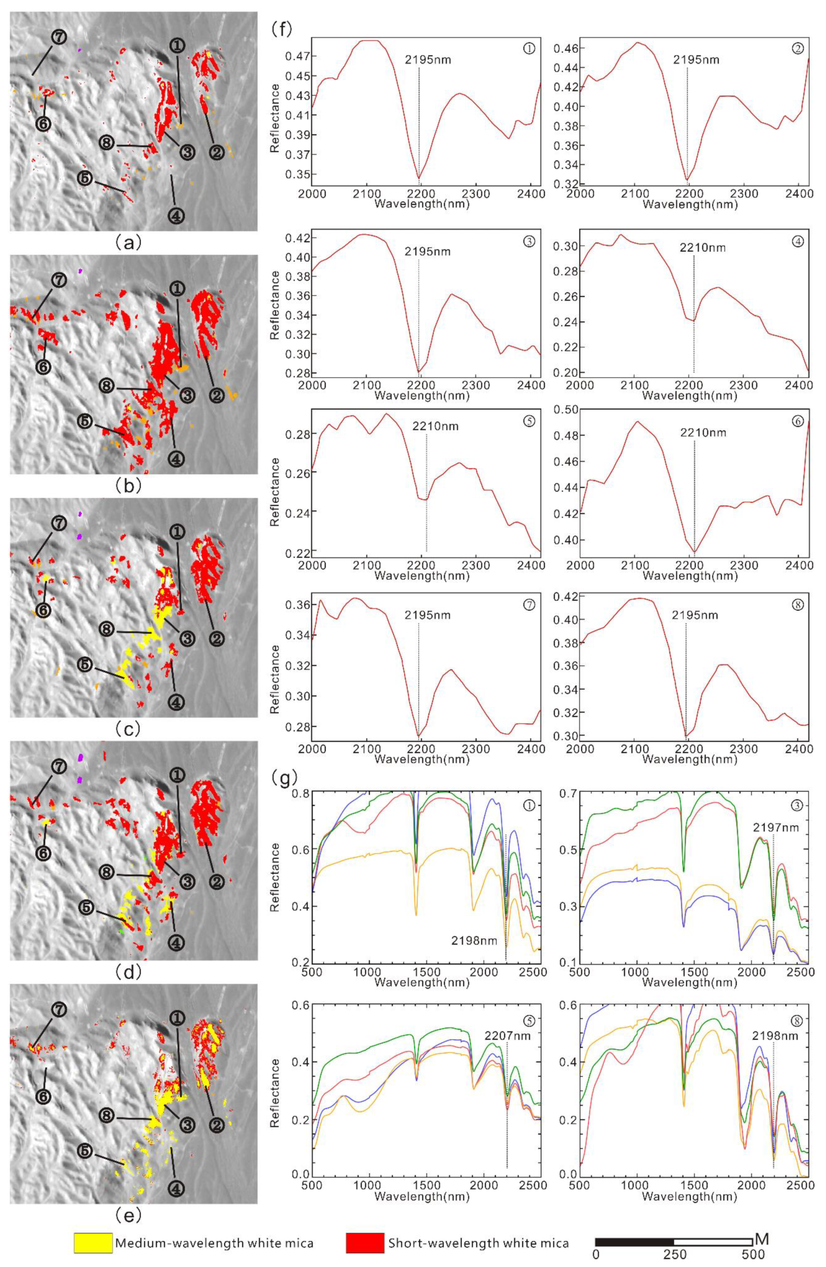
30]. The spectral features of short-wavelength white mica and medium-wavelength white mica are similar, and these two minerals also have similar spectral features to montmorillonite. Thus, their mapping accuracies have certain reference significance for model evaluation. To better verify the distinction between the two types of white mica, a section with rich white mica development in the northeastern margin of the Yangzhuang rock body was selected for spectral verification analysis, as shown in
Figure 14.
At points 1, 2, 3, 7 and 8, the MTMF method identifies medium-wavelength white mica, while the pixel spectral interpretation of these points identifies short-wavelength white mica, of which three points were confirmed by the spectral curves of rock samples collected at this point measured by an ASD spectrometer in the laboratory (
Figure 14f). Among these five points, the SVM method and the 1D CNN model identify three points accurately, the FCNN model identifies four points accurately, and the 1D and 2D CNN model identifies all points accurately. At the point 6 position, the MTMF identifies nothing, and the pixel spectral curve resembles medium-wavelength white mica. The two CNN models identify this mineral accurately, while the SVM and the FCNN both identify it as short-wavelength white mica. At points 4 and 5, the mapping results of the MTMF method identify medium-wavelength white mica, and only the mapping results of the 1D and 2D CNN model identify medium-wavelength white mica. Based on pixel spectral analyses of these two points, the Al-OH wavelength of white mica is between short-wavelength and medium-wavelength and is closer to the wavelength of medium-wavelength white mica, which may lead to certain deviations in the DNN models. This deviation may also be affected by sample noise. To ensure that the number of deep learning samples has a certain scale, some sample noise is inevitably introduced when delineating the samples. Nevertheless, in general, as shown in
Table 7, the identification effect of the CNN models for the two types of white mica is better than that of the MTMF method, the SVM method and the FCNN model, especially the 1D and 2D CNN model. According to the spectral interpretation of white mica and its surrounding pixels, the 1D and 2D CNN distinguish the boundary between short-wavelength white mica and medium-wavelength white mica more accurately than the other models.
A visual interpretation of the pixel spectrum also shows that deep learning can improve the mineral mapping of the traditional MTMF method in the Baiyanghe uranium deposit. SVM is also a good machine learning algorithm, but it lost the competition with the DNN model, which is consistent with the above model accuracy evaluation results. In general, the accuracy and identification effects of the 1D and 2D CNN are better than those of the other models, especially for distinguishing minerals with similar spectra. For this reason, the deep learning method is appealing in geology remote sensing, as many methods currently have difficulty solving this problem. Moreover, the DNN structure used in this study is not complicated but only for basic evaluation. In view of the current development speed of deep learning technology, there is much room for improvement and imagination in model structure optimization in the future.
6. Conclusions
In this paper, to investigate the practical effects of deep learning methods on airborne hyperspectral remote sensing mineral mapping, three DNN structures were designed based on the mainstream deep learning framework. Experiments were carried out in the Baiyanghe uranium deposit in Northwestern Xinjiang, China, which includes a considerable amount of altered minerals, and the results were compared with the hyperspectral remote sensing mineral mapping results of the MTMF and SVM methods. The following conclusions were reached.
(1) The feasibility and effectiveness of deep learning methods for airborne hyperspectral mineral mapping were verified. Compared with the traditional MTMF method, the DNN model improves the mineral identification accuracy. In general, the 1D and 2D CNN model has better identification effects than the other methods, which provides a reference for deep learning applications in hyperspectral remote sensing mineral mapping in future works.
(2) A CNN that combines 1D spectral features with 2D spatial features outperforms the other two DNN models in terms of the identification effect of short-wavelength and medium-wavelength white micas, which indicates that the introduction of spatial information improves the ability of CNNs to distinguish minerals with similar spectral features in airborne hyperspectral remote sensing images. Feature selection is one of the difficulties in hyperspectral remote sensing image object detection. There is no special comparative study on feature selection in this study. Therefore, the performance of the model still has room for further improvement, which is the focus of follow-up work.
In general, CNN is more suitable for image recognition than FCNN. The combination of spatial-spectral information improves the feature expression ability of hyperspectral images, which may accelerate the development of remote sensing geological mapping. In theory, a CNN model that introduces spatial information may be more effective for lithological mapping. For geological prospecting, it is often more critical to distinguish specific altered minerals in different lithologies. Therefore, it is a good idea to develop an integrated lithological and mineral mapping method in the future.
Future work will also include constructing a hyperspectral remote sensing sample library that includes more rock minerals, trying more complex DNN model structures such as 3D CNN, and performing more experimental applications and evaluations.


