Author Contributions
Conceptualisation, D.S., J.C.-F., A.L. and A.C.T.; methodology, D.S., J.C.-F., A.L. and A.C.T.; software, D.S. and J.C.-F.; formal analysis D.S., J.C.-F., M.B. and A.M.; investigation, D.S., J.C.-F., A.L., A.C.T., M.B. and A.M.; resources A.L. and A.M.; data curation, D.S. and J.C.-F.; writing—original draft preparation, D.S.; writing—review and editing, all remaining authors; visualisation, D.S. and J.C.-F.; supervision, A.C.T., J.C.-F. and A.L.; project administration D.S., A.C.T., J.C.-F., A.L. and A.M.; funding acquisition, A.M. and A.L. All authors have read and agreed to the published version of the manuscript.
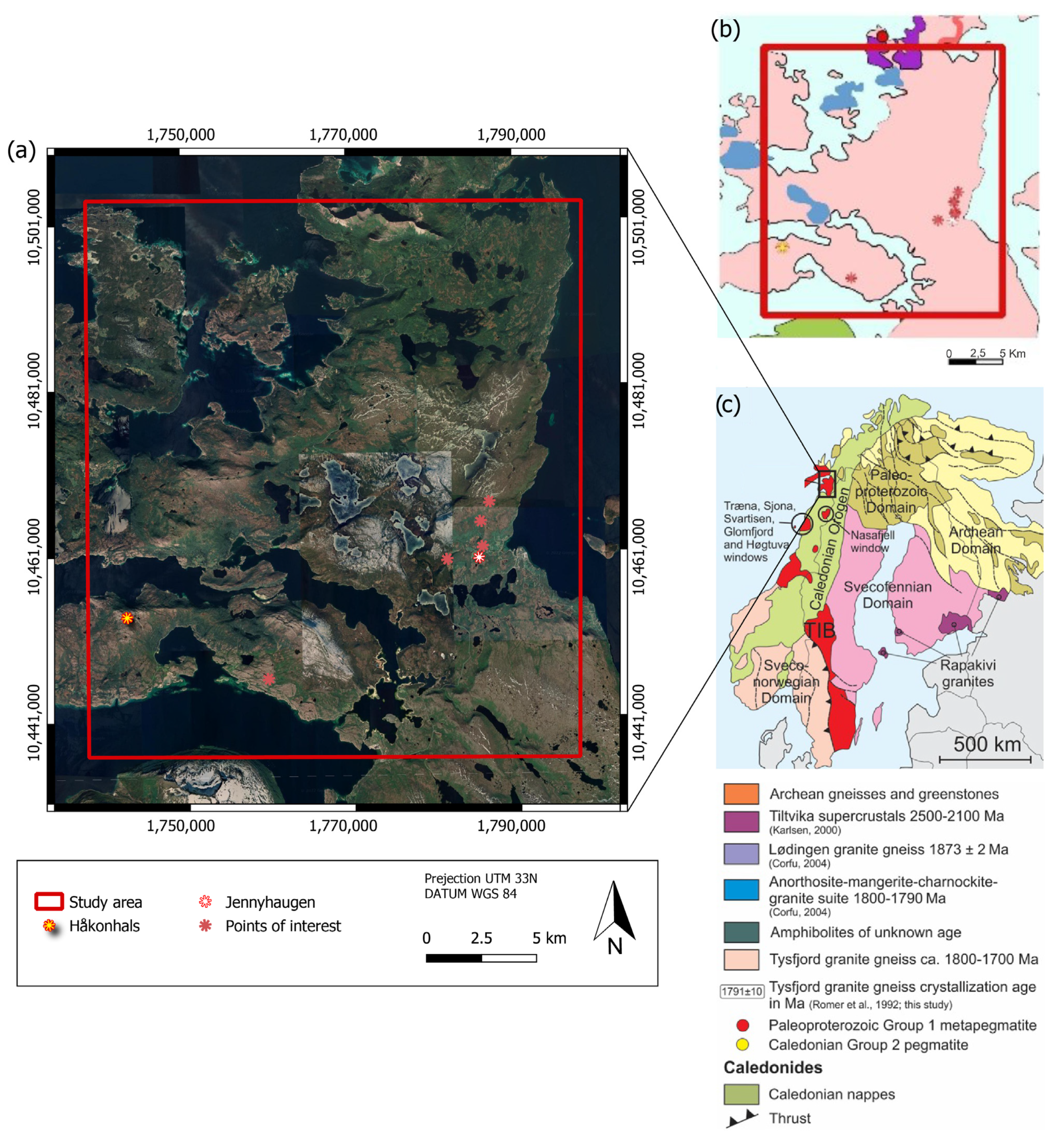
Figure 1.
Location of the study area. (
a) Overview image of the Tysfjord district where the study area is framed by the red square. The Håkonhals pegmatite is marked with a yellow star, Jennyhaugen mine with a white star, and other pegmatites with red stars. (
b) Simplified geologic map. (
c) Detailed geological map and location of the study area in Norway. TIB: Trans-Scandinavian Igneous Belt. Adapted with permission from Müller et al. [
4,
5].
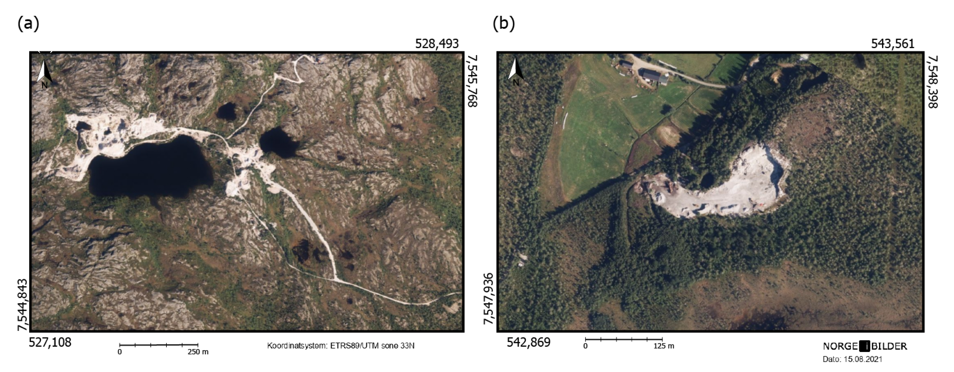
Figure 2.
High-resolution aerial photographs of the (
a) Håkonhals and (
b) Jennyhaugen mines that were used as target areas in this study. Adapted with permission from Norge I bilder [
23].
Figure 2.
High-resolution aerial photographs of the (
a) Håkonhals and (
b) Jennyhaugen mines that were used as target areas in this study. Adapted with permission from Norge I bilder [
23].
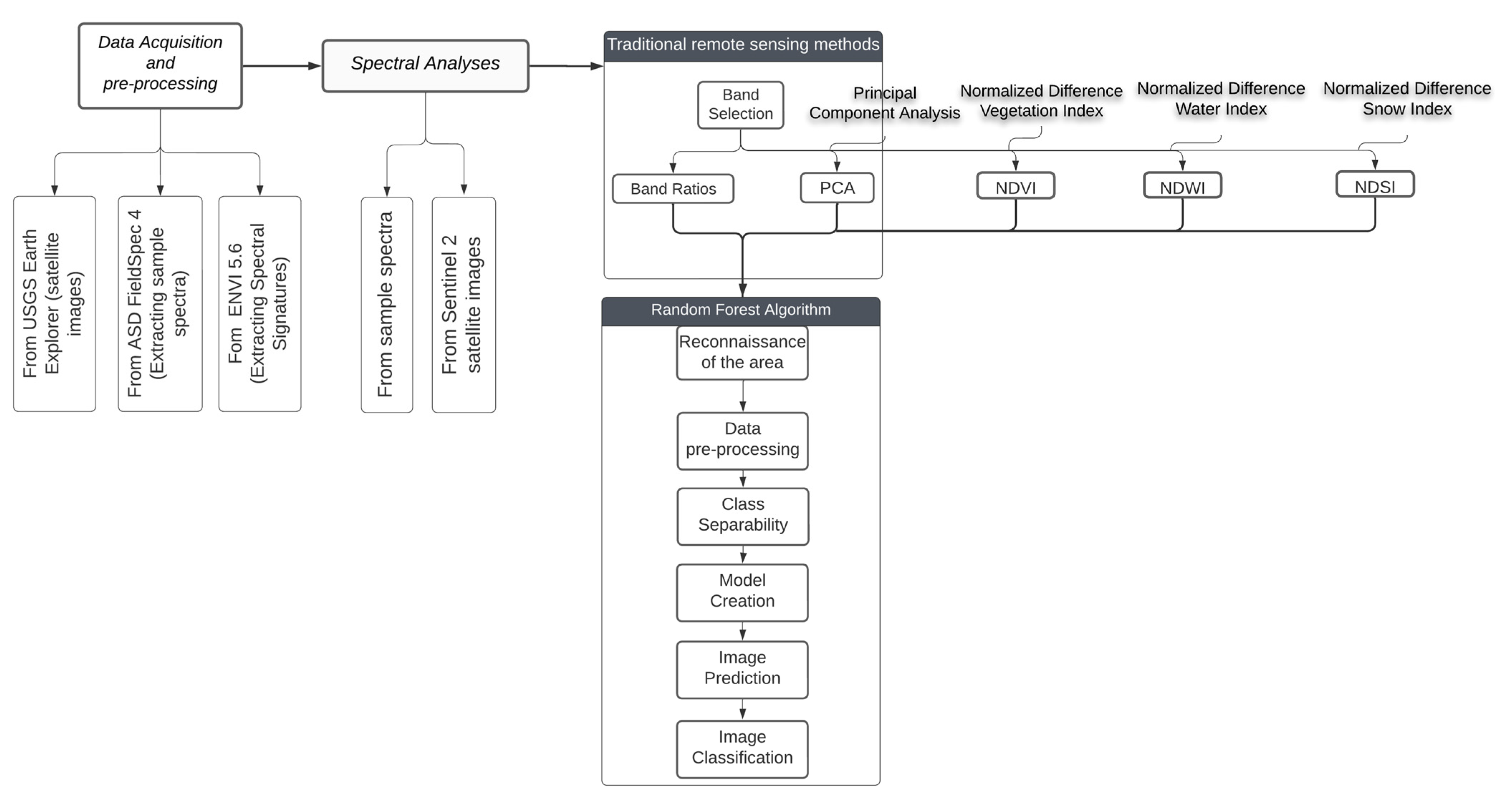
Figure 3.
Workflow of the applied methodology to select and adapt the traditional remote sensing methods.
Figure 3.
Workflow of the applied methodology to select and adapt the traditional remote sensing methods.
Figure 4.
Overall comparison between (a) raw and (b) continuum-removed spectra of the Håkonhals mine.
Figure 4.
Overall comparison between (a) raw and (b) continuum-removed spectra of the Håkonhals mine.
Figure 5.
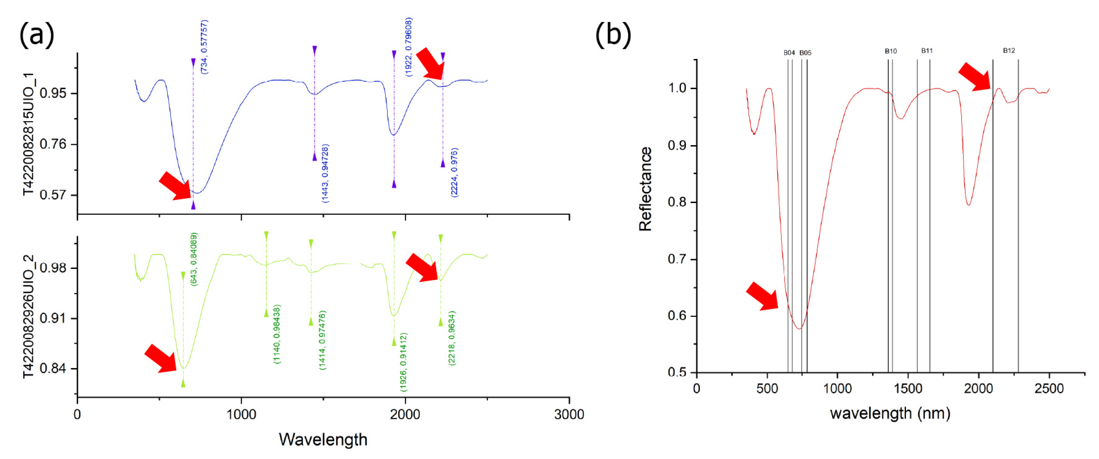
Spectra of amazonite samples from Tysfjord. (a) It is possible to see—indicated by red arrows—the main absorptions of the spectra collected in the laboratory. (b) Comparison of the absorption and reflectance features—indicated by red arrows—with the spectral range of the Sentinel 2 satellite bands.
Figure 5.
Spectra of amazonite samples from Tysfjord. (a) It is possible to see—indicated by red arrows—the main absorptions of the spectra collected in the laboratory. (b) Comparison of the absorption and reflectance features—indicated by red arrows—with the spectral range of the Sentinel 2 satellite bands.
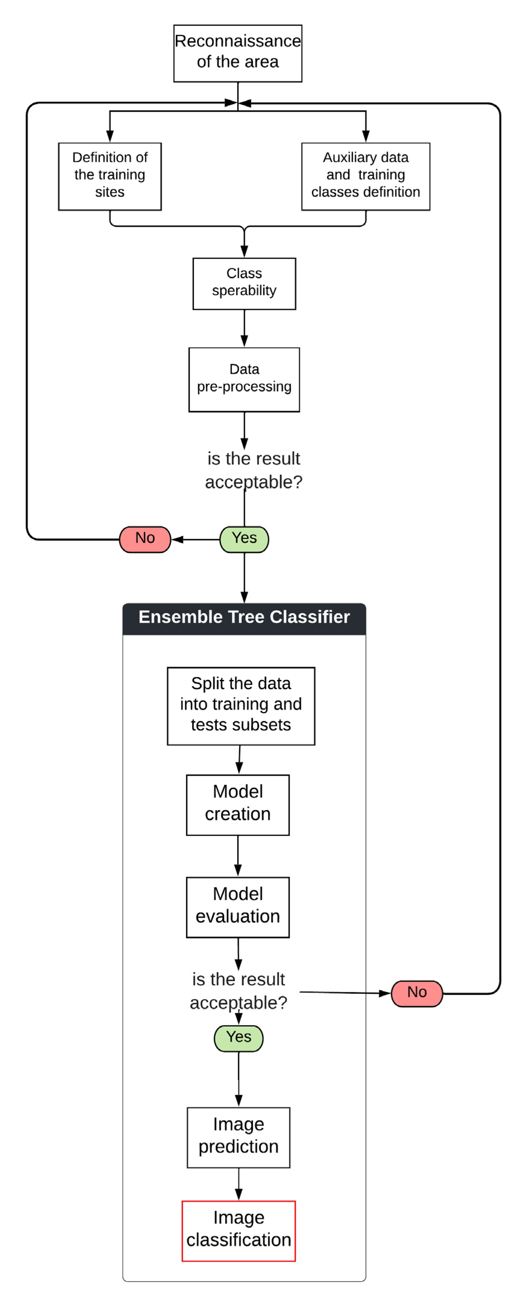
Figure 6.
Workflow showing the step-by-step method applied to the RF algorithm.
Figure 6.
Workflow showing the step-by-step method applied to the RF algorithm.
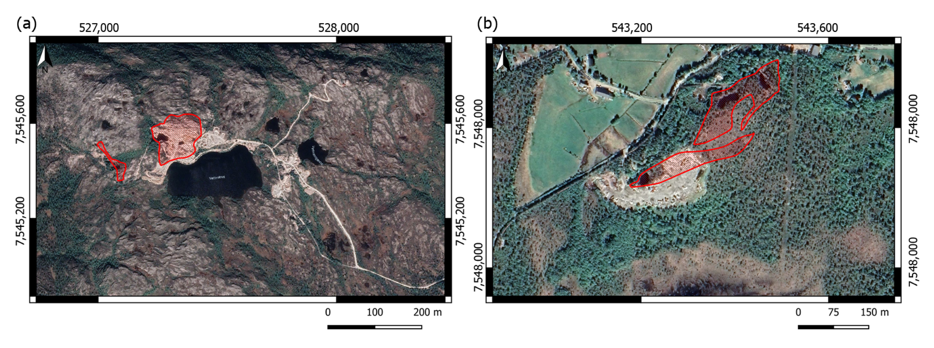
Figure 7.
Outcrop of pegmatites identified in red polygons. (a) Pegmatite outcrop at Håkonhals. (b) Pegmatite outcrop at Jennyhaugen. The area outside the pegmatite outcrop and within the mining areas may also contain pegmatitic materials.
Figure 7.
Outcrop of pegmatites identified in red polygons. (a) Pegmatite outcrop at Håkonhals. (b) Pegmatite outcrop at Jennyhaugen. The area outside the pegmatite outcrop and within the mining areas may also contain pegmatitic materials.
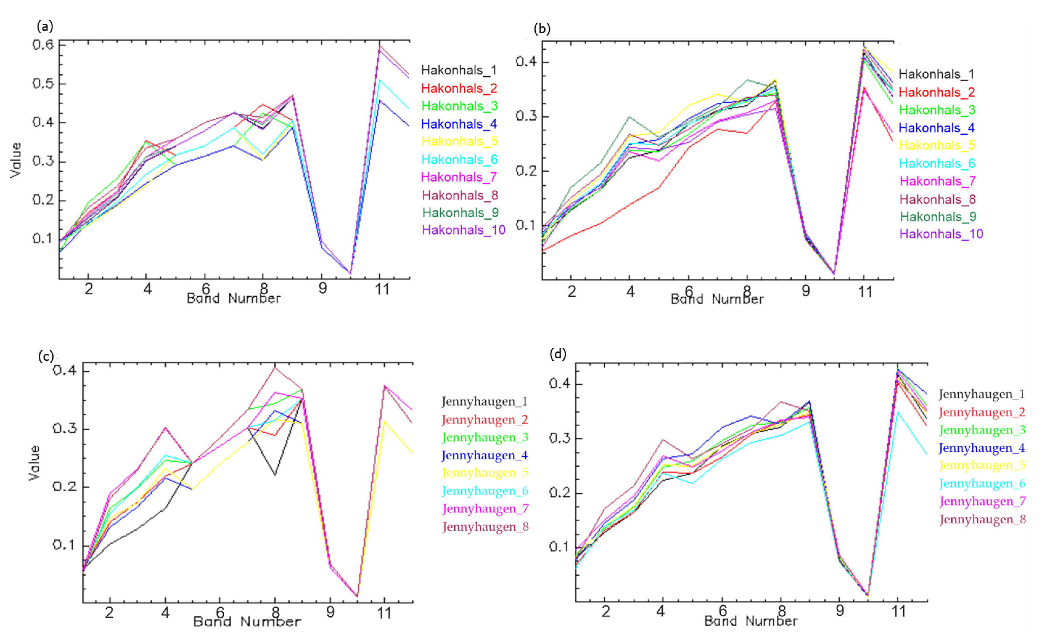
Figure 8.
Sentinel 2 spectral behaviour pure pegmatite spectra (unaveraged) and mining spectra derived from averaging. Håkonhals and Jennyhaugen mines. (a) Håkonhals pure spectra. (b) Håkonhals mining spectra. (c) Jennyhaugen pure spectra. (d) Jennyhaugen mining spectra.
Figure 8.
Sentinel 2 spectral behaviour pure pegmatite spectra (unaveraged) and mining spectra derived from averaging. Håkonhals and Jennyhaugen mines. (a) Håkonhals pure spectra. (b) Håkonhals mining spectra. (c) Jennyhaugen pure spectra. (d) Jennyhaugen mining spectra.
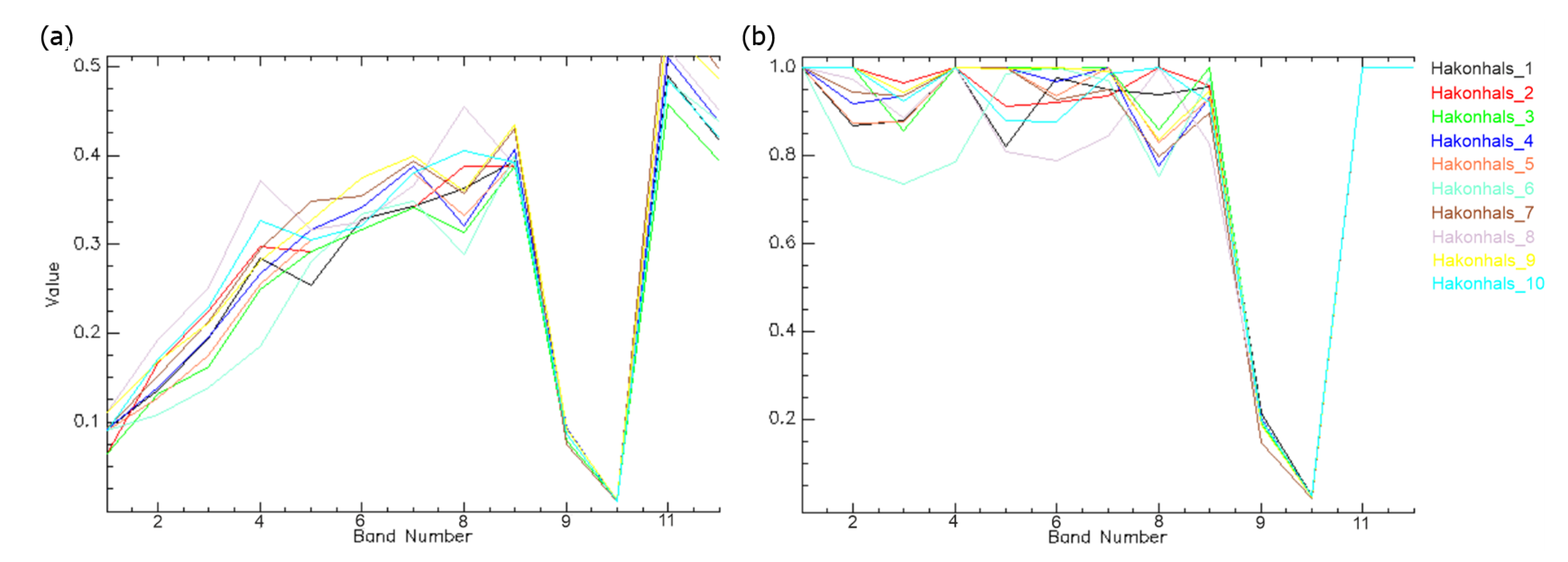
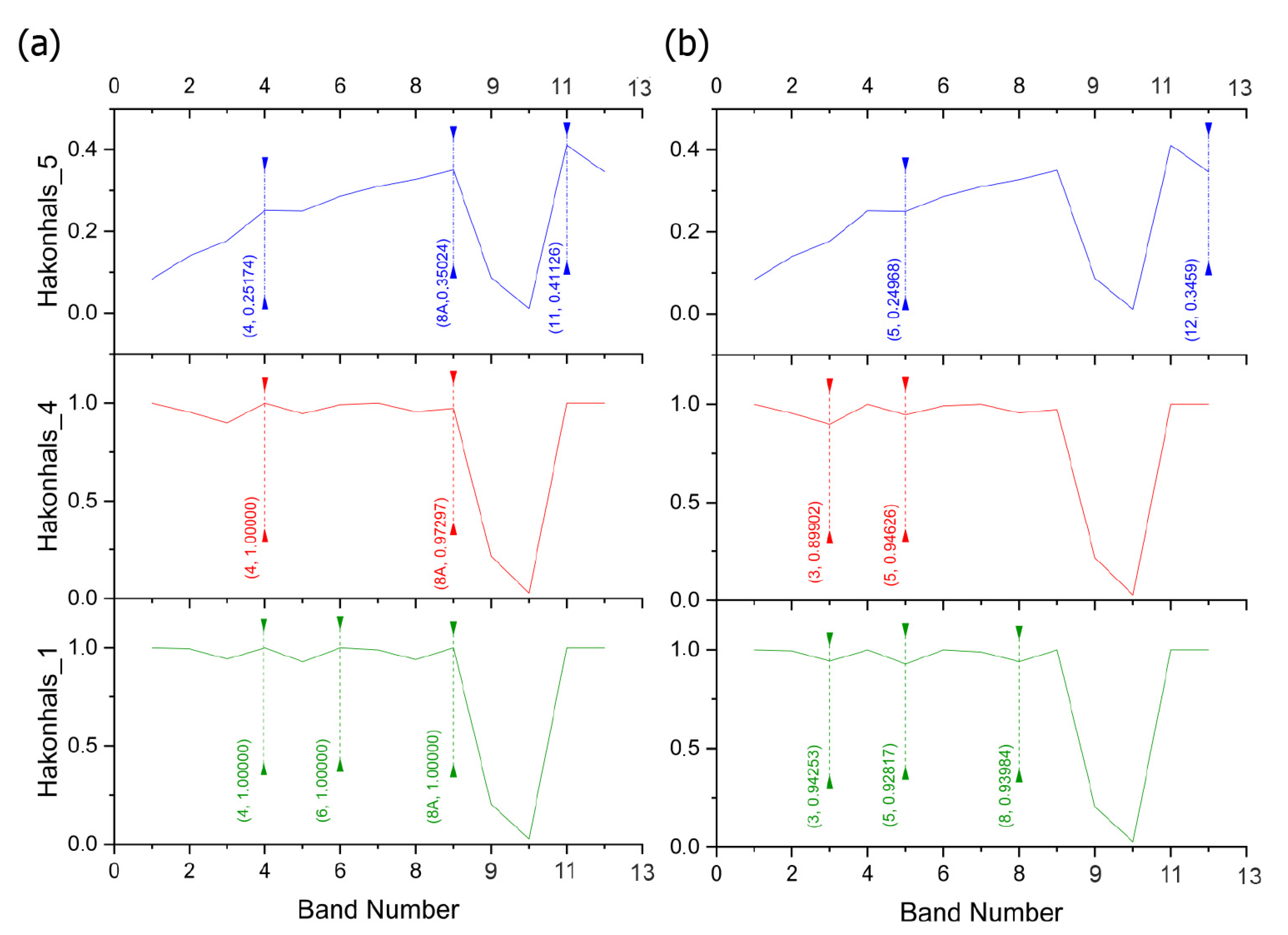
Figure 9.
Sentinel 2 spectral behaviour from Håkonhals mine (mining spectra). (a) Bands in absorption features. (b) Bands in reflectance peaks. For each spectrum, in either absorption or reflectance regions, is presented, between brackets, the number of the Sentinel 2 bands, and the respective reflectance value.
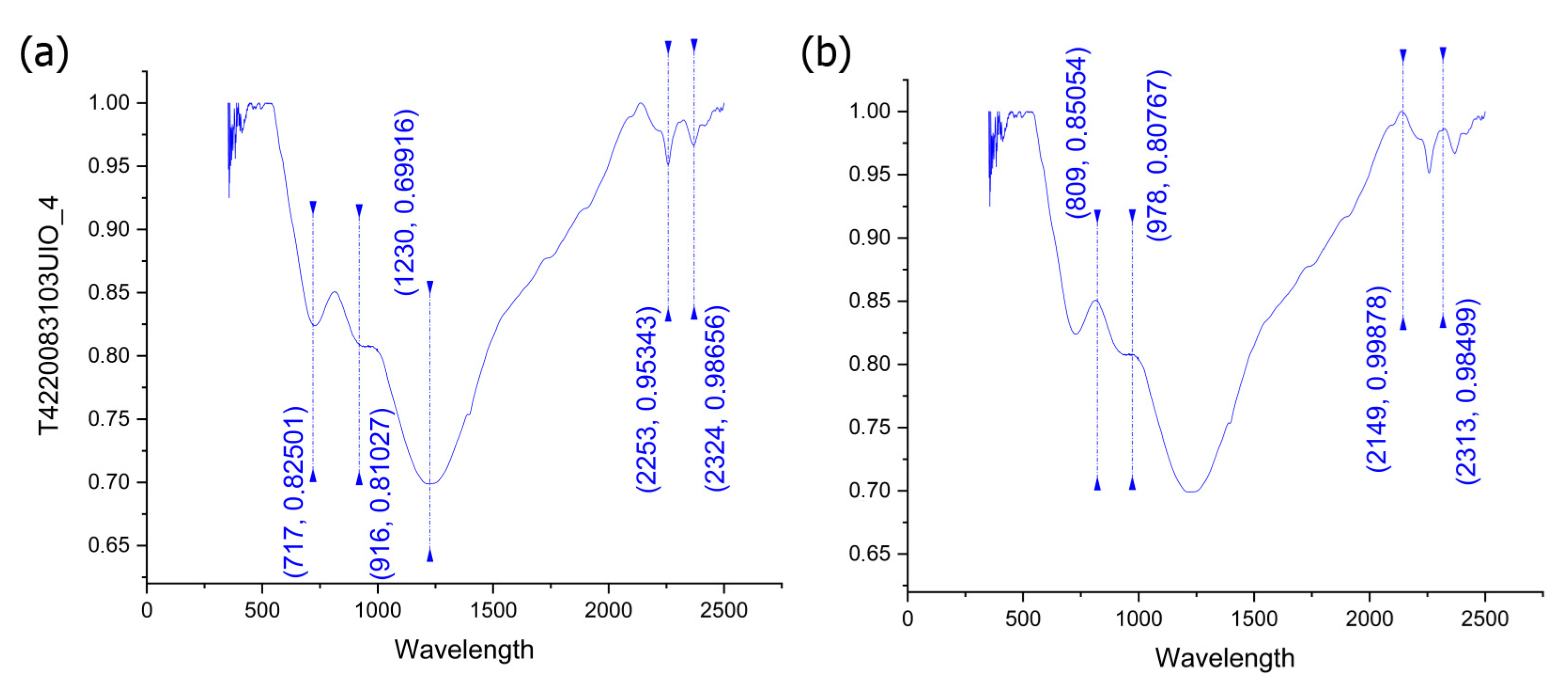
Figure 10.
Absorption and reflectance peaks from spectra collected from samples of Tysfjord plagioclases. (a) Main absorption peaks (minimum). (b) Main reflectance peaks.
Figure 10.
Absorption and reflectance peaks from spectra collected from samples of Tysfjord plagioclases. (a) Main absorption peaks (minimum). (b) Main reflectance peaks.
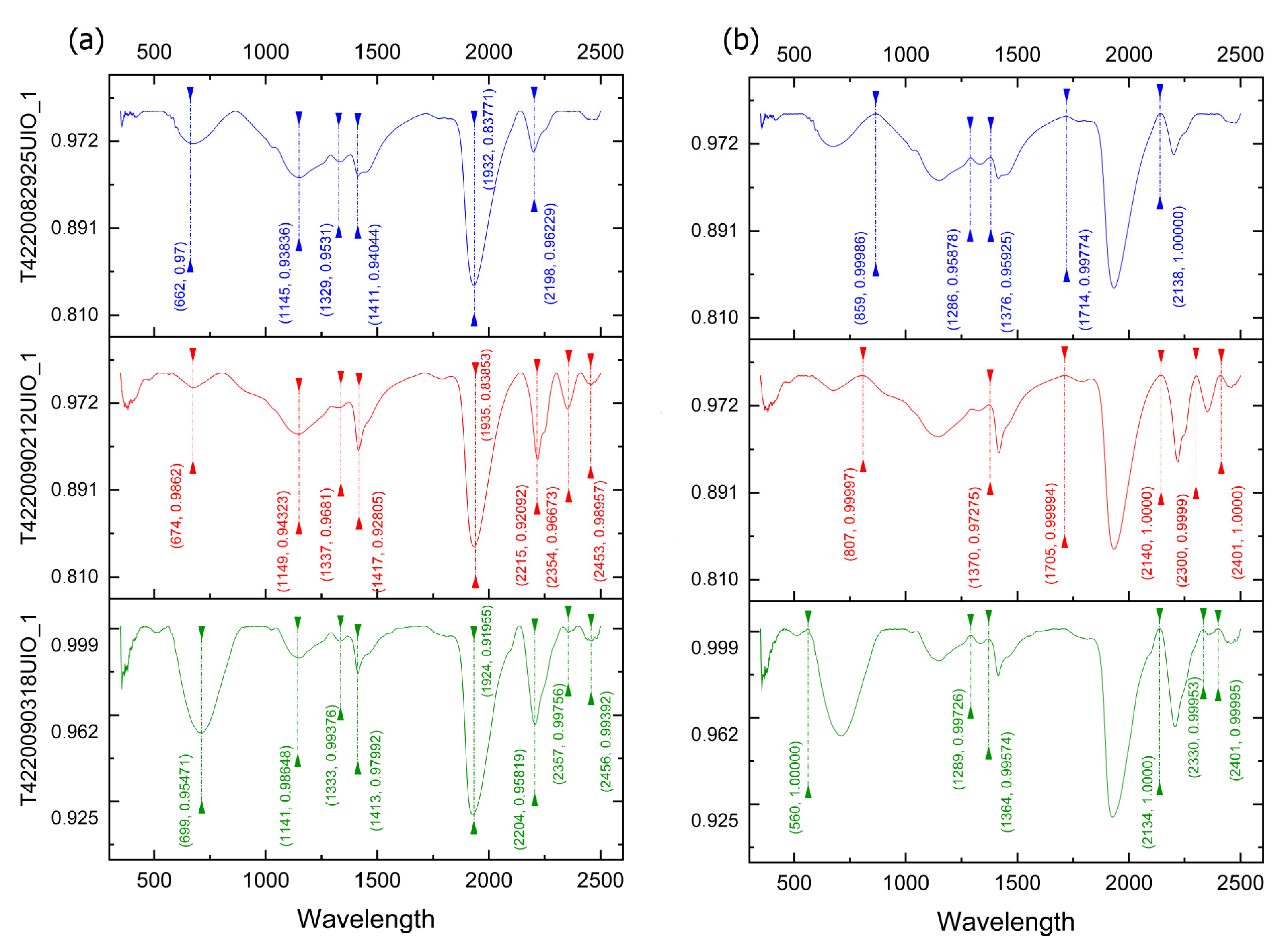
Figure 11.
Absorption and reflectance peaks from spectra collected from samples of Tysfjord K-feldspar. (a) Main absorption peaks (minimum). (b) Main reflectance peaks.
Figure 11.
Absorption and reflectance peaks from spectra collected from samples of Tysfjord K-feldspar. (a) Main absorption peaks (minimum). (b) Main reflectance peaks.
Figure 12.
Absorption and reflectance peaks from spectra collected from samples of Tysfjord biotite. (a) Main absorption peaks (minimum). (b) Main reflectance peaks.
Figure 12.
Absorption and reflectance peaks from spectra collected from samples of Tysfjord biotite. (a) Main absorption peaks (minimum). (b) Main reflectance peaks.
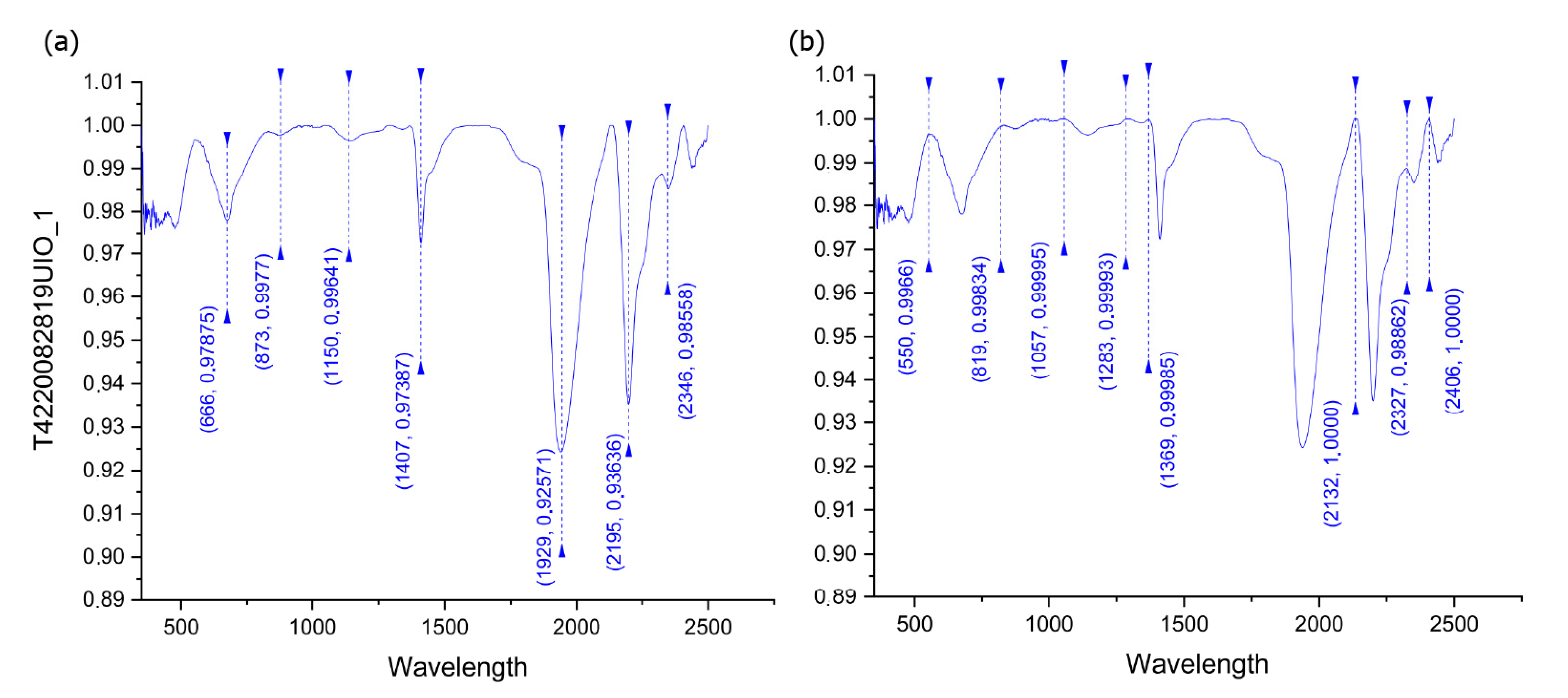
Figure 13.
Absorption and reflectance peaks from spectra collected from pegmatite quartz samples of Tysfjord. (a) Main absorption peaks (minimum). (b) Main reflectance peaks.
Figure 13.
Absorption and reflectance peaks from spectra collected from pegmatite quartz samples of Tysfjord. (a) Main absorption peaks (minimum). (b) Main reflectance peaks.
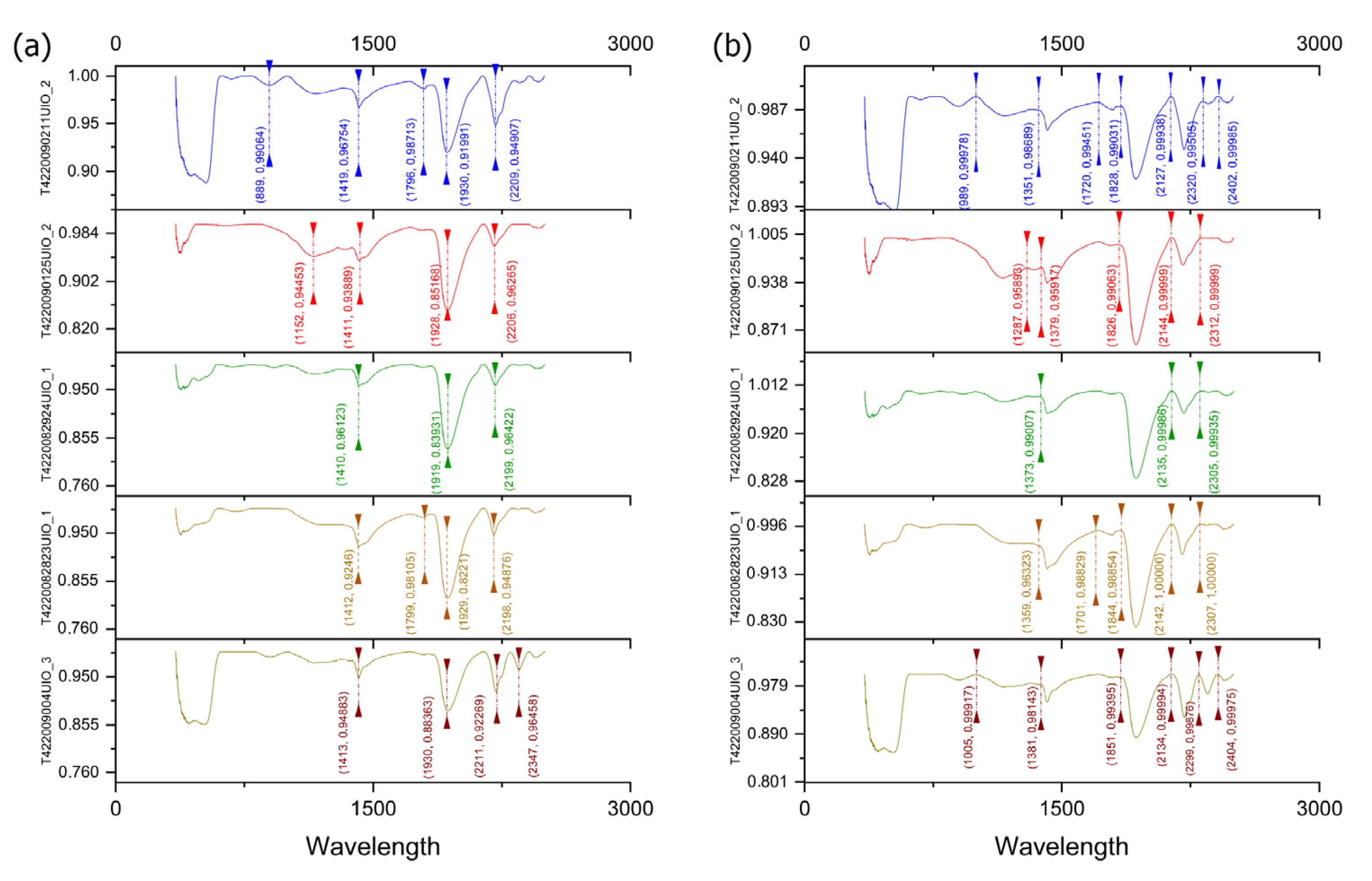
Figure 14.
Absorption and reflectance peaks from spectra collected from samples of Tysfjord granite. (a) Main absorption peaks (minimum). (b) Main reflectance peaks.
Figure 14.
Absorption and reflectance peaks from spectra collected from samples of Tysfjord granite. (a) Main absorption peaks (minimum). (b) Main reflectance peaks.
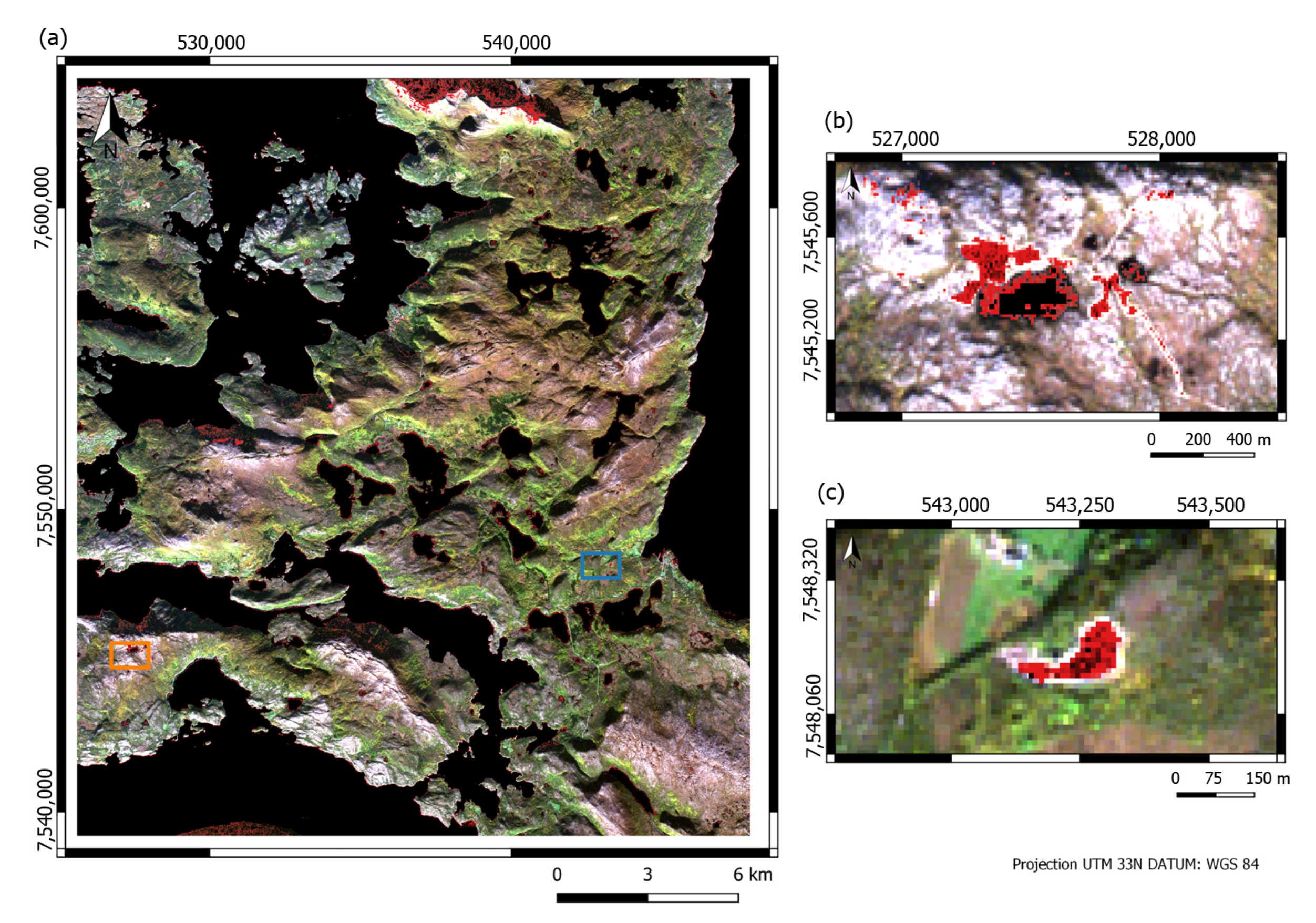
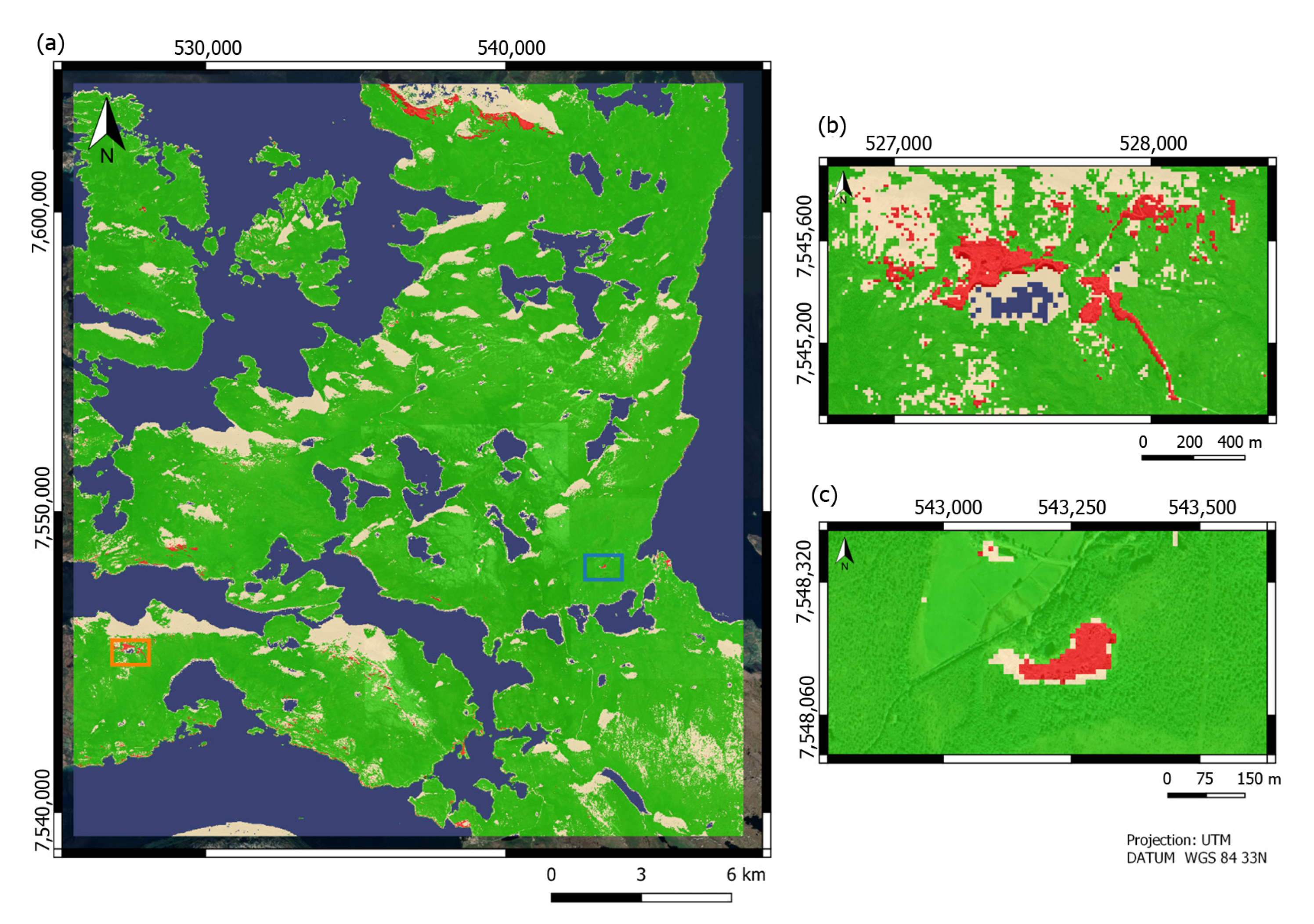
Figure 15.
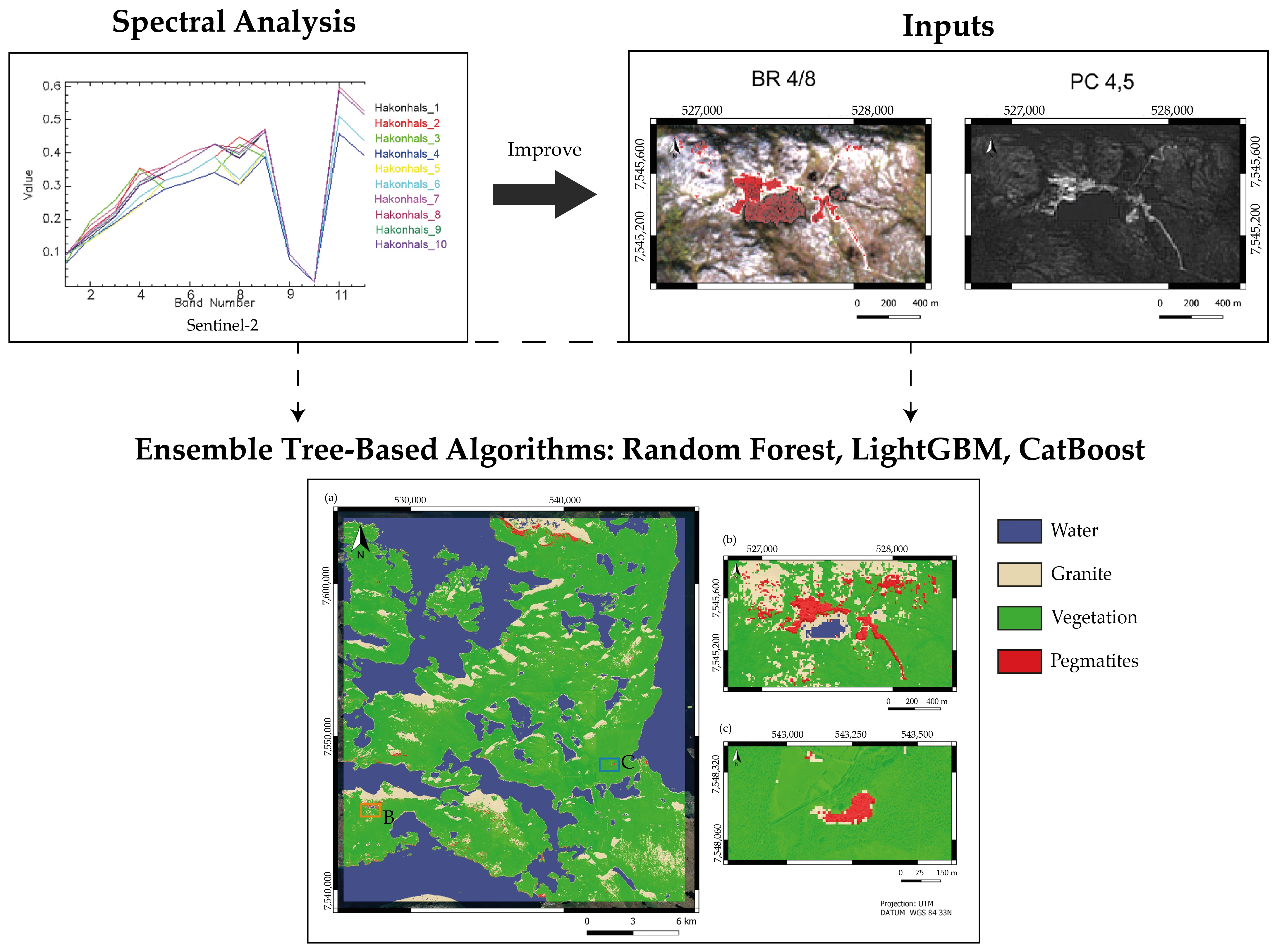
Result for BR 4/8. Pixels higher than 0.70 are represented in red colour. (a) Overview of the study area where Håkonhals mine is highlighted by the orange rectangle and Jennyhaugen mine by the blue rectangle. (b) Håkonhals mine in focus. (c) Jennyhaugen mine in focus.
Figure 15.
Result for BR 4/8. Pixels higher than 0.70 are represented in red colour. (a) Overview of the study area where Håkonhals mine is highlighted by the orange rectangle and Jennyhaugen mine by the blue rectangle. (b) Håkonhals mine in focus. (c) Jennyhaugen mine in focus.
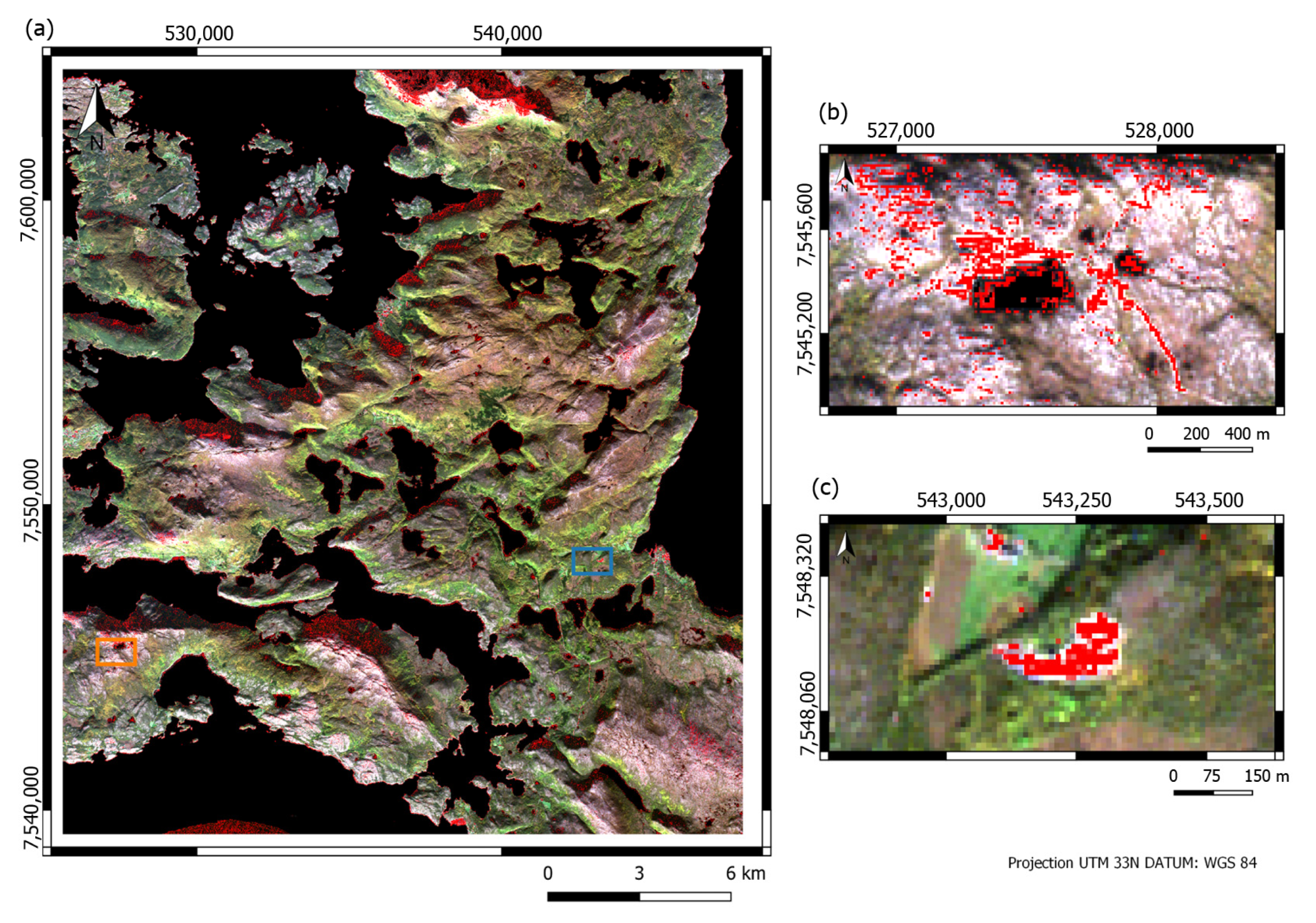
Figure 16.
Result for BR 4/5. (a) Overview of the study area where Håkonhals mine is highlighted by the orange rectangle and Jennyhaugen mine by the blue rectangle. (b) Håkonhals mine in focus. Here it can be seen that this BR has also highlighted many granite pixels with elevated values. (c) Jennyhaugen mine in focus.
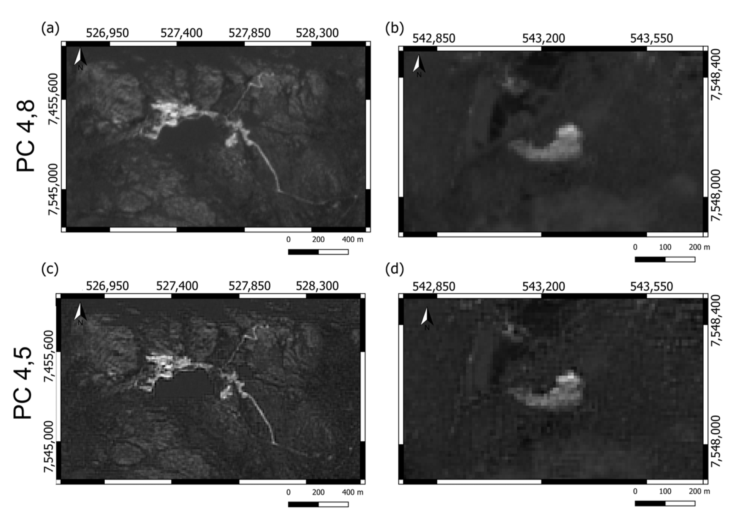
Figure 17.
Comparison of PCA results of bands 4 and 5 and 4 and 8. (a) Håkonhals mine in focus for PCA 4, 8. (b) Jennyhaugen mine in focus for PCA 4 And 8. (c) Håkonhals mine in focus for PCA 4, 5. (d) Jennyhaugen mine in focus for PCA 4, 5.
Figure 17.
Comparison of PCA results of bands 4 and 5 and 4 and 8. (a) Håkonhals mine in focus for PCA 4, 8. (b) Jennyhaugen mine in focus for PCA 4 And 8. (c) Håkonhals mine in focus for PCA 4, 5. (d) Jennyhaugen mine in focus for PCA 4, 5.
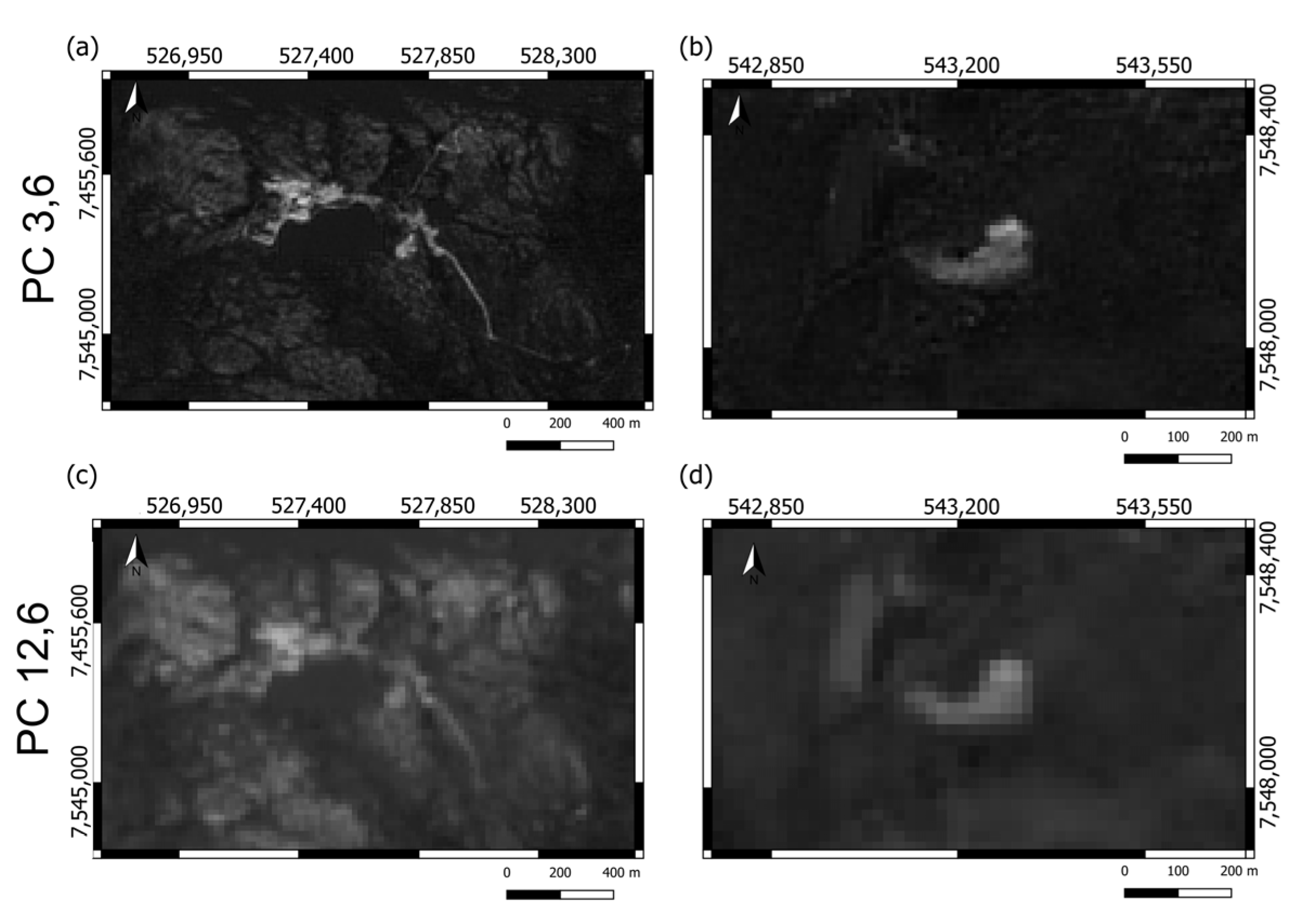
Figure 18.
Comparison of PCA results of bands 3, 6 and 12, 6. (a) Håkonhals mine in focus for PCA 3, 6. (b) Jennyhaugen mine in focus for PCA 3, 6. (c) Håkonhals mine in focus for PCA 12, 6. (d) Jennyhaugen mine in focus for PCA 12, 6.
Figure 18.
Comparison of PCA results of bands 3, 6 and 12, 6. (a) Håkonhals mine in focus for PCA 3, 6. (b) Jennyhaugen mine in focus for PCA 3, 6. (c) Håkonhals mine in focus for PCA 12, 6. (d) Jennyhaugen mine in focus for PCA 12, 6.
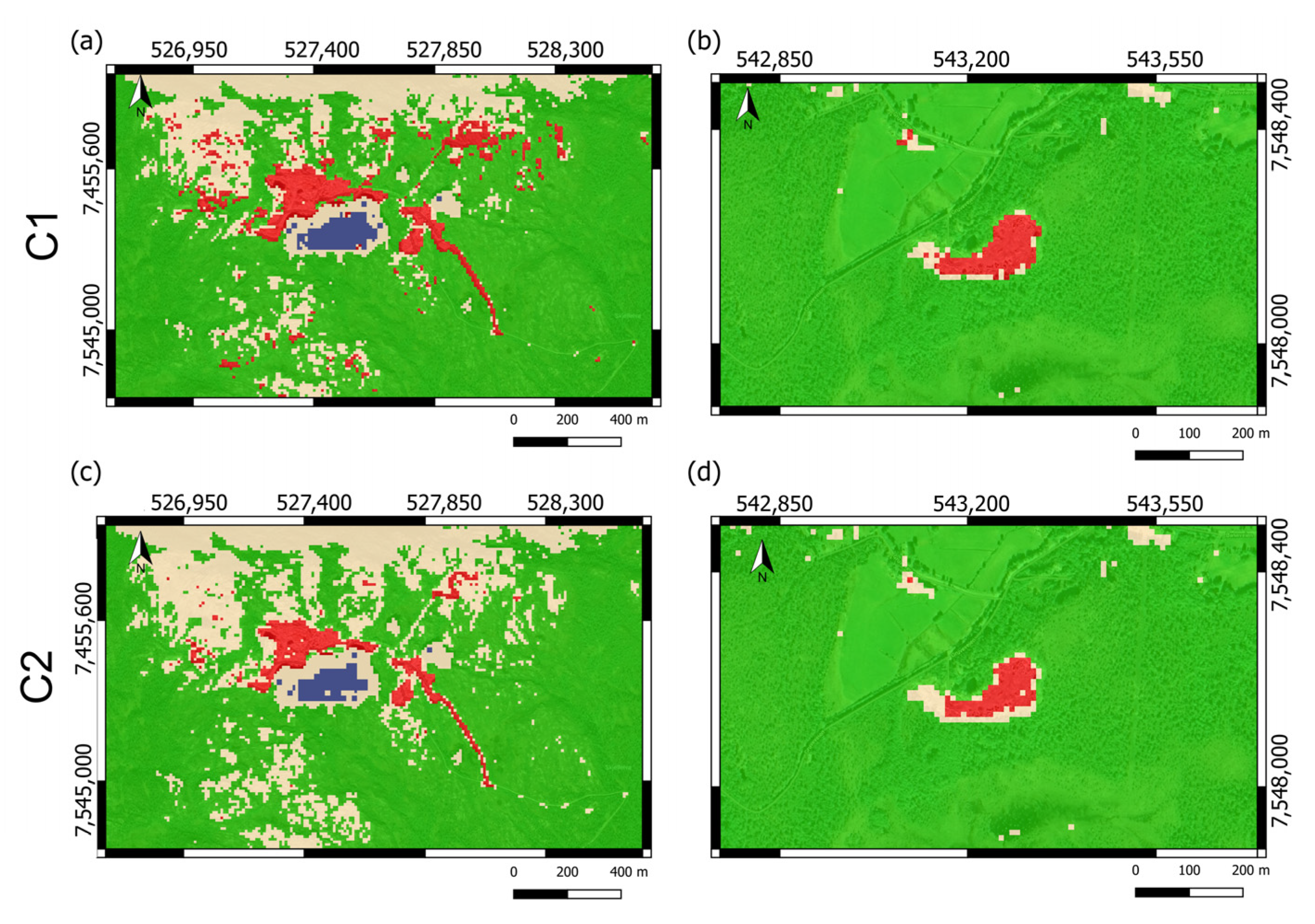
Figure 19.
RF classifier for C1 and C2 models. Pegmatites are classified as red colour, granite as beige, water as blue, and vegetation as green (a) C1 model classification for Håkonhals mine. (b) C1 model classification for Jennyhaugen mine. (c) C2 model classification for Håkonhals mine. (d) C2 model classification for Jennyhaugen mine.
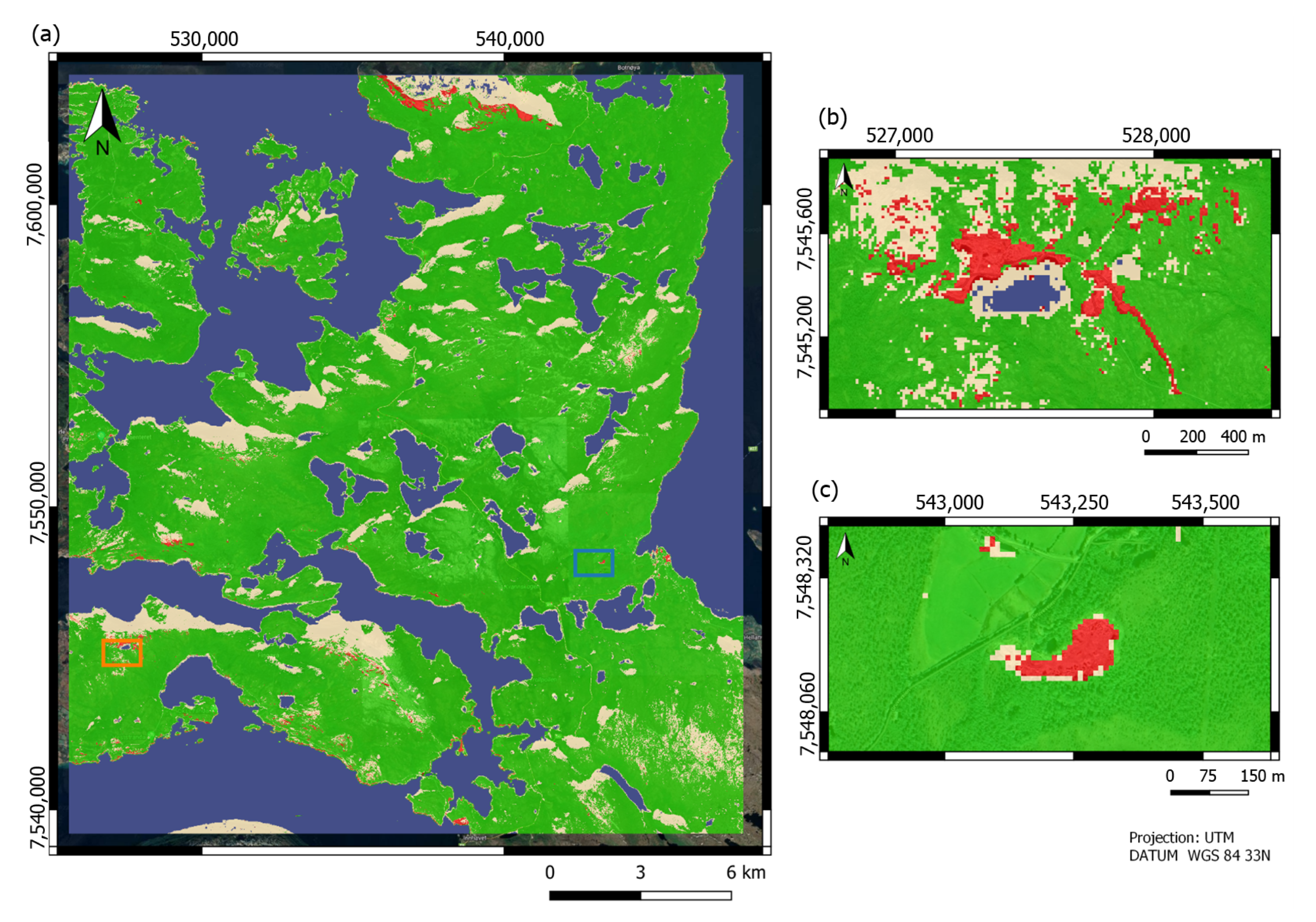
Figure 20.
RF classifier. Pegmatites are classified as red colour, granite as beige, water as blue, and vegetation as green. (a) Overview of the study area where Håkonhals mine is highlighted by the orange rectangle and Jennyhaugen mine by the blue rectangle. (b) Håkonhals mine in focus. (c) Jennyhaugen mine in focus.
Figure 21.
LGB classifier. Pegmatites are classified as red colour, granite as beige, water as blue, and vegetation as green (a) Overview of the study area where Håkonhals mine is highlighted by the orange rectangle and Jennyhaugen mine by the blue rectangle. (b) Håkonhals mine in focus. (c) Jennyhaugen mine in focus.
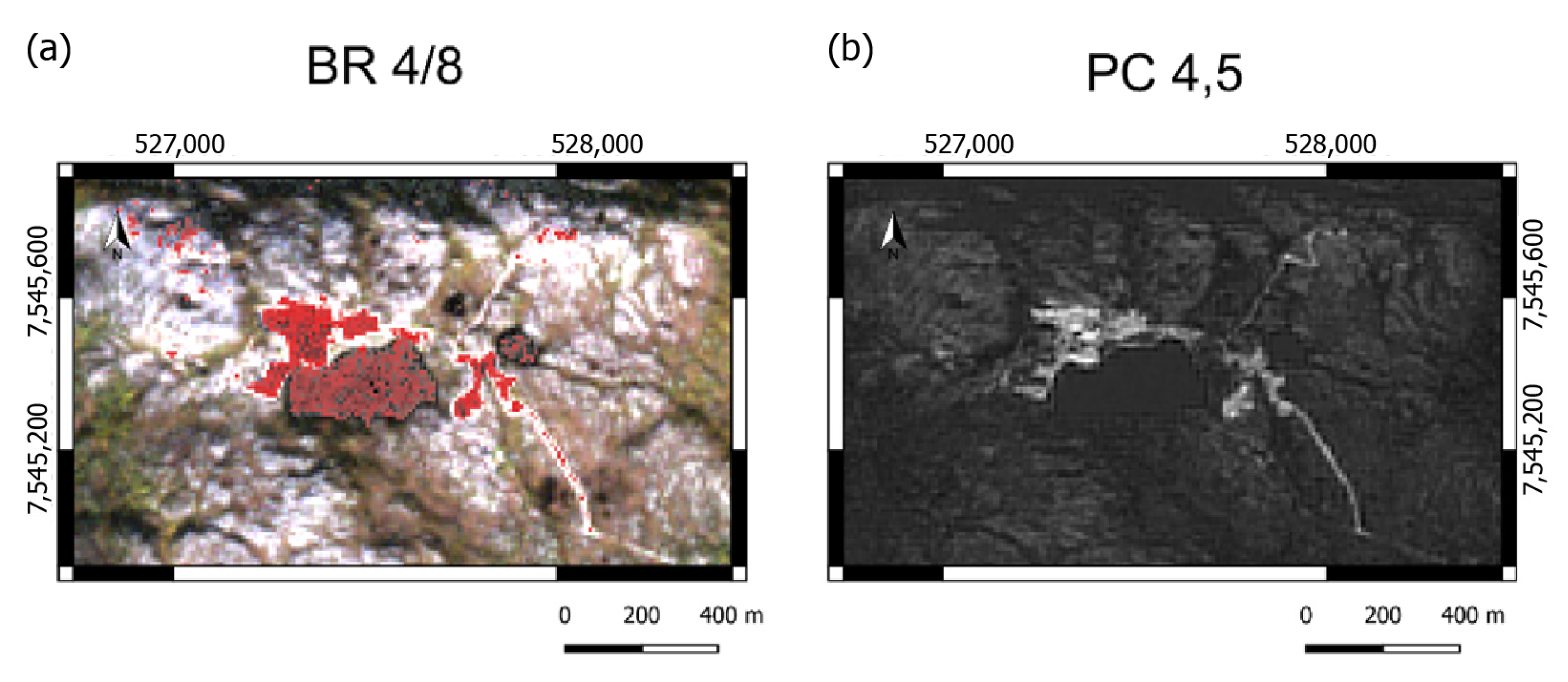
Figure 22.
Comparison of the best BR and PCA results with the Håkonhals mine in focus. (a) BR 4/8. It is possible to see that the ratio also highlights water bodies and granite. (b) PCA of bands 4, 5. Note that it identifies the target area perfectly with no signal confusion with water or granite.
Figure 22.
Comparison of the best BR and PCA results with the Håkonhals mine in focus. (a) BR 4/8. It is possible to see that the ratio also highlights water bodies and granite. (b) PCA of bands 4, 5. Note that it identifies the target area perfectly with no signal confusion with water or granite.
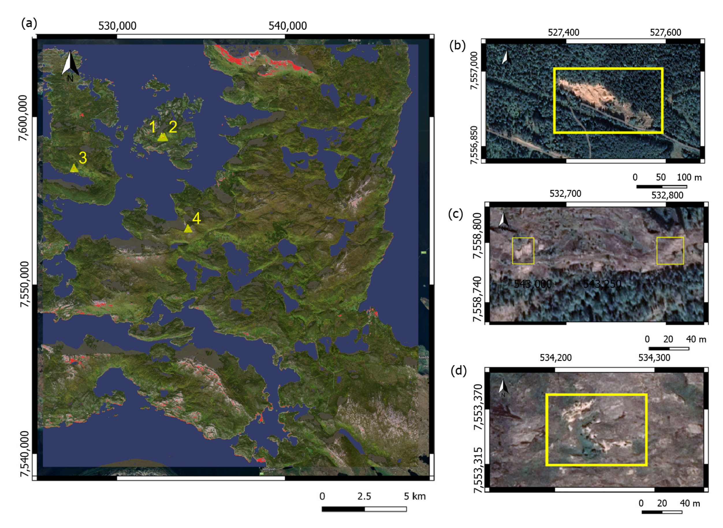
Figure 23.
Points of interest for exploration. (a) Overview of the study area where the points of interest were identified by the yellow rectangle. (b) Points 1 and 2 in focus. (c) Point 3 in focus. (d) Point 4 in focus.
Figure 23.
Points of interest for exploration. (a) Overview of the study area where the points of interest were identified by the yellow rectangle. (b) Points 1 and 2 in focus. (c) Point 3 in focus. (d) Point 4 in focus.
Table 1.
BR developed through spectral analysis of spectra collected in the laboratory. The spectra were organised according to mineral samples.
Table 1.
BR developed through spectral analysis of spectra collected in the laboratory. The spectra were organised according to mineral samples.
| Granite | Plagioclase | Biotite | Quartz |
|---|
| 3/6 | 8A/4 | 8/5 | 3/4 |
| 12/6 | 8A/11 | xx | 3/12 |
| 8/6 | xx | xx | 8/12 |
Table 2.
BR developed through spectral analysis of spectra extracted from Sentinel 2 bands. The spectra were organised according to reflectance bands.
Table 2.
BR developed through spectral analysis of spectra extracted from Sentinel 2 bands. The spectra were organised according to reflectance bands.
| Band 4 | Band 6 | Band 7 | Band 8A |
|---|
| 4/3 | 6/3 | 7/3 | 8A/3 |
| 4/5 | 6/5 | 7/5 | 8A/5 |
| 4/8 | 6/8 | 7/8 | 8A/8 |
Table 3.
PCA on two bands developed through spectral analysis of spectra collected in the laboratory and extracted from Sentinel 2 bands.
Table 3.
PCA on two bands developed through spectral analysis of spectra collected in the laboratory and extracted from Sentinel 2 bands.
| PC2 Laboratory Spectra | PC2 Extracted from Sentinel 2 Bands |
|---|
| 3 and 6 | 4 and 8 |
| 12 and 6 | 4 and 5 |
Table 4.
Scores for RF model.
Table 4.
Scores for RF model.
| Kappa Statistics: C1 = 0.95/C2 = 0.96 |
|---|
| Mean Cross-Validation Score (Accuracy): C1 = 0.96/C2 = 0.97 |
|---|
| | Precision | Recall | F1 Score |
|---|
| | C1 | C2 | C1 | C2 | C1 | C2 |
| Granite | 0.95 | 0.92 | 0.90 | 0.97 | 0.93 | 0.95 |
| Pegmatite | 0.95 | 0.91 | 0.97 | 1.00 | 0.96 | 0.95 |
| Vegetation | 0.98 | 1.00 | 0.99 | 1.00 | 0.99 | 1.00 |
| Water | 1.00 | 1.00 | 1.00 | 0.97 | 1.00 | 0.98 |
Table 5.
C1 model confusion matrix.
Table 5.
C1 model confusion matrix.
| Predicted |
|---|
| | Granite | Pegmatite | Vegetation | Water |
|---|
| Granite | 37 | 2 | 3 | 0 |
| Pegmatite | 2 | 58 | 0 | 0 |
| Vegetation | 0 | 1 | 99 | 0 |
| Water | 0 | 0 | 0 | 39 |
Table 6.
Signature separability for training classes.
Table 6.
Signature separability for training classes.
| | Pegmatite | Granite | Water | Vegetation |
|---|
| Pegmatite | | | | |
| Granite | 1.953983 | | | |
| Water | 2.000000 | 1.999965 | | |
| Vegetation | 1.993627 | 1.964088 | 1.999998 | |
Table 7.
Importance of inputs in image classification, measured in percentage.
Table 7.
Importance of inputs in image classification, measured in percentage.
| Input | Importance C1 | Importance LightGBM | Importance Catboost |
|---|
| Band 04 | 16.46 | 9.4 | 13.25 |
| Band 06 | 12.24 | 13.18 | 12.27 |
| Band 07 | 15.06 | 11.77 | 11.35 |
| Band 8A | 5.22 | 10.93 | 11.54 |
| PCA 4, 5 | 1.20 | 5.6 | 4.8 |
| PCA 4, 8 | 13.35 | 11.79 | 11.24 |
| BR_4/5 | 8.03 | 4.3 | 3.8 |
| BR_4/8 | 8.53 | 18.57 | 14.69 |
| NDVI | 19.87 | 14.25 | 16.95 |


 ,
, 


