Article

Bird-Borne Samplers for Monitoring CO2 and Atmospheric Physical Parameters

by
Annalisa Di Bernardino
1,*,
Valeria Jennings
2,3 and
Giacomo Dell’Omo
2
1
Department of Physics, University of Rome “La Sapienza”, 00185 Rome, Italy
2
Ornis Italica, 00199 Rome, Italy
3
Department of Ecological and Biological Sciences, University of Tuscia, 01100 Viterbo, Italy
*
Author to whom correspondence should be addressed.
Remote Sens. 2022, 14(19), 4876; https://doi.org/10.3390/rs14194876
Submission received: 30 August 2022 / Revised: 21 September 2022 / Accepted: 27 September 2022 / Published: 29 September 2022
(This article belongs to the Section Urban Remote Sensing)

Abstract

:
Air quality monitoring in cities is significant for both human health and environment. Here, an innovative miniaturized active air sampler wearable by free-flying birds is presented. The device integrates a GPS logger and atmospheric calibrated sensors allowing for high spatiotemporal resolution measurements of carbon dioxide (CO2) concentration, barometric pressure, air temperature, and relative humidity. A field campaign, carried out from January to June 2021, involved the repeated release of homing pigeons (Columba livia) from downtown Rome (Italy), to sample the air on their way back to the loft, located in a rural area out of the city. The measurements suggest the importance of green urban areas in decreasing CO2 levels. Moreover, a positive relation between CO2 levels, relative humidity, and air temperature was revealed. In contrast, a negative relation with distance from the point of release, month, and time of day was found. Flight speed and the altitude of flight were related to rising CO2 levels. The easy use of such devices paves the way for the application of miniaturized air samplers to other synanthropic species (i.e., gulls), making birds convenient biomonitors for the urban environment.

1. Introduction

During the last decades, large rural regions have been converted into urbanized areas, with an increase in traffic volume and a deterioration in air quality. An ever-increasing fraction of the global population resides in cities, and it is estimated that, in 2050, this percentage will reach the record level of 68.4% [1].
The continuous building expansion leads to an escalation in the energy demand of cities, which contributed to 80% of the global primary energy demand [2]. Moreover, among greenhouse gases, carbon dioxide (CO2) is the most worrying, as it represents about 80% of the total emissions [3]. In 2019, atmospheric CO2 levels were higher than at any time in at least two million years, with an increase of 47% since 1750 [4]. The significant growth in concentration, along with other greenhouse gases, has increased global average temperatures in the first two decades of 21st century by 0.99 ± 0.15 °C [4], also contributing to severe climatic events [5,6].
Although CO2 is one of the main gases responsible for climate change, surface/atmosphere fluxes are generally evaluated only above vegetative canopies (e.g., see the EUROFLUX [7] and AMERIFLUX [8] projects). CO2 emissions can be indirectly estimated from emissions inventories, which are rarely validated in the presence of traffic and domestic heating, while the direct measurements of urban CO2 concentration are still very rare. For example, Morikawi and Kanda [9] used micrometeorological sensors to assess the diurnal and seasonal variability of CO2 in a suburban area of Tokyo (Japan). They found a daily trend closely related to anthropogenic emissions, and peaks associated with morning and evening rush hours traffic and population density. Seasonal CO2 fluxes show a minimum in summer, related to the greater absorption of vegetation, and a maximum during wintertime because of the increased fossil fuel consumption [9,10]). Although a few other studies have focused on CO2 levels in cities [11,12,13], a lack of knowledge regarding the temporal and spatial variability of CO2 concentration in urban environments remains. In particular, the campaigns carried out so far have considered in situ measurements at the ground level, not allowing for the investigation of the Planetary Boundary Layer (PBL), especially in built-up areas, where local scale topographic and meteorological features (e.g., sea/land breeze, valleys, plateaus) might produce variable conditions.
In this context, the atmospheric monitoring through small, dedicated air samplers, wearable by birds freely moving in the urban environment represents an innovative technique. In fact, the use of birds could be convenient, especially in urban areas, where numerous limitations must be observed (e.g., flight of drones and release of atmospheric probes are restricted) and where most of the anthropogenic CO2 sources are located.
The development of miniaturized sensors is pushing the frontiers of animal ecology through biologging. Biologging refers to the use of devices (biologgers) attached to animals, that collect data about the wearers’ movement, behaviour, physiology, and/or environment [14]. The use of wild animals to measure the state of the environment has been a topic of interest since the first International Biologging Symposium in 2003 [15]. Marine animals were used as ‘oceanographers’ in areas not easily reachable by standard monitoring systems. Equipped with wearable global positioning systems (GPS) loggers integrated with environmental sensors, the animals could measure the chemical and physical parameters of the water they moved in [16]. For many years, this application has mostly been limited to marine biology, primarily due to size constraints. Since then, technological improvements have been producing increasingly frequent calls to use terrestrial animals to measure environmental parameters [17,18].
The main objective of this paper was to introduce and test an innovative miniaturized set of sensors, integrated with a small GPS data logger for deployment on homing pigeons (Columba livia) and other birds. So far, the application of GPS loggers on birds has been used to collect qualitative information on the development of thermals in relation to orography and winds in soaring vultures [19], on wind intensity and flight direction in seabirds [20], and for the quantitative study of atmospheric variables [21].
Domestic pigeons, selected for their homing ability, have been used throughout human history to carry messages [22], medication, and even to smuggle drugs [23]. Famously, during the 20th century, an aerial photography technique based on pigeons carrying lightweight miniature cameras was invented by Julius Neubronner [24]. Homing pigeons have been at the forefront of biologging, with the first GPS tracking studies published in the early 2000s [25,26] and even neurophysiology studies using EEG-equipped GPS tags [27].
To the best of our knowledge, to this day, two attempts have been made to use homing pigeons as urban environmental monitors but neither yielded reproducible prototypes or any scientific output. The first one is “Pigeonblog”, an artistic and political endeavour by Beatriz da Costa [28]. Da Costa, inspired by Neubronner’s aerial photography and by the early scientific literature on pigeon tracks, collaborated with engineers and pigeon fanciers to develop a GPS unit with sensors for monitoring levels of carbon monoxide and nitrogen oxides. Within the project, three pigeon releases were carried out with data accessible during the project from a dedicated website. The other project, named “PigeonAirPatrol” [29], aimed to use feral pigeons to investigate air pollution. The project made headlines [30] and raised public awareness around the issue of urban air quality monitoring in London, where the implementation took place.
Here, we present a calibrated atmospheric sensor integrated on a GPS logger wearable by homing pigeons. The pigeons, repeatedly released in the urban area of Rome (Italy), recorded atmospheric pressure, air temperature, humidity, and CO2 concentration at high spatial and temporal resolution. In particular, on their return flight to the home loft, the birds flew above buildings, large urban parks, and crops, allowing for the measurement and the comparison of atmospheric variables within the PBL and in conditions typically difficult to investigate when employing fixed, ground-based instruments.

2. Materials and Methods

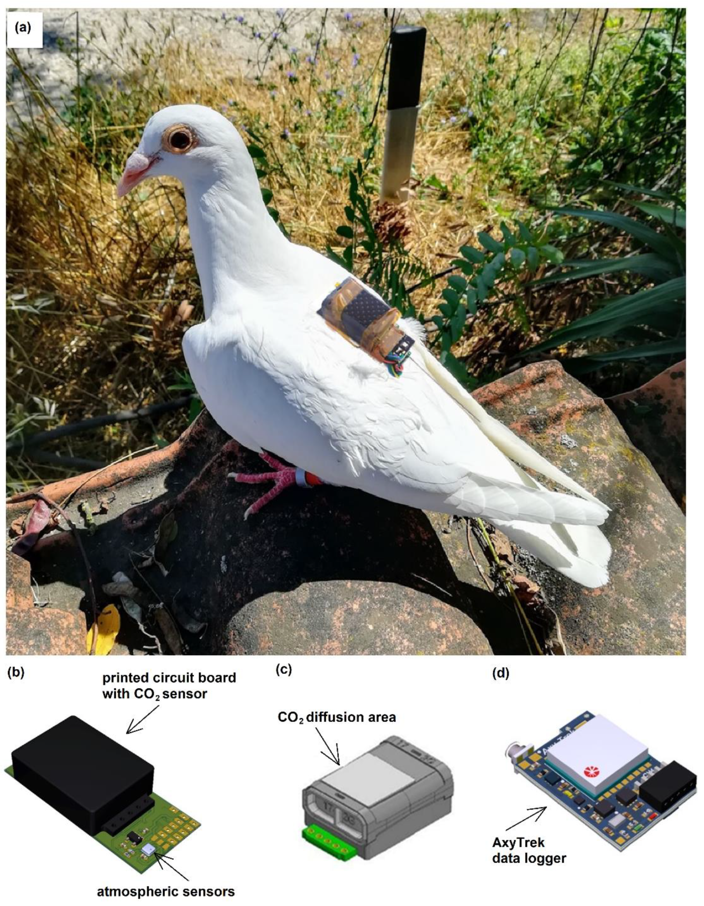
2.1. Development and Design of the Air Sampler

The development of the miniaturized air samplers used in the present study is carried out in collaboration with a private company specialized in devices for animal tracking (Technosmart Europe S.r.l., Rome, Italy). The device is based on the integration of a set of sensors on an existing GPS data logger with a wire antenna powered by a 200 mA LIPO battery (AxyTrek).
The boards and the battery are arranged in a flat and aerodynamic design (50 mm × 20 mm) to reduce possible drag to the birds in flight. The weight of the complete system (Figure 1) is 14.6 g, including the battery, and therefore at the limit of the recommended 3% of the bird’s body mass, considering that the pigeons weighed around 450 g [31]. In any case, the units are used for short-term deployments of 1–2 h.
The atmospheric sensors (BME280 Environmental sensor, Bosch Sensortec, Reutlingen, Germany) measure temperature (operational range: −40–85 °C, absolute accuracy: ±1 °C, resolution: 0.01 °C), barometric pressure (operational range: 300–1100 hPa; absolute accuracy: ±1 hPa, resolution: 0.18 hPa), and relative humidity (operational range: 0–100%, absolute accuracy: ±3%, resolution: 0.008%). The CO2 sensor (article n. 006-0-0007, Senseair Sunrise, Senseair AB, Delsbo, Sweden) is based on non-dispersive infrared (NDIR) technology and could measure CO2 concentrations from 400 to 5000 ppm, with an accuracy of ±30 ppm + 3% of reading (operating range temperature: 0–50 °C, operating range relative humidity: 0–85%). The CO2 sensor measures the light absorption emitted by a light-emitting diode (LED) into a dark chamber employing a photodiode (Figure 1). The number of CO2 particles contained in the airflow is related to the light intensity detected by the photodiode at a specific wavelength, which for CO2 is 4.26 µm. The CO2 sensor measures 33.5(L) × 19.7(W) × 11.5(H) mm3 and weighs 5 g.

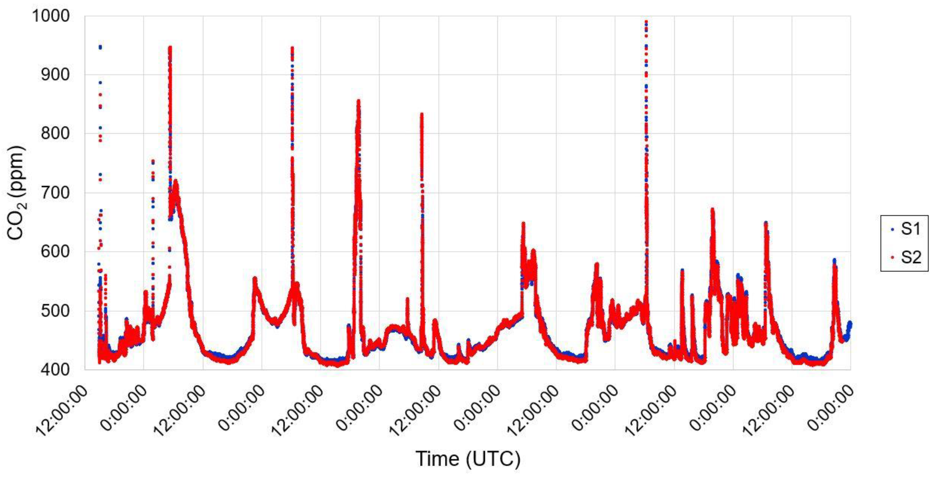
2.2. CO2 Calibration and Configuration of Environmental Sensors

A variety of calibration options are made available for the CO2 sensors by the producer, such as the Automatic Baseline Correction (ABC) algorithm [32] and manual calibration. The former works in the background over 180 h cycles, provided the sensor is exposed to “fresh air” (a customizable baseline concentration value, 400 ppm by default) at least once during the cycle. For each cycle, the sensor stores the lowest value recorded, which is assumed as the “fresh air” reference to calculate a correction factor for the data, ensuring data is reliable in the long run. The latter requires the use of a reference gas mixture and does not correct drift in long-term acquisitions.
For this study, being the data collected only for short periods during homing flights, we ensured different tags have similar sensitivity. Therefore, CO2 sensors were placed indoors for a week-long test, close to an open window, in a room occasionally occupied, increasing CO2 levels significantly. As shown in Figure 2, the two sensors tested show very similar sensitivity, with comparable responses to variations in CO2 concentration in the test room. Granger tests were performed over all the combinations of sensors, testing whether one-time series predicted the other and vice versa. All tests were highly significant (p < 0.001), meaning that every timeseries is predictable by the other.
CO2 concentrations were acquired with a sampling frequency of 0.42 Hz. This is the default value for the Senseair Sunrise, which collects eight samples per measurement. A sample takes less than 300 ms, producing a period of 2.4 s for each complete measurement. The response time is reported to be less than 30 s. This is the time needed for the sensor to read 90% (namely, T90%) of the true gas concentration, in an enclosure that changes from 8500 ppm to 400 ppm and the opposite with a gas flow rate of 1 L/min. Details about the ABC algorithm, pressure dependence, and measurement period can be found in the sensor user manual [33].
Atmospheric pressure has been found to produce a 1.6% change in CO2 readings for each 10 hPa deviation from a mean sea-level pressure (MSLP) of 1013.25 hPa. During the field campaign, the atmospheric pressure varied between 986.0 hPa and 1021.0 hPa, producing a maximum deviation of 26.9 hPa from the MSLP. This corresponds to a maximum error of 4.3% in the CO2 readings. Only 2.3% of data used in the present study have pressure with a deviation >10 hPa from the MSLP and CO2 values exceeding 625 ppm, being therefore concerned by an error greater than 10 ppm.
Temperature, air pressure, and relative humidity were collected at 1 Hz. The response time for the humidity sensor is 1 s, calculated as the time needed for the sensor to reach 63% of the final value (namely, T63%) when going from 90% to 0% or vice versa [34]. During the field campaign, the maximum daily variation in relative humidity was 49%.

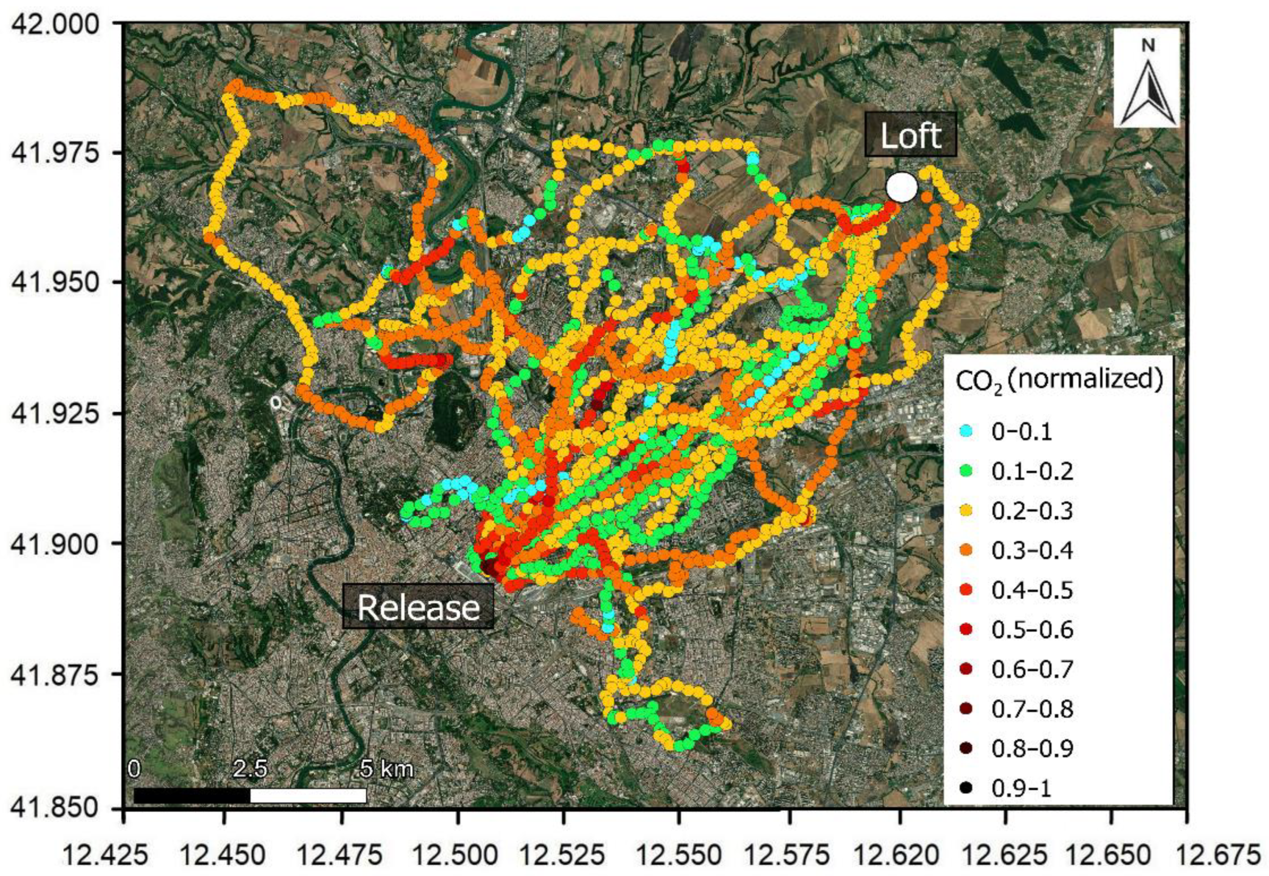
2.3. Study Area and Sample Collection

The experimental campaign, carried out from January to June 2021, involved the repeated release of homing pigeons equipped with the air sampler data logger near the campus of the University of Rome “La Sapienza” (41.90°N, 12.51°E) in downtown Rome (Italy), i.e., in a highly urbanized and moderately polluted area. The loft (41.58°N, 12.37°E) was located about 13 km northeast of the release site, about 3 km out of the “Grande Raccordo Anulare”, the highly trafficked ring road that encircles Rome.
During their flight back to the loft, homing pigeons passed through areas with different degrees of urbanization, land use, and pollution levels, i.e., they were expected to fly across a gradient of decreasing CO2 concentration to reach their loft in the countryside. Moreover, sampling was expected to take place in the range of altitudes between 0 and 150 m above ground level (m a.g.l.), the typical flight range of pigeons. All the releases were carried out on working days and most of the releases took place early in the morning (at about 07:00 UTC) to capture the increase in CO2 concentration associated with morning traffic rush hours. A few pigeons were released at later hours (from 09:00 UTC up to 13:00 UTC). A list of the release trials, together with details about distance flown, duration of flights, and statistics on measured CO2 is shown in Table A1.
For the trials, twelve adult homing pigeons were equipped with the devices following the procedure described for GPS loggers by [35]. Briefly, the birds were habituated to carry the load using a plastic dummy (of the same weight and size as the logger) attached with a Velcro strip on their back, on a dorsal area between the wings. The hard side of the Velcro strip (30.0 × 20.0 mm) was attached using a neoprenic glue on an area of half-cut feathers—therefore without causing pain and discomfort to the birds—whereas the soft side of Velcro was attached at the base of both the dummy and the device. Pigeons carried the dummy for two weeks before the experimental release. In general, they already resumed their normal behaviour (feeding, daily flight, reproductive activities) on the day after the attachment of the dummy. On the day of the release, birds were taken from the loft and gently placed in a wooden box for transportation to the city centre by car (about a 30 min trip). Ten minutes before the release, the dummies were replaced with the air samplers, and then, pigeons were released in flocks of 3–4 birds with 1–2 birds equipped with the air sampler and the remaining wearing the dummies. Releases were carried out only with good meteorological conditions, avoiding rainy and windy days. On their arrival at the loft, birds were handled to recover the loggers and reposition the dummy. The data were downloaded using dedicated software to obtain a CSV file containing timeseries of GPS position, temperature, air pressure, humidity, and CO2 concentration.

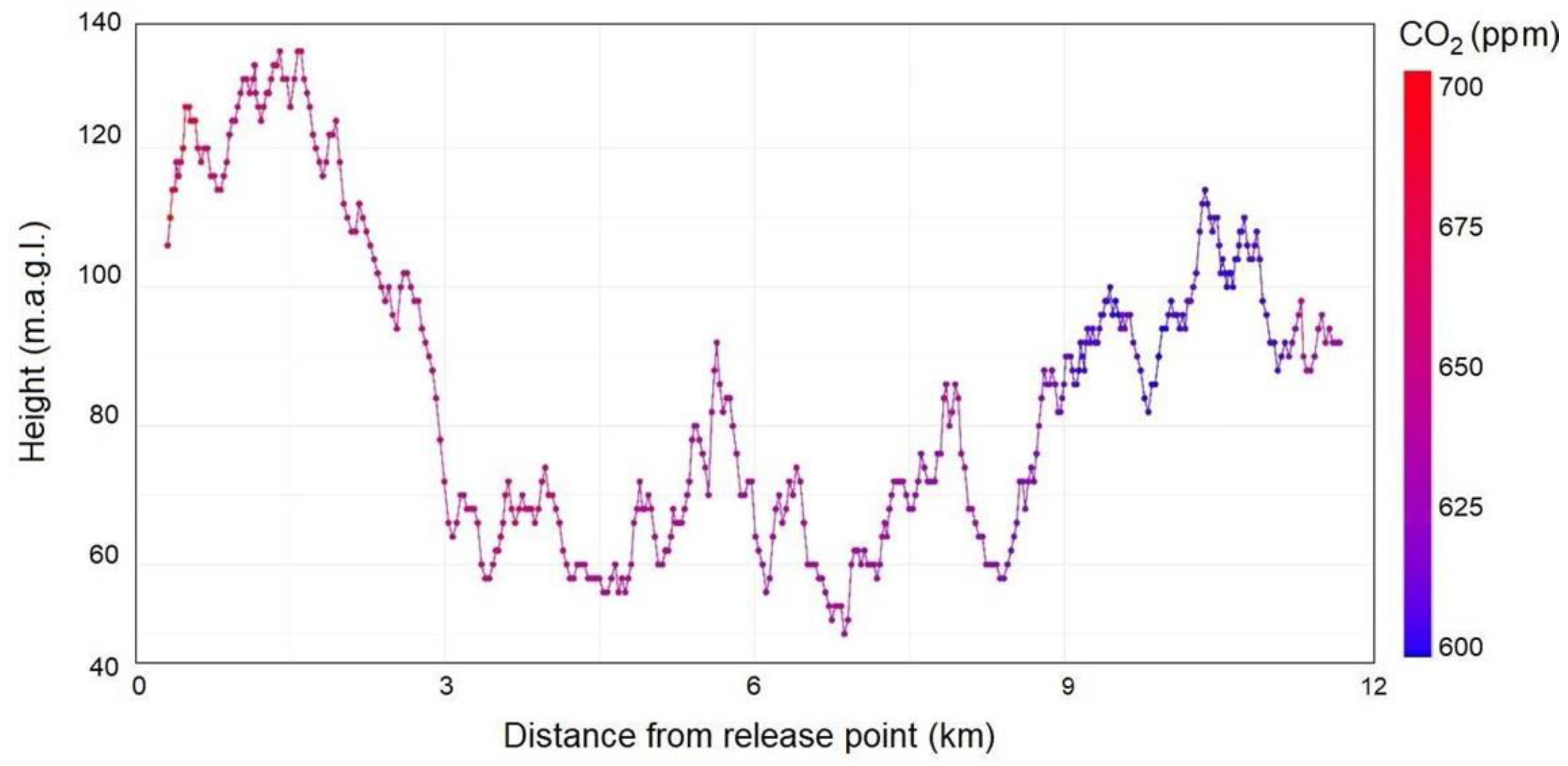
2.4. Data Processing

Firstly, data collected by the various sensors were visually inspected to ascertain whether the tracks were complete. The GPS locations were plotted on the city map using QGIS software (version 3.10), official project of the Open Source Geospatial Foundation (OSGeo, Beaverton, OR, USA), and the symbols corresponding to the GPS positions were colour-coded along a gradient according to the CO2 level for each of the sensors used allowing for a first data inspection.
GPS data were pre-processed following the procedure proposed by [36]. In particular, GPS values related to velocities greater than 90 km/h and negative altitudes were discarded. Moreover, only active flight points (flight speed as measured by GPS ≥ 0.1 m/s) were considered for the analysis and pigeon tracks were cut on their arrival by excluding points in a circular area of 500 m centred on the loft. Pigeon tracks were merged with level 3 Corine Land Cover (CLC) data [37] and classified as “urban fabric” (CLC classes from 1.1.1 to 1.3.3), “green urban areas” (CLC classes 1.4.1 and 1.4.2), and “agricultural areas” (CLC classes from 2.1.1 to 2.4.4). Points along the Tiber River (CLC class 5.1.1) were assimilated into green urban areas. No other land cover classes were crossed during the flights. It is worth noticing that CLC classification probably does not offer the optimal resolution for land cover features. Nonetheless, to the best of our knowledge, this is the most recent and accurate dataset available for the area under investigation. To improve the representation of the examined area, a shapefile of roads [38] was used to classify points lying within 50 m of streets, considering both motorways and small urban roads.
Then, CO2 values were regressed against land cover, intersection with streets, and time of release (i.e., the hour of day and month of the year). Whether to include in the analysis temperature, humidity, barometric pressure, flight speed, flight altitude, distance from the release point, and interaction between the latter two variables was decided via Akaike Information Criterion (AIC) [39] using stepwise elimination (function “buildmer” from package “buildmer” [40]). Multicollinearity was checked by calculating the variance inflation factor (VIF, function “vif” from package “car” [41]). Distance from the release point was included due to an increasing presence of agricultural areas moving out of the city centre towards the loft. From preliminary inspection (see colours in Figure 3), the distance from the release point seemed to be related to CO2 values and, therefore, it was considered as a continuous variable, providing information on land cover. A linear mixed effect model (function “lme” from package “nlme” [42]) with pigeon ID as a random effect was run, testing the random effects by comparing the model to a generalized least squares regression only containing the fixed predictors.
Data were highly autocorrelated, and while this did not affect regression coefficient estimates, it might have produced biased standard errors, making the coefficient significance unreliable [43]. To account for this, data were first subsampled with 15 s temporal resolution (corresponding to approximately 200 m spatial resolution if birds were flying with an average velocity of about 13 m/s resulting from our GPS data). Then, the model was fitted with a continuous autoregressive structure of the first order (function “corCAR1” from package “nlme” [42]). All analyses were performed using R Statistical Software (version 4.0.3, [44]), developed by the R Foundation for Statistical Computing (Vienna, Austria).
Throughout the whole campaign, the atmospheric sensors collected about 1.9 × 10⁴ data points of active flight outside the 500 m loft buffer during 25 flights. Further subsampling to one fix per 15 s resulted in about 3.3 × 10³ points with CO2 measurements, which constitute the filtered dataset used for the following analysis.

3. Results

Figure 3 shows the paths followed by the homing pigeons during the measurement campaign and the normalized CO2 concentrations. In accordance with the details in Table A1, CO2 levels range between 410 ppm and 993 ppm. The variation in concentrations between different flights are mainly due to different land use and flight time. In fact, the CO2 peaks correspond to the measurements carried out close to major roads and during rush hour traffic. Clearly, during each flight, each pigeon can choose a different path to follow based on its experience and environmental conditions.
In Figure 4, an example of the CO2 concentration time series collected during a pigeon flight expressed as a function of the distance from the release point and of the height is given. The concentration decreases with increasing flight altitude, as expected, moving away from surface emissions, but it is strongly influenced by land use, e.g., the decrease observable at about 10 km from the release point between 80 and 100 m.a.g.l. is due to the overflight of the agricultural landscape after the “Grande Raccordo Anulare” road, characterized by few roads and buildings.
The stepwise regression reveals the full model, i.e., the one comprising all terms (see Table 1), to have the lowest AIC score. VIF is below 2.7 for all the predictors, meaning only a low correlation is found among them. Including random effects, the regression lowered the model’s AIC by 116 points (Anova test, p < 0.001), and the corCAR1 error structure lowered it by 3914 points (Anova test, p < 0.001). The full model’s conditional coefficient of determination (hereinafter, R2) was 0.69, while the marginal R2 is 0.39 [45]. Our data shows that CO2 concentrations are positively related to relative humidity (estimated: 40.71, standard error: 4.07, p < 0.001) and air temperature (estimated: 12.30, standard error: 5.61, p = 0.03) and negatively related to barometric pressure (estimates: −8.98, standard error: 5.61, p = 0.001). Regarding the temporal trend, a negative relation with both months of the year (estimated: −14.34, standard error: 4.24, p < 0.001) and time of the day (estimated: −4.32, standard error: 1.27, p < 0.001) emerged. No evidence that the sections of flight over streets measured higher CO2 levels than average was found. In some of the tracks, the overflight of the “Grande Raccordo Anulare” road determined the sudden and significant increase in the concentration of CO2 but, in general, the dense urban road infrastructure did not reveal fine-scale differences within the urban environment itself (see Figure 3). However, lower CO2 concentrations over urban green areas compared to pure urban fabric (estimated: −6.76, standard error: 3.55, p = 0.057) were found. The interaction term between distance and height showed a positive relation with CO2 (estimated: 4.70, standard error: 1.18, p < 0.001), unveiling a complex three-dimensional spatial pattern of diffusion. In fact, while for low heights lower CO2 values moving outside of the city were observed, the relationship reversed for greater heights. It is worth noting the small but positive effect of flight speed on CO2 (estimated: 1.87, standard error: 0.82, p = 0.02), which would need to be explained in a larger atmospheric dynamics context. A graphical summary of the model estimates is presented in Figure 5, while the full summary is given in Table 1.

4. Discussion

The atmospheric CO2 concentrations measured along the return journey of the pigeons released in the centre of Rome (see for example Figure 4) showed an evident negative gradient with increasing distance from the release point, as supported by the linear mixed effects regression model. The highest concentrations were recorded in downtown Rome, i.e., close to the release point, with a gradual decrease moving towards suburban and rural areas. This is consistent with the findings of other studies that have shown the presence of an “urban CO2 dome” [46] and a close relationship between CO2 levels and population density, in turn associated with the high traffic volume of urban centers [47]. The average concentration obtained considering only the samples measured over the “urban fabric” land cover class was 563 ppm, with average levels decreasing over “agricultural areas” (546 ppm) and even more so over “green urban areas” (538 ppm), highlighting the positive effect of urban greening on air quality [48]. All the average concentrations are well above the mean global atmospheric CO2 concentration provided by [49] and referred to 2020, i.e., 412.5 ppm. In the urban environment, the concentration is comparable with results from [11], who carried out measurements in a highly urbanized and moderately polluted area in Rome, close to that investigated in this work, during the traffic rush hours. As expected, the values measured here for the “urban fabric” were slightly lower than the findings by [11], who carried out measurements along the road at the pedestrian level. A similar trend was also identified by [50], who examined the spatial variability of the near-surface CO2 concentration in Shanghai (China). In the same time interval (from 9:00 to 11:00 AM) and the same season (spring), Liu et al. [50] identified a clear concentration decrease moving from the transportation area to crops, with a positive correlation with the percentage of impervious surface cover and a negative correlation with the percentage of vegetation cover. The positive relation between CO2 level, air temperature, and relative humidity agrees with [11], who measured the highest CO2 values with high temperatures and low wind speeds, and with [51], who identified a slight influence of temperature and relative humidity on the CO2 concentration. Furthermore, the positive relation between CO2 levels and near-surface air temperatures was also highlighted by [51] at the remote sites of Mauna Loa (USA) and Point Barrow (USA). The slightly negative relationship between CO2 and time of day, considering that most releases were carried out before 09:30 UTC, suggests that the convective mixing generated by the presence of solar radiation and the photosynthetic absorption of CO2 by vegetation have a significant effect on the space-time redistribution of CO2, which, therefore, accumulates more in the layers of the atmosphere closest to the ground during the night and the early morning hours [46]. Moreover, this negative relation is presumably traceable also to factors we were unable to include in our model, such as the traffic rate, which is lower later in the morning after rush hours and shows a shift forward going towards the summer months. Of course, later morning hours are also associated with warmer air temperatures, therefore missing explanatory variables would confound the relationship between CO2 and temperature, which we would expect to be significantly positive. To be able to verify this relation, it would be necessary to design measurement campaigns with continuous releases during the same day, allowing for the in-depth investigation of the PBL development and the photosynthetic absorption.
The negative relation with the month of the year is likely due to the CO2 seasonal fluxes between the atmosphere and the land biosphere, which overlap with fossil fuel emissions, giving rise to large carbon dioxide seasonal variations [52].
Finally, the model shows a poor relation between CO2 atmospheric concentration, flight speed, and altitude. This could be justifiable considering that the flight altitudes were mostly below 150 m a.g.l., i.e., widely within the PBL, where the presence of turbulent fluxes determines a high degree of pollutants mixing and a high space-time homogeneity.
The meteorological and air quality measurements, acquired with high spatial-temporal resolution in the vertical profiles of urban and non-urban environments can be integrated and compared with the data measured at the ground level, allowing for the detailed characterization of atmospheric parameters within the PBL. This involves hypotheses and assumptions that are not always truthful: during the flight, sensors are in continuous movement, while ground-based measurements are typically carried out by fixed stations, located in strategic points of the city. In the case of the homing pigeons used in our study it follows that, even if a release takes place near a ground station, the comparison could only be carried out for a few seconds after the release, i.e., when the bird is still close to the station itself. In addition, birds decide themselves both the route and the altitude during the entire journey, resulting in a non-predictable trajectory of their flight at a fine scale. Furthermore, if, as in the present study, homing pigeons are used, they require in-group releases and have to familiarize themselves with specific locations of release, so that they can learn the route back to their loft. In fact, if the same pigeon is released several times at the same point, it will tend to memorize the shortest, straightest path to the loft and will tend to follow it on each subsequent flight [53]. This means that the paths will tend to become similar with time, with the advantage of making the measurements gathered in different releases more comparable.
Another fundamental aspect of these measurements is the temporal constraint. Depending on the distance between the release point and the loft and on the individual’s experience, the pigeon can take a shorter/longer time to go back home, i.e., it will acquire a shorter/longer dataset. On one hand, this ensures that during the flight, the environmental conditions can be assumed as constant (in terms of temperature, humidity, concentrations of pollutants, etc.), but, on the other hand, short flights do not allow the study of the daily PBL evolution. However, this apparent limitation can be overcome by carrying out subsequent releases at different moments of the day. Another non-negligible constraint is linked to the fact that pigeons—similar to many diurnal birds—do not fly at night and in the case of bad weather conditions.
Moreover, the sensor design might influence the relationship between CO2 and other measured atmospheric variables. In our case, the absence of a casing and the direct exposure of the atmospheric sensors to solar radiation might produce higher temperatures than the actual environmental values. This could be an issue, especially if the pigeon stays still under the sun for long periods. This does not concern the data presented in this study since our model only includes flying periods. Given the optical nature of the CO2 sensor, we believe direct exposure to solar radiation does not affect gas readings. Indeed, there is no mention of exposure in the sensor documentation [33]. Nonetheless, further development of the tag will include a casing, which is essential for longer deployments. This will warrant an analysis of design-dependence on all sensor readings.
In conclusion, we demonstrated the feasibility of using birds as biomonitoring tools to sample the air quality in an urban environment. Previously, this had been attempted only in two short-lived projects that, without wishing to minimise their social impact, did not yield reproducible scientific outputs. The integrated approach used in this study has a limited disturbance to the birds. It also has a limited environmental impact, because does not require the release of probes, and the energy consumption is only related to recharging the sensors’ batteries and for data storage. This study was based on the use of data loggers, which must be recovered to download the data. With homing pigeons, this was easily done but can be difficult with wild birds. Moreover, this technological limit is being overcome, thanks to already available transmitters that can be integrated with the devices and are capable of sending real-time measurements through the fourth generation (4G) technologies. In this manner, it will be possible to monitor cities and other environments through wild species with a high temporal resolution, reducing costs and bureaucratic limitations and, thus, allowing for intervening even in emergency phases. Technological improvements and sensor miniaturization are increasing the scope of animal ecology, making animal tracking a useful way to gather high-resolution data about the environment in which they live [54]. This kind of development in the science of biologging has already been applied to the marine environment, but studies in terrestrial or aerial habitats are scant [17]. Birds are a valuable animal group in biomonitoring studies [55]. In particular, species able to perform controlled flights, such as homing pigeons, have been often used for studies on air pollution. Such studies have been mostly carried out in an ecotoxicological framework, usually requiring animal sacrifice and collecting data for limited periods [56,57,58,59]. To the best of our belief, this is the first study on environmental pollution with virtually no impact on birds.

5. Conclusions and Future Perspectives

This study reported the development of a miniaturized air sampler, integrating a GPS logger and atmospheric calibrated sensors. The device allowed for the acquisition of measurements of physical and chemical parameters, such as CO2 concentration, barometric pressure, air temperature, and relative humidity with high spatial/temporal resolution ensured by the GPS. The air samplers were applied to homing pigeons and the results demonstrated the potential of atmospheric and air quality monitoring using birds. The air sampler developed in this study represents a low-cost, environmentally friendly, easy-to-use tool for environmental monitoring, providing enhanced observation and interpretation opportunities, with minimal effects on the well-being of the birds.
The release of homing pigeons in the urban centre of Rome (Italy) and their flight to the loft highlighted the reduction of the CO2 concentration in the layers of the atmosphere close to the ground, passing from anthropized to rural and agricultural areas.
The results show that the CO2 concentration varies considerably according to the level of urbanization, underlining the positive impact of green urban areas on air quality. Furthermore, the application of a stepwise regression reveals a positive relationship between CO2 levels, relative humidity, and air temperature. Conversely, a negative relation between CO2 concentration and distance from the point of release, month, and hour of the day has been found.
This research can be considered as a starting point for further studies, aimed at developing miniaturized sensors for the study of other atmospheric gases, wearable by other bird species (i.e., gulls) with very limited impact on their well-being, capable of flying at higher altitudes and over greater distances than pigeons. Furthermore, as mentioned, sensor technology is constantly improving, both on the side of the electronics’ performance and on the possibility of transmitting data through 4G technology. This latter development, together with the progress of sensor miniaturization, which increases the possible application on wearable devices, could provide the potential for the integration of data gathered by real-time air samplers with those from other devices as part of the Internet Of Things (e.g., [60]).

Author Contributions

Conceptualization, A.D.B., V.J. and G.D.; methodology, A.D.B., V.J. and G.D.; software, V.J.; validation, V.J.; formal analysis, A.D.B., V.J. and G.D.; investigation, A.D.B.; resources, A.D.B.; data curation, V.J.; writing—original draft preparation, A.D.B.; visualization, A.D.B.; supervision, G.D.; project administration, A.D.B.; funding acquisition, A.D.B. All authors have read and agreed to the published version of the manuscript.

Funding

This research was supported by the University of Rome “La Sapienza” with the fund named “Progetti Medi di Ateneo 2018” to Annalisa Di Bernardino. Valeria Jennings carried out her work within her PhD at the University of Tuscia.

Institutional Review Board Statement

Not applicable.

Informed Consent Statement

Not applicable.

Data Availability Statement

The data acquired during the field campaign and used for the present study can be provided on request to the corresponding author.

Acknowledgments

The authors wish to thank Cristiana Bassani, Mauro Montagnoli, and Giulio Esposito from IIA-CNR for having dedicated time and expertise to the sensor calibration at the IIA-CNR laboratory. The authors are also indebted to Ing. Marco Andreoli and Ing. Marco Scialotti from TechnoSmArt Europe S.r.l. for their dedication to the development of the air sampler. The authors also thank Matteo Trivellini for caring for the homing pigeons and Ornis italica for allowing the use of the experimental pigeons.

Conflicts of Interest

The authors declare no conflict of interest.

Appendix A

Table A1. List of pigeon releases, including departure and loft arrival times, flight duration, and track length, with a summary of CO2 values measured.
Time (UTC)FlightCO2 Concentration (ppm)
Flight NumberPigeon IDSample PointsReleaseArrivalDuration (min)Distance (km)MeanMinMedianMax
1p70151221 January 2021 08:2221 January 2021 08:3917.016.7614533610812
2p78888226 January 2021 08:2926 January 2021 09:0737.727.1568498557725
3p78848028 January 2021 07:5528 January 2021 08:4449.114.7670544661978
4p710168629 January 2021 08:1529 January 2021 11:37202.247.9564457565938
5p78875629 January 2021 08:1529 January 2021 08:4025.224.0666578652993
6p7016045 February 2021 09:055 February 2021 09:3934.017.6639572635985
7p7886695 February 2021 09:015 February 2021 10:2483.119.9587489571923
8p7884368 February 2021 08:378 February 2021 10:37120.414.3571452547903
9p56169319 March 2021 09:0219 March 2021 09:2523.118.7497476489576
10p77810071 April 2021 07:041 April 2021 12:13309.225.1562504555913
11p479687 April 2021 07:067 April 2021 12:53347.626.1466410465558
12p77812497 April 2021 07:017 April 2021 09:37156.038.3531481527696
13p472569 April 2021 08:579 April 2021 09:068.59.4455436453481
14p5614289 April 2021 08:529 April 2021 09:0614.215.2577550577963
15p4746321 April 2021 07:1921 April 2021 07:3415.414.7606514564963
16p4739123 April 2021 08:1523 April 2021 08:2813.012.8614566617702
17pG3734 May 2021 07:264 May 2021 08:0942.711.1516472516618
18pG3796 May 2021 07:186 May 2021 07:3012.613.8566516558688
19p7873517 May 2021 07:167 May 2021 07:3822.113.5567436560703
20pG3607 May 2021 07:267 May 2021 07:3812.013.7507493502547
21p3456111 May 2021 07:1811 May 2021 08:4081.915.1586492587730
22pG41011 May 2021 07:1811 May 2021 07:3517.012.8572478567699
23p684348615 June 2021 11:1916 June 2021 16:201740.382.6586528582869
24p701128715 June 2021 06:1815 June 2021 14:49510.235.8565439569793
25p70159218 June 2021 06:3518 June 2021 07:5580.516.7634538633969

References

  1. World Urbanization Prospects: The 2018 Revision; United Nations Department of Economic and Social Affairs/Population Division: New York, NY, USA, 2019.
  2. Covenant of Mayors: Reducing Energy Dependence in European Cities; European Commission: Brussels, Belgium, 2018.
  3. European Environmental Agency. EEA Greenhouse Gases—Data Viewer. 2021. Available online: https://www.eea.europa.eu/data-and-maps/data/data-viewers/greenhouse-gases-viewer (accessed on 18 January 2022).
  4. Intergovernmental Panel on Climate Change: Climate Change 2021. The Physical Science Basis Summary for Policymakers. Contribution of Working Group I to the sixth Assessment Report of the Intergovernmental Panel on Climate Change; Cambridge University Press: Cambridge, UK, 2021; p. 41.
  5. Brooks, H.E. Severe thunderstorms and climate change. Atmos. Res. 2013, 123, 129–138. [Google Scholar] [CrossRef]
  6. Estrada, F.; Kim, D.; Perron, P. Spatial variations in the warming trend and the transition to more severe weather in mid latitudes. Sci. Rep. 2021, 11, 145. [Google Scholar] [CrossRef] [PubMed]
  7. Aubinet, M.; Grelle, A.; Ibrom, A.; Rannik, U.; Moncrieff, J.; Foken, T.; Kowalski, A.S.; Martin, P.H.; Berbigier, P.; Bernhofer, C.; et al. Estimates of the annual net carbon and water exchange of forests: The EUROFLUX methodology. Adv. Ecol. Res. 1999, 30, 113–175. [Google Scholar]
  8. Xiao, J.; Zhuang, Q.; Baldocchi, D.D.; Law, B.E.; Richardson, A.D.; Chen, J.; Oren, R.; Starr, G.; Noormets, A.; Ma, S.; et al. Estimation of net ecosystem carbon exchange for the conterminous United States by combining MODIS and AmeriFlux data. Agric. For. Meteorol. 2008, 148, 1827–1847. [Google Scholar] [CrossRef]
  9. Moriwaki, R.; Kanda, M. Seasonal and diurnal fluxes of radiation, heat, water vapor, and carbon dioxide over a suburban area. J. Appl. Meteorol. 2004, 43, 1700–1710. [Google Scholar] [CrossRef]
  10. Soegaard, H.; Møller-Jensen, L. Towards a spatial CO2 budget of a metropolitan region based on textural image classification and flux measurements. Remote Sens. Environ. 2003, 87, 283–294. [Google Scholar] [CrossRef]
  11. Pigliautile, I.; Marseglia, G.; Pisello, A.L. Investigation of CO2 variation and mapping through wearable sensing techniques for measuring pedestrians’ exposure in urban areas. Sustainability 2020, 12, 3936. [Google Scholar] [CrossRef]
  12. Idso, C.D.; Idso, S.B.; Balling, R.C., Jr. An intensive two-week study of an urban CO2 dome in Phoenix, Arizona, USA. Atmos. Environ. 2001, 35, 995–1000. [Google Scholar] [CrossRef]
  13. Coutts, A.M.; Beringer, J.; Tapper, N.J. Characteristics influencing the variability of urban CO2 fluxes in Melbourne, Australia. Atmos. Environ. 2007, 41, 51–62. [Google Scholar] [CrossRef]
  14. Fehlmann, G.; King, A.J. Bio-logging. Curr. Biol. 2016, 26, R830–R831. [Google Scholar] [CrossRef]
  15. Boyd, I.L.; Kato, A.; Ropert-Coudert, Y. Bio-logging science: Sensing beyond the boundaries. Mem. Natl. Inst. Polar Res. 2004, 58, 1–14. [Google Scholar]
  16. Rutz, C.; Hays, G.C. New frontiers in biologging science. Biol. Lett. 2009, 5, 289–292. [Google Scholar] [CrossRef] [PubMed] [Green Version]
  17. Wilmers, C.C.; Nickel, B.; Bryce, C.M.; Smith, J.A.; Wheat, R.E.; Yovovich, V. The golden age of biologging: How animal-borne sensors are advancing the frontiers of ecology. Ecology 2015, 96, 1741–1753. [Google Scholar] [CrossRef] [PubMed]
  18. Jetz, W.; Tertitski, G.; Kays, R.; Mueller, U.; Wikelski, M.; Åkesson, S.; Anisimov, Y.; Antonov, A.; Arnold, W.; Bairlein, F.; et al. Biological Earth observation with animal sensors. Trends Ecol. Evol. 2022, 37, 293–298. [Google Scholar] [CrossRef]
  19. Duriez, O.; Kato, A.; Tromp, C.; Dell’Omo, G.; Vyssotski, A.L.; Sarrazin, F.; Ropert-Coudert, Y. How cheap is soaring flight in raptors? A preliminary investigation in freely-flying vultures. PLoS ONE 2014, 9, e84887. [Google Scholar] [CrossRef]
  20. Van Tatenhove, A.; Fayet, A.; Watanuki, Y.; Yoda, K.; Shoji, A. Streaked Shearwater Calonectris leucomelas moonlight avoidance in response to low aerial predation pressure, and effects of wind speed and direction on colony attendance. Mar. Ornithol. 2018, 46, 177–185. [Google Scholar]
  21. Treep, J.; Bohrer, G.; Shamoun-Baranes, J.; Duriez, O.; de Moraes Frasson, R.P.; Bouten, W. Using high-resolution GPS tracking data of bird flight for meteorological observations. Bull. Am. Meteorol. Soc. 2016, 97, 951–961. [Google Scholar] [CrossRef]
  22. Allatt, H.T.W. The Use of Pigeons as Messengers in War and the Military Pigeon Systems of Europe. R. United Serv. Inst. J. 1886, 30, 107–148. [Google Scholar] [CrossRef]
  23. Available online: https://www.bbc.com/news/world-middle-east-40042260 (accessed on 20 September 2022).
  24. Neubronner, J. Die Photographie mit Brieftauben. In Denkschrift der Ersten Internationalen Luftschiffahrts-Ausstellung (ILA) zu Frankfurt a/M; Lepsius, B., Wachsmuth, R., Eds.; Springer: Berlin/Heidelberg, Germany, 1909; pp. 77–96. [Google Scholar]
  25. Steiner, I.; Bürgi, C.; Werffeli, S.; Dell’Omo, G.; Valenti, P.; Tröster, G.; Wolfer, D.P.; Lipp, H.-P. A GPS logger and software for analysis of homing in pigeons and small mammals. Physiol. Behav. 2000, 71, 589–596. [Google Scholar] [CrossRef]
  26. Lipp, H.-P.; Vyssotski, A.L.; Wolfer, D.P.; Renaudineau, S.; Savini, M.; Tröster, G.; Dell’Omo, G. Pigeon Homing along Highways and Exits. Curr. Biol. 2004, 14, 1239–1249. [Google Scholar] [CrossRef]
  27. Vyssotski, A.L.; Serkov, A.N.; Itskov, P.M.; Dell’Omo, G.; Latanov, A.V.; Wolfer, D.P.; Lipp, H.-P. Miniature Neurologgers for Flying Pigeons: Multichannel EEG and Action and Field Potentials in Combination With GPS Recording. J. Neurophysiol. 2006, 95, 1263–1273. [Google Scholar] [CrossRef] [PubMed]
  28. Available online: https://nideffer.net/shaniweb/pigeonblog.php (accessed on 20 September 2022).
  29. Available online: https://twitter.com/PigeonAir (accessed on 20 September 2022).
  30. Available online: https://edition.cnn.com/2016/03/16/europe/pigeon-air-patrol-pollution-london/index.html (accessed on 20 September 2022).
  31. Kenward, R.E. A Manual for Wildlife Radio Tagging; Academic Press: Cambridge, MA, USA, 2000. [Google Scholar]
  32. Senseair. The Senseair ABC-algorithm. Available online: https://senseair.com/knowledge/sensor-technology/sensor-technology/senseair-abc-algorithm/ (accessed on 1 July 2022).
  33. Senseair. Customer Integration Guidelines. Senseair Sunrise and Sunlight CO2. Document TDE7318, Rev 11. 2019. Available online: https://rmtplusstoragesenseair.blob.core.windows.net/docs/Market/publicerat/TDE7318.pdf (accessed on 1 July 2022).
  34. Bosch. BME280—Data Sheet. Document BST-BME280-DS001-23. Rev 1.23. 2022. Available online: https://www.bosch-sensortec.com/media/boschsensortec/downloads/datasheets/bst-bme280-ds002.pdf (accessed on 1 July 2022).
  35. Biro, D.; Guilford, T.; Dell’Omo, G.; Lipp, H.P. How the viewing of familiar landscapes prior to release allows pigeons to home faster: Evidence from GPS tracking. J. Exp. Biol. 2002, 205, 3833–3844. [Google Scholar] [CrossRef] [PubMed]
  36. Gupte, P.R.; Beardsworth, C.E.; Spiegel, O.; Lourie, F.; Toledo, S.; Nathan, R.; Bijleveld, A.I. A guide to pre-processing high-throughput animal tracking data. J. Anim. Ecol. 2021, 91, 287–307. [Google Scholar] [CrossRef] [PubMed]
  37. European Environment Agency: Corine Land Cover (CLC) 2018, Version 2020_20u1. Available online: https://land.copernicus.eu/pan-european/corine-land-cover/clc2018 (accessed on 18 January 2022).
  38. OpenStreetMap Contributors. Extracts Created by BBBike. Available online: https://extract.bbbike.org?sw_lng=12.322&sw_lat=41.811&ne_lng=12.832&ne_lat=42.034&format=shp.zip&city=roma&lang=en (accessed on 24 June 2021).
  39. Burnham, K.P.; Anderson, D.R. Model Selection and Multimodel Inference: A Practical Information-Theoretic Approach, 2nd ed.; Springer: Berlin/Heidelberg, Germany, 2002. [Google Scholar]
  40. Voeten, C. Buildmer: Stepwise Elimination and Term Reordering for Mixed-Effects Regression. R Package Version 2.3. 2022. Available online: https://CRAN.R-project.org/package=buildmer (accessed on 1 July 2022).
  41. Fox, J.; Weisberg, S. An {R} Companion to Applied Regression, 3rd ed.; Sage: Thousand Oaks, CA, USA, 2019; Available online: https://socialsciences.mcmaster.ca/jfox/Books/Companion/ (accessed on 1 July 2022).
  42. Pinheiro, J.; Bates, D.; DebRoy, S.; Sarkar, D.; R Core Team. Nlme: Linear and Nonlinear Mixed Effects Models. R Package Version 3.1-149. 2020. Available online: https://CRAN.R-project.org/package=nlme (accessed on 1 July 2022).
  43. Nielson, S.E.; Boyce, M.S.; Stenhouse, G.B.; Munro, R.H.M. Modeling grizzly bear habitats in the Yellowhead Ecosystem of Alberta: Taking autocorrelation seriously. Ursus 2002, 13, 45–56. [Google Scholar]
  44. R Core Team. R: A Language and Environment for Statistical Computing; R Foundation for Statistical Computing: Vienna, Austria, 2020; Available online: https://www.R-project.org/ (accessed on 1 July 2022).
  45. Nakagawa, S.; Schielzeth, H. A general and simple method for obtaining R2 from generalized linear mixed-effects models. Methods Ecol. Evol. 2013, 4, 133–142. [Google Scholar] [CrossRef]
  46. Idso, C.D.; Idso, S.B.; Balling, R.C., Jr. The urban CO2 dome of Phoenix, Arizona. Phys. Geogr. 1998, 19, 95–108. [Google Scholar] [CrossRef]
  47. Velasco, E.; Pressley, S.; Allwine, E.; Westberg, H.; Lamb, B. Measurements of CO2 fluxes from the Mexico City urban landscape. Atmos. Environ. 2005, 39, 7433–7446. [Google Scholar] [CrossRef]
  48. Nordbo, A.; Järvi, L.; Haapanala, S.; Wood, C.R.; Vesala, T. Fraction of natural area as main predictor of net CO2 emissions from cities. Geophys. Res. Lett. 2012, 39, L20802. [Google Scholar] [CrossRef]
  49. NOAA. Trends in Atmospheric Carbon Dioxide. Available online: https://gml.noaa.gov/ccgg/trends/global.html (accessed on 26 January 2022).
  50. Liu, M.; Zhu, X.; Pan, C.; Chen, L.; Zhang, H.; Jia, W.; Xiang, W. Spatial variation of near-surface CO2 concentration during spring in Shanghai. Atmos. Pollut. Res. 2016, 7, 31–39. [Google Scholar] [CrossRef]
  51. Idso, C.D.; Idso, S.B.; Balling, R.C., Jr. The relationship between near-surface air temperature over land and the annual amplitude of the atmosphere’s seasonal CO2 cycle. Environ. Exp. Bot. 1999, 41, 31–37. [Google Scholar] [CrossRef]
  52. Mousavi, S.M.; Dinan, N.M.; Ansarifard, S.; Sonnentag, O. Analyzing spatio-temporal patterns in atmospheric carbon dioxide concentration across Iran from 2003 to 2020. Atmos. Environ. X 2022, 14, 100163. [Google Scholar] [CrossRef]
  53. Dell’Ariccia, G.; Dell’Omo, G.; Wolfer, D.; Lipp, H.-P. Flock flying improves pigeons’ homing: GPS track analysis of individual flyers versus small groups. Anim. Behav. 2008, 76, 1165–1172. [Google Scholar] [CrossRef]
  54. Kays, R.; Crofoot, M.C.; Jetz, W.; Wikelski, M. Terrestrial animal tracking as an eye on life and the planet. Science 2015, 348, aaa2478. [Google Scholar] [CrossRef] [PubMed]
  55. Becker, P.H. Biomonitoring with birds. In Trace Metals and other Contaminants in the Environment; Elsevier: Amsterdam, The Netherlands, 2003; Volume 6, pp. 677–736. [Google Scholar]
  56. Cizdziel, V.J.; Dempsey, S.; Halbrook, R.S. Preliminary Evaluation of the Use of Homing Pigeons as Biomonitors of Mercury in Urban Areas of the USA and China. Bull. Environ. Contam. Toxicol. 2013, 90, 302–307. [Google Scholar] [CrossRef]
  57. Tong, Y.; Zhao, X.; Li, H.; Pei, Y.; Ma, P.; You, J. Using homing pigeons to monitor atmospheric organic pollutants in a city heavily involving in coal mining industry. Chemosphere 2022, 307, 135679. [Google Scholar] [CrossRef]
  58. Cui, J.; Halbrook, R.S.; Zang, S.; Han, S.; Li, X. Metal concentrations in homing pigeon lung tissue as a biomonitor of atmospheric pollution. Ecotoxicology 2018, 27, 169–174. [Google Scholar] [CrossRef]
  59. Liu, W.X.; Ling, X.; Halbrook, R.S.; Martineau, D.; Dou, H.; Liu, X.; Zhang, G.; Tao, S. Preliminary evaluation on the use of homing pigeons as a biomonitor in urban areas. Ecotoxicology 2010, 19, 295–305. [Google Scholar] [CrossRef]
  60. Toma, C.; Alexandru, A.; Popa, M.; Zamfiroiu, A. IoT solution for smart cities’ pollution monitoring and the security challenges. Sensors 2019, 19, 3410. [Google Scholar] [CrossRef] [Green Version]
Figure 1. Photograph of the device attached on a homing pigeon (a), schematic view of printed circuit board with CO2 and atmospheric sensors (b), CO2 sensor (Senseair Sunrise, Senseair AB, Delsbo, Sweden) with the gas diffusion area represented by the white membrane (c), and AxyTrek data logger (d).
Remotesensing 14 04876 g001
Figure 2. Temporal trend of CO2 concentration during a week-long test to compare the sensitivity of two sensors (different colours).
Remotesensing 14 04876 g002
Figure 3. Map of data subsample used for the regression model (i.e., one GPS value every 15 s). The map shows the tracks of pigeons released on different days. The colour intensity depicts the CO2 concentration measured after normalization to allow for better comparison between flights.
Remotesensing 14 04876 g003
Figure 4. Example of height profile of pigeon track (flight n. 16 in Table A1) with respect to distance from the release point. Colours refer to the CO2 concentrations measured, which are higher (redder colours) close to the release point in the city centre, and lower (bluer colours) furthest from it.
Remotesensing 14 04876 g004
Figure 5. Graphical summary of the linear mixed effects regression model estimates. Dots are the coefficient estimates for each predictor (reported on the left), with lines representing the standard errors. Red and blue show negative and positive values, respectively.
Remotesensing 14 04876 g005
Table 1. Summary of best linear mixed effects model. For each predictor, the coefficient estimate, standard error, and p-value are reported. p-values below 0.05 are reported in bold.
PredictorEstimateStandard Errorp-Value
Intercept645.3726.25<0.001
Temperature12.305.610.029
Pressure−8.982.810.002
Relative humidity40.714.07<0.001
Flight speed1.880.820.021
Height−0.321.430.822
Distance from release point−17.333.09<0.001
Hour of day−4.331.27<0.001
Month of year−14.344.24<0.001
Over streets = true−0.860.890.337
Land use = agricultural0.071.490.961
Land use = green urban−6.763.550.057
Height × distance4.701.18<0.001
Publisher’s Note: MDPI stays neutral with regard to jurisdictional claims in published maps and institutional affiliations.

