
Assessing Height Variations in Qinghai-Tibet Plateau from Time-Varying Gravity Data and Hydrological Model

Abstract
:
1. Introduction
2. Study Data
2.1. Time-Varying Gravity Data
2.2. GLDAS Noah Hydrological Model
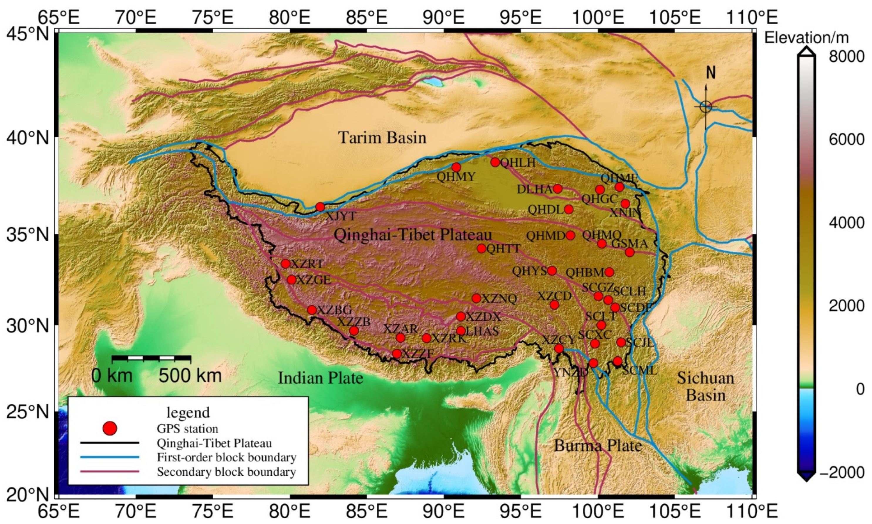
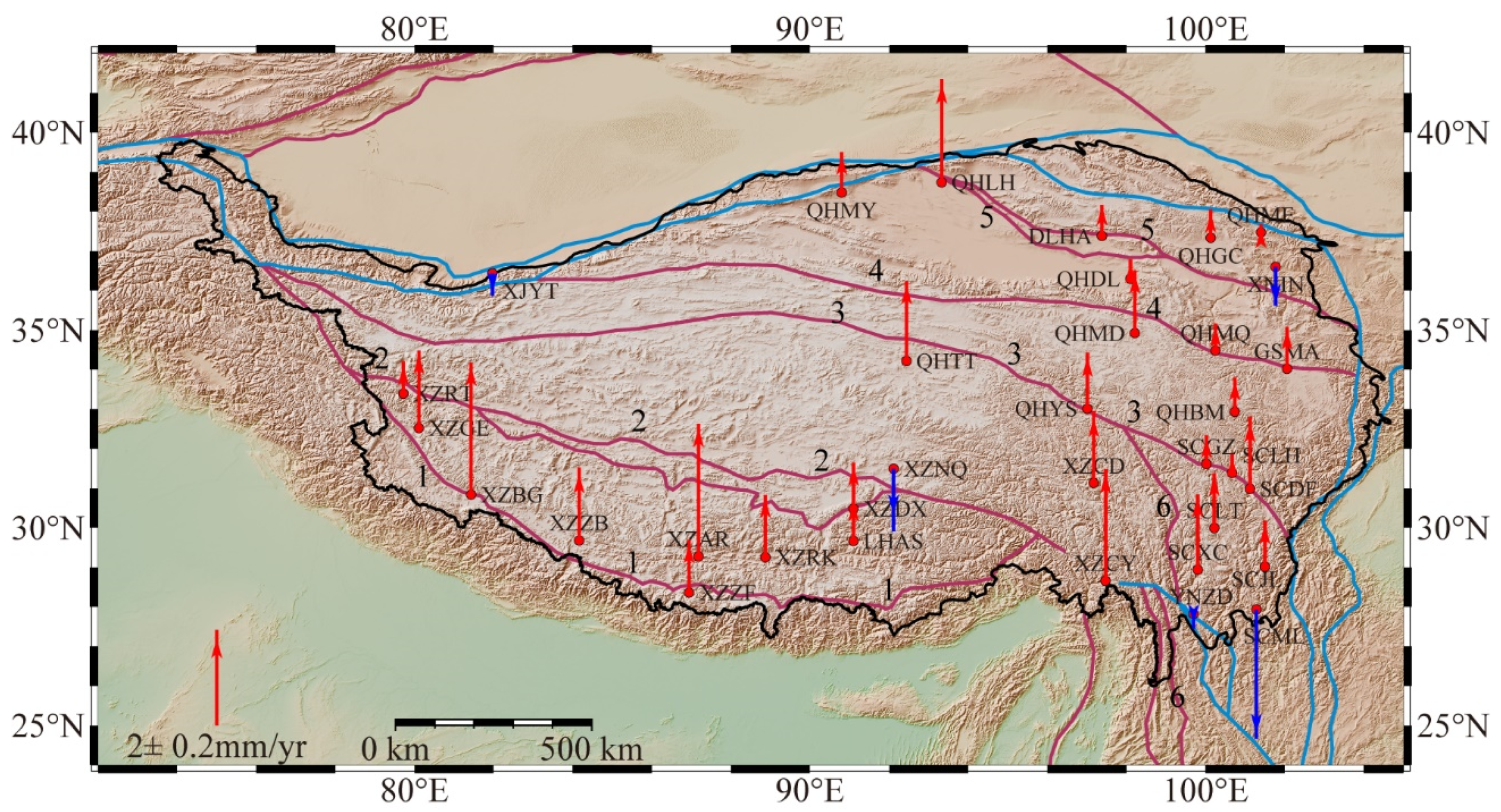
2.3. GPS Data
3. Research Methodology
3.1. Height Variations
3.1.1. Spherical Harmonic Function
3.1.2. Green’s Function
3.2. Least Square Fitting
4. Results and Analysis
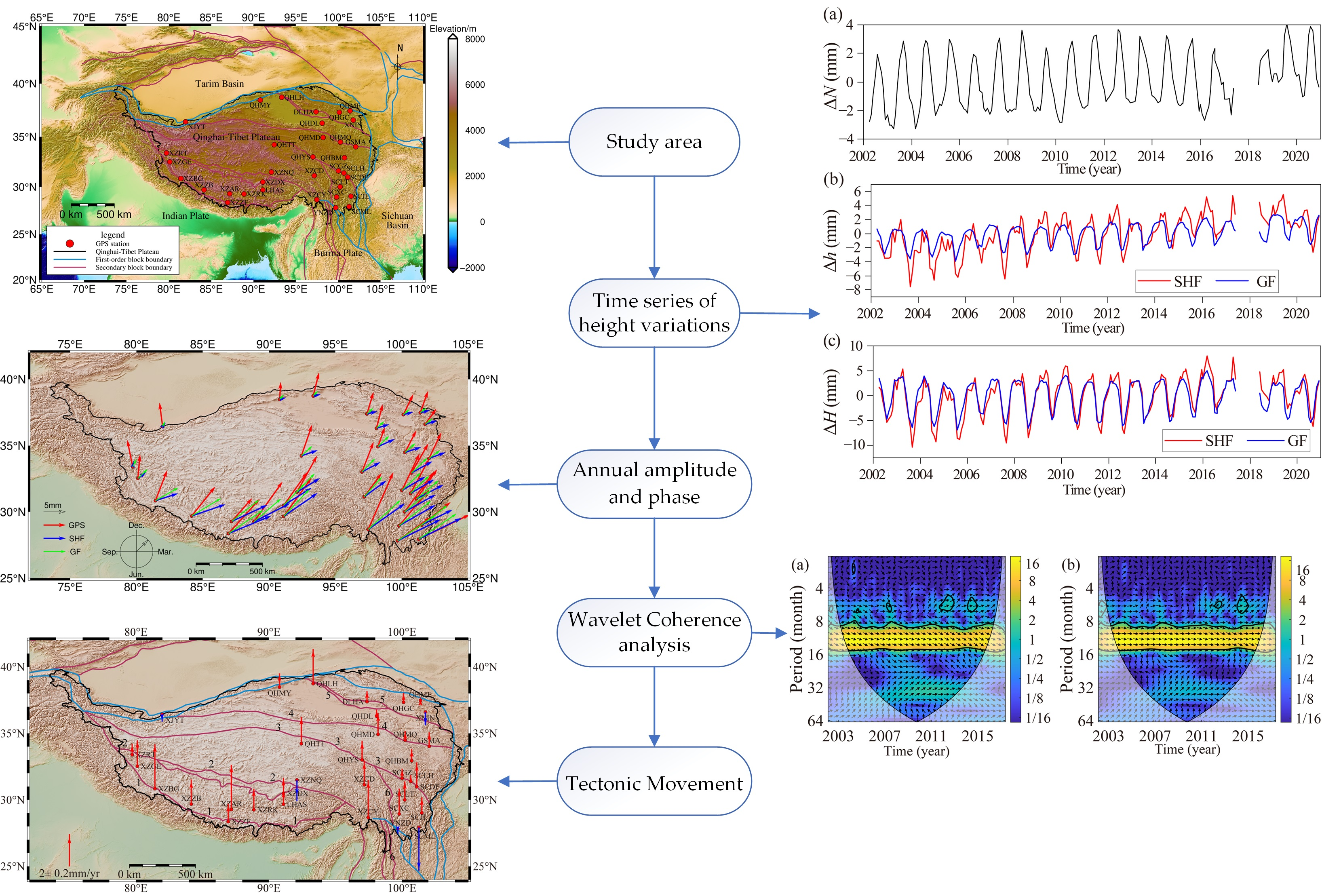
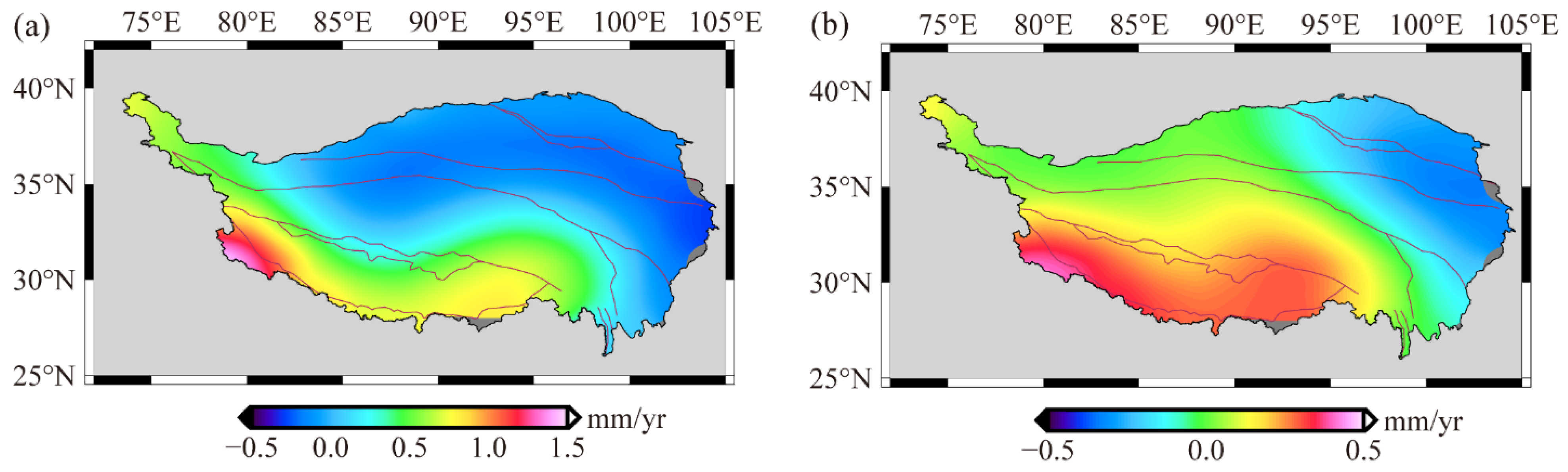
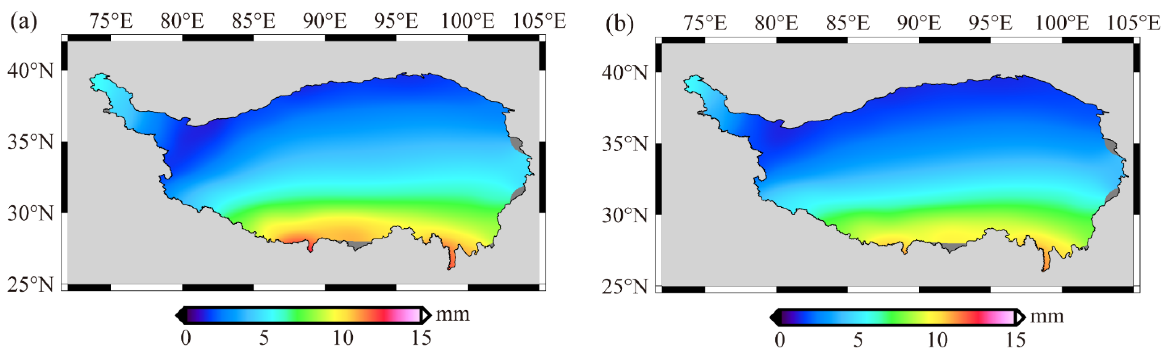
4.1. Height Variations on the QTP
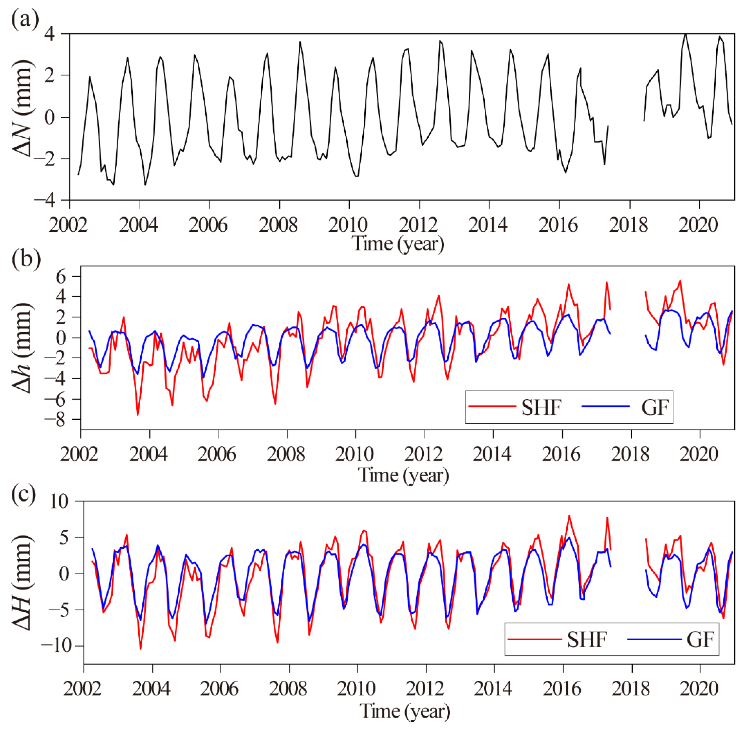
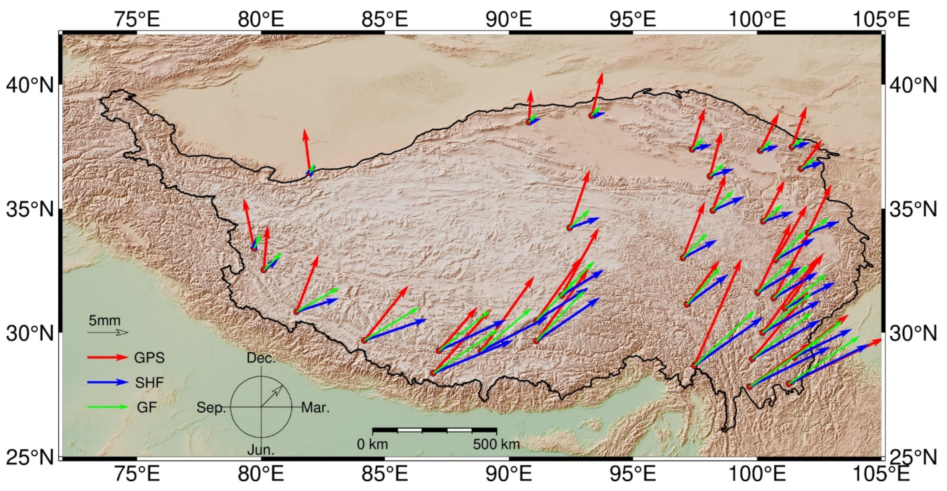
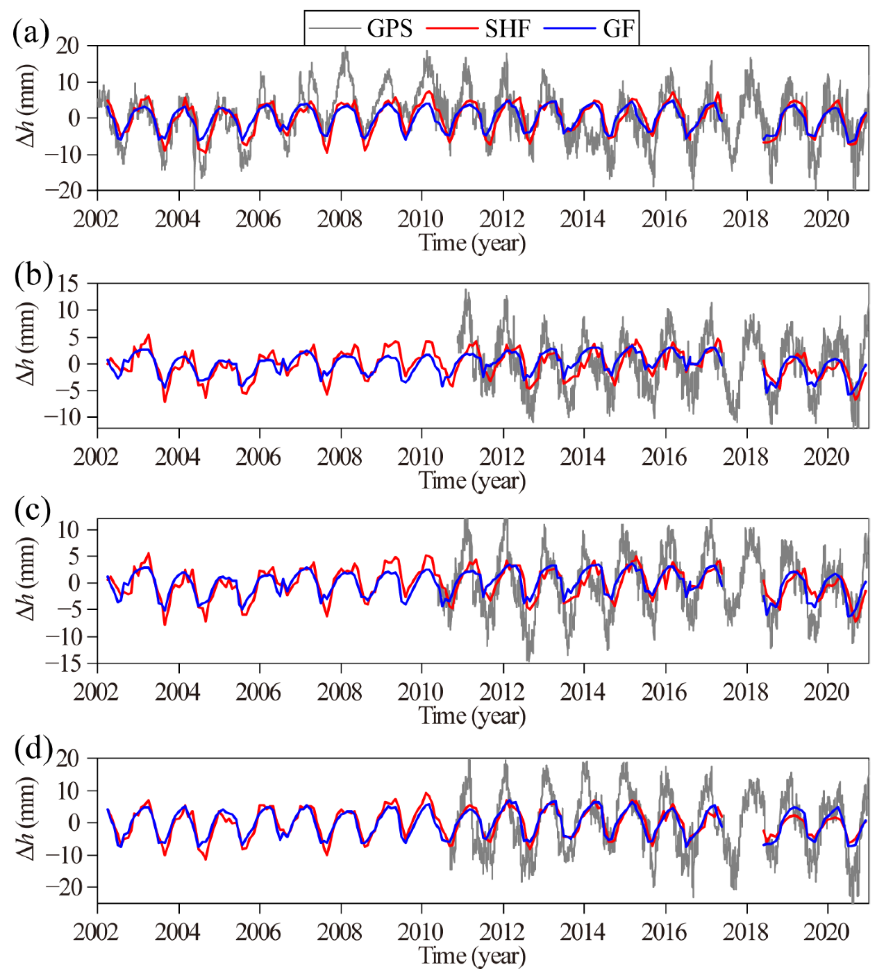
4.2. Comparison of Height Variations at GPS Stations
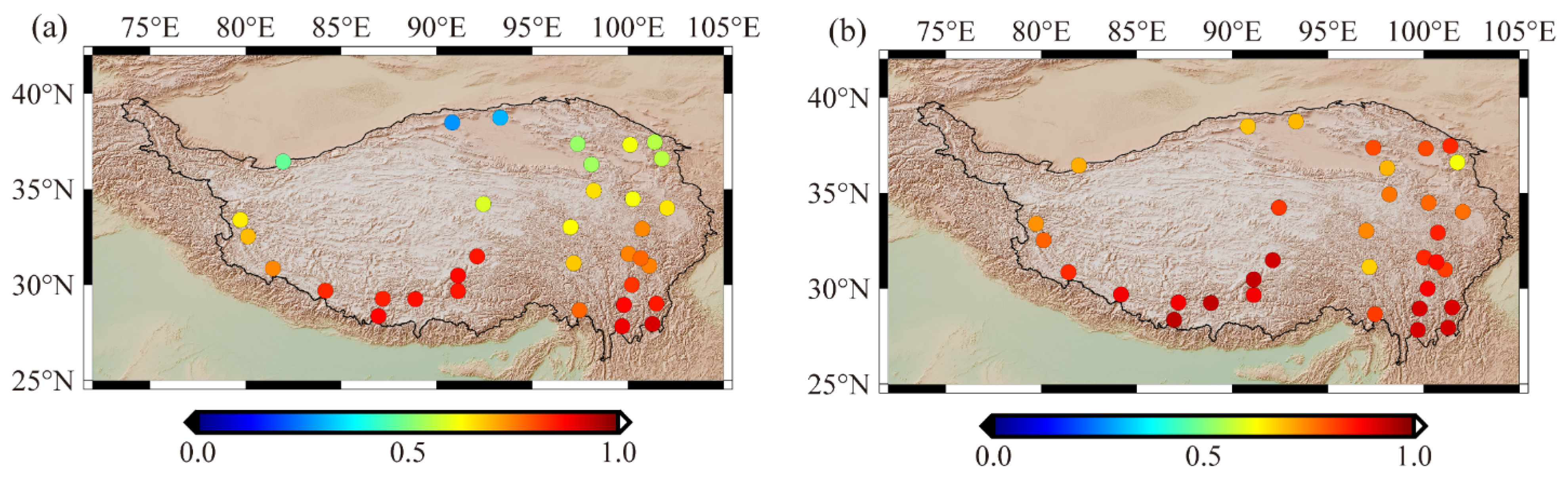
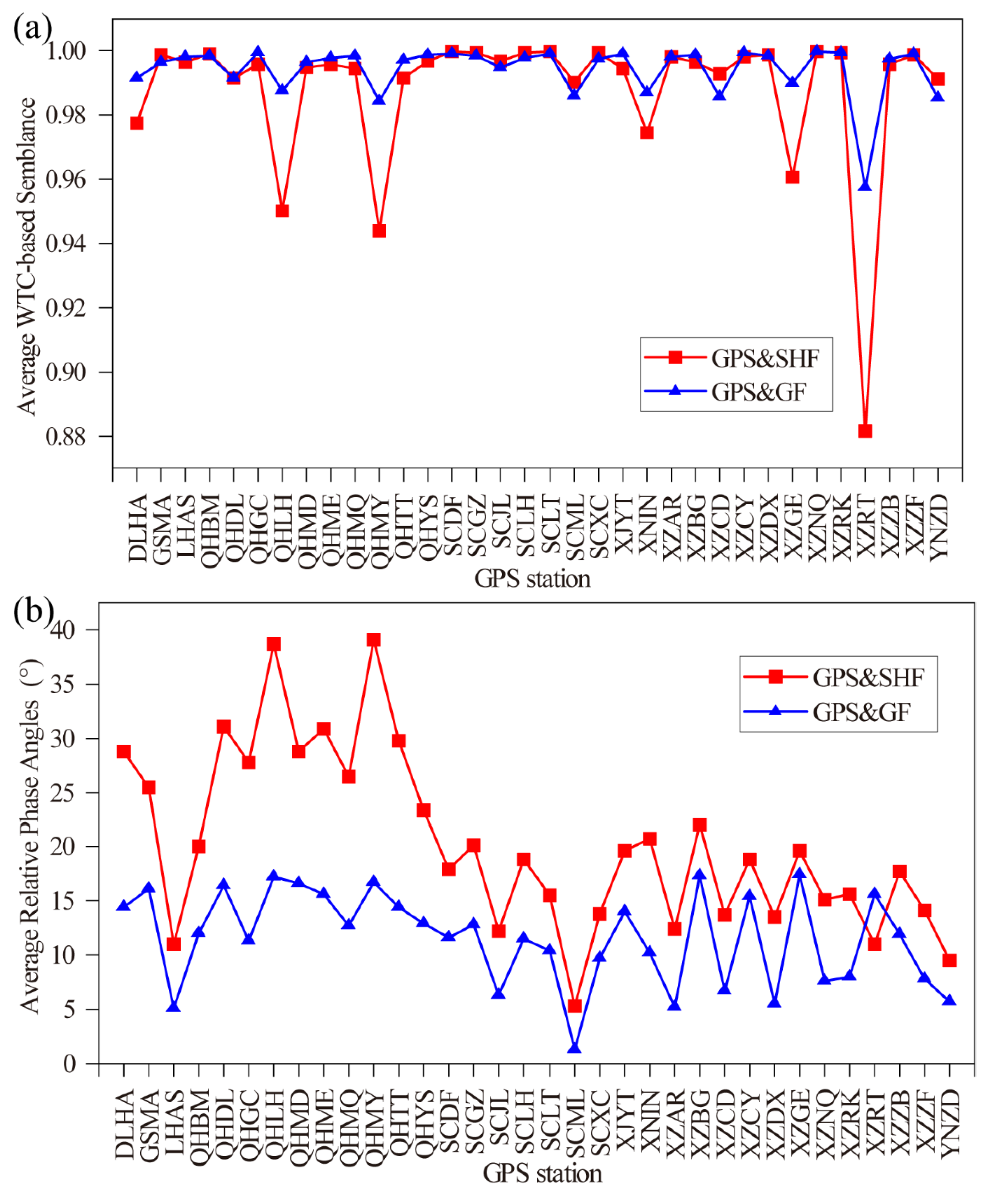
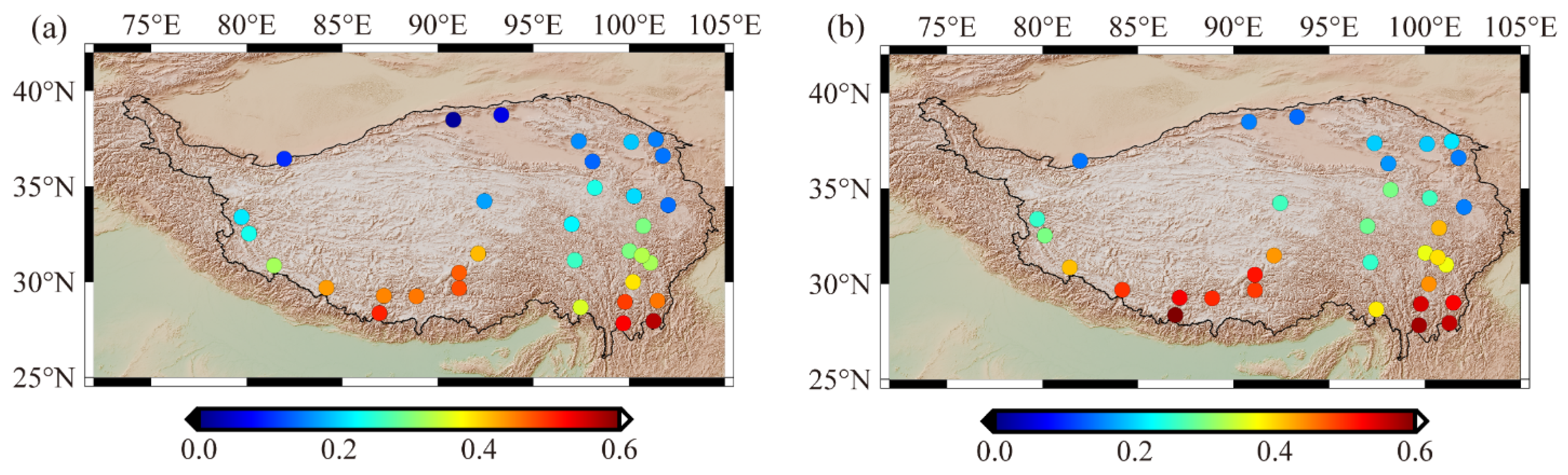
4.3. Correlation Analysis of Height Variations at GPS Stations
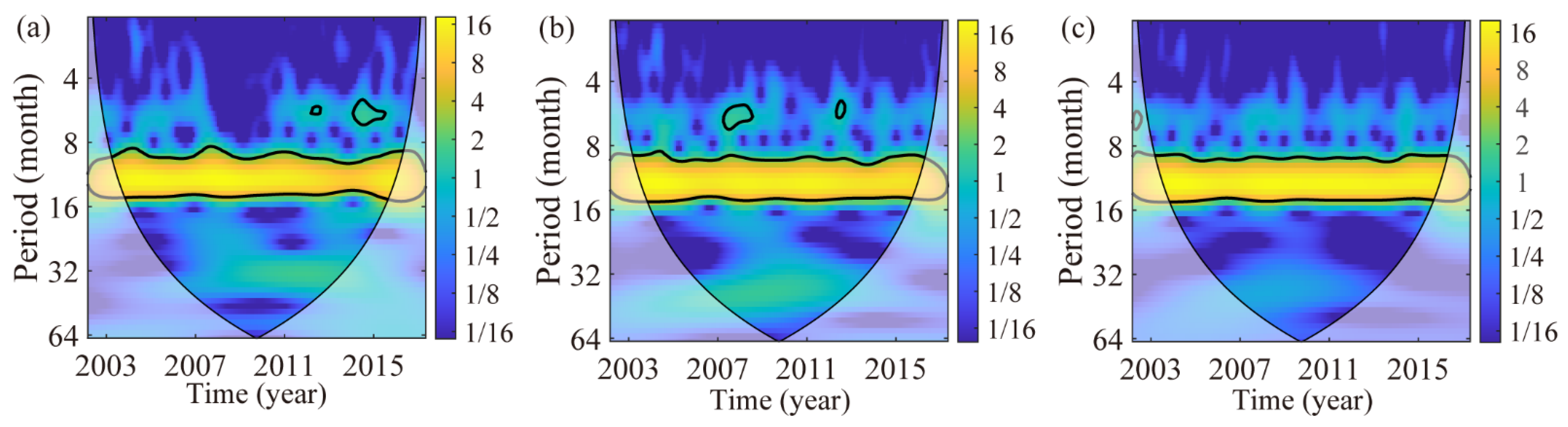
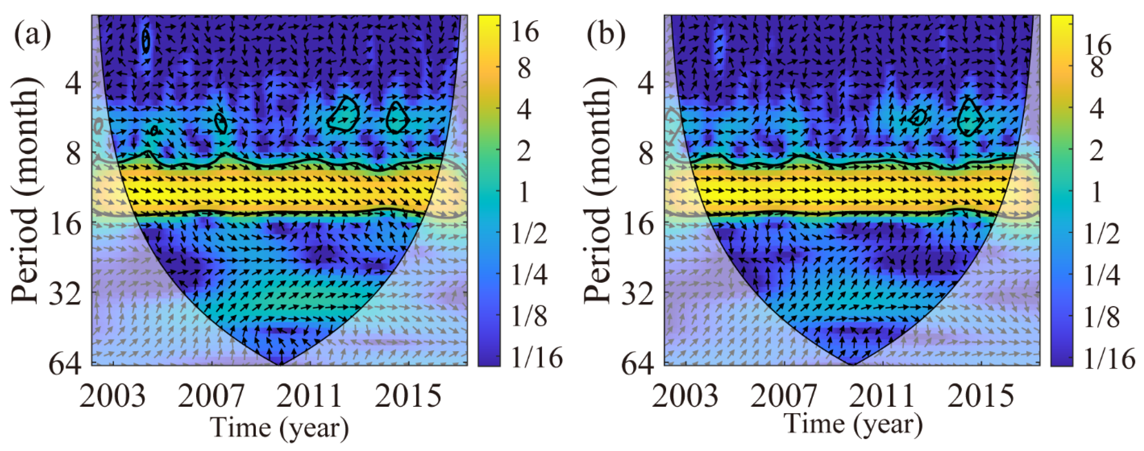
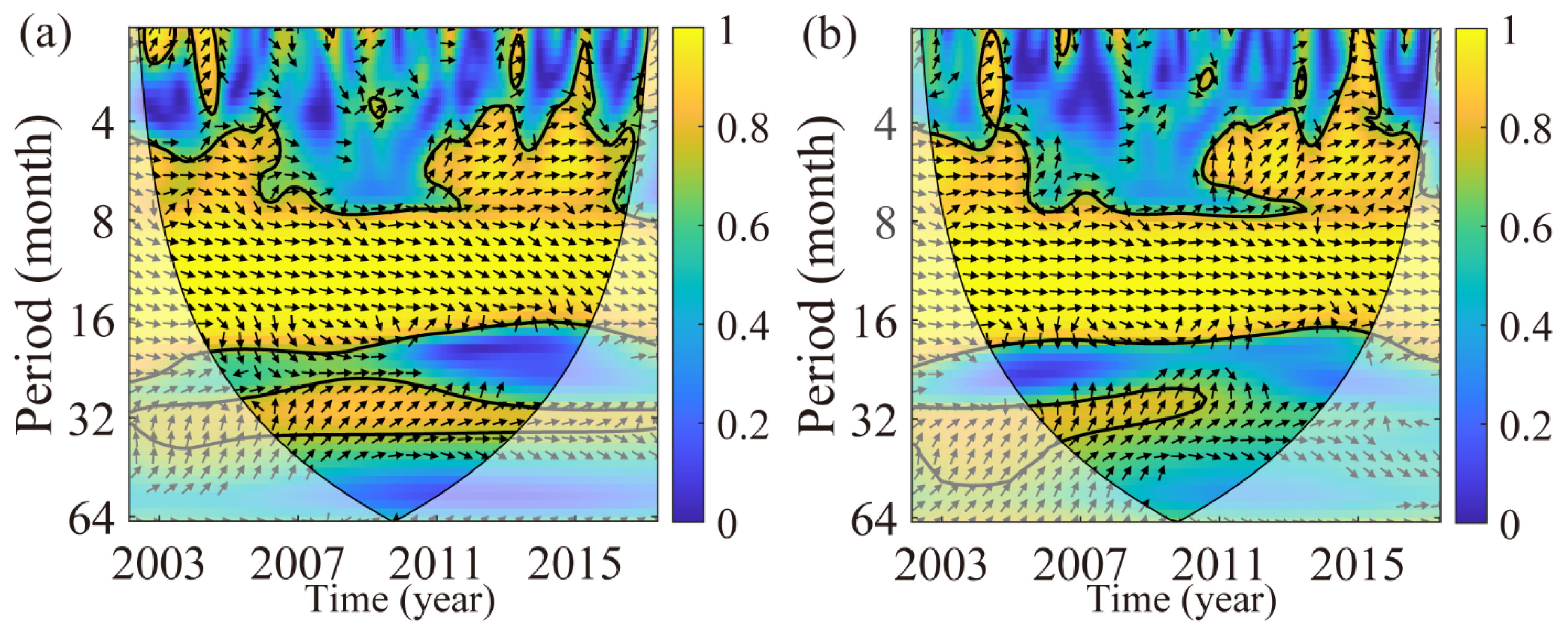
4.4. Wavelet Coherence analysis of Height Variations at GPS Stations
5. Discussions
5.1. Differences in Height Variations Derived from GRACE (-FO) and GLDAS
5.2. Quantitative Assessment of Hydrological Loading on GPS Height
5.3. Tectonic Movement Rates
6. Conclusions
Author Contributions
Funding
Data Availability Statement
Acknowledgments
Conflicts of Interest
References
- Molnar, P.; Tapponnier, P. Cenozoic tectonics of Asia: Effects of a continental collision. Science 1975, 189, 419–426. [Google Scholar] [CrossRef] [PubMed]
- Sun, W.; Wang, Q.; Li, H.; Wang, Y.; Okubo, S.; Shao, D.; Liu, D.; Fu, G. Gravity and GPS measurements reveal mass loss beneath the Tibetan Plateau: Geodetic evidence of increasing crustal thickness. Geophys. Res. Lett. 2009, 36, L02303. [Google Scholar] [CrossRef]
- Pan, Y.; Hammond, W.C.; Ding, H.; Mallick, R.; Jiang, W.; Xu, X.; Shum, C.K.; Shen, W. GPS imaging of vertical bedrock displacements: Quantification of two-dimensional vertical crustal deformation in China. J. Geophys. Res. Solid Earth 2021, 126, e2020JB020951. [Google Scholar] [CrossRef]
- Fuhrmann, T.; Westerhaus, M.; Zippelt, K.; Heck, B. Vertical displacement rates in the Upper Rhine Graben area derived from precise leveling. J. Geod. 2014, 88, 773–787. [Google Scholar] [CrossRef]
- Bawden, G.W.; Thatcher, W.; Stein, R.S.; Hudnut, K.W.; Peltzer, G. Tectonic contraction across Los Angeles after removal of groundwater pumping effects. Nature 2001, 412, 812–815. [Google Scholar] [CrossRef] [PubMed]
- Devoti, R.; Esposito, A.; Pietrantonio, G.; Pisani, A.R.; Riguzzi, F. Evidence of large scale deformation patterns from GPS data in the Italian subduction boundary. Earth Planet. Sci. Lett. 2011, 311, 230–241. [Google Scholar] [CrossRef]
- Tan, W.; Dong, D.; Chen, J.; Wu, B. Analysis of systematic differences from GPS-measured and GRACE-modeled deformation in Central Valley, California. Adv. Space Res. 2016, 57, 19–29. [Google Scholar] [CrossRef]
- Liang, S.; Gan, W.; Shen, C.; Xiao, G.; Liu, J.; Chen, W.; Ding, X.; Zhou, D. Three-dimensional velocity field of present-day crustal motion of the Tibetan Plateau derived from GPS measurements. J. Geophys. Res. Solid Earth 2013, 118, 5722–5732. [Google Scholar] [CrossRef]
- Xing, L.; Sun, W.; Li, H.; Yang, G. Present-day crust thickness increasing beneath the Qinghai-Tibetan Plateau by using geodetic data at Lhasa Station. Acta Geod. Cartogr. Sin. 2011, 40, 41–44. [Google Scholar]
- Van Camp, M.; de Viron, O.; Avouac, J.P. Separating climate-induced mass transfers and instrumental effects from tectonic signal in repeated absolute gravity measurements. Geophys. Res. Lett. 2016, 43, 4313–4320. [Google Scholar] [CrossRef]
- Chen, Z.; Chen, S.; Zhang, B.; Wang, L.; Shi, L.; Lu, H.; Liu, J.; Xu, W. Uncertainty Quantification and Field Source Inversion for the Continental-Scale Time-Varying Gravity Dataset: A Case Study in SE Tibet, China. Pure Appl. Geophys. 2022. [Google Scholar] [CrossRef]
- Tapley, B.D.; Bettadpur, S.; Watkins, M.; Reigber, C. The gravity recovery and climate experiment: Mission overview and early results. Geophys. Res. Lett. 2004, 31, L09607. [Google Scholar] [CrossRef]
- Othman, A.; Abdelrady, A.; Mohamed, A. Monitoring Mass Variations in Iraq Using Time-Variable Gravity Data. Remote Sens. 2022, 14, 3346. [Google Scholar] [CrossRef]
- Rodell, M.; Velicogna, I.; Famiglietti, J.S. Satellite-based estimates of groundwater depletion in India. Nature 2009, 460, 999–1002. [Google Scholar] [CrossRef]
- Guo, J.; Mu, D.; Liu, X.; Yan, H.; Sun, Z.; Guo, B. Water storage changes over the Tibetan Plateau revealed by GRACE mission. Acta Geophys. 2016, 64, 463–476. [Google Scholar] [CrossRef]
- Liu, X.; Zhao, N.; Guo, J.; Sun, Y.; Guo, B.; Mou, N. Equivalent water height changes over Qinghai-Tibet Plateau determined from GRACE with an independent component analysis approach. Arab. J. Geosci. 2020, 13, 179. [Google Scholar] [CrossRef]
- Goncalves, J.; Petersen, J.; Deschamps, P.; Hamelin, B.; Baba-Sy, O. Quantifying the modern recharge of the “fossil” Sahara aquifers. Geophys. Res. Lett. 2013, 40, 2673–2678. [Google Scholar] [CrossRef]
- Voss, K.A.; Famiglietti, J.S.; Lo, M.H.; de Linage, C.; Rodell, M.; Swenson, S.C. Groundwater depletion in the Middle East from GRACE with implications for transboundary water management in the Tigris-Euphrates-Western Iran region. Water Resour. Res. 2013, 49, 904–914. [Google Scholar] [CrossRef]
- Abhishek; Kinouchi, T.; Sayama, T. A comprehensive assessment of water storage dynamics and hydroclimatic extremes in the Chao Phraya River Basin during 2002–2020. J. Hydrol. 2021, 603, 126868. [Google Scholar] [CrossRef]
- Mohamed, A.; Abdelrahman, K.; Abdelrady, A. Application of Time-Variable Gravity to Groundwater Storage Fluctuations in Saudi Arabia. Front. Earth Sci. 2022, 10, 873352. [Google Scholar] [CrossRef]
- Shi, T.; Liu, X.; Mu, D.; Li, C.; Guo, J.; Xing, Y. Reconstructing gap data between GRACE and GRACE-FO based on multi-layer perceptron and analyzing terrestrial water storage changes in the Yellow River basin. Chin. J. Geophys. 2022, 65, 2448–2463. [Google Scholar]
- Geruo, A.; Wahr, J.; Zhong, S. Computations of the viscoelastic response of a 3-D compressible Earth to surface loading: An application to Glacial Isostatic Adjustment in Antarctica and Canada. Geophys. J. Int. 2013, 192, 557–572. [Google Scholar]
- Feng, W.; Shum, C.K.; Zhong, M.; Pan, Y. Groundwater Storage Changes in China from Satellite Gravity: An Overview. Remote Sens. 2018, 10, 674. [Google Scholar] [CrossRef] [Green Version]
- Farrell, W.E. Deformation of the Earth by surface loads. Rev. Geophys. 1972, 10, 761–797. [Google Scholar] [CrossRef]
- Duan, H.; Kang, M.; Wu, S.; Chen, L.; Jiao, J. Uplift rate of the Tibetan Plateau constrained by GRACE time-variable gravity field. Chin. J. Geophys. 2020, 63, 4345–4360. [Google Scholar]
- Pan, Y.; Shen, W.; Hwang, C.; Liao, C.; Zhang, T.; Zhang, G. Seasonal mass changes and crustal vertical deformations constrained by GPS and GRACE in Northeastern Tibet. Sensors 2016, 16, 1211. [Google Scholar] [CrossRef]
- Van Dam, T.; Wahr, J.M. Displacements of the earth’s surface due to atmospheric loading: Effects on gravity and baseline measurements. J. Geophys. Res. 1987, 92, 1281–1286. [Google Scholar] [CrossRef]
- Zou, R.; Wang, Q.; Freymueller, J.T.; Poutanen, M.; Cao, X.; Zhang, C.; Yang, S.; He, P. Seasonal hydrological loading in southern Tibet detected by joint analysis of GPS and GRACE. Sensors 2015, 15, 30525–30538. [Google Scholar] [CrossRef]
- Liu, J.; Fang, J.; Li, H.; Cui, R.; Chen, M. Secular variation of gravity anomalies within the Tibetan Plateau derived from GRACE data. Chin. J. Geophys. 2015, 58, 3496–3506. [Google Scholar]
- Zhang, T.; Shen, Z.; He, L.; Shen, W.; Li, W. Strain Field Features and Three-Dimensional Crustal Deformations Constrained by Dense GRACE and GPS Measurements in NE Tibet. Remote Sens. 2022, 14, 2638. [Google Scholar] [CrossRef]
- Jiao, J.; Zhang, Y.; Yin, P.; Zhang, K.; Wang, Y.; Bilker-Koivula, M. Changing Moho Beneath the Tibetan plateau revealed by GRACE observations. J. Geophys. Res. Solid Earth 2019, 124, 5907–5923. [Google Scholar] [CrossRef]
- CSR Release-06 GRACE Level-2 Data Products. Available online: https://www2.csr.utexas.edu/grace/RL06.html (accessed on 19 April 2022).
- Abhishek; Kinouchi, T.; Abolafia-Rosenzweig, R.; Ito, M. Water Budget Closure in the Upper Chao Phraya River Basin, Thailand Using Multisource Data. Remote Sens. 2022, 14, 173. [Google Scholar] [CrossRef]
- Sun, Y.; Riva, R.; Ditmar, P. Optimizing estimates of annual variations and trends in geocenter motion and J2 from a combination of GRACE data and geophysical models. J. Geophys. Res. Solid Earth 2016, 121, 8352–8370. [Google Scholar] [CrossRef]
- Loomis, B.D.; Rachlin, K.E.; Wiese, D.N.; Landerer, F.W.; Luthcke, S.B. Replacing GRACE/GRACE-FO C30 with Satellite Laser Ranging: Impacts on Antarctic ice sheet mass change. Geophys. Res. Lett. 2020, 47, e2019GL085488. [Google Scholar] [CrossRef]
- Peltier, W.R.; Argus, D.F.; Drummond, R. Comment on “An assessment of the ICE-6G_C (VM5a) glacial isostatic adjustment model” by Purcell et al. J. Geophys. Res. Solid Earth 2018, 123, 2019–2028. [Google Scholar] [CrossRef]
- Horvath, A.; Murböck, M.; Roland, P.; Horwath, M. Decorrelation of GRACE time variable gravity field solutions using full covariance information. Geosciences 2018, 8, 323. [Google Scholar] [CrossRef]
- Rodell, M.; Houser, P.R.; Jambor, U.; Gottschalck, J.; Mitchell, K.; Meng, C.J.; Aresnault, K.; Cosgrove, B.; Radakovich, J.; Bosilovich, M.; et al. The global land data assimilation system. Bull. Am. Meteorol. Soc. 2004, 85, 381–394. [Google Scholar] [CrossRef]
- King, R.; Bock, Y. Documentation for the GAMIT GPS Analysis Software; Massachusetts Institute of Technology: Cambridge, MA, USA, 2000; Available online: https://www-gpsg.mit.edu/~simon/gtgk/GAMIT.pdf (accessed on 24 April 2022).
- Liu, N.; Dai, W.; Santerre, R.; Kuang, C. A MATIAB-based Kriged Kalman Filter software for interpolating missing data in GNSS coordinate time series. GPS Solut. 2018, 22, 25. [Google Scholar] [CrossRef]
- Gelaro, R.; McCarty, W.; Suarez, M.J.; Todling, R.; Molod, A.; Takacs, L.; Randles, C.A.; Darmenov, A.; Bosilovich, M.G.; Reichle, R.; et al. The Modern-Era Retrospective Analysis for Research and Applications, Version 2 (MERRA-2). J. Clim. 2017, 30, 5419–5454. [Google Scholar] [CrossRef]
- Jungclaus, J.H.; Fischer, N.; Haak, H.; Lohmann, K.; Marotzke, J.; Matei, D.; Mikolajewicz, U.; Notz, D.; von Storch, J.S. Characteristics of the ocean simulations in the Max Planck Institute Ocean Model (MPIOM) the ocean component of the MPI-Earth system model. J. Adv. Model. Earth Syst. 2013, 5, 422–446. [Google Scholar] [CrossRef]
- Petrov, L. The International Mass Loading Service. In REFAG 2014; Van Dam, T., Ed.; International Association of Geodesy Symposia Series; Springer: Berlin/Heidelberg, Germany, 2014; Volume 146, pp. 79–83. [Google Scholar]
- Xu, X.; Dong, D.; Fang, M.; Zhou, Y.; Wei, N. Contributions of Thermoelastic Deformation to Seasonal Variations in GPS Station Position. GPS Solut. 2017, 21, 1265–1274. [Google Scholar] [CrossRef]
- Dong, D.; Fang, P.; Bock, Y.; Cheng, M.; Miyazaki, S. Anatomy of apparent seasonal variations from GPS derived site position time series. J. Geophys. Res. Solid Earth 2002, 107, 2075. [Google Scholar] [CrossRef]
- Peng, S.; Ding, Y.; Liu, W.; Li, Z. 1 km monthly temperature and precipitation dataset for China from 1901 to 2017. Earth Syst. Sci. Data 2019, 11, 1931–1946. [Google Scholar] [CrossRef]
- Heiskanen, W.A.; Moritz, H. Physical Geodesy; Freeman & Co.: San Francisco, CA, USA, 1967. [Google Scholar]
- Wahr, J.M.; Molenaar, M.; Bryan, F. Time variability of the Earth’s gravity field: Hydrological and oceanic effects and their possible detection using GRACE. J. Geophys. Res. Solid Earth 1998, 103, 30205–30229. [Google Scholar] [CrossRef]
- Dziewonski, A.M.; Anderson, D.L. Preliminary reference Earth model. Phys. Earth Planet. Inter. 1981, 25, 297–356. [Google Scholar] [CrossRef]
- Wang, H.; Xiang, L.; Jia, L.; Jiang, L.; Wang, Z.; Hu, B.; Gao, P. Load Love numbers and Green’s functions for elastic Earth models PREM, iasp91, ak135, and modified models with refined crustal structure from Crust 2.0. Comput. Geosci. 2012, 49, 190–199. [Google Scholar] [CrossRef]
- Godah, W.; Ray, J.D.; Szelachowska, M.; Krynski, J. The Use of National CORS Networks for Determining Temporal Mass Variations within the Earth’s System and for Improving GRACE/GRACE-FO Solutions. Remote Sens. 2020, 12, 3359. [Google Scholar] [CrossRef]
- Chanard, K.; Avouac, J.P.; Ramillien, G.; Genrich, J. Modeling deformation induced by seasonal variations of continental water in the Himalaya region: Sensitivity to Earth elastic structure. J. Geophys. Res. Solid Earth 2014, 119, 5097–5113. [Google Scholar] [CrossRef]
- Nikolaidis, R. Observation of Geodetic and Seismic Deformation with the Global Positioning System. Ph.D. Thesis, University of California, San Diego, CA, USA, 2002. [Google Scholar]
- Xue, L.; Fu, Y.; Martens, H.R. Seasonal hydrological loading in the Great Lakes region detected by GNSS: A comparison with hydrological models. Geophys. J. Int. 2021, 226, 1174–1186. [Google Scholar] [CrossRef]
- Grinsted, A.; Moore, J.C.; Jevrejeva, S. Application of the cross wavelet transform and wavelet coherence to geophysical time series. Nonlinear Proc. Geophys. 2004, 11, 561–566. [Google Scholar] [CrossRef]
- Bian, Y.; Yue, J.; Li, Z.; Cong, K.; Li, W.; Xing, Y. Comparisons of GRACE and GLDAS derived hydrological loading and the impacts on the GPS time series in Europe. Acta Geodyn. Geomater. 2020, 17, 297–310. [Google Scholar] [CrossRef]
- Van Dam, T.; Wahr, J.M.; Lavallee, D. A comparison of annual vertical crustal displacements from GPS and Gravity Recovery and Climate Experiment (GRACE) over Europe. J. Geophys. Res. 2007, 112, B03404. [Google Scholar] [CrossRef]
- Scanlon, B.R.; Zhang, Z.; Save, H.; Sun, A.Y.; Schmied, H.M.; van Beek, L.P.H.; Wiese, D.N.; Wada, Y.; Long, D.; Reedy, R.C.; et al. Global models underestimate large decadal declining and rising water storage trends relative to GRACE satellite data. Proc. Natl. Acad. Sci. USA 2018, 115, E1080–E1089. [Google Scholar] [CrossRef] [PubMed]
- He, M.; Shen, W.; Pan, Y.; Chen, R.; Ding, H.; Guo, G. Temporal-spatial surface seasonal mass changes and vertical crustal deformation in South China Block from GPS and GRACE measurements. Sensors 2017, 18, 99. [Google Scholar] [CrossRef]
- Zhang, L.; Tang, H.; Sun, W. Comparison of GRACE and GNSS seasonal load displacements considering regional averages and discrete points. J. Geophys. Res. Solid Earth 2021, 126, e2021JB021775. [Google Scholar] [CrossRef]
- Hao, M.; Freymueller, J.T.; Wang, Q.; Cui, D.; Qin, S. Vertical crustal movement around the southeastern Tibetan Plateau constrained by GPS and GRACE data. Earth Planet. Sc. Lett. 2016, 437, 1–8. [Google Scholar] [CrossRef]


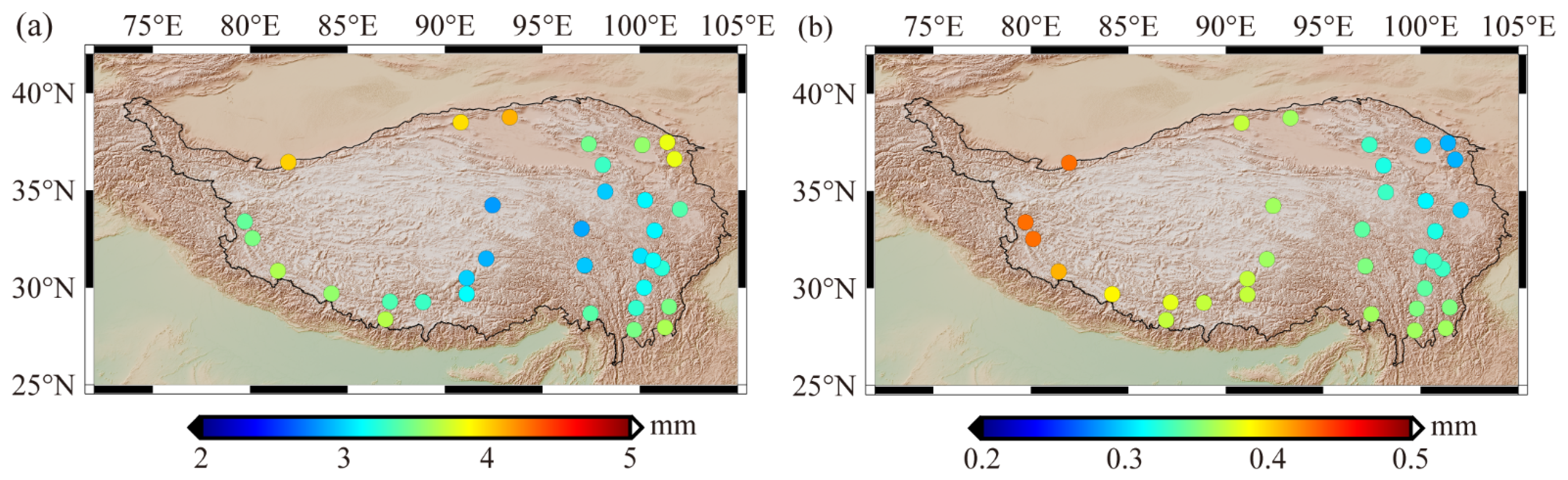
| Time Series | Linear Trend (mm·Year−1) | Annual Amplitude (mm) | Annual Phase (°) |
|---|---|---|---|
| 0.08 ± 0.01 | 2.32 ± 0.06 | 230.48 ± 0.03 | |
| 0.29 ± 0.02 | 2.12 ± 0.12 | 73.71 ± 0.06 | |
| 0.12 ± 0.01 | 1.73 ± 0.04 | 39.79 ± 0.02 | |
| 0.21 ± 0.02 | 4.34 ± 0.16 | 61.57 ± 0.04 | |
| 0.03 ± 0.01 | 4.03 ± 0.08 | 45.91 ± 0.02 |
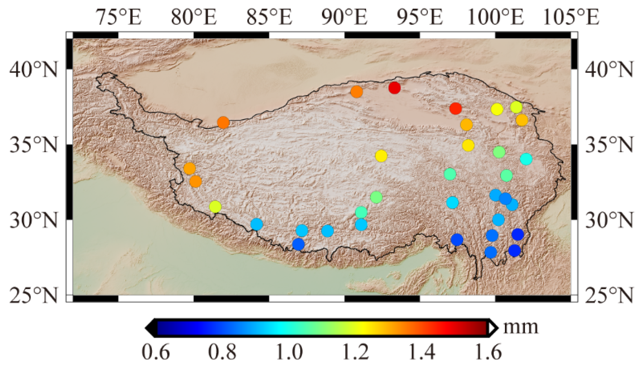
| Station | Lon. (°) | Lat. (°) | GPS Time Span (Year) | GPS (mm/Year) | SHF (mm/Year) | GF (mm/Year) |
|---|---|---|---|---|---|---|
| DLHA | 97.38 | 37.38 | 1999.16~2021.24 | 0.15 ± 0.04 | −0.20 ± 0.02 | −0.27 ± 0.01 |
| GSMA | 102.06 | 34.02 | 2010.67~2021.24 | 0.61 ± 0.16 | −0.24 ± 0.03 | −0.34 ± 0.02 |
| LHAS | 91.1 | 29.66 | 1999.16~2021.24 | 0.15 ± 0.08 | 0.76 ± 0.03 | 0.30 ± 0.02 |
| QHBM | 100.74 | 32.93 | 2010.88~2021.24 | 0.12 ± 0.13 | −0.09 ± 0.03 | −0.23 ± 0.02 |
| QHDL | 98.1 | 36.3 | 2010.65~2021.24 | 0.58 ± 0.20 | −0.23 ± 0.02 | −0.31 ± 0.01 |
| QHGC | 100.13 | 37.33 | 2011.01~2021.24 | 0.93 ± 0.16 | −0.16 ± 0.02 | −0.30 ± 0.01 |
| QHLH | 93.33 | 38.74 | 2010.72~2021.09 | 0.71 ± 0.18 | −0.12 ± 0.02 | −0.13 ± 0.01 |
| QHMD | 98.21 | 34.92 | 2011.18~2021.24 | 1.40 ± 0.19 | −0.13 ± 0.02 | −0.26 ± 0.02 |
| QHME | 101.4 | 37.47 | 2010.65~2021.24 | 1.62 ± 0.14 | −0.12 ± 0.02 | −0.29 ± 0.01 |
| QHMQ | 100.25 | 34.48 | 2010.64~2021.24 | 0.52 ± 0.17 | −0.09 ± 0.02 | 0.10 ± 0.01 |
| QHMY | 90.8 | 38.48 | 2011.44~2021.23 | 0.37 ± 0.16 | −0.07 ± 0.02 | −0.03 ± 0.01 |
| QHTT | 92.44 | 34.22 | 2011.25~2021.23 | 1.28 ± 0.15 | −0.01 ± 0.02 | 0.07 ± 0.01 |
| QHYS | 97.01 | 33.01 | 2010.66~2021.24 | −0.25 ± 0.19 | 0.07 ± 0.03 | −0.13 ± 0.02 |
| SCDF | 101.12 | 30.98 | 2011.01~2019.04 | 0.12 ± 0.18 | −0.12 ± 0.03 | −0.18 ± 0.02 |
| SCGZ | 100.02 | 31.61 | 2010.31~2021.24 | 0.15 ± 0.13 | −0.02 ± 0.03 | −0.17 ± 0.02 |
| SCJL | 101.5 | 29.01 | 2010.54~2021.23 | −0.48 ± 0.16 | −0.12 ± 0.03 | −0.15 ± 0.02 |
| SCLH | 100.67 | 31.39 | 2010.39~2021.24 | 0.37 ± 0.13 | −0.02 ± 0.03 | −0.17 ± 0.02 |
| SCLT | 100.22 | 29.99 | 2011.27~2021.24 | 0.61 ± 0.13 | 0.03 ± 0.03 | −0.09 ± 0.02 |
| SCML | 101.28 | 27.93 | 2010.50~2021.24 | −0.70 ± 0.21 | 0.08 ± 0.04 | −0.03 ± 0.03 |
| SCXC | 99.8 | 28.94 | 2010.55~2021.24 | −0.19 ± 0.14 | 0.15 ± 0.03 | −0.02 ± 0.03 |
| XJYT | 81.97 | 36.43 | 2011.13~2021.24 | −0.21 ± 0.14 | 0.07 ± 0.02 | −0.03 ± 0.01 |
| XNIN | 101.77 | 36.6 | 1999.16~2021.24 | −0.04 ± 0.06 | −0.19 ± 0.02 | −0.33 ± 0.02 |
| XZAR | 87.18 | 29.27 | 2011.27~2021.24 | −0.05 ± 0.20 | 0.59 ± 0.03 | 0.26 ± 0.02 |
| XZBG | 81.43 | 30.84 | 2011.25~2021.18 | 0.25 ± 0.23 | 1.18 ± 0.04 | 0.41 ± 0.03 |
| XZCD | 97.17 | 31.13 | 2010.33~2021.24 | 2.27 ± 0.20 | 0.39 ± 0.03 | 0.04 ± 0.02 |
| XZCY | 97.47 | 28.66 | 2010.68~2021.24 | 0.42 ± 0.23 | 0.43 ± 0.03 | 0.10 ± 0.03 |
| XZDX | 91.1 | 30.48 | 2011.09~2020.57 | 0.36 ± 0.16 | 0.66 ± 0.03 | 0.29 ± 0.02 |
| XZGE | 80.11 | 32.52 | 2010.94~2021.01 | 0.40 ± 0.20 | 0.92 ± 0.03 | 0.26 ± 0.02 |
| XZNQ | 92.11 | 31.49 | 2010.70~2013.41 | −0.00 ± 0.44 | 0.56 ± 0.03 | 0.27 ± 0.02 |
| XZRK | 88.87 | 29.25 | 2011.44~2021.24 | 0.91 ± 0.17 | 0.61 ± 0.03 | 0.26 ± 0.02 |
| XZRT | 79.72 | 33.39 | 2010.82~2021.24 | 0.47 ± 0.14 | 0.81 ± 0.03 | 0.17 ± 0.02 |
| XZZB | 84.16 | 29.68 | 2011.38~2019.91 | 1.15 ± 0.26 | 0.76 ± 0.04 | 0.33 ± 0.02 |
| XZZF | 86.94 | 28.36 | 2012.40~2021.24 | 0.63 ± 0.27 | 0.73 ± 0.04 | 0.30 ± 0.02 |
| YNZD | 99.7 | 27.82 | 2011.00~2021.22 | −0.72 ± 0.20 | 0.08 ± 0.04 | −0.03 ± 0.03 |
Publisher’s Note: MDPI stays neutral with regard to jurisdictional claims in published maps and institutional affiliations. |
© 2022 by the authors. Licensee MDPI, Basel, Switzerland. This article is an open access article distributed under the terms and conditions of the Creative Commons Attribution (CC BY) license (https://creativecommons.org/licenses/by/4.0/).
Share and Cite
Shi, T.; Guo, J.; Yan, H.; Chang, X.; Ji, B.; Liu, X. Assessing Height Variations in Qinghai-Tibet Plateau from Time-Varying Gravity Data and Hydrological Model. Remote Sens. 2022, 14, 4707. https://doi.org/10.3390/rs14194707
Shi T, Guo J, Yan H, Chang X, Ji B, Liu X. Assessing Height Variations in Qinghai-Tibet Plateau from Time-Varying Gravity Data and Hydrological Model. Remote Sensing. 2022; 14(19):4707. https://doi.org/10.3390/rs14194707
Chicago/Turabian StyleShi, Tong, Jinyun Guo, Haoming Yan, Xiaotao Chang, Bing Ji, and Xin Liu. 2022. "Assessing Height Variations in Qinghai-Tibet Plateau from Time-Varying Gravity Data and Hydrological Model" Remote Sensing 14, no. 19: 4707. https://doi.org/10.3390/rs14194707