
Analysis of the Anomalous Environmental Response to the 2022 Tonga Volcanic Eruption Based on GNSS
 ,
,  , ,
, ,
Abstract
:
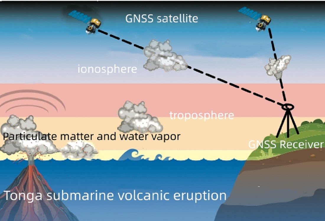
1. Introduction
2. Materials and Methods
2.1. Materials
2.2. Methodology
2.2.1. Zenith Non-Hydrostatic Delay Difference Calculation Method
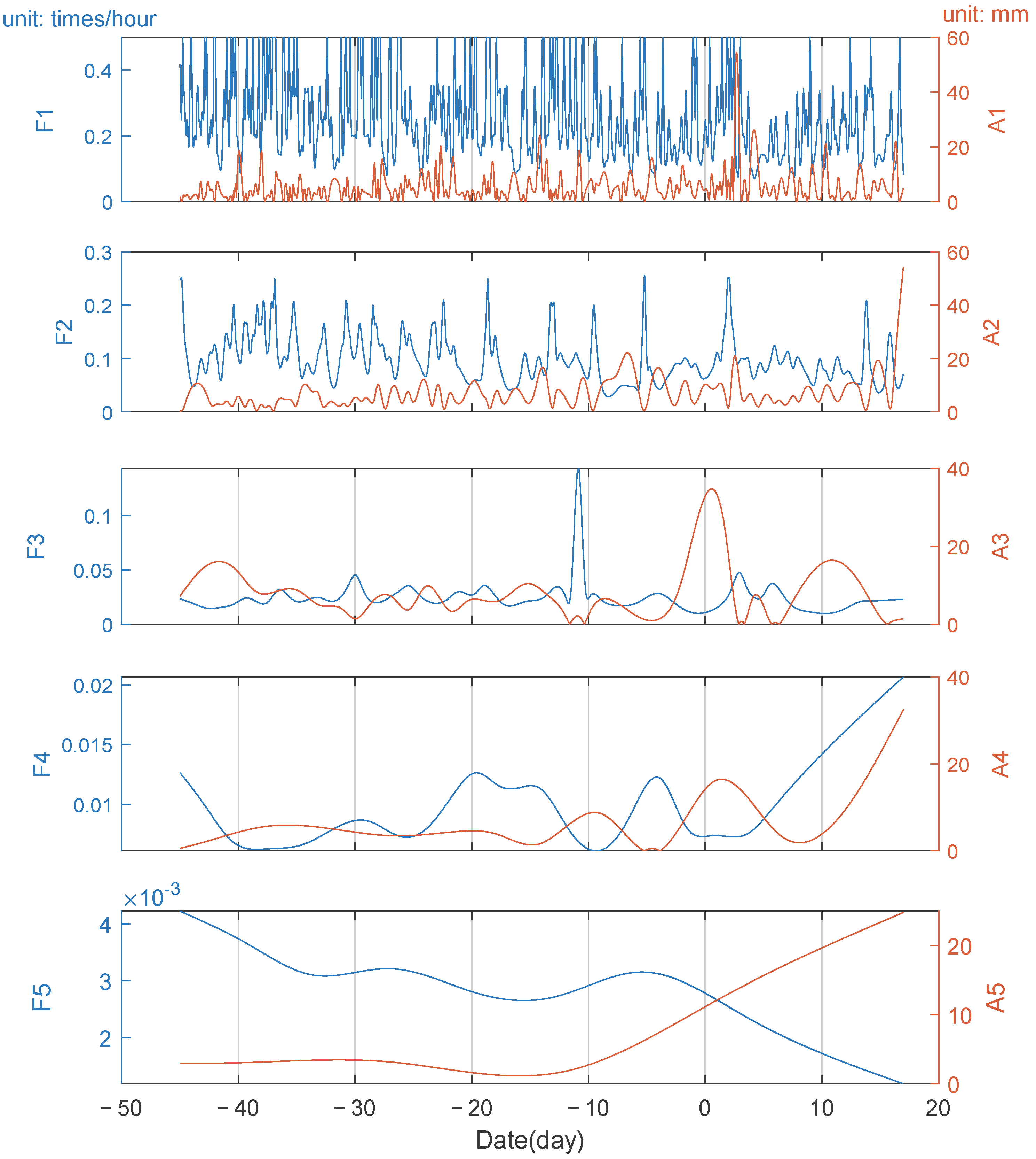
2.2.2. Extreme-Point Symmetric Mode Decomposition Method
- If , define and as the boundary maxima and minima, respectively.
- If (or ), then define and (or and ) as the boundary maxima and minima, respectively.
- If (or ), then define as the boundary minima (or minima) and use the line leading from the first minima to define the boundary minima (or minima). The magnitude of the slope here is determined by the left boundary point) and the line at the first extreme value point.
3. Results and Discussion
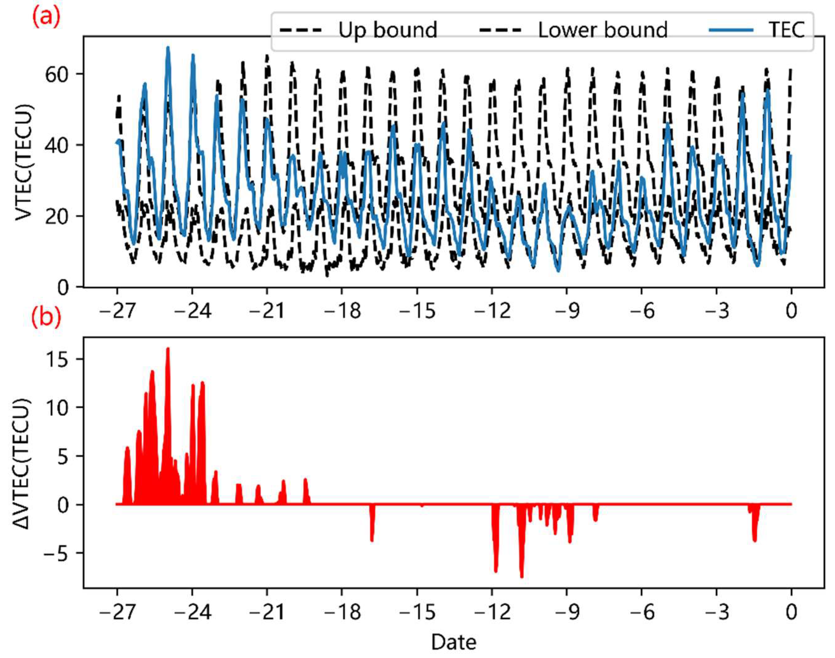
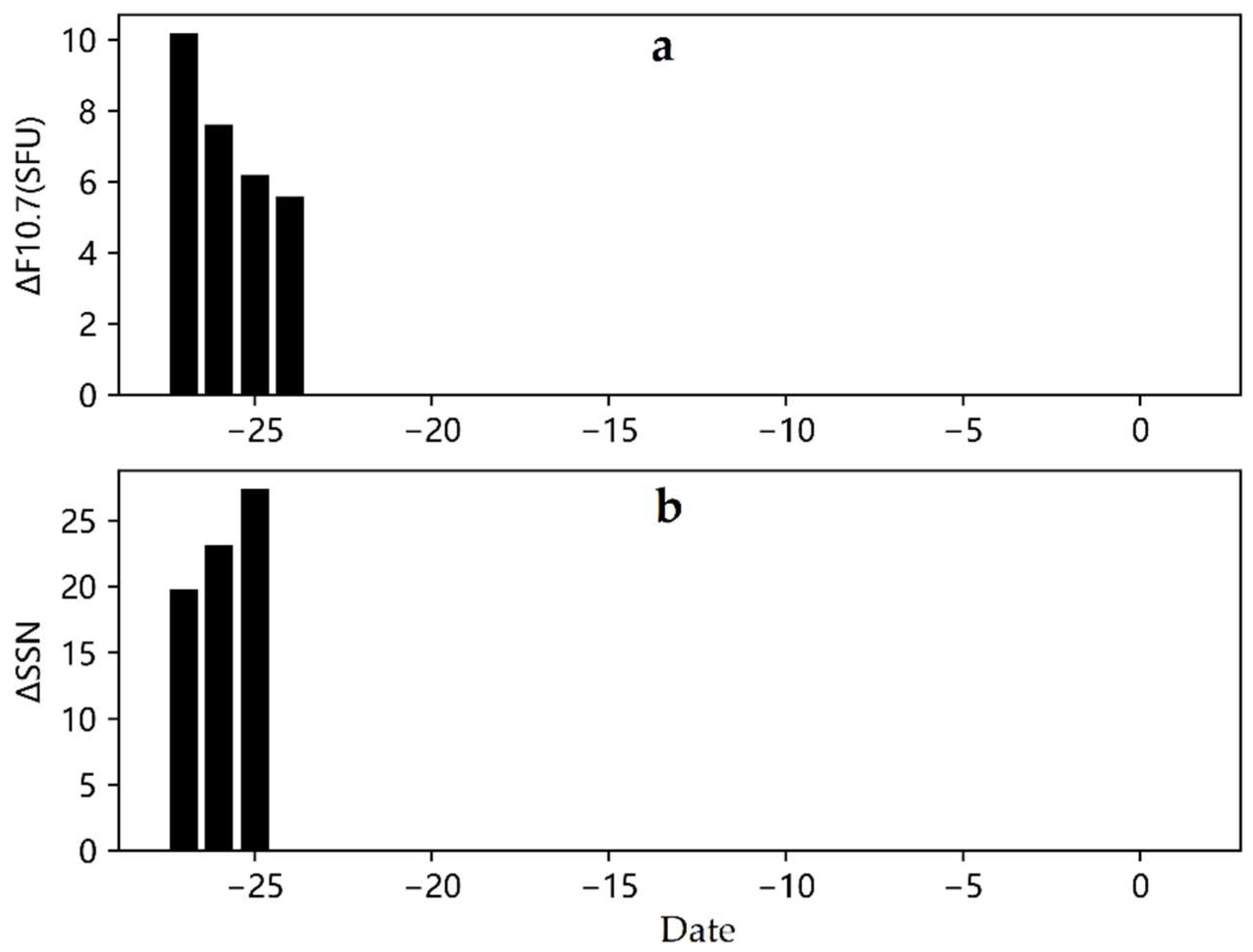
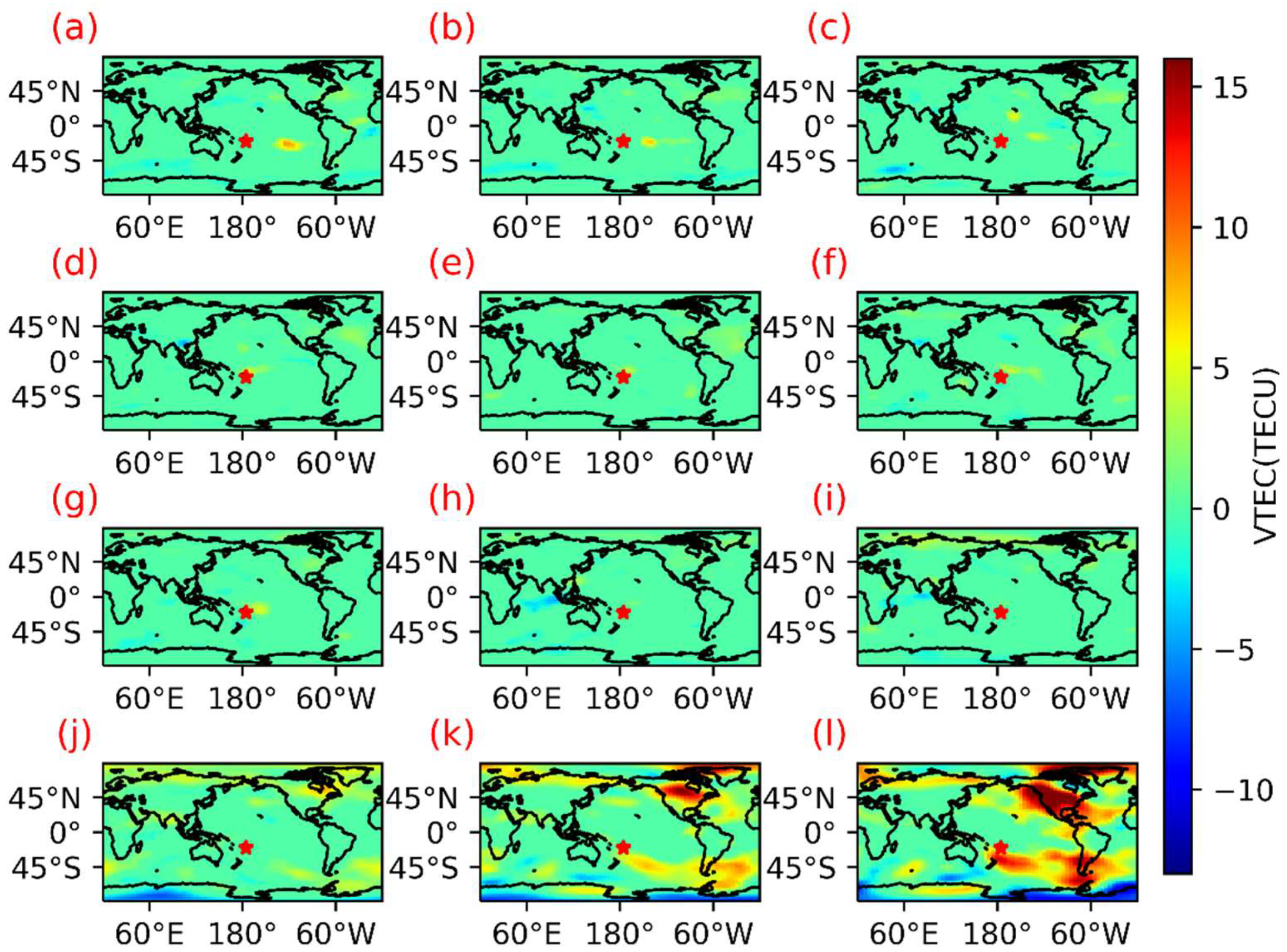
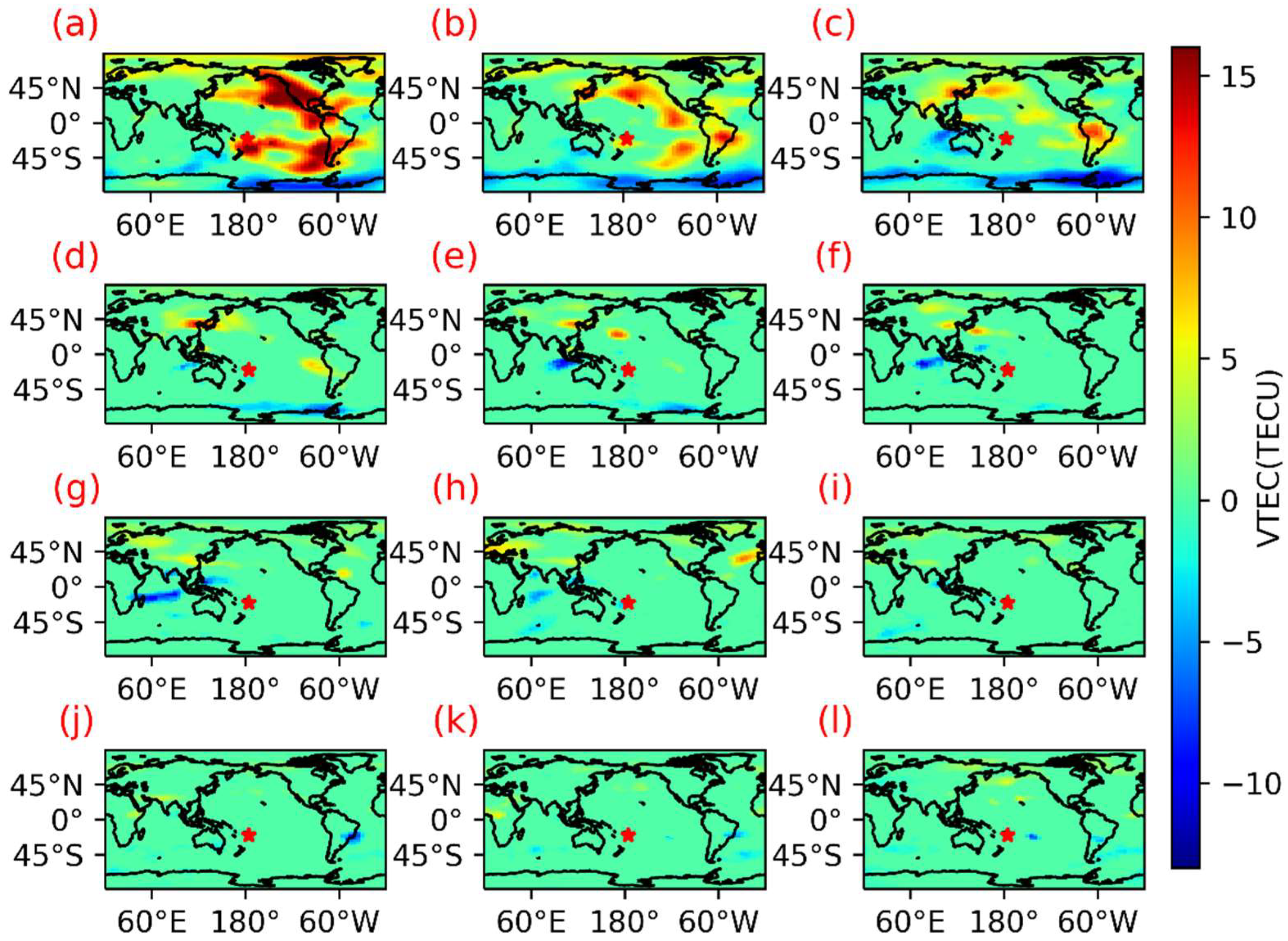
3.1. Analysis of Ionospheric Anomalies Prior to the Tonga Volcanic Eruption
- (1)
- Anomalous TEC disturbance detection prior to the Tonga volcanic eruption
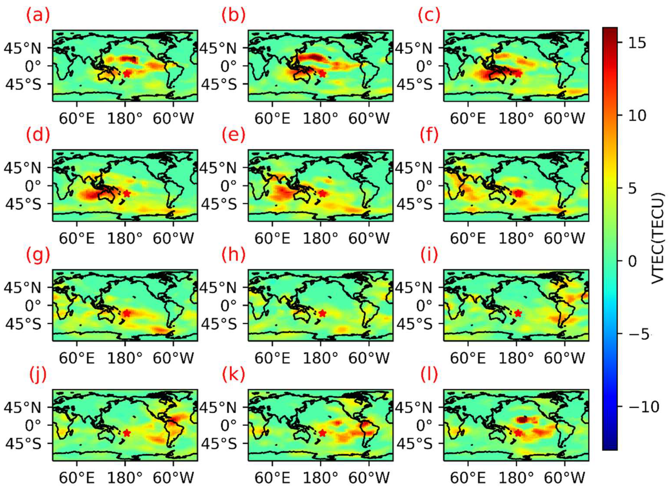
- (2)
- Global distribution of TEC anomalous disturbances
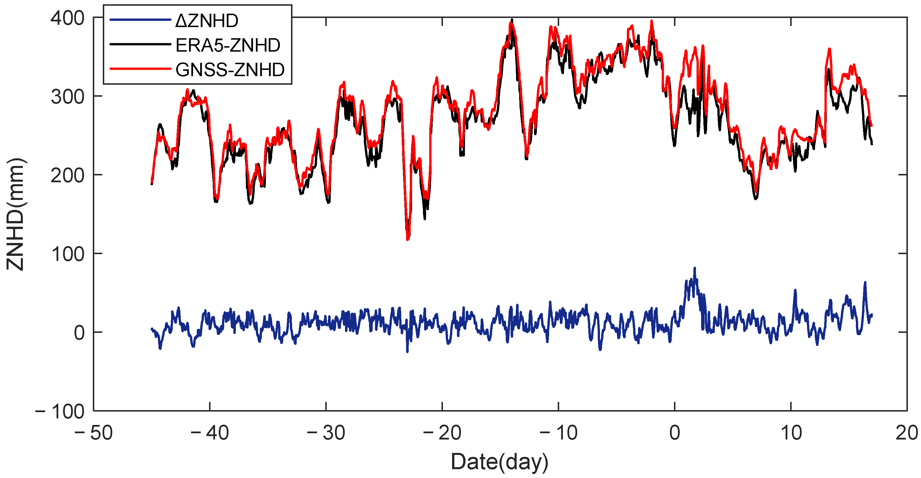
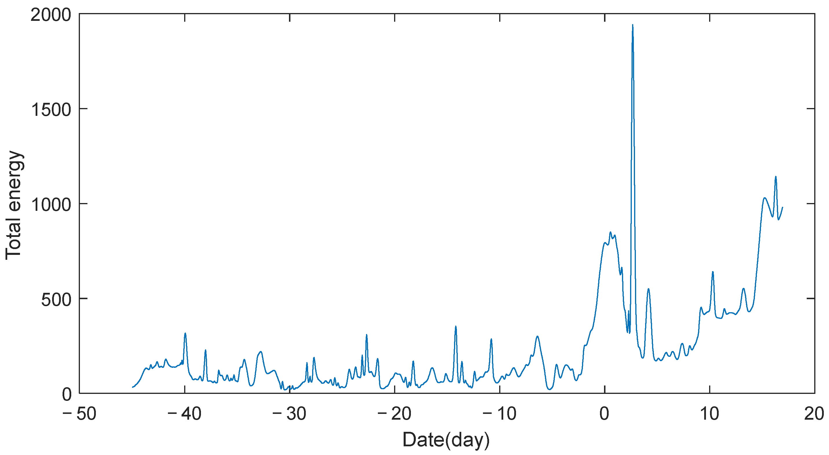
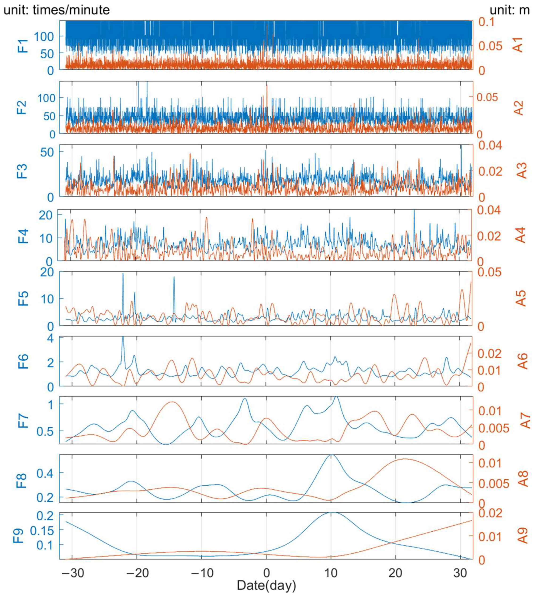
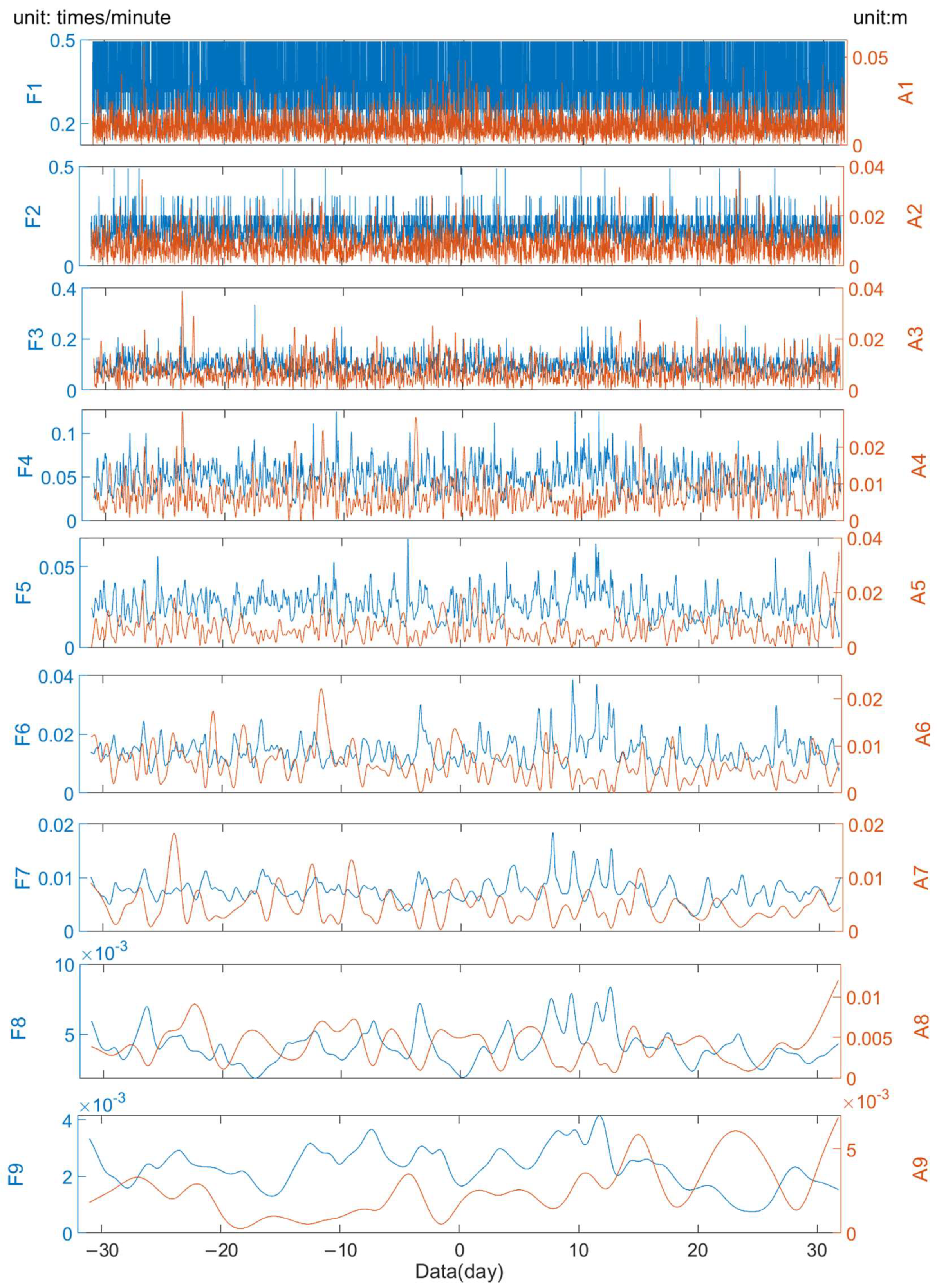
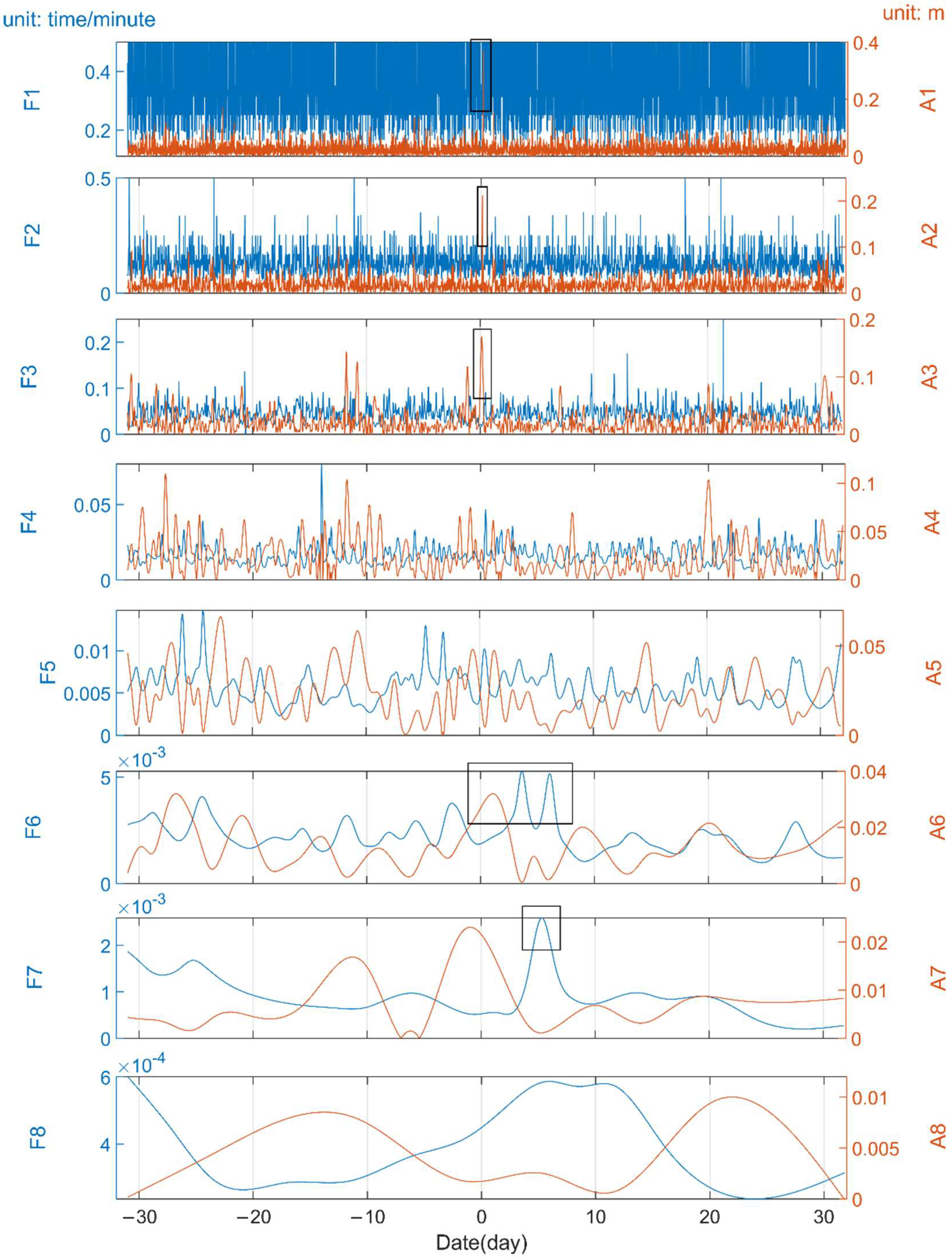
3.2. Analysis of Tropospheric Anomalies before and after the Tonga Volcanic Eruption
3.3. Influence of the HTHH Underwater Volcano Eruption on the Location of GNSS Station
4. Conclusions
Author Contributions
Funding
Data Availability Statement
Conflicts of Interest
References
- Themens, D.R.; Watson, C.; Žagar, N.; Vasylkevych, S.; Elvidge, S.; McCaffrey, A.; Prikryl, P.; Reid, B.; Wood, A.; Jayachandran, P.T. Global propagation of ionospheric disturbances associated with the 2022 Tonga volcanic eruption. Geophys. Res. Lett. 2022, 49, e2022GL098158. [Google Scholar] [CrossRef]
- Zhang, S.-R.; Vierinen, J.; Aa, E.; Goncharenko, L.P.; Erickson, P.J.; Rideout, W.; Coster, A.J.; Spicher, A. 2022 Tonga volcanic eruption induced global propagation of ionospheric disturbances via Lamb waves. Front. Astron. Space Sci. 2022, 9, 871275. [Google Scholar] [CrossRef]
- Klein, A. Volcano Eruption in Tonga Was a Once-in-a-Millennium Event. Available online: https://www.newscientist.com/article/2304822-volcano-eruption-in-tonga-was-a-once-in-a-millennium-event (accessed on 17 January 2022).
- Arculus, R. Deeply explosive. Nat. Geosci. 2011, 4, 737–738. [Google Scholar] [CrossRef]
- Pulinets, S.; Boyarchuk, K. Ionospheric Precursors of Earthquakes; Springer: Berlin, Germany, 2005. [Google Scholar]
- Leonard, R.; Barnes, R. Observation of ionospheric disturbances following the Alaska earthquake. J. Geophys. Res. 1965, 70, 1250–1253. [Google Scholar] [CrossRef]
- Sorokin, V.; Chmyrev, V.; Yaschenko, A. Electrodynamic model of the lower atmosphere and the ionosphere coupling. J. Atmos. Sol. Terr. Phys. 2001, 63, 1681–1691. [Google Scholar] [CrossRef]
- Hayakawa, M.; Molchanov, O.; Team, N. Achievements of NASDA’s earthquake remote sensing frontier project. Terr. Atmos. Ocean. Sci. 2004, 15, 311–327. [Google Scholar] [CrossRef]
- Guo, J.; Li, W.; Yu, H.; Liu, Z.; Kong, Q. Impending ionospheric anomaly preceding the Iquique MW 8.2 earthquake in Chile on 2014 April 1. Geophys. J. Int. 2015, 203, 1461–1470. [Google Scholar] [CrossRef]
- Li, W.; Yue, J.; Guo, J.; Yang, Y.; Zou, B.; Shen, Y.; Zhang, K. Statistical seismo-ionospheric precursors of M7. 0+ earthquakes in Circum-Pacific seismic belt by GPS TEC measurements. Adv. Space Res. 2018, 61, 1206–1219. [Google Scholar] [CrossRef]
- Guo, J.; Shi, K.; Liu, X.; Sun, Y.; Li, W.; Kong, Q. Singular spectrum analysis of ionospheric anomalies preceding great earthquakes: Case studies of Kaikoura and Fukushima earthquakes. J. Geodyn. 2019, 124, 1–13. [Google Scholar] [CrossRef]
- Shi, K.; Ding, H.; Guo, J.; Yu, T. Refined seismic-ionospheric effects: Case study of Mw 8.2 Chiapas earthquake on September 7, 2017. GPS Solut. 2021, 25, 87. [Google Scholar] [CrossRef]
- Li, Z.; Wang, N.; Li, M.; Zhou, K.; Yuan, Y.; Yuan, H. Evaluation and analysis of the global ionospheric TEC map in the frame of international GNSS services. Chin. J. Geophys. 2017, 60, 3718–3729. [Google Scholar] [CrossRef]
- Solheim, F.; Vivekanandan, J.; Ware, R.; Rocken, C. Propagation delays induced in GPS signals by dry air, water vapor, hydrometeors, and other particulates. J. Geophys. Res. Atmos. 1999, 104, 9663–9670. [Google Scholar] [CrossRef]
- Stoycheva, A.; Guerova, G. Study of fog in Bulgaria by using the GNSS tropospheric products and large-scale dynamic analysis. J. Atmos. Sol.-Terr. Phys. 2015, 133, 87–97. [Google Scholar] [CrossRef]
- Pun, V.; Tian, L.; Ho, K. Particulate matter from re-suspended mineral dust and emergency cause-specific respiratory hospitalizations in Hong Kong. Atmos. Environ. 2017, 165, 191–197. [Google Scholar] [CrossRef]
- Tang, X.; Hancock, C.M.; Xiang, Z.; Kong, Y.; de Ligt, H.; Shi, H.; Quaye-Ballard, J.A. Precipitable water vapour retrieval from GPS precise point positioning and NCEP CFSv2 dataset during typhoon events. Sensors 2018, 18, 3831. [Google Scholar] [CrossRef]
- Guo, J.; Hou, R.; Zhou, M.; Jin, X.; Li, C.; Liu, X.; Gao, H. Monitoring 2019 forest fires in southeastern australia with GNSS technique. Remote Sens. 2021, 13, 386. [Google Scholar] [CrossRef]
- Guo, J.; Hou, R.; Zhou, M.; Jin, X.; Li, G. Detection of particulate matter changes caused by 2020 California wildfires based on GNSS and radiosonde station. Remote Sens. 2021, 13, 4557. [Google Scholar] [CrossRef]
- Wallace, L.; Beavan, J.; Bannister, S.; Williams, C. Simultaneous long-term and short-term slow slip events at the Hikurangi subduction margin, New Zealand: Implications for processes that control slow slip event occurrence, duration, and migration. J. Geophys. Res. Solid Earth 2021, 117, 402–419. [Google Scholar] [CrossRef]
- Socquet, A.; Valdes, J.P.; Jara, J.; Cotton, F.; Walpersdorf, A.; Cotte, N.; Specht, S.; Ortega-Culaciati, F.; Carrizo, D.; Norabuena, E. An 8 month slow slip event triggers progressive nucleation of the 2014 Chile megathrust. Geophys. Res. Lett. 2017, 44, 4046–4053. [Google Scholar] [CrossRef]
- Chen, G.; Wu, Y.; Jiang, Z.; Liu, X.; Zhao, J. Characteristics of seismogenic model of MW9.0 earthquake in Tohoku, Japan reflected by GPS data. Chin. J. Geophys. 2013, 56, 848–856. (In Chinese) [Google Scholar] [CrossRef]
- Yue, H.; Lay, T. Inversion of high-rate (1 sps) GPS data for rupture process of the 11 March 2011 Tohoku earthquake (Mw 9.1). Geophys. Res. Lett. 2011, 38, L00G09. [Google Scholar] [CrossRef]
- Blewitt, G.; Hammond, W.; Kreemer, C. Harnessing the GPS data explosion for interdisciplinary science. Eos 2018, 99, 485. [Google Scholar] [CrossRef]
- Larson, K.; Levine, J. Carrier-phase time transfer. IEEE Trans. Ultrason. Ferroelectr. Freq. 1999, 46, 1001–1012. [Google Scholar] [CrossRef] [PubMed]
- Saastamoinen, J. Atmospheric correction for the troposphere and stratosphere in radio ranging satellites. Use Artif. Satell. Geod. 1972, 15, 247–251. [Google Scholar] [CrossRef]
- Hwang, C.; Peng, M.; Ning, J.; Luo, J.; Sui, C. Lake level variations in China from TOPEX/Poseidon altimetry: Data quality assessment and links to precipitation and ENSO. Geophys. J. Int. 2005, 161, 1–11. [Google Scholar] [CrossRef]
- Huang, N.E.; Shen, Z.; Long, S.R.; Wu, M.C.; Shih, H.H.; Zheng, Q.; Yen, N.-C.; Tung, C.C.; Liu, H.H. The empirical mode decomposition and the Hilbert spectrum for nonlinear and non-stationary time series analysis. Proc. R. Soc. Lond. Ser. A Math. Phys. Eng. Sci. 1998, 454, 903–995. [Google Scholar] [CrossRef]
- Wang, J.; Li, Z. Extreme-point symmetric mode decomposition method for data analysis. Adv. Adapt. Data Anal. 2003, 5, 1137. [Google Scholar] [CrossRef]
- Calais, E.; Minster, J.; Hofton, M.; Hedlin, M. Ionospheric signature of surface mine blasts from Global Positioning System measurements. Geophys. J. Int. 1998, 132, 191–202. [Google Scholar] [CrossRef] [Green Version]


| Parameter | Strategy |
|---|---|
| Software used | GipsyX Version 1.0 |
| Elevation angle cutoff | 7° |
| Mapping function | Vienna Mapping Function (VMF1) |
| Estimated frequency of tropospheric parameters | Zenith delay and gradients as random walk every 5 min |
| Ionosphere corrected | 1st order effect: Removed by LC and PC combinations 2nd order effect: Modeled using IONEX data with IGRF12 |
| Solid earth tide and pole tide | IERS 2010 Conventions |
| Ocean tide loading | FES2004 |
| Earth orientation parameter (EOP) model | IERS 2010 Conventions for diurnal, semidiurnal, and long period tidal effects on polar motion and UT1 |
| Index | Max | Min | Mean | Std | |
|---|---|---|---|---|---|
| Coordinate | E | 22.3 | 5.5 | 8.1 | 2.1 |
| N | 26.9 | 6.6 | 9.7 | 2.5 | |
| U | 55.1 | 20.8 | 25.8 | 7.9 | |
| Troposphere | ZTD | 3.30 | 1.70 | 2.21 | 0.26 |
| PWV | 0.53 | 0.28 | 0.36 | 0.04 | |
Publisher’s Note: MDPI stays neutral with regard to jurisdictional claims in published maps and institutional affiliations. |
© 2022 by the authors. Licensee MDPI, Basel, Switzerland. This article is an open access article distributed under the terms and conditions of the Creative Commons Attribution (CC BY) license (https://creativecommons.org/licenses/by/4.0/).
Share and Cite
Zhou, M.; Gao, H.; Yu, D.; Guo, J.; Zhu, L.; Yang, L.; Pan, S. Analysis of the Anomalous Environmental Response to the 2022 Tonga Volcanic Eruption Based on GNSS. Remote Sens. 2022, 14, 4847. https://doi.org/10.3390/rs14194847
Zhou M, Gao H, Yu D, Guo J, Zhu L, Yang L, Pan S. Analysis of the Anomalous Environmental Response to the 2022 Tonga Volcanic Eruption Based on GNSS. Remote Sensing. 2022; 14(19):4847. https://doi.org/10.3390/rs14194847
Chicago/Turabian StyleZhou, Maosheng, Hao Gao, Dingfeng Yu, Jinyun Guo, Lin Zhu, Lei Yang, and Shunqi Pan. 2022. "Analysis of the Anomalous Environmental Response to the 2022 Tonga Volcanic Eruption Based on GNSS" Remote Sensing 14, no. 19: 4847. https://doi.org/10.3390/rs14194847