An Automatic Individual Tree 3D Change Detection Method for Allometric Parameters Estimation in Mixed Uneven-Aged Forest Stands from ALS Data

Abstract

Forests play a central role in the management of the Earth’s climate. Airborne laser scanning (ALS) technologies facilitate the monitoring of large and impassable areas and can be used to monitor the 3D structure of forests. While the ALS-based forest measures have been studied in depth, 3D change detection in forests is still a subject of little attention in the literature due to the challenges introduced by comparing point cloud pairs. In this study, we propose an innovative methodology to (i) automatically perform a 3D change detection of forests on an individual tree level; (ii) estimate tree parameters with allometric equations; and (iii) perform an assessment of the aboveground biomass (AGB) variation over time. The area in which the tests were carried out was hit by an ice storm that occurred in the time interval between the two LiDAR acquisitions; furthermore, field measurements were carried out and used to validate the results. The single-tree segmentation of the point clouds was automatically performed with a local maxima algorithm to detect the treetop, and a decision tree method to define the individual crowns around the local maxima. The multitemporal comparison of the point clouds was based on the identification of single trees, which were matched when there was a correlation between the position of the treetops. For each tree, the DBH (diameter at breast height) and the AGB were also estimated using allometric equations. The results are promising and allowed us to identify the uprooted trees and estimate that about 40% of the AGB of the area under examination had been destroyed, with an RMSE over the estimation ranging between 4% and 21% in four scenarios.

1. Introduction

Forests cover one-third of our planet and are a key component of the terrestrial carbon cycle, accounting for more than half of the annual carbon flux between the Earth’s surface and atmosphere and sequester 163 tons·ha⁻¹ of carbon per year [1]. Forest conservation and sustainable management are crucial for the Earth’s climate. Traditionally, carbon stock capacity measures are based on the relationship between aboveground biomass (AGB) and stored carbon. Quantifying the AGB of forests is also essential for forestry and ecological studies on ecosystems, slope stability, biodiversity, ecological niche, species distributions, and informing fire risk, among many others [2,3].

Traditionally, AGB is determined using the tree diameter at breast height (DBH) and the tree height through allometric equations [4].

Tree DBH and tree height are traditionally measured in field inventories [5]. However, AGB data are expected to be measured over extensive areas of the globe, especially for the carbon stock estimation. This requires field data from remote and inaccessible areas [4]. Today, many biomass measurements are estimated, more or less precisely, using remotely sensed data. In fact, in the last 20 years, the use of remote sensing for measuring and monitoring tree parameters has become more frequent [6,7]. Tree parameters such as tree height, tree DBH, crown radius, and AGB are derived with mathematical models from optical imagery, synthetic aperture radar (SAR), and Light detection and ranging (LiDAR). In this regard, LiDAR sensors mounted on aerial supports such as airplanes, helicopters, and unmanned aerial systems (UAS) are particularly suitable for forest measurement [8]. Indeed, the three-dimensional reconstruction of forests with LiDAR point clouds accurately describes the physical characteristics of the forest stand canopy over large areas [4,5].

Several methods for estimating biomass from LiDAR data have been developed and published continuously over the last few years with increasing complexity and various techniques. Two main strands can be distinguished from the latest studies on AGB computing from ALS data: empirical methods and modeling methods. The empirical approaches are based on the correlation between the physical characteristics of forest stands (forest structure) and biomass. Such correlations are generally described by regressions with different degrees of complexity. Physical attributes may be regressed against either tree DBH or biomass to obtain general LiDAR-biomass models [6]. The allometric relations between biomass and LiDAR-derived measures may be defined by linear [9] and multiparameter equations [3,10,11], or may have stochastic relationships described by machine learning models [12,13]. Regardless of how complex the relationship between the input parameters (independent regression variables) and biomass is, empirical methods require data from in situ biomass samples as the dependent variable [12]. The sample data are then used to compute and calibrate the model. Among the advantages of empirical models is the low cost of calculation and ease of application. Still, they are restricted to specific forest types and geographical areas (i.e., site-specific) [6,12,14].

More recently, AGB quantification procedures have shifted away from the regression between LiDAR-derived characteristics and biomass measurements and increasingly include automated tree top detection and 3D computer vision [8]. Such modeling methods are based on the computer reconstructions of volumes and geometries based on LiDAR-derived point clouds. Modeling methods typically operate at an individual-tree scale and are applied in both mobile laser scanning (MLS) and ALS data [15,16,17]. Therefore, they require much higher density LiDAR point clouds and higher computational power than those needed by empirical models. On the other hand, modeling methods do not involve field data and are not site-specific. However, particular parameterizations based on the structure of the forests and the shape of the crown (generally related to conifers-broadleaves) are necessary. Frequently, the data retrieved from 3D modeling are then used as inputs in allometric formulas of general value, not site-specific, for the computation of forest metrics. This approach is particularly suitable for point clouds not associated with an in-the-field dataset as it happens, for example, in data collected on extensive areas such as surveys carried out by administrative bodies at the national and regional levels [2,12].

One of the main limitations of both the empirical and modeling models is reproducibility over large areas, which is seldom validated. This limitation is exacerbated in multitemporal analysis. In fact, while the estimation of forest parameters with LiDAR instruments has been studied in depth, 3D change detection in forests is still a subject of little attention in the literature due to the challenges introduced by comparing point cloud pairs [18,19]. Some attempts have been made in urban vegetation crown shape changes [15] and forest environments [19,20], focusing on the crown height model detection of cuts [21,22,23]. The study by [18] identified three main problems related to the 3D change detection: (i) the point cloud density; (ii) irregular sampling of point clouds; and (iii) irregular structure of tree crowns. For these reasons, performing a point-to-point comparison between the two epochs is impossible. They found a possible solution by performing the multitemporal analysis on the parameters estimated from the LiDAR data at a plot level instead of directly comparing the point clouds. The tree parameter-based change detection solution is only as good as the input data and the parameters estimation method. In 3D multitemporal analyses, there is a risk of bias induced by the procedure applied for the tree parameter estimation. However, the solution proposed in [18] allows for the automation of change detection, which in 3D forest is still an unexplored topic. Indeed, by automatically extracting forest parameters at individual tree scale from clouds of different epochs, which have to be co-registered, then the two clouds can be compared automatically.

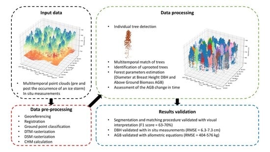
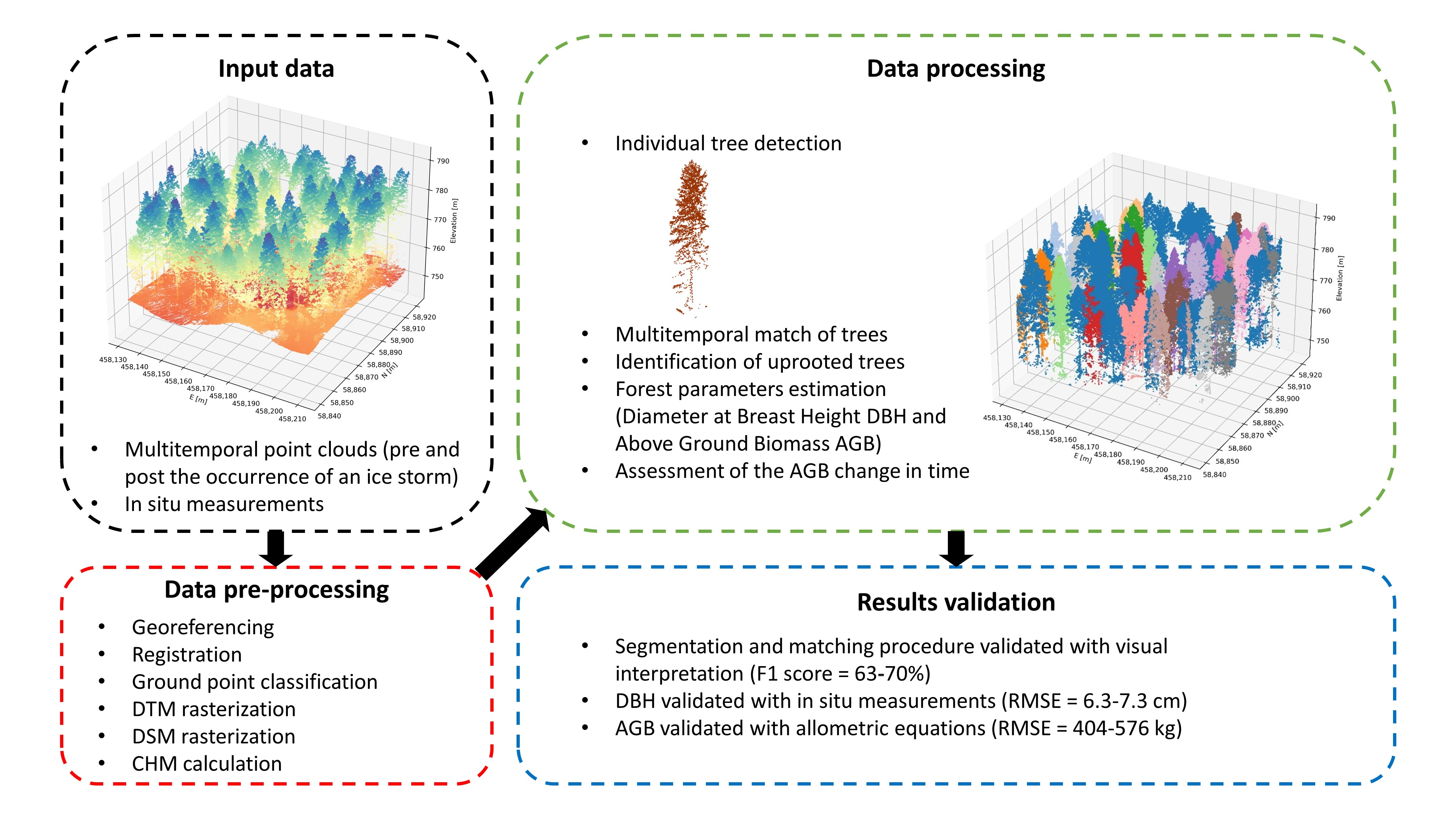
In this paper, we propose a methodology for the automatic 3D change detection of forests by defining the AGB at single-tree level from the airborne LiDAR point cloud. Moreover, we tested: (i) the accuracy of single tree segmentation procedures and allometric relations for the estimation of DBH, height, and crowns diameter; (ii) the role of the allometric variables in terms of error propagation for AGB and DBH estimations; and (iii) the assessment of the AGB changes over time.

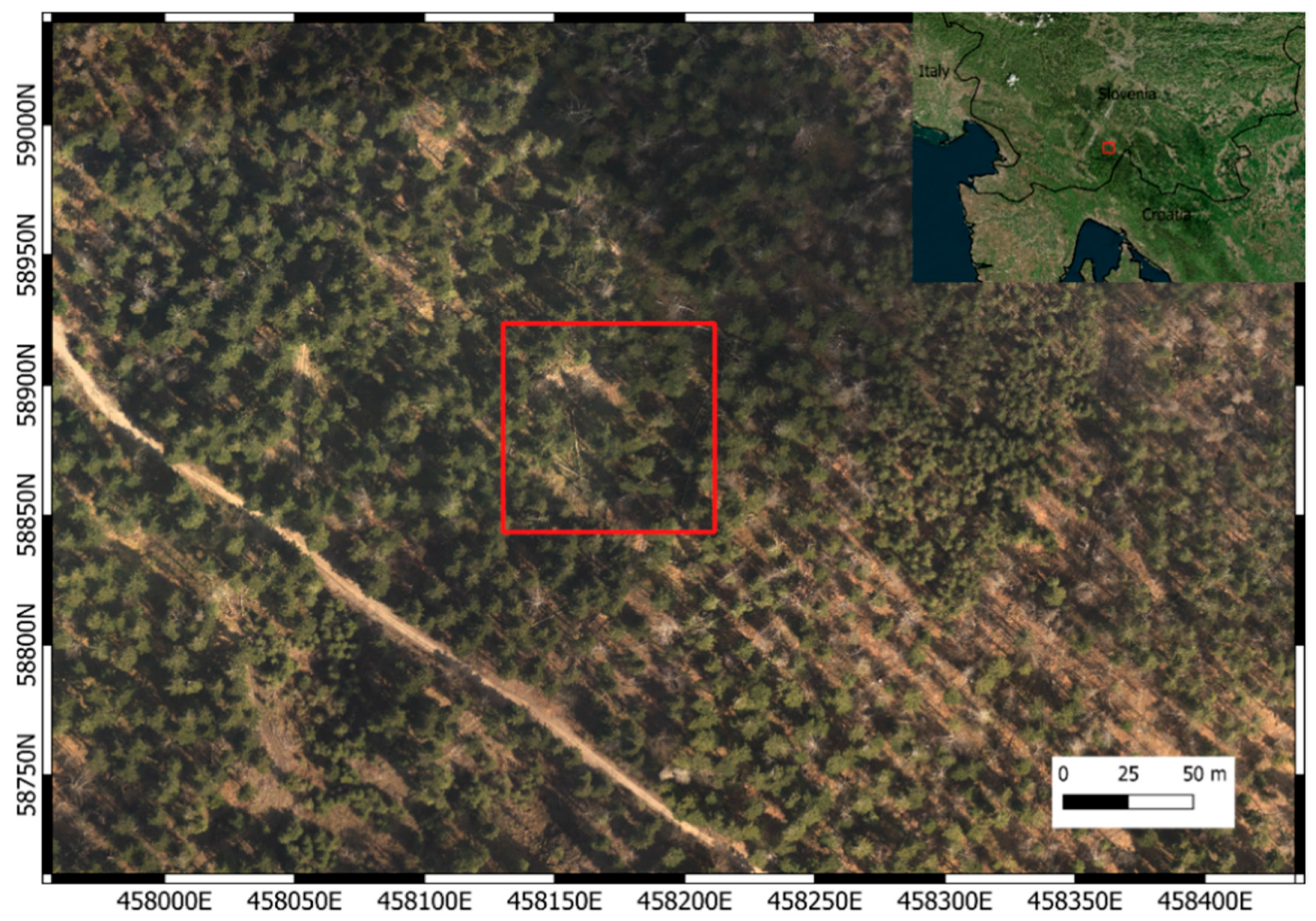
The tests were conducted in complex mixed uneven-aged forest stands in the Dinaric Mountains (SW Slovenia), where two ALS flights in 2013 and 2014 were flown. The forest stands were damaged by an ice storm in 2014. In this framework, the automatic AGB change detection has a bearing on the management of the disastrous effects of extreme natural events that have intensified in the study area, as in many other parts of the world, due to climate change.

2. Materials and Methods

2.1. Materials

In this study, we investigated an area located in the Dinaric Mountains in Southwest Slovenia (Figure 1).

The Dinaric silver fir—European beech forest is mainly made up of Silver fir (Abies alba Mill.), Norway spruce (Picea abies Karst.), and European beech (Fagus sylvatica L.) tree species. In January–February 2014, an extreme ice storm caused damage to more than half a million hectares of forests across Slovenia including the area considered as a case study. [24] As part of a Life+ ManFor C.BD. project, LiDAR acquisitions and in situ measurements were collected during November 2013 (pre-ice storm) and April 2014 (post-ice storm). The investigated area extended for about 4000 m² (35.7 m radius). In this area, two in situ campaigns were carried out: the first survey of trees (DBH ≥10 cm) was conducted in November 2013, and information about (i) tree locations (x and y coordinates), (ii) tree DBH, and (iii) the social status (a measure of the height of a tree relative to the surrounding trees) of each tree were collected. The height of 20 trees was measured in order to obtain a local height curve to establish the relationship between DBH and height for the study area. During the second survey, which took place in April 2014, the trees that were uprooted or damaged were identified. Laser scans were both acquired with a helicopter equipped with a Riegl LM5600. The flying altitude was 700 m above ground level, and the average point cloud density was about 250 points per square meter. The area covered by laser scans was larger than the area investigated in situ, but for the purposes of the analysis described in this article, only a square area of approximately 6400 m² including the circular plot for the in-field survey was considered.

The in situ surveyed circular area was composed, in November 2013, of 72 trees: nine of these were European beech, while 63 were Silver fir (

Table A1. The parameters of the trees located in the study area (Dinaric Mountains, Southwest Slovenia).

Tree Parameters	Features	Value
DBH [cm]	Minimum	10.2 cm
	Maximum	65.9 cm
	Mean	38.6 cm
Tree height [m]	Minimum	7.4 m
	Maximum	33.5 m
	Mean	24.5 m
Biomass [kg]	Minimum	16 kg
	Maximum	956 kg
	Mean	2415 kg
Social status (%)	Dominant and codominant trees	73.6% (53 trees)
	Suppressed trees	26.4% (19 trees)
Tree species composition (%)	Silver fir	87.5% (63 trees)
	European beech	12.5% (9 trees)

in Appendix A).

2.2. Methods

The workflow of the data processing carried out is described below (Figure 2). After acquiring the data, the pre-processing and the segmentation procedures were carried out for both the laser scans; afterward, when analyzing the outcomes obtained in the segmentation process, a change detection procedure was carried out to identify the uprooted trees. On a single-tree level, the primary tree parameters (tree DBH, tree height, tree biomass) were estimated using allometric equations. Finally, the amount of aboveground biomass lost because of the ice storm was assessed. The main procedure was fully automatized and implemented in Python language; the outputs were validated by comparing them with the in situ measured data and with user-defined visual analysis.

2.2.1. Pre-Processing

The point clouds acquired with the ALS system were registered and georeferenced

Primarily, the cloth simulation filter CSF point cloud filtering algorithm [25] was used, which identifies and classifies the points of the cloud belonging to the ground, distinguishing them from the points that identify natural and artificial objects (trees, houses, etc.).

The points that describe the planimetry of the ground were used to obtain the digital terrain model (DTM) through a rasterization procedure. Similarly, using the unclassified point cloud, the digital surface model (DSM) raster was obtained. The rasterization procedure was carried out by implementing the Whiteboxtool Python library [26]. The resolution of the DTM and DSM was 5 cm.

Finally, the canopy height model (CHM) was calculated as the difference between the DSM and the DTM with the same resolution. The CHM is DSM minus the DTM, and for forest analysis applications, it is fundamental because it allows for the height of the trees to be quickly extracted [27].

2.2.2. Segmentation Phase

The single-tree segmentation was performed with the PyCrown Python library [27] for the two laser scans. This algorithm finds the local maxima within the rasterized CHM, designates them as treetops, and then uses a decision tree method to grow individual crowns around the local maxima [14]. In more detail, the spatial evolution of the tree points around the treetop is regulated by four user-defined thresholds (

Table A2. The Pycrown parameter description and settings for the segmentation algorithm.

Parameter	Description	Optimal Values
Minimum_Threshold_1	The neighboring pixel is higher than the seed height * 0.7	0.7
Minimum_Threshold_2	The neighboring pixel is higher than the mean height of the current crown * 0.55	0.55
Maximum_Threshold	The neighboring pixel is below seed height * 1.05	1.05
Crown_radius	Maximum distance to the seed of 10 m	7 m

) [28]. In this study, the optimal thresholds were identified iteratively, performing the segmentation several times and evaluating the quality of the results for each scenario. The best segmentation outputs were obtained by setting the threshold proposed by Zörner [28] and modifying only the maximum radius of the crown, which was reduced to 7 m.

For each tree, the points that describe its crowns, branches, and stem were inscribed within a 2D convex hull and were uniquely labeled. In this phase, for both acquisitions, we had information related to the position of the trees, the height of the treetops (it was assumed that it coincided with the seed position), the shape and the extension of the crown, and the segmented point clouds on a single-tree level. The estimate of the diameter of the crown was performed, assuming that the latter had a circular shape.

Finally, further segmentation of the ground points was carried out to exclude any outliers from the analysis.

2.2.3. Multitemporal Matching

Multitemporal analysis was carried out to identify the same trees over time; in this way, it was possible to evaluate the effects of the ice storm in terms of felled trees, identifying their position and allowing to consider, on a single-tree level, the volumetric variation of the trees that survived the event for long periods.

The methodology was based on the use of information relating to the position of the trees. This choice was motivated based on the reasonable assumption that the position of the treetops cannot change considerably over time if they are not subject to human intervention, if they are not subject to damage caused by natural hazards, or if the damage is minor (some broken branches). The algorithm for each treetop in the pre-event time-period automatically carried out a spatial search associating the treetop of the closest tree in the post-event time-period to it (Figure A1). In this way, it was possible to automatically identify the same tree in acquisitions made at different times.

To improve the reliability of the matching result, a maximum search radius was set as the variable according to the radius of the crown. Thus, it was possible to identify and even match damaged trees, trees that have undergone a deviation from their usual vertical growth without falling to the ground, or experiencing irreversible damage. Furthermore, the closest treetop was matched if several treetops were in the search area. In this way, any possible erroneous matching caused by errors in the segmentation procedure were excluded, and double counting was avoided. Finally, the same nomenclature was applied to the trees associated in this way to facilitate subsequent analysis. When the algorithm did not associate any treetop, it meant that it was not able to find any treetop in the post-event time-period that described the same trees shown in the pre-event time-period. In these cases, the tree was considered uprooted and absent after the ice storm.

2.2.4. Estimation of Tree Parameters

The diameter at breast height DBH [cm] estimate was performed using the formula proposed in [4], calibrated, and validated with a forest database consisting of more than one hundred thousand trees:

$$DB{H}_{pred}=0.557\ast {\left(H\ast CD\right)}^{0.809}\ast \exp \left[\frac{{0.056}^2}{2}\right]$$

(1)

where H [m] is the tree height, and CD [m] represents the crown diameter.

The aboveground biomass AGB [kg] calculation was carried out using two allometric formulas. The first formula was proposed by [4] and differs according to the type of tree (angiosperm and gymnosperm trees) as a function of the ${\alpha }_g$ and ${\beta }_g$ parameters as follows:

$$AG{B}_{pred}=\left(0.016+{\alpha }_g\right)\ast {\left(H\ast CD\right)}^{\left(2.013+{\beta }_g\right)}\ast \exp \left[\frac{{0.204}^2}{2}\right]$$

(2)

In the case of gymnosperm trees (of which the study area is characterized), following the calibration, the parameters were set as follows:

$${\alpha }_g=0.093$$

(3)

$${\beta }_g=-0.223$$

(4)

This formula is particularly useful for remote sensing applications in the forestry field, as the two variables can be easily identified with the methods described above.

The second formula used to estimate biomass was described in [29], and is valid in a generic way without any distinction related to the species of trees:

$$AG{B}_{est}=0.0673\ast {\left(\rho \ast {\mathrm{DBH}}^2\ast H\right)}^{0.976}$$

(5)

where $\rho$ [g/cm³] is the wood-specific gravity, and the $DBH$ [cm] is calculated with Equation (1). In this study, we considered a wood-specific gravity value equal to 0.525 as reported in [30] regarding a mean of values in the Europe region. Unlike the previous equation, Equation (5) is defined as a function of the variable which, contrary to the CD estimate, is easier to measure when an in situ survey is planned. However, with Equation (5), we estimated a variation of the biomass only as a function of the change in the height of the tree (due to the breaking of the treetop); any changes due to the loss of branches were not taken into consideration.

In relation to the biomass estimate, a change detection analysis was carried out by calculating the biomass lost in the study area due to the ice storm. To this end, we compared both the biomass linked to the felled trees and the portion of wood lost from trees that still survived the disastrous event. For this purpose, to the best of our knowledge, we applied Equations (2) and (5) to both the intact and damaged trees. These equations were developed for undamaged trees, but we assume that they could provide consistent results and provide a quantitative estimate of biomass loss with good approximation.

2.2.5. Validation Process

The validation was carried out considering the results obtained in the three processing phases: (i) single-tree segmentation; (ii) multitemporal matching; and (iii) the estimation of tree parameters. In addition, an evaluation of the error propagation in the allometric equations used to estimate the tree parameters was carried out.

The single-tree segmentation procedure was assessed by comparing the output of the automated algorithm with the ground truth. The ground truth was obtained by performing a user-depending manual segmentation while simultaneously visually analyzing the CHM, the point cloud, and the position of the trees acquired during the in situ measurement campaign.

The accuracy assessment was evaluated with the PA (Producer’s Accuracy), UA (User’s Accuracy), and F1 score parameters [31], related as follows:

$${\mathrm{Producer}}^{’}\mathrm{s} \mathrm{Accuracy} =\frac{Nr. of matches}{Reference Crowns}$$

(6)

$${\mathrm{User}}^{’}\mathrm{s} \mathrm{Accuracy}=\frac{Nr. of matches}{Defined Crowns}$$

(7)

$$\mathrm{F}1 score=\frac{2\ast PA\ast UA}{PA+UA}$$

(8)

where $Nr. of matches$ is the number of trees correctly segmented; $Reference Crowns$ is the number of trees detected by the algorithm; and $Defined Crowns$ is the actual number of trees.

The single-tree segmentation was positively considered when it was not affected by (i) simple omission; (ii) under-segmentation (two or more trees are segmented as a single tree); and (iii) over-segmentation (a single tree is subdivided into two or more trees) (Figure 3).

It should be noted that in the validation phase, the suppressed trees were not taken into consideration and were excluded from the actual number of trees. The reason for this choice is related to the segmentation method used: the local maxima algorithm is not able to identify the treetops that are dominated by taller adjacent trees, and therefore they cannot be identified.

The validation of the multitemporal identification and matching of trees was performed using the same evaluation parameter. In this case, $Nr. of matches$ defines the number of trees correctly identified in both the laser scanner acquisitions, $Reference Crowns$ is the number of matches determined by the algorithm, while $Defined Crowns$ represents the actual number of trees that have not been uprooted. Additionally, in this case, the ground truth was obtained by performing a user-depending manual matching of the point cloud; the validation of the results was then carried out for each year with respect to the manually segmented and matched point cloud.

To evaluate the reliability of the allometric equations, we decided to conduct an error propagation analysis to quantify the error in the tree parameter (DBH, AGB) assessment as an effect of incorrect input values of the dependent variables. The analyses were carried out by introducing an error bias in the estimated crown diameter in Equations (1) and (2), and in the DBH in Equation (5). It was decided to consider only the error in these variables and to ignore any errors in estimating the height of the trees, assuming that this was obtained with sufficient precision by the local maxima algorithm. The error was then evaluated in percentage terms in the AGB estimate (2) due to an error in the prediction of the CD of (i) 0.1 m, (ii) 0.2 m, (iii) 0.5 m, and (iv) 1 m. The same error bias was introduced to evaluate the allometric Equation (1). Finally, the same considerations were made in the allometric equation for the AGB estimate (5), considering a systematic error in the estimate of the DBH of (i) 1 cm, (ii) 5 cm, and (iii) 10 cm.

Finally, the validation of the tree parameters was performed. The DBH values, calculated as Equation (1), were compared with the field measurements for the surveyed trees. We performed two different estimates of the DBH with Equation (1): in Scenario 1, the dependent variables were estimated on the point cloud automatically segmented by the algorithm; in Scenario 2, the crown diameter parameter was calculated on the single-tree segmented point cloud user-defined.

The aboveground biomass was not evaluated during the in situ survey; in this case, we assumed as the ground truth the AGB calculated with Equation (5) in which we considered the DBH values measured in situ. The AGB estimate was performed with Equations (2) and (5). As in the case of the DBH estimate, for each formula, the variables used were both those obtained automatically (Scenario 3 with Equation (2) and Scenario 5 with Equation (5)) and those obtained with manual segmentation (Scenario 4 with Equation (2) and Scenario 6 with Equation (5)) (

Table 1. The validation procedure summary and scenario nomenclature.

Tree Parameter	Estimate	Name	Validation Values
DBH	Equation (1) (variables derived from automatic segmentation)	Scenario 1	In situ measurements
	Equation (1) (variables derived from manual segmentation)	Scenario 2
AGB	Equation (2) (variables derived from automatic segmentation)	Scenario 3	Equation (5) (with the DBH measured in situ)
	Equation (2) (variables derived from manual segmentation)	Scenario 4
	Equation (5) (variables derived from automatic segmentation)	Scenario 5
	Equation (5) (variables derived from manual segmentation)	Scenario 6

).

3. Results

3.1. Segmentation and Multitemporal Matching

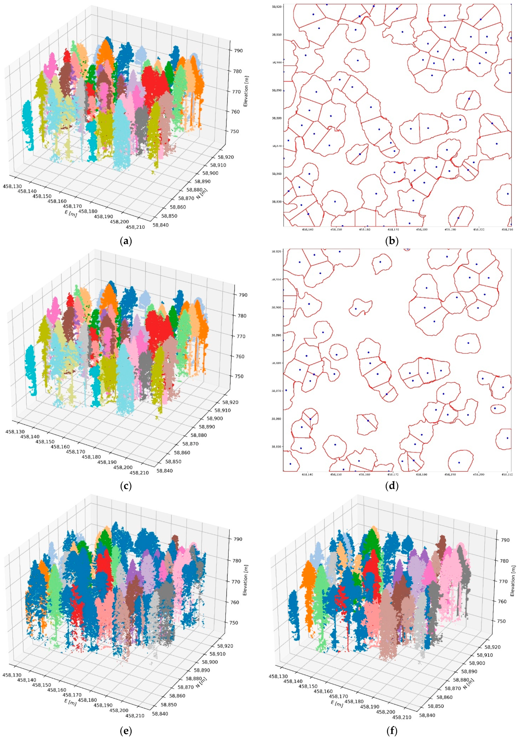
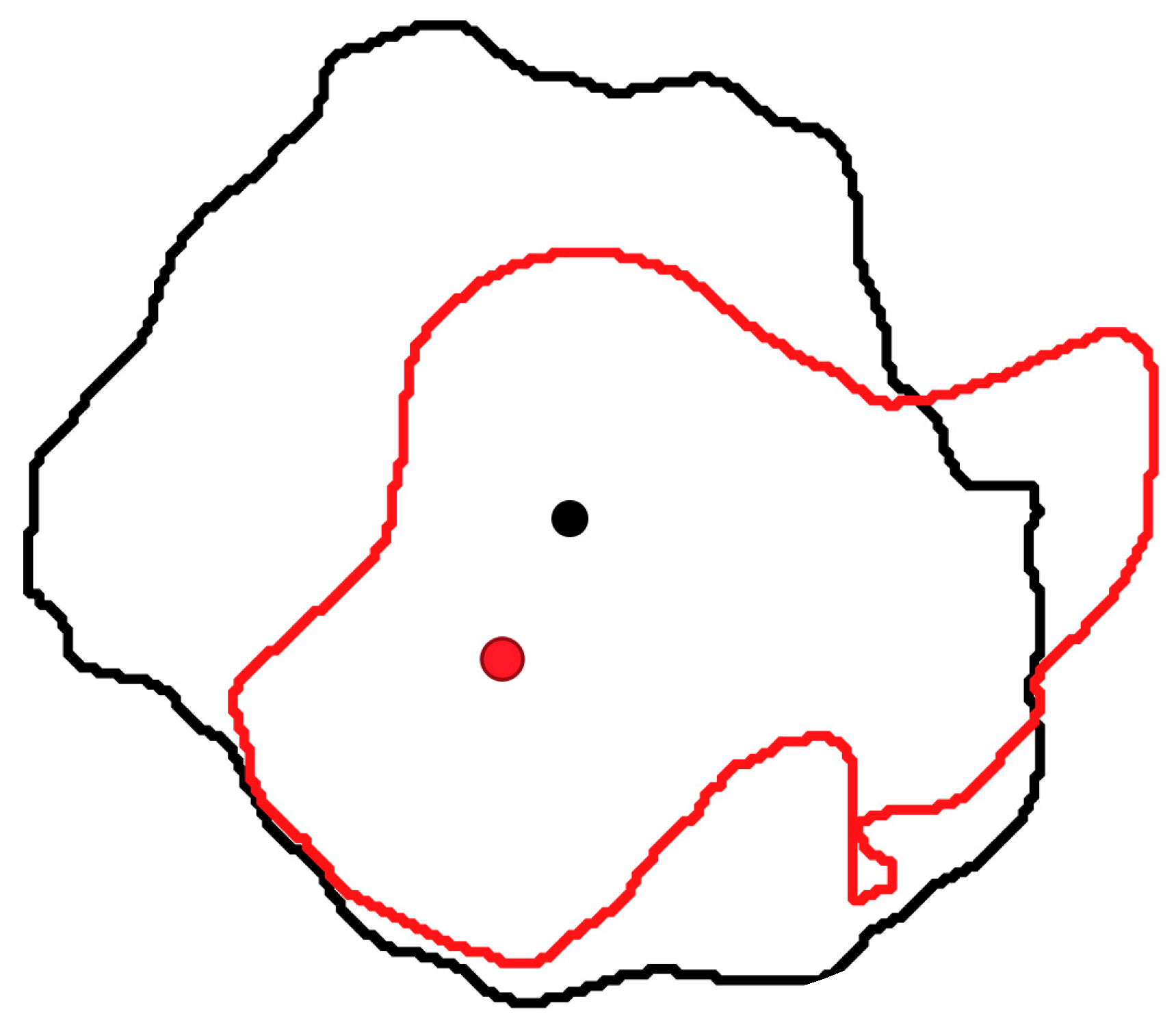
The results showed the reliability of the segmentation (Figure 4a–d) and matching procedures (Figure 4e,f). For most trees that survived the ice storm, a match was defined with a tree present before the storm (Figure 4f). Additionally, trees plotted in dark blue in the 2014 time period identified trees that were segmented incorrectly, causing a mismatch with the same tree in the 2013 time period.

Regarding the accuracy of the segmentation procedure, the F1 scores values were equal to 70% and 68% for the pre- and post-ice storm, respectively, and they showed high consistency with each other (

Table 2. The accuracy assessment of the single-tree segmentation procedure (on the left) and the multitemporal matching procedure (on the right). M = Matched Crowns; RC = Reference Crowns; PA = Producer Accuracy; DC = Defined Crowns; UA = User Accuracy.

Parameters	Segmentation Procedure		Multitemporal Matching Procedure
	2013	2014	2013	2014	Hypothetical Scenario
DC	79	58	42	42	42
RC	87	56	56	56	56
M	58	39	0.61	0.55	0.7
PA	0.67	0.7	34	31	39
UA	0.73	0.67	0.81	0.74	0.93
F1	70%	68%	69%	63%	80%

). With respect to the validation of the multitemporal matching and change analysis algorithm, the F1 score values settled at 69% in the pre-event scenario and 63% post-event (Table 2). It should be noted that these values cannot be higher than the F1 score values in the segmentation phase since it is not possible to correctly match trees that are not adequately detected simultaneously in the two acquisitions. To further test the reliability of the multitemporal association, it was decided to consider a hypothetical scenario in which we assumed that only during the point cloud segmentation procedure of the data acquired before the ice storm occurrence, no over-segmented trees were recorded. Under these conditions, the F1 score increased, and it reached a value of 80%.

3.2. Error Propagation in the Allometric Equations

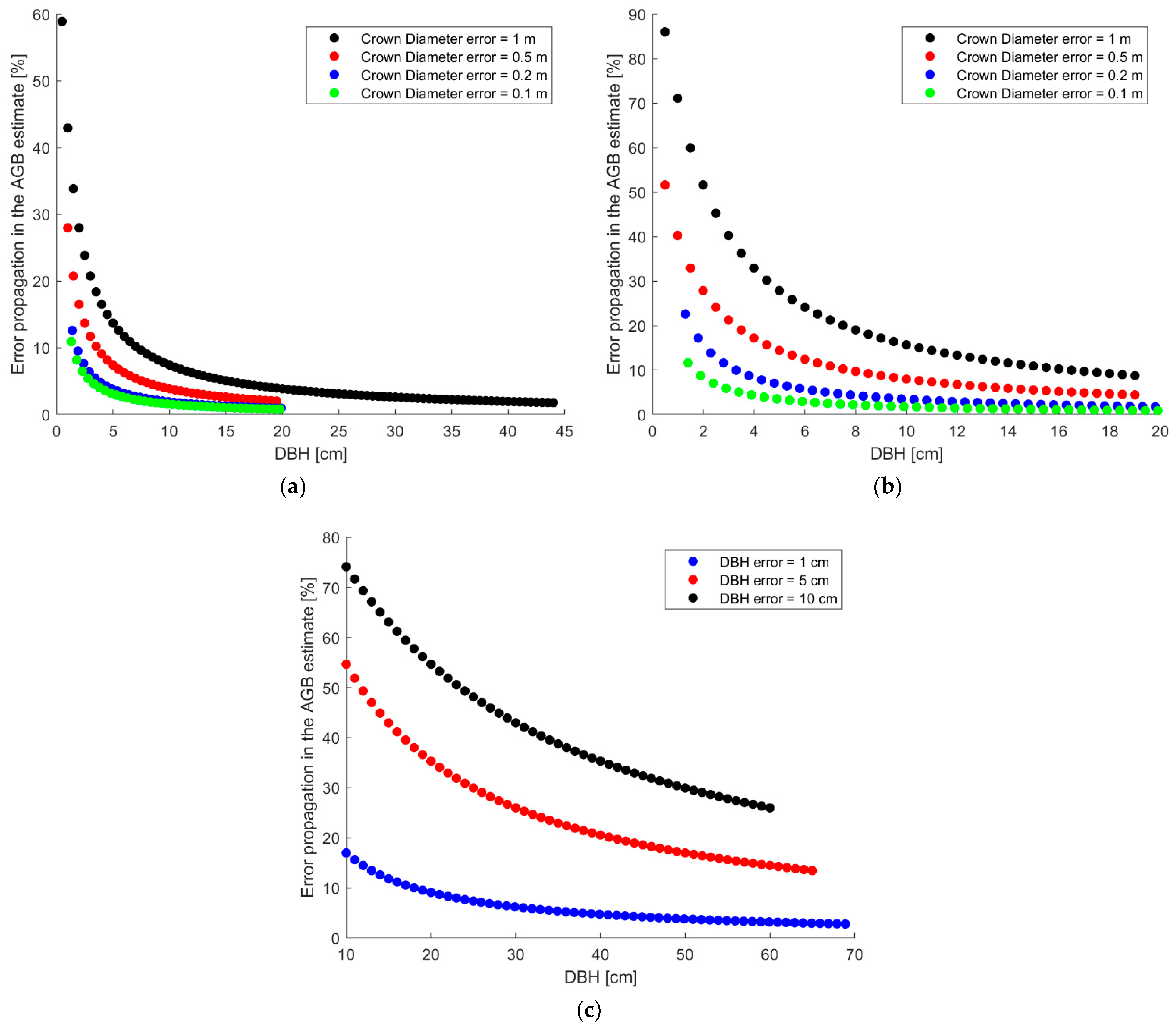
The results of the estimation of the error propagation of Equations (1), (2) and (5) are detailed below. All of the equations assumed an exponential trend in the percentage of error committed, and the propagation of the error in the estimation of the parameters increased as the size of the tree (crown diameter) decreased.

In reference to Equation (1), it was observed (Figure 5a) that the DBH estimate for trees with a crown described by a diameter between 5 and 14 m (such as those analyzed in the case in question) was affected by a maximum error propagation of about 15% when the error in the evaluation of the diameter of the canopy was one meter. Considering errors of this estimate of less than one meter, the percentage of the error committed was less than 10% for the trees in the study area.

When evaluating the error propagation in the AGB estimation through Equation (2), an error in the estimation of the crown diameter equal to one meter could lead to an overestimation of the biomass of the trees by up to 30%. The overestimation could be reduced and limited to 15% if the overestimation of the CD was halved (Figure 5b).

Equation (5) is affected by error propagation with the fastest exponential growth compared to the previous equations (Figure 5c), since the analyzed parameter (the DBH, expressed in centimeters) is squared. For the smallest trees (with DBH between 10 and 20 cm), an error in the estimate of 1 cm caused an error in terms of percentage ABG between 10 and 20%; if the DBH was overestimated by 10 cm, this error could exceed 70%. If we consider the medium/large trees, the percentage error of the ABG was reduced and became reasonable if the DBH was estimated with a maximum error of 1 cm, while it reached values higher than 15–20% for estimates affected by more significant uncertainty (5 cm).

3.3. Tree Parameters

The DBH and the AGB were estimated on the segmented trees. Greater attention was paid to trees for which a multitemporal matching between acquisitions was identified to evaluate the variation of parameters (the AGB) after the natural disaster occurred. Among these trees, those for which no in situ measurements were available (the surveyed area was smaller than the area acquired with the laser scanner) were further discarded.

The trees that had been correctly identified and matched in the overall area totaled 31. Overall, thirty-one trees were correctly identified and matched; of these, 15 were used to evaluate the accuracy of the assessments performed since they were located within the test area for in situ investigations and for which the DBH was measured.

The diameter estimation was carried out using the tree parameters (tree height and crown diameter) obtained from the point cloud acquired before the occurrence of the ice storm. In the case of trees that suffered damage (e.g., the crown had shrunk, the highest branches were broken), there was a risk of underestimating the diameter.

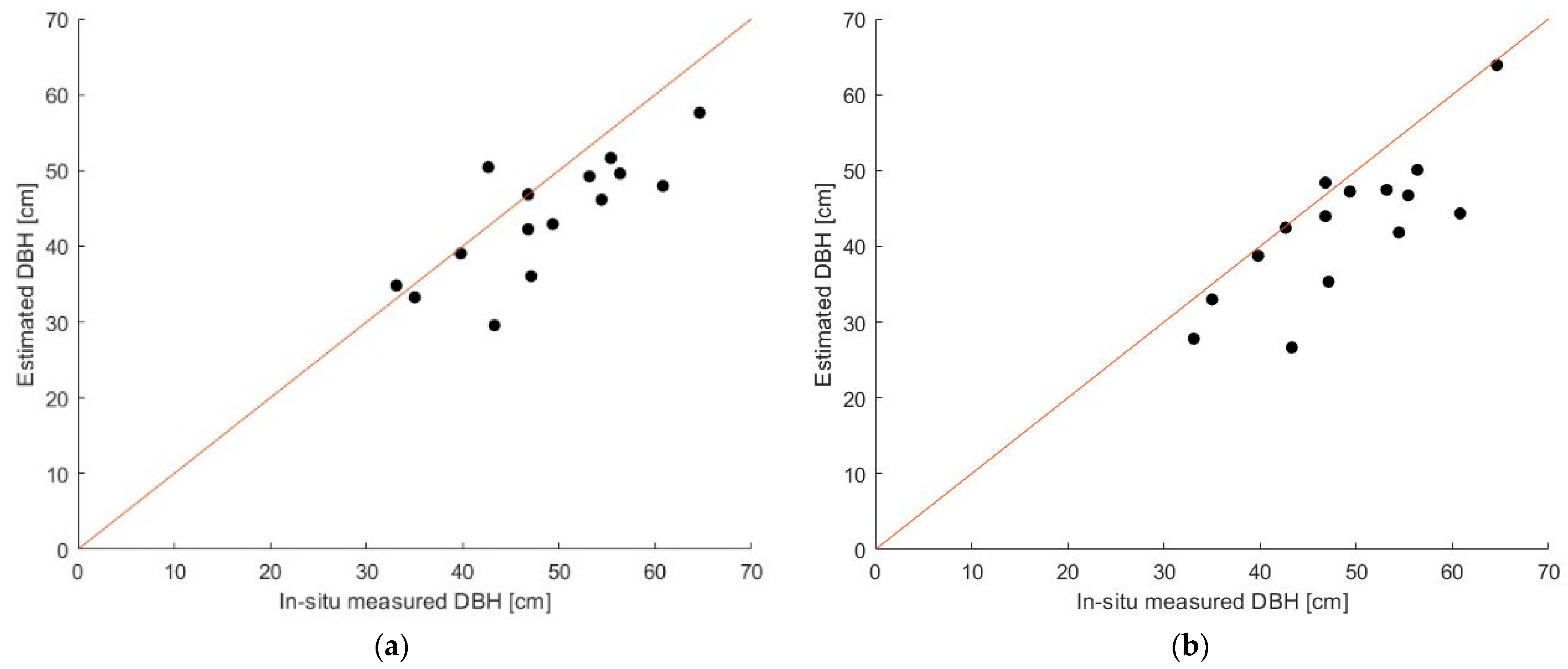
The scatter plots for the DBH estimated with Equation (1) considering Scenario 1 and Scenario 2 (Figure 6) showed a slight tendency to underestimate the DBH using the allometric equation, for which the bias was between about −9% and −12%, and the RMSE value was between 7.3 cm and 8.3 cm (

Table 3. The metric errors in the estimation of the DBH and AGB at the tree level in different scenarios.

Error Metrics	RMSE		Bias
Year	2013	2014	2013	2014
Scenario 1	7.3 cm	-	−9.00%	-
Scenario 2	8.3 cm	-	−12.30%	-
Scenario 3	404 kg	581 kg	−4.5%	−24.0%
Scenario 4	495 kg	438 kg	−9.7%	−14.9%
Scenario 5	532 kg	495 kg	−15.5%	−15.5%
Scenario 6	576 kg	570 kg	−21.3%	−21.7%

).

The results in the error metrics showed a lower RMSE and a lower bias when estimating the DBH considering the crown diameter as an output of the automatic single-tree segmentation; In contrast, manual segmentation led to values with a more significant average error and greater variability. In both scenarios, it was observed that Equation (1) seems to lead to underestimating the actual size of the DBH, providing errors up to the order of magnitude of the decimeter. Trees for which the diameter estimate performed the worst were mainly located in particularly dense areas in which the crowns of the trees intersected each other, and the extension of the canopy was not easily identifiable. In the sparser areas, the errors were considerably lower.

The tree biomass assessment was carried out with Equations (2) and (5) according to Scenario 3, Scenario 4, Scenario 5, and Scenario 6 and compared with the estimated ground truth as described in Section 2.2.5; finally, the metric errors (RMSE and bias) were calculated (Table 3). The minimum, maximum, and average AGB for each scenario was also calculated (

Table 4. The AGB estimate at the tree level: the minimum, maximum, and mean values in different scenarios.

Scenario	Features	AGB 2013 [kg]	AGB 2014 [kg]
Scenario 3	Minimum	726	356
	Maximum	3573	2492
	Mean	1783	1265
Scenario 4	Minimum	573	414
	Maximum	4002	3137
	Mean	1795	1449
Scenario 5	Minimum	573	524
	Maximum	3497	3244
	Mean	1655	1434
Scenario 6	Minimum	432	347
	Maximum	3655	3254
	Mean	1647	1416
Validation values	Minimum	606	487
	Maximum	3734	3025
	Mean	1975	1679

)

The metrics (Table 3) highlight that all of the scenarios considered (Scenario 3, Scenario 4, Scenario 5, and Scenario 6) tend to underestimate the tree AGB with a minimum average percentage of −4.5% and a maximum average percentage of −21.3%. The biomass estimates in the 2014 scenario were, on average, worse when compared to the biomass estimated of the same trees before the natural hazard, both with respect to the RMSE and the bias values.

After having estimated the tree parameters, it was possible to assess the biomass lost in the area under investigation due to the ice storm. At first, we decided to calculate the biomass lost only from the trees that had been correctly segmented and matched in the two multitemporal point clouds. The results (

Table 5. The biomass loss estimates of the matched trees, surviving trees, and the complete area in the study area in different scenarios.

Biomass Loss	Matched Trees		Surviving Trees		Total
	[kg]	[%]	[kg]	[%]	[kg]	[%]
Scenario 3	7727 kg	29.4%	14,500 kg	29.0%	51,352 kg	42.4%
Scenario 4	4916 kg	19.0%	9688 kg	19.3%	56,377 kg	39.7%
Scenario 5	3838 kg	15.8%	6176 kg	13.3%	50,382 kg	45.3%
Scenario 6	4129 kg	17.6%	6467 kg	14.0%	59,287 kg	44.3%
Ground truth	4430 kg	15.0%	-	-	-	-

) quantify the ground truth AGB loss of these trees as about 4430 kg (about 15% of their total biomass). The estimates resulting from the four scenarios are in line with this quantity, except for Scenario 3, according to which the biomass lost by the matched trees was greater and approximately equal to 29.4%. The scenarios that provided the best results were Scenario 5 and Scenario 6, where Equation (2) was applied.

To the aim of the assessment described above, however, trees that were correctly matched but for which we did not have the in situ measured DBH were excluded. When considering all the trees that survived the hazard (Table 5), it was shown that the biomass assessment was consistent for all the scenarios, with one considering only matched trees.

Additionally, to account for trees that survived the storm but which were not correctly identified and matched in both acquisitions, we believe that it is necessary to apply a correction factor that increases the amount of biomass estimate loss by about 30%. This percentage was chosen because about 30% of the surviving trees were not correctly multitemporally matched (Table 2).

Finally, considering the biomass of all of the segmented trees, the estimates were similar to each other, identifying about 40% of the AGB lost due to the ice storm (Table 5).

4. Discussion

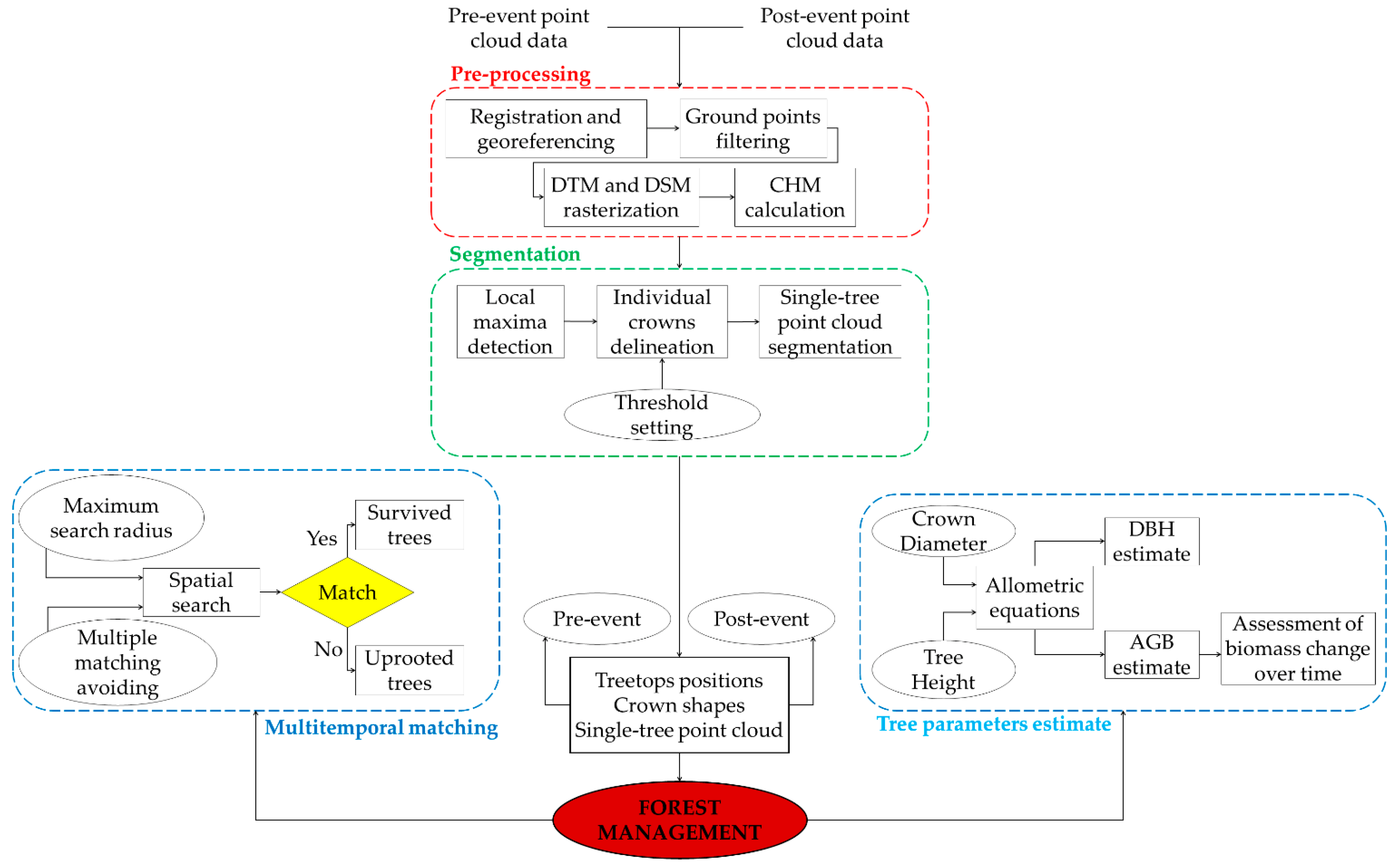
The results of this very first application of the multitemporal analysis of airborne point clouds for the assessment of single tree parameters and the evaluation of their change over time are promising as they are characterized by good accuracies and low errors. In particular, the procedural methodology proposes a new approach for the multitemporal comparison of point clouds in forest environments subjected to strong changes due to natural hazards. The 3D change detection was performed by implementing a single-tree level segmentation algorithm, and subsequently compared the segmented point clouds using forest parameters (treetops and crown diameters); then, the estimation of DBH and AGB was carried out through the application of allometric formulas. Finally, the biomass variation was performed by comparing the AGB estimated before and after the ice storm. A further innovative aspect lies in the complete automation of the entire procedure, which provides the possibility of applying the algorithm to any forest scenario.

The accuracy obtained in the segmentation phase achieved excellent results, with an F1 score of about 70%. In detail, this value appeared to be consistent with those proposed in the literature and obtained with different techniques and algorithms [32,33]. In particular, ref. [32] analyzed how the heterogeneity and density of the investigated area affected the final performance of the segmentation. Moreover, the goodness of the results was in line with the accuracy proposed in the literature [32]. No cases of simple omission were recorded, which means that all the trees were detected; the main errors were due to under-segmentation and over-segmentation. The main causes of erroneous segmentation were related to the high density of trees and to the spatial heterogeneity typical of non-anthropized environments.

An aspect to be improved is related to the thresholds to be set in the classification algorithm; as described, in this study, they were chosen iteratively; however, for larger areas characterized by more varied forest characteristics, it would be important (i) what quality of segmentation would be obtained with the same thresholds (2) to automate the threshold best fitting procedure to automatically identify those that performed the best segmentation outcomes.

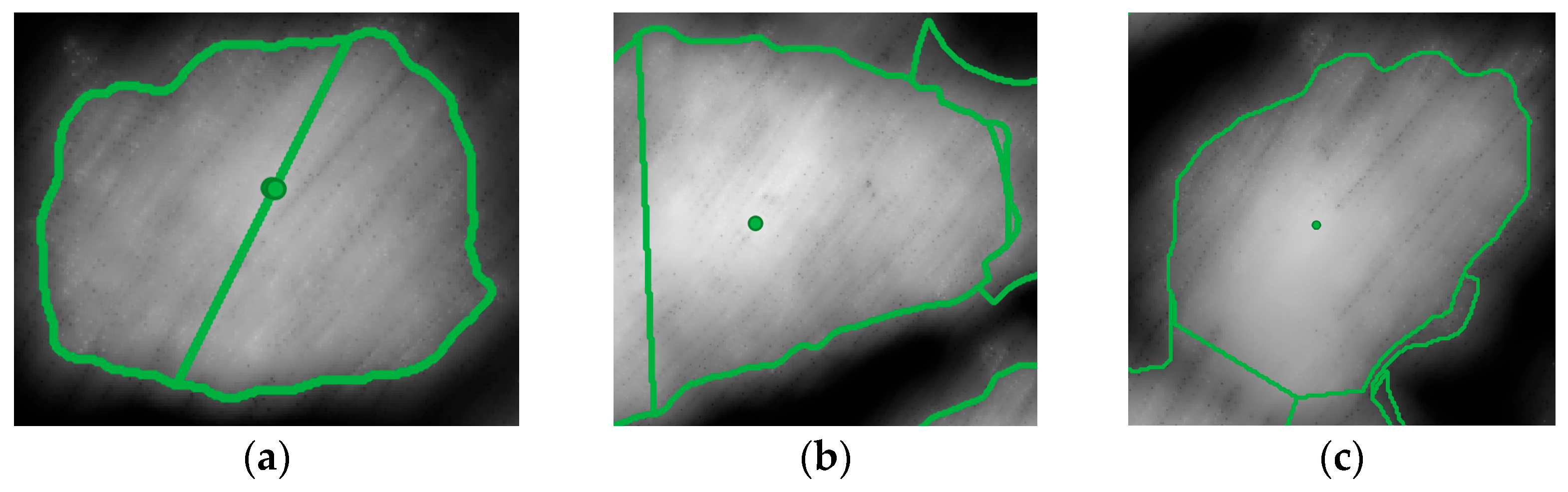
Additionally, it must be considered that the validation, although carried out by exploiting the knowledge of the position of the trees following the in situ measurement campaign, was mainly based on the user-defined visual interpretation of the point cloud and the CHM. This can be affected by discrepancies due to the subjectivity that affects the visual evaluations. Another aspect not to be overlooked is the difficulty in correctly delineating, both automatically and manually, the crown of trees when they are close to each other and the branches intersect each other.

As mentioned, the multitemporal matching procedure between the same trees acquired at different time instants is consistent and unique. As pointed out by [18], the comparison of forest elements through the use of an instrument that performs irregular sampling of points is complex; nevertheless, after having estimated the position of the tree as a function of the treetop, it is possible to carry out multitemporal analysis based on a unique tree parameter. The positive aspect is that it is possible to estimate the position of the treetops using data acquired from aerial laser scanners (by drones or helicopters). Clearly, the success of the procedure of identifying the same tree in multitemporal acquisitions strictly depends on the reliability of the segmentation procedure itself.

This is a challenging objective regarding the automatic estimation of tree parameters through remote sensing technologies [34]. If in more regular environments, as in the case of agricultural fields investigated in [35], good results are obtained even with a lower average density of points, the same is not valid for denser and more irregular areas. In particular, the density of the point cloud is considerably reduced in the description of the stem and of the lower branches, making it more difficult to estimate the DBH directly. The estimates, therefore, were made indirectly, using allometric equations [4,10] that made use of more easily estimated tree parameters (H and CD). However, errors in the estimation of forest variables can lead to a systematic error in estimating the parameters. In the proposed case study, the use of the proposed formulas highlighted a systematic underestimation of the DBH and the AGB. The reasons can be sought not only in the estimation of the variables, but also in the applicability of the allometric equations to predict the AGB and the DBH of any tree without making different considerations depending on the tree species.

Finally, with the aboveground biomass estimates, an assessment of the biomass lost in the area under examination due to the storm was carried out. The AGB estimate with Equation (5) was slightly worse than that obtained with Equation (2). This may be caused by the fact that the variable considered in Equation (5) (the DBH) is in turn estimated through Equation (1), which, as highlighted above, is affected in turn by underestimation, as seen previously. Finally, as seen in the DBH estimate, also in the case of the AGB, the best estimates were obtained by considering the scenario with the parameters automatically estimated. Only in the case of the 2014 scenario did manual segmentation seem to be more effective than that performed automatically, thanks to which the RMSE decreased by about 150 kg.

The results highlight the severity of the event, which destroyed about half of the biomass present; depending on the formula considered, it was estimated that the ice storm destroyed between 42% and 45% of the woody biomass, of which about 15–30% was irreversible.

5. Conclusions

In this study, we proposed an automated procedure to predict tree parameters on the single-tree-level using allometric equations that relate the DBH and the AGB to the tree height and the crown diameters. Additionally, we introduced the concept of multitemporal variability, comparing the parameters of the same tree over time; in this way, it is possible to study the evolution of forests at the level of a single tree and quantify the damage caused by a catastrophic natural event. The results are promising and emphasize the algorithm’s validity; however, this study should be considered as the first step in a broader analysis. First, this approach was tested on a relatively small area of interest; further areas with ground truth data will be considered to obtain results that can be considered more statistically robust. It is also necessary to evaluate the method’s accuracy under different forest conditions such as various tree species and forest densities, which can considerably influence the proposed method’s performance. Subsequently, further tests on treetop detection algorithms should be implemented. From the forest management point of view, the proposed approach can be very supportive, allowing for the acquisition of information on large areas in a reasonable amount of time. Moreover, implementing the latest LiDAR technologies on drones would increase the point density and the overall accuracy in smaller areas. Laser scanners equipped on helicopters can still be used to manage more extensive areas with reasonable accuracy, providing a greater quantity of information than other processing (e.g., photogrammetric analysis), thanks to the multiple returns of laser pulses. Moreover, the cost of collecting airborne LiDAR data is justified by the fact that in this way, it is possible to consider areas that are difficult to reach, and the safety of the operators is guaranteed.

Furthermore, among the future objectives, it would be important to be able to quantify the carbon stored within the aboveground biomass; in this way, it would be possible to also quantify the damage caused by a natural hazard from the perspective that the felled trees represent a loss of the capacity of the forest to stock carbon dioxide.

References

1. FAO. Global Forest Resources Assessment 2020; FAO: Rome, Italy, 2020. [Google Scholar] [CrossRef]
2. Coops, N.C.; Tompalski, P.; Goodbody, T.R.; Queinnec, M.; Luther, J.E.; Bolton, D.K.; White, J.C.; Wulder, M.A.; van Lier, O.R.; Hermosilla, T. Modelling lidar-derived estimates of forest attributes over space and time: A review of approaches and future trends. Remote Sens. Environ. 2021, 260, 112477. [Google Scholar] [CrossRef]
3. Latella, M.; Bertagni, M.B.; Vezza, P.; Camporeale, C. An Integrated Methodology to Study Riparian Vegetation Dynamics: From Field Data to Impact Modeling. J. Adv. Model. Earth Syst. 2020, 12, e2020MS002094. [Google Scholar] [CrossRef] [PubMed]
4. Jucker, T.; Caspersen, J.; Chave, J.; Antin, C.; Barbier, N.; Bongers, F.; Dalponte, M.; van Ewijk, K.Y.; Forrester, D.I.; Haeni, M.; et al. Allometric equations for integrating remote sensing imagery into forest monitoring programmes. Glob. Chang. Biol. 2017, 23, 177–190. [Google Scholar] [CrossRef]
5. Dalponte, M.; Frizzera, L.; Ørka, H.O.; Gobakken, T.; Næsset, E.; Gianelle, D. Predicting stem diameters and aboveground biomass of individual trees using remote sensing data. Ecol. Indic. 2018, 85, 367–376. [Google Scholar] [CrossRef]
6. Xu, D.; Wang, H.; Xu, W.; Luan, Z.; Xu, X. LiDAR Applications to Estimate Forest Biomass at Individual Tree Scale: Opportunities, Challenges and Future Perspectives. Forests 2021, 12, 550. [Google Scholar] [CrossRef]
7. Wulder, M.A.; White, J.C.; Nelson, R.F.; Næsset, E.; Ørka, H.O.; Coops, N.C.; Hilker, T.; Bater, C.W.; Gobakken, T. Lidar Sampling for Large-Area Forest Characterization: A Review. Remote Sens. Environ. 2012, 121, 196–209. [Google Scholar] [CrossRef]
8. Gleason, C.J.; Im, J. Forest biomass estimation from airborne LiDAR data using machine learning approaches. Remote Sens. Environ. 2012, 125, 80–91. [Google Scholar] [CrossRef]
9. Hickey, S.M.; Callow, N.J.; Phinn, S.; Lovelock, C.E.; Duarte, C.M. Spatial complexities in aboveground carbon stocks of a semi-arid mangrove community: A remote sensing height-biomass-carbon approach. Estuar. Coast. Shelf Sci. 2018, 200, 194–201. [Google Scholar] [CrossRef]
10. Chave, J.; Andalo, C.; Brown, S.; Cairns, M.A.; Chambers, J.Q.; Eamus, D.; Fölster, H.; Fromard, F.; Higuchi, N.; Kira, T.; et al. Tree allometry and improved estimation of carbon stocks and balance in tropical forests. Oecologia 2005, 145, 87–99. [Google Scholar] [CrossRef]
11. Salum, R.B.; Souza-Filho, P.W.M.; Simard, M.; Silva, C.A.; Fernandes, M.E.B.; Cougo, M.F.; Do Nascimento, W.; Rogers, K. Improving mangrove above-ground biomass estimates using LiDAR. Estuar. Coast. Shelf Sci. 2020, 236, 106585. [Google Scholar] [CrossRef]
12. Kankare, V.; Vauhkonen, J.; Holopainen, M.; Vastaranta, M.; Hyyppä, J.; Hyyppä, H.; Alho, P. Sparse Density, Leaf-Off Airborne Laser Scanning Data in Aboveground Biomass Component Prediction. Forests 2015, 6, 1839–1857. [Google Scholar] [CrossRef]
13. Torre-Tojal, L.; Bastarrika, A.; Boyano, A.; Lopez-Guede, J.M.; Graña, M. Above-ground biomass estimation from LiDAR data using random forest algorithms. J. Comput. Sci. 2022, 58, 101517. [Google Scholar] [CrossRef]
14. Dalponte, M.; Coomes, D.A. Tree-centric mapping of forest carbon density from airborne laser scanning and hyperspectral data. Methods Ecol. Evol. 2016, 7, 1236–1245. [Google Scholar] [CrossRef] [PubMed]
15. Xiao, W.; Xu, S.; Elberink, S.O.; Vosselman, G. Individual Tree Crown Modeling and Change Detection from Airborne Lidar Data. IEEE J. Sel. Top. Appl. Earth Obs. Remote Sens. 2016, 9, 3467–3477. [Google Scholar] [CrossRef]
16. Chen, W.; Hu, X.; Chen, W.; Hong, Y.; Yang, M. Airborne LiDAR Remote Sensing for Individual Tree Forest Inventory Using Trunk Detection-Aided Mean Shift Clustering Techniques. Remote Sens. 2018, 10, 1078. [Google Scholar] [CrossRef]
17. Di Pietra, V.; Grasso, N.; Piras, M.; Dabove, P. Characterization of a Mobile Mapping System for Seamless Navigation. Int. Arch. Photogramm. Remote Sens. Spat. Inf. Sci. 2020, XLIII-B1-2020, 227–234. [Google Scholar] [CrossRef]
18. Marinelli, D.; Paris, C.; Bruzzone, L. A Novel Approach to 3-D Change Detection in Multitemporal LiDAR Data Acquired in Forest Areas. IEEE Trans. Geosci. Remote Sens. 2018, 56, 3030–3046. [Google Scholar] [CrossRef]
19. Duncanson, L.; Dubayah, R. Monitoring individual tree-based change with airborne lidar. Ecol. Evol. 2018, 8, 5079–5089. [Google Scholar] [CrossRef]
20. Mograbi, P.J.; Erasmus, B.; Witkowski, E.; Asner, G.P.; Wessels, K.J.; Mathieu, R.; Knapp, D.E.; Martin, R.E.; Main, R. Biomass Increases Go under Cover: Woody Vegetation Dynamics in South African Rangelands. PLoS ONE 2015, 10, e0127093. [Google Scholar] [CrossRef]
21. Ali-Sisto, D.; Packalen, P. Comparison of 3D Point Clouds from Aerial Stereo Images and Lidar for Forest Change Detection. Int. Arch. Photogramm. Remote Sens. Spat. Inf. Sci. 2017, XLII-3/W3, 1–5. [Google Scholar] [CrossRef]
22. Waser, L.; Baltsavias, E.; Ecker, K.; Eisenbeiss, H.; Feldmeyer-Christe, E.; Ginzler, C.; Küchler, M.; Zhang, L. Assessing changes of forest area and shrub encroachment in a mire ecosystem using digital surface models and CIR aerial images. Remote Sens. Environ. 2008, 112, 1956–1968. [Google Scholar] [CrossRef]
23. Qin, R.; Tian, J.; Reinartz, P. 3D change detection—Approaches and applications. ISPRS J. Photogramm. Remote Sens. 2016, 122, 41–56. [Google Scholar] [CrossRef]
24. Nagel, T.A.; Firm, D.; Rozenbergar, D.; Kobal, M. Patterns and drivers of ice storm damage in temperate forests of Central Europe. Forstwiss. Centralblatt 2016, 135, 519–530. [Google Scholar] [CrossRef]
25. Zhang, W.; Qi, J.; Wan, P.; Wang, H.; Xie, D.; Wang, X.; Yan, G. An Easy-to-Use Airborne LiDAR Data Filtering Method Based on Cloth Simulation. Remote Sens. 2016, 8, 501. [Google Scholar] [CrossRef]
26. Lindsay, J. Whitebox GAT: A case study in geomorphometric analysis. Comput. Geosci. 2016, 95, 75–84. [Google Scholar] [CrossRef]
27. Zörner, J.; Dymond, J.; Shepherd, J.; Jolly, B. PyCrown—Fast Raster-Based Individual Tree Segmentation for LiDAR Data; Landcare Research NZ Ltd.: Lincoln, New Zealand, 2018. [Google Scholar] [CrossRef]
28. Zörner, J.; Dymond, J.; Shepherd, J.; Wiser, S.; Jolly, B. LiDAR-Based Regional Inventory of Tall Trees—Wellington, New Zealand. Forests 2018, 9, 702. [Google Scholar] [CrossRef]
29. Chave, J.; Réjou-Méchain, M.; Búrquez, A.; Chidumayo, E.; Colgan, M.S.; Delitti, W.B.; Duque, A.; Eid, T.; Fearnside, P.M.; Goodman, R.C.; et al. Improved allometric models to estimate the aboveground biomass of tropical trees. Glob. Chang. Biol. 2014, 20, 3177–3190. [Google Scholar] [CrossRef]
30. Zanne, A.E.; Lopez-Gonzalez, G.; Coomes, D.A.; Ilic, J.; Jansen, S.; Lewis, S.L.; Miller, R.B.; Swenson, N.G.; Wiemann, M.C.; Chave, J. Data from: Towards a Worldwide Wood Economics Spectrum; Dryad, Dataset: Oxford, UK, 2009; p. 2047488. [Google Scholar] [CrossRef]
31. Belcore, E.; Wawrzaszek, A.; Wozniak, E.; Grasso, N.; Piras, M. Individual Tree Detection from UAV Imagery Using Hölder Exponent. Remote Sens. 2020, 12, 2407. [Google Scholar] [CrossRef]
32. Ma, K.; Chen, Z.; Fu, L.; Tian, W.; Jiang, F.; Yi, J.; Du, Z.; Sun, H. Performance and Sensitivity of Individual Tree Segmentation Methods for UAV-LiDAR in Multiple Forest Types. Remote Sens. 2022, 14, 298. [Google Scholar] [CrossRef]
33. Qiu, L.; Jing, L.; Hu, B.; Li, H.; Tang, Y. A New Individual Tree Crown Delineation Method for High Resolution Multispectral Imagery. Remote. Sens. 2020, 12, 585. [Google Scholar] [CrossRef]
34. Weiser, H.; Schäfer, J.; Winiwarter, L.; Krašovec, N.; Fassnacht, F.E.; Höfle, B. Individual tree point clouds and tree measurements from multi-platform laser scanning in German forests. Biogeosci. Biodivers. 2022, preprint. [Google Scholar] [CrossRef]
35. Hadas, E.; Borkowski, A.; Estornell, J.; Tymkow, P. Automatic estimation of olive tree dendrometric parameters based on airborne laser scanning data using alpha-shape and principal component analysis. GISci. Remote Sens. 2017, 54, 898–917, Erratum in GISci. Remote Sens. 2017, 55, iii. [Google Scholar] [CrossRef]
Figure 1. The study area location (Dinaric Mountains, Southwest Slovenia). The red box defines the area covered by laser scans. EPSG: 3912.
Remotesensing 14 04666 g001
Figure 2. The workflow of the proposed method for the automatic detection of individual trees and the tree parameter estimation in multiple-time acquisitions.
Remotesensing 14 04666 g002
Figure 3. Example of the segmentation outcomes. (a) Over segmentation; (b) under segmentation; (c) correct segmentation. The layer shown is the CHM in grey scale.
Remotesensing 14 04666 g003
Figure 4. Segmentation and matching outputs. (a) Single-tree segmentation of the point cloud acquired in November 2013. (b) Crown shape and position of the trees in November 2013. (c) Single-tree segmentation of the point cloud acquired in April 2014. (d) Crown shape and position of the trees in April 2014. (e) Matched point cloud acquired in November 2013. (f) Matched point cloud acquired in April 2014. Trees with a multitemporal match plotted in colors; trees without a multitemporal match are plotted in dark blue. The ground points were not plotted to ease the visualization of the point clouds. EPSG: 3912.
Remotesensing 14 04666 g004
Figure 5. The error propagation of (a) Equation (1), (b) Equation (2), and (c) Equation (5) evaluated in percentage terms. (a,b) Error propagation with an error bias in the estimated crown diameter. (c) Error propagation with an error bias in the estimated DBH.
Remotesensing 14 04666 g005
Figure 6. The scatter plot of the DBH. Ground truth on the x-axis. (a) Scenario 1 estimates on the y-axis. (b) Scenario 2 estimates on the y-axis.
Remotesensing 14 04666 g006