Article

Proportional Similarity-Based Openmax Classifier for Open Set Recognition in SAR Images

1
National Laboratory of Radar and Surveillance Systems (RaSS), National Inter-University Consortium for Telecommunication (CNIT), 56124 Pisa, Italy
2
Department of Information Engineering, University of Pisa, 56126 Pisa, Italy
*
Author to whom correspondence should be addressed.
Remote Sens. 2022, 14(18), 4665; https://doi.org/10.3390/rs14184665
Submission received: 16 August 2022 / Revised: 10 September 2022 / Accepted: 15 September 2022 / Published: 19 September 2022
(This article belongs to the Special Issue SAR-Based Signal Processing and Target Recognition)

Abstract

:
Most of the existing Non-Cooperative Target Recognition (NCTR) systems follow the “closed world” assumption, i.e., they only work with what was previously observed. Nevertheless, the real world is relatively “open” in the sense that the knowledge of the environment is incomplete. Therefore, unknown targets can feed the recognition system at any time while it is operational. Addressing this issue, the Openmax classifier has been recently proposed in the optical domain to make convolutional neural networks (CNN) able to reject unknown targets. There are some fundamental limitations in the Openmax classifier that can end up with two potential errors: (1) rejecting a known target and (2) classifying an unknown target. In this paper, we propose a new classifier to increase the robustness and accuracy. The proposed classifier, which is inspired by the limitations of the Openmax classifier, is based on proportional similarity between the test image and different training classes. We evaluate our method by radar images of man-made targets from the Moving and Stationary Target Acquisition and Recognition (MSTAR) dataset. Moreover, a more in-depth discussion on the Openmax hyper-parameters and a detailed description of the Openmax functioning are given.

Graphical Abstract

1. Introduction

Radar imaging has been largely investigated in the literature as a means of equipping a radar system with automatic target recognition (ATR) capability. Many papers have demonstrated that radar systems can not only provide kinematic information (position, speed, and course) of land, sea, and air targets during day and night in all weather conditions but can also provide electromagnetic images of the targets, which can be used for recognition purposes [1,2,3,4,5,6]. Many algorithms have been proposed in the past decades showing that radar images of moving targets can be used for NCTR purposes. Few-shot target classification algorithms in Synthetic Aperture Radar (SAR) have also been intensively studied in recent years [7,8]. The most promising algorithms are based on a training step and, therefore, require a set of data from known targets. Furthermore, many recent papers have shown that deep networks (DN) can provide high-performance recognition [4,5,6]. However, they require a priori knowledge about the targets. While it is possible to train such a system with terabytes of data, it is impossible to anticipate and train with all possible inputs that a classifier may encounter in a real-world scenario. The real data are inherently dynamic and hence difficult to predict. So far, most state-of-the-art NCTR systems have followed a “closed world” assumption, meaning that the system model is complete and the system can reason using what was observed previously [9,10,11,12,13,14]. However, this assumption is not realistic and leads to fragile systems that can fail at inference time [15]. The real world contains an open set of targets, and any system knowledge (as also our knowledge) is incomplete. This problem has been more thoroughly investigated in the computer vision field rather than the radar field. Some studies tackled the above-mentioned problem, which is known as open set recognition (OSR), by applying a threshold to the Softmax function [16,17]. Softmax, which is a typical classifier in convolutional neural networks (CNN), maps the activation vector into a probability domain. The activation vector refers to the output of the last fully connected (FC) layer [18]. Note that imposing a threshold on Softmax’s outputs is not a practical solution, since CNNs may generate incorrect large scores in the case of open set inputs.
To overcome this issue, the Openmax algorithm [18] has been recently proposed in the optical domain that drops the restriction for the output scores to sum to one. Therefore, it allows the model to recognize the input as an unknown image without necessarily requiring any threshold. Using a conditional generative adversarial network (GAN) to synthesize mixtures of unknowns, Ge et al. [19] proposed the Generative Openmax (G-Openmax) algorithm, which enables a classifier to locate the decision margin according to the knowledge of known classes and the generated unknown samples. However, such unknowns are limited to the subspace of the known classes [20]. Zheng et al. [21] proposed a model based on an autoencoder and an auxiliary classifier to generate pseudo samples. They then used the generated samples to improve out-of-distribution detection performance in natural language understanding by optimizing the entropy regularization term in the training stage. It should be noted that adversarial images cannot fully represent the open set environment. Lee et al. [22] proposed a method for detecting either out-of-distribution or adversarial samples by measuring the Mahalanobis distance between the test sample and the closest class-conditional Gaussian distribution. Inkawhich et al. [23] showed that a large, unlabeled, and unrelated SAR dataset can be used to improve the out-of-distribution detection in SAR-ATR applications. Note that ATR using SAR images is more challenging than optical images since SAR images have lower signal-to-noise ratios (SNR) and lower spatial resolution than optical images. In this regard, in our previous studies [24,25], we have first investigated the applicability of the Openmax classifier for SAR images and then analyzed the possibility of having class-wise hyper-parameter (tail size) and distribution type to optimize the tail-fitting procedure in the Openmax approach. It is worth noting that the standard Openmax approach takes only one tail size value, which should be set heuristically in the calibration phase, and assumes only one distribution type (Weibull), i.e., the same tail size and the same distribution type for all the classes. However, we noticed that each class has a distinctive distance distribution, and if we change the algorithm and carefully set the tail size and the distribution type in each class separately, the overall accuracy will improve significantly. This implies that there exists an imbalance between the classes. However, such an optimization problem (on the hyper-parameters) requires a priori knowledge about the classes that is hard to be achieved in a real-world SAR scenario where a target observed by a slightly different aspect angle may change significantly.
In this paper, with the aim of improving the overall accuracy and robustness of OSR in SAR images, we base our proposed method on the limitations of the Openmax algorithm. The reason why we choose the Openmax classifier and not any of the adversarial-based solutions for this application is that Openmax exploits the statistical information of the training dataset to recognize possible unknown inputs, and it is not based on training with some counterfactual image that cannot technically represent all possible open set inputs. There are two types of errors that the Openmax classifier may encounter: some closed set images may mistakenly be recognized as unknown and some open set images may mistakenly be classified as one of the closed set classes. We have studied different aspects of the Openmax classifier when applied to the target recognition in SAR images and identified the following items as the main sources of two aforementioned errors: feature extraction, tail-fitting, and activation vector modification. We then propose a substitute for the tail-fitting procedure that relies on the interrelations between the test image and different training classes. It is worth noting that the standard Openmax modifies each element of the activation vector based on the similarity between the test image and only the corresponding class of the training set and not other training classes. However, our new method considers also the relationship that exists among the training classes. In other words, the new method makes use of the similarity between the test image and the different training classes in proportion to the similarity between the training classes to modify the activation vector. Therefore, the proposed approach is hereafter called proportional similarity-based Openmax or simply PS-Openmax. In the end, we used the Moving and Stationary Target Acquisition and Recognition (MSTAR) dataset [26] for the experimental verification. The contributions of the paper are threefold:
  • A thorough examination of the Openmax classifier and a detailed discussion on the tail-fitting procedure in different OSR scenarios.
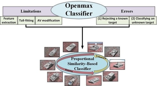
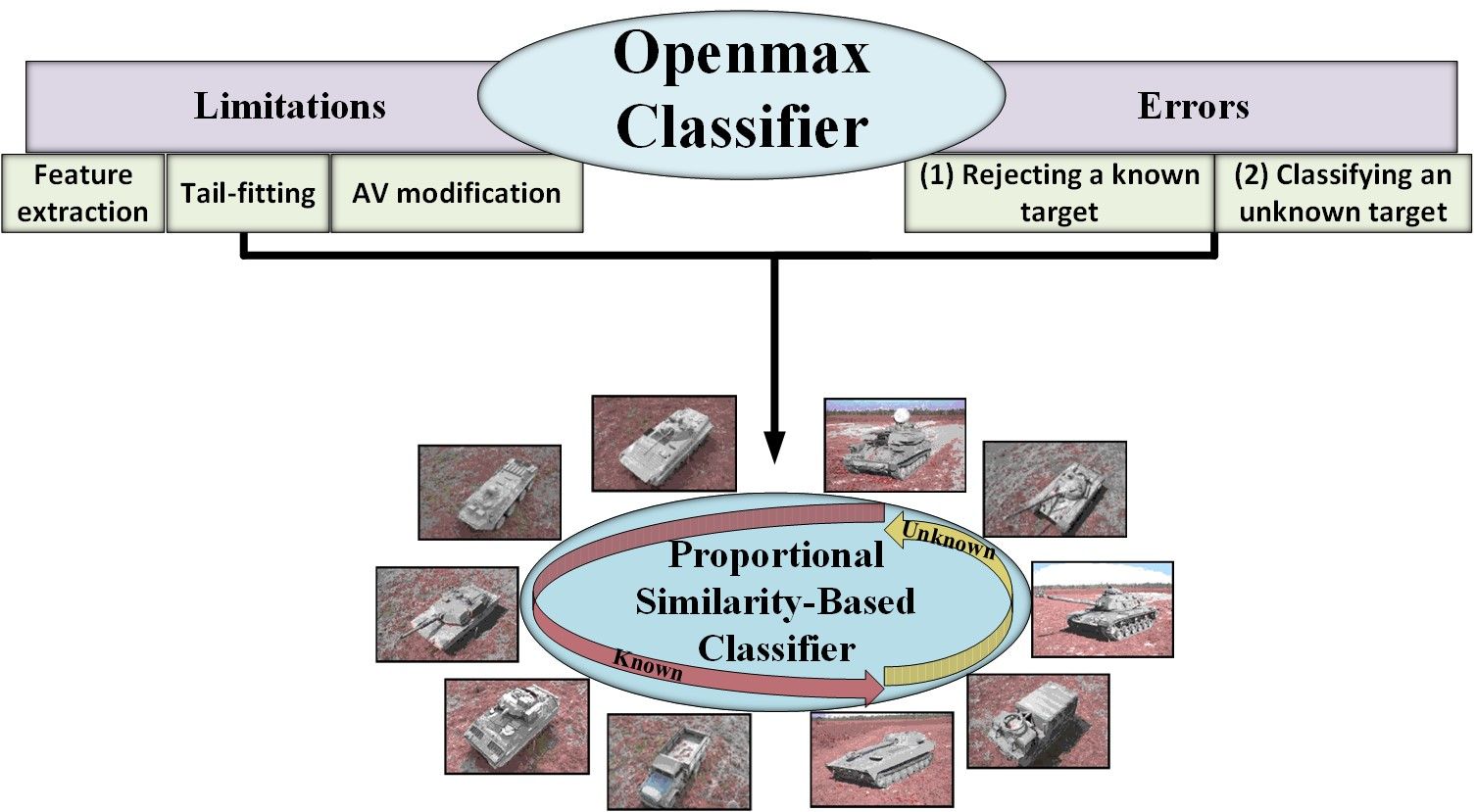
  • An analysis of the Openmax limitations and source of errors to effectively avoid the situations where either a known or an unknown target is always misclassified.
  • Proposing the proportional similarity-based approach, which makes use of the similarity between the test image and different training classes in proportion to the similarity between the training classes, to increase the robustness and the accuracy.
This paper is organized as follows. Section 2 presents the materials and methods. Section 3 shows the experimental results. Section 4 provides discussion and analysis of the methods. Section 5 concludes this paper.

2. Materials and Methods

In this section, the materials and methods required for the real data experiments are described. First, the Openmax approach is briefly introduced in Section 2.1. Subsequently, the proposed approach is comprehensively explained in Section 2.2. Finally, the experimental setup and materials are introduced in Section 2.3.

2.1. The Openmax Approach

In classification tasks, the Softmax layer is typically used at the end of the network to map the output of the last FC layer, namely “activation vector (AV)”, into scores that sum to one. Defining x as the input image and N as the number of closed-set classes, the Softmax score of the class c can be computed by its corresponding activation score AV c ( x ) , which is divided by a summation over all activation scores, as follows:
s s o f t c = e A V c ( x ) i = 1 N e A V i ( x )
Given the softmax scores for all the classes as s s o f t = [ s s o f t 1 , , s s o f t c , , s s o f t N ] , the easiest way to address the open set problem is to impose a certain threshold to m a x ( s s o f t ) . In other words, if none of s s o f t scores of the test image exceeds a certain threshold s t h , the test image will be recognized as an unknown.
if   m a x ( s s o f t ) > s t h c l a s s = a r g m a x ( s s o f t ) else c l a s s = u n k n o w n
Openmax [18], as an alternative to the Softmax threshold approach, modifies the definition of the Softmax function to include an unknown class. The Openmax procedure is composed of two phases: the model calibration and the calculation of the Openmax scores. The model calibration phase is described in Algorithm 1, and it takes two input types: (1) the outputs of the last FC layer of the network and (2) the scalar η , as a hyper-parameter for the ‘tail size’ in the calibration process. Note that only the correctly classified training images will be used again in the calibration phase. In fact, AV 1 t r a i n and AV N t r a i n in the input line denote the activation vectors of the images in the training classes 1 and N, respectively.
The Openmax classifier is employed for a pre-trained CNN where the last layer of the CNN is an FC layer with N neurons. It modifies the final output, i.e., AV, and generates a modified AV to have N + 1 elements where the last element represents the unknown class, and it then maps the modified AV to the probability domain. By a pre-trained CNN, we mean that the model should be first trained using the training dataset and then the statistical features of the training data, i.e., known targets, are extracted to design the classifier that is able to recognize unknown test data. Considering one of the training classes as an example and computing the mean activation vector (MAV) of this class, see line 2 of Algorithm 1, the Openmax fits a Weibull distribution to the tail of Euclidean distances between AVs and MAV of this class; see lines 3 and 4 of Algorithm 1. LibMR, which is a publicly available library (https://github.com/Vastlab/libMR (accessed on 15 August 2022)), provides the FitHigh function for the maximum likelihood estimation using the Weibull distribution.
More specifically, in line 3 of Algorithm 1, the Euclidean distance values among MAV and all AVs of each class are computed and sorted. Next at line 4, a Weibull distribution is fitted to the η largest distances. The outputs of Algorithm 1 are the Weibull model and MAV measured for each training class. The Weibull distribution is commonly used since it has been demonstrated to be the most suitable distribution for statistical meta-recognition [27,28]. Nonetheless, a deep analysis considering different types of distributions is also included in this work; see Section 3.4.
Algorithm 1 Model Calibration
     Input: AV 1 t r a i n , …, AV N t r a i n , η
     Output: (Weibull 1 t r a i n , MAV 1 t r a i n ), …, (Weibull N t r a i n , MAV N t r a i n )
1: for j = 1, 2, …, N do
2:    MAV j t r a i n = mean(AV j t r a i n )
3:    ED j t r a i n = sort(EuclideanDistance (AV j t r a i n , MAV j t r a i n ))
4:    Weibull j t r a i n = FitHigh (ED j t r a i n , η )
Considering a test image, the Openmax second phase is summarized in Algorithm 2.
Algorithm 2 Openmax scores calculation
     Input: (Weibull 1 t r a i n , MAV 1 t r a i n ), …, (Weibull N t r a i n , MAV N t r a i n ), AV of the test image, N α
     Output: Openmax scores
1: o r d = argsort(AV, “descending”)
2: for i = 1, …, N α  do
3:     j = o r d ( i )
4:     C D = EuclideanDistance( A V M A V j t r a i n )
5:     τ , κ , λ = Weibull j t r a i n
6:     w = 1 e C D τ λ κ
7:     α = ( N α i + 1 )/ N α
8:     m o d A V ( j ) = A V ( j ) ( 1 w × α )
9: u n k = j = 1 N ( A V ( j ) m o d A V ( j ) )
10: modAV (N + 1) = unk
11: for j = 1, 2, …, N + 1 do
12:     s o p e n j = e m o d A V ( j ) k = 1 N + 1 e m o d A V ( k )
13: s o p e n = [ s o p e n 1 , s o p e n 2 , , s o p e n N + 1 ]
In short, the Openmax subtracts a portion from each element of AV based on the similarity of the test image and the respective training class, sums the subtracted values, and forms a modified AV with one more element appended to its end to represent the unknown class. The algorithm takes three input types: (1) MAV and the Weibull model pair for each training class from Algorithm 1 together with (2) the activation vector of the test image, i.e., AV, and (3) the scalar N α as another hyper-parameter. By computing the Openmax scores, i.e., s o p e n = [ s o p e n 1 , , s o p e n c , , s o p e n N + 1 ] , the corresponding index to the maximum value determines the class assigned to the test image. Note that only the top N α values of AV will be modified and the rest of the N N α elements of AV will be untouched. To select the changeable elements, AV is sorted at line 1 of Algorithm 2, and the corresponding indexes are used at line 3 to modify the jth element of AV. More in detail, Openmax calculates two factors, i.e., ‘ α ’ and ‘w’, to modify each element of AV. In order to calculate ‘w’ for the modification of the jth element of AV, Openmax first calculates the channel distance (CD) scalar value, see line 4 of Algorithm 2, based on the distance between AV and MAV of the class j. It then evaluates the value of Weibull cumulative distribution function (CDF) of the class j, from Algorithm 1, on the channel distance point; see lines 5 and 6 of Algorithm 2. The other factor for the modification of the jth element of AV is α ; see the rule at line 7 of Algorithm 2. For instance, if we assume N α = N = 8 , i.e., the scenario where we have eight known classes and we want to modify all eight elements of AV, then α = 1 , 0.875 , 0.75 , 0.625 , 0.5 , 0.375 , 0.25 , 0.125 will be generated iteratively. Afterward, as we have mentioned before, w together with α are used to modify the j t h element of the activation vector AV; see line 8 of Algorithm 2. Note that the new element of AV to represent the unknown class is made up of the subtracted values. In other words, the difference between the original activation vector AV and the modified activation vector m o d A V is summed up, see line 9 of Algorithm 2, and it is then appended to the modified activation vector m o d A V , at line 10, as the activation score of the unknown class. In the end, the m o d A V , i.e., the one with N + 1 elements, is mapped to the probability domain to generate the Openmax scores; see lines 12 and 13 of Algorithm 2.

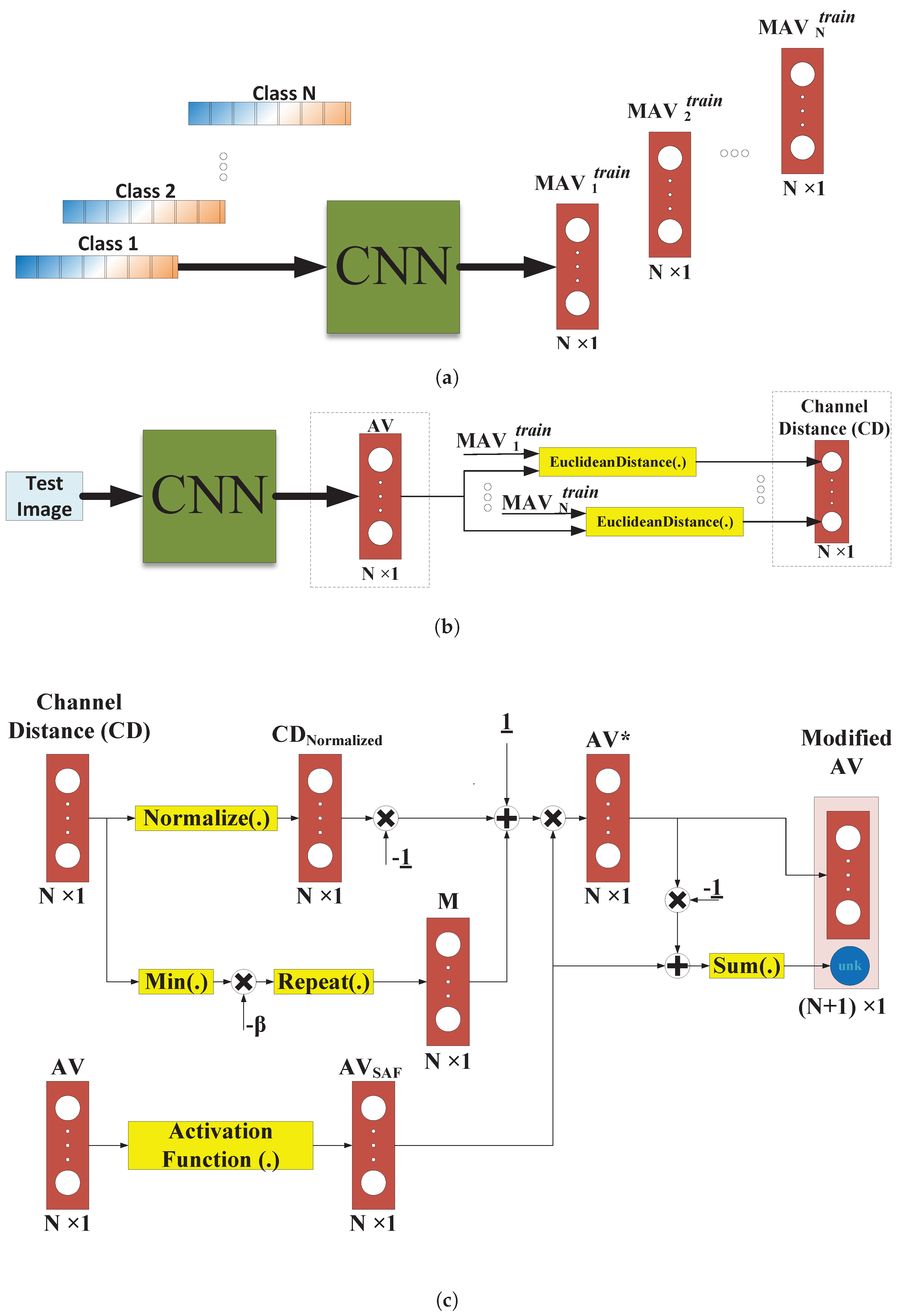
2.2. The Proposed Approach
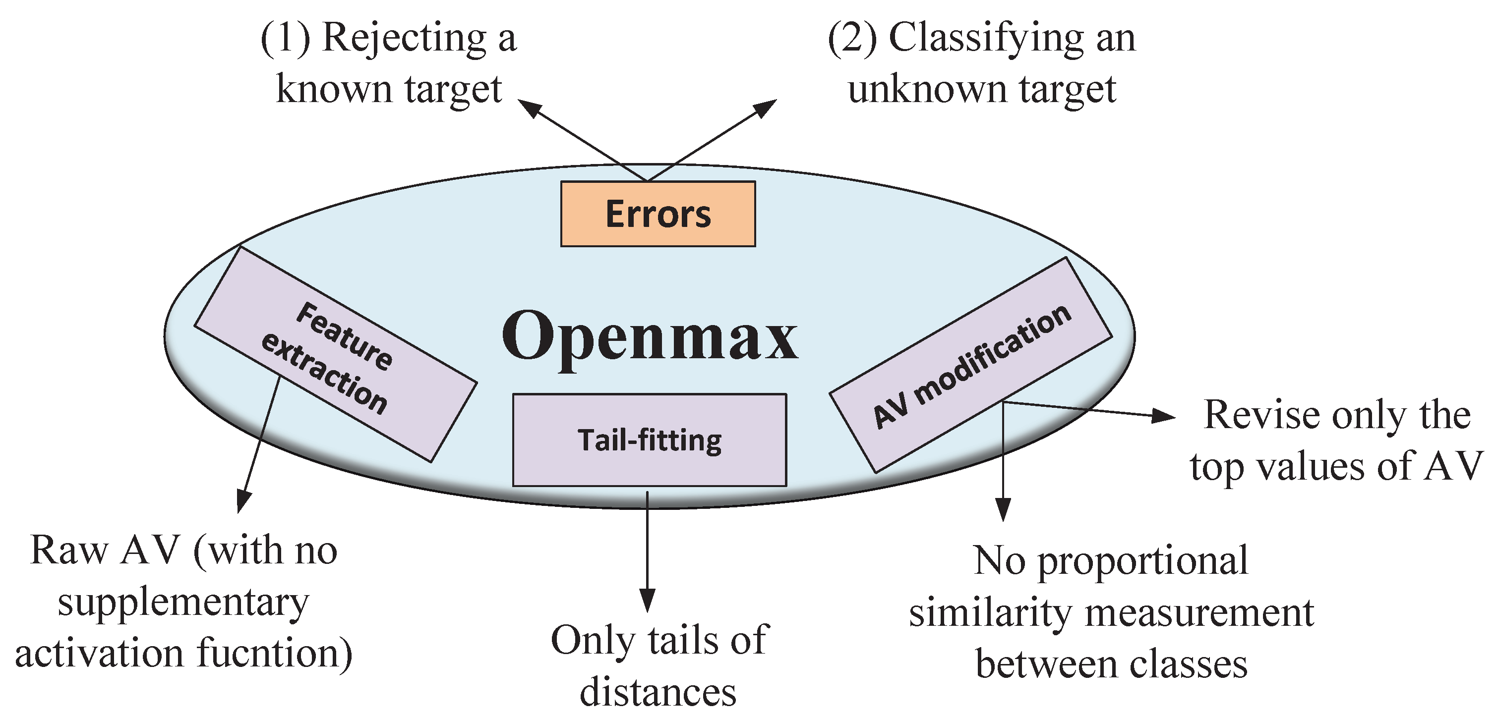
In this section, first, we highlight some of the inherent limitations of the Openmax classifier, and then, we propose our proportional similarity-based classifier, which obviates these limitations. As illustrated in Figure 1, there are two types of errors that Openmax may encounter: (1) recognizing a known input image as an unknown and (2) recognizing an unknown input image as a known class. The main source of these two errors should be searched in features extraction, tail-fitting, and AV modification:
  • Feature extraction:
    In the Openmax classifier, the raw outputs of the last FC layer are directly used for the scores calculations. However, in the new method, a supplementary activation function is used to map the AV into another domain that is more suitable for the OSR problem. It should be noted that the supplementary activation function will be only used during the inference and not in the training. In fact, only the Softmax activation function is applied to AV in the training phase.
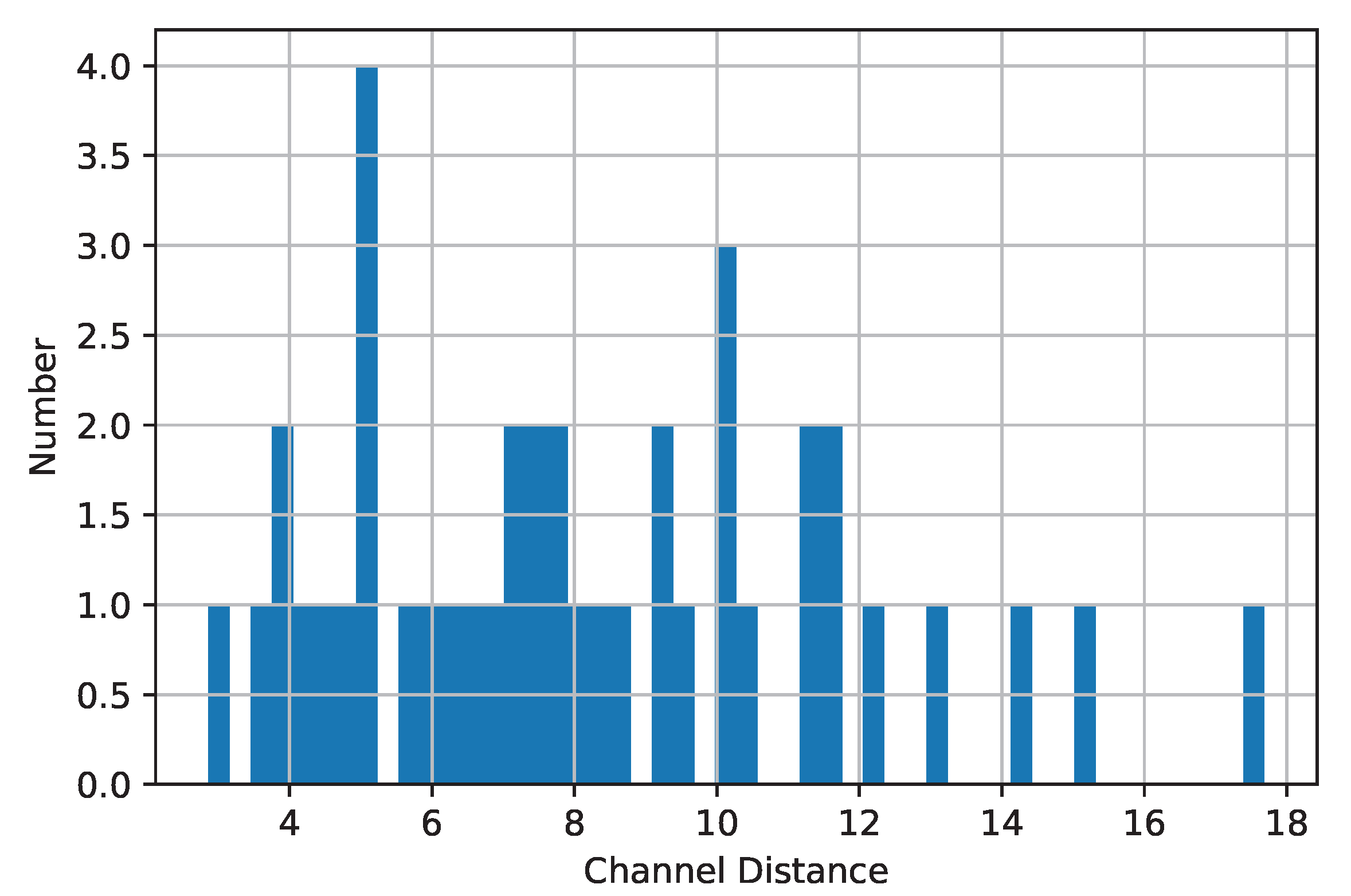
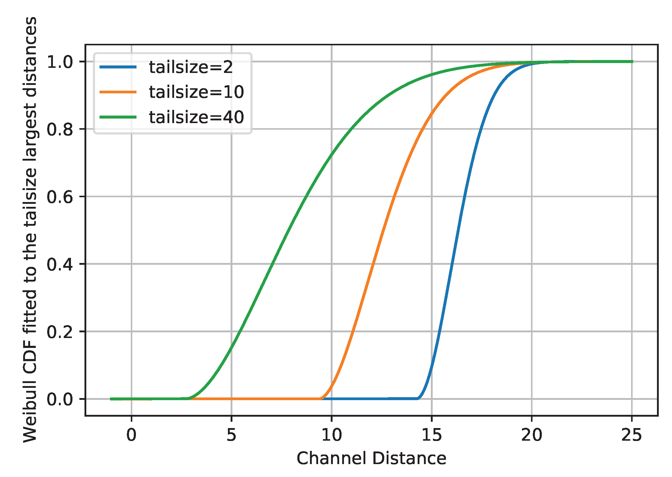
  • Tail-fitting procedure:
    The distance values and their distributions can contain useful information for the OSR solution. The most critical hyper-parameter of Openmax is η by which it analyzes only the tail of distance values. However, a more accurate OSR solution can be designed by exploiting full information of distance values.
  • Activation vector modification:
    (a)
    The choice of N α :
    It is worth mentioning that N α is another hyper-parameter in the original Openmax, and similar to η , it has to be carefully chosen beforehand. By modifying only the top N α values of AV, i.e., subtracting different portions from those elements, Openmax generates an extra class dedicated to the unknown inputs. In fact, Openmax takes N α < N to reduce the number of changeable neurons in AV, especially in the case of CNNs that generate some negative scores in their AV. Therefore, the aim of N α < N is to discard some of the negative values of AV, in other words, to exclude N N α smallest values of AV, in order to avoid the new element from having a possibly large negative value. This large negative value forces the classifier not to reject the unknown input image and ends up with the second error shown in Figure 1. Note that by discarding some of the negative values of AV using N α < N , the original Openmax lets the new element have the largest value in the case of an unknown input image. However, choosing N α < N in the original Openmax implies a priori knowledge. We will introduce our PS-based classifier that obviates this limitation and has an improved performance toward unknown images.
    (b)
    Class-independent subtraction:
    According to the CNN model and the input test image, it is also quite probable that the new element of AV ends up being a very large positive value and the first error shown in Figure 1, i.e., rejecting a known image, happens. This problem is likely to happen in CNNs that do not generate negative scores in their AV. Therefore, even by reducing the number of changeable neurons in AV, i.e., N α < N , it is still probable that the new element becomes the greatest one, and this forces the classifier to reject the known image. Note that in the original Openmax classifier, the subtraction in each element of AV is performed independently from the others, and the relationship between different classes is not studied. By exploiting this aspect, the PS-based classifier provides an improved accuracy toward the input images of the known classes.
Considering the aforementioned limitations, we propose our PS-based classifier, as an extension to Openmax, to improve its robustness and accuracy toward both known and unknown classes. Similar to the original Openmax classifier, the PS-based classifier will also be employed for the pre-trained CNN, and it modifies the AV from N elements to N + 1 elements. The distinctive feature of the proposed method is to consider the relationship between the test image and all the training classes when modifying each element of the AV. The overall framework of the proposed method is illustrated in Figure 2, and its pseudo-code is formulated in Algorithm 3.
The proposed method makes use of a supplementary activation function, takes advantage of all distance information rather than the tails, and provides a different perspective for modifying AV. The inputs of the proposed method, as shown in Algorithm 3, are the MAVs of known classes and the AV of the test image. MAVs, which are illustrated in Figure 2a, are calculated in the same way as in the original Openmax method.
Algorithm 3 PS-Openmax scores calculation
     Input: (MAV 1 t r a i n , …, MAV N t r a i n ), AV of the test image
     Output: PS-Openmax scores
1: for i = 1, …, N do
2:     C D i = EuclideanDistance ( A V M A V i t r a i n )
3: C D N o r m a l i z e d = C D i = 1 N C D i
4: M = β [ m i n ( C D ) , , m i n ( C D ) ] T
5: AV S A F = AV-min(AV)
6: AV =[1+M-CD N o r m a l i z e d ] AV S A F
7: u n k = j = 1 N ( A V S A F ( j ) A V ( j ) )
8: M o d i f i e d A V = [ A V , u n k ]
9: for j = 1, 2, …, N + 1 do
10:     s p s j = e M o d i f i e d A V ( j ) k = 1 N + 1 e M o d i f i e d A V ( k )
11: s p s = [ s p s 1 , s p s 2 , , s p s N + 1 ]
Considering the test image, we form the Channel Distance vector from all the classes at lines 1 and 2 of Algorithm 3. This part has been illustrated in Figure 2b where the Channel Distance vector and the AV of the test image are surrounded by dashed boxes to be used in Figure 2c. Note that in the original Openmax (see line 4 of Algorithm 2), channel distance is scalar and is only computed for the top N α elements of AV.
In line 3 of Algorithm 3, we calculate the normalized Channel Distance vector, i.e., C D N o r m a l i z e d , to evaluate the proportional relationship among its elements and to effectively avoid the situation that the absolute value of the last element of the AV is always too large. This aspect, i.e., the interrelation between different channel distance values, has not been studied in the original Openmax, and channel distance values were separately (independently) used to modify their corresponding elements of AV. Next, the minimum value of the Channel Distance vector is also taken into account as a parallel measure at line 4 of Algorithm 3. Note that m i n ( C D ) is repeated to form a N × 1 vector and β ( 0 , 1 ) as a hyper-parameter is used to balance between the two factors: minimum channel distance and the normalized Channel Distance vector.
Typical activation functions, such as Sigmoid, Tanh, Softmax, ReLU, and its variants are employed in an element-wise way. We instead propose the supplementary activation function AV-min(AV) as a vector form activation function to make sure that none of the elements in AV is negative. This supplementary activation function is applied at line 5 of Algorithm 3 to generate AV S A F . This supplementary activation function has been chosen through an extensive series of experiments performed on different activation functions.
In the proposed method, we modify the AV S A F in an element-wise manner by using two factors: M, i.e., the minimum channel distance, and C D N o r m a l i z e d , i.e., the normalized Channel Distance vector, using the Hadamard product (∘); see line 6 of Algorithm 3. By calculating the sum of the differences between AV S A F and AV , a new element (shown in blue in Figure 2c) is formed; see line 7 of Algorithm 3. Similar to the original Openmax, the new element is appended to the end of Modified AV, see line 8 of Algorithm 3, and the Modified AV is mapped to the probability domain to generate PS-Openmax scores; see lines 9–11 of Algorithm 3.
In summary, the tail-fitting procedure is substituted with a measure of proportional similarity in the PS-Openmax approach, and using the relationship among the Channel Distance values prevents the new element from having always a too large negative value or a too large positive value. Note that there is neither a need to limit the number of changeable neurons in AV, i.e., choosing N α , nor to calibrate tail size.

2.3. Experimental Setup and Materials

In this part, the experimental setup is defined. First, the CNN structure is described in Section 2.3.1. Afterward, the dataset is introduced in Section 2.3.2, and finally, the performance indexes are defined in Section 2.3.3.

2.3.1. CNN Structure

The CNN structure used to test the proposed approach is shown in Table 1.
It consists of three convolutional layers (Conv1, Conv2, and Conv3), two pooling layers (MaxPooling1 and MaxPooling2), and two FC layers (FC1 and FC2). All the convolution layers are followed by ReLU functions. After a convolution layer, a pooling layer is introduced to reduce the dimensions of convolution layer outputs. The last FC layer is followed by an 8-class Softmax classifier. The Softmax classification module maps the output of the last FC layer to the probability domain as mentioned in (1). The kernel size of the first two convolutional layers is 3 × 3 , whereas that of the last convolutional layer is 5 × 5 and all pooling layers have 2 × 2 kernels. Moreover, the stride is set to zero, and zero-padding on borders is applied to avoid the shrinking of feature maps after the convolutional layers. The CNN is implemented by Keras, where the cross-entropy loss function is minimized via the Adam optimization algorithm with a learning rate equal to 0.0001 and the batch size of 8.

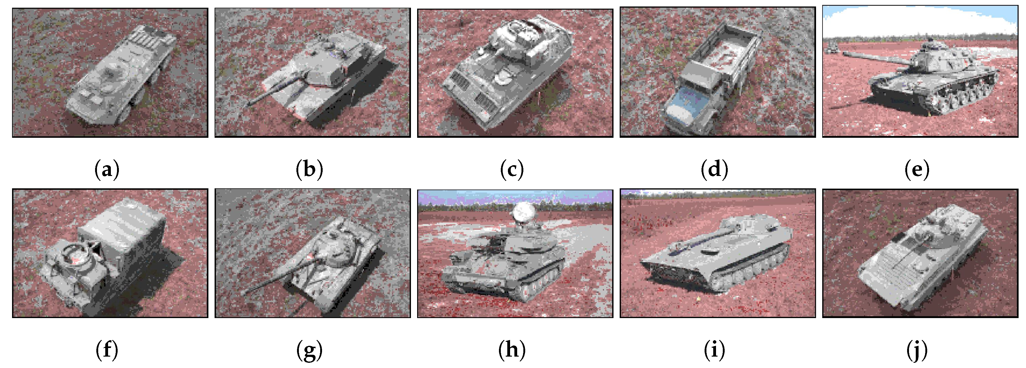
2.3.2. Dataset Description

We perform our real data experiments using the well-known MSTAR dataset [26]. MSTAR has been widely used by so many scholars for the training and evaluation of SAR-ATR applications, specifically for deep learning methods [5,28,29,30,31,32]. To be more specific, a part of the MSTAR dataset, which has also been chosen by [29], is used for training and test. The dataset consists of the real SAR images of ten different ground targets of air defense unit (ZSU-23-4), armored personnel carrier (BMP-2, BTR-70), tank (T-72, M-60, M-1, M-2), rocket launcher (2S1), military cargo carrier (M548) and light utility truck (M35). They have been collected by an X-band SAR sensor (9.6 GHz) with 0.3 m by 0.3 m resolution in spotlight mode and full 360 aspect angles coverage.
Each chip has an approximate size of 128 × 128 pixels, although we reshape all the images to the size of 64 by 64 pixels. Under the standard operating conditions (SOC), two depression angles of 17 and 15 , as a matter of routine, are used separately for the train and test sets, respectively [33]. The electro-optical images corresponding to the MSTAR dataset used in this paper are shown in Figure 3.
Let us assume that there are eight known classes (0–7) and two unknown classes (8, 9). In fact, we want to train a CNN with only eight classes (0–7) and test it with all ten classes (0–9) and see if the model is not only able to correctly classify images of the known classes (0–7) but is also able to reject images that belong to open set or unknown classes (8–9). Based on the concept of “Openness”, which has been introduced and formulated by Scheirer et al. [34], the complexity of an open set recognition problem can be expressed by the number of target classes to be identified, the number of classes used in training, and the number of classes used in testing as
O p e n n e s s = 1 2 × | t r a i n i n g c l a s s e s | | t e s t i n g c l a s s e s | + | t a r g e t c l a s s e s |
where | . | represents the number of classes in each respective set. Note that the problem is completely closed when the O p e n n e s s equals to zero whereas larger openness, i.e., close to one, corresponds to more open problems [20]. In our scenario, | t r a i n i n g c l a s s e s | = 8 and | t e s t i n g c l a s s e s | = | t a r g e t c l a s s e s | = 10; therefore, O p e n n e s s is equal to 0.1. Note that in an extreme case such as training with only one class and testing with ten classes of our dataset, O p e n n e s s reaches 0.68. It is also possible to add more unknown classes from the optical domain, such as the one we will analyze later in Section 3.2; however, these scenarios do not constitute a challenge for the classifier. Moreover, there is a large discrepancy between SAR and optical images, and because of the high cost of SAR image acquisition, a large-scale annotated dataset for the network training is rare [35].

2.3.3. Performance Indexes

The classifier performance will be assessed in terms of both the confusion matrices and a number of performance indexes that are commonly used. The well-known confusion matrix is typically a square matrix C M R N × N that measures the classifier capability in processing the test dataset. Differently, in this case, the unknown class is included in the confusion matrix to measure the ability of the classifier to correctly recognize both known targets and unknown targets. In particular, there are two input unknown classes and one output unknown class. Therefore, in our scenario, C M R N + 2 × N + 1 , and the confusion matrices reported in Section 3 are rectangular and not square. Four different performance indexes based on our non-square C M can be defined: namely, the Precision, P r , the Recall, R e , the F1-score, F 1 , and the total Accuracy, A c , as follows:
P r [ k ] = C M [ k , k ] n = 1 N r C M [ n , k ]
R e [ k ] = C M [ k , k ] n = 1 N c C M [ k , n ]
F 1 [ k ] = 2 P r [ k ] R e [ k ] P r [ k ] + R e [ k ]
A c = C M [ N + 2 , N + 1 ] + n = 1 N + 1 C M [ n , n ] n = 1 N r i = 1 N c C M [ n , i ]
where N c = N + 1 and N r = N + 2 are the number of columns and rows of the confusion matrix, respectively. In addition, N = 8 is the number of known classes, and k = 1 , , N + 1 is the class index. P r is the ratio of correctly predicted positive observations to the total predicted ones. High values of P r mean a low false positive rate. R e is the ratio of correctly predicted positive observations to the all observations in the true class. It is also known as the sensitivity. It can be interpreted as a measure of the missed detection. F1 is a useful metric, which takes both P r and R e into account and can be defined as the harmonic mean of the P r and R e . The total A c is defined as the mean rate of correctly classified samples [36].

3. Results

This section shows the main results achieved by Softmax, Openmax, and PS-based Openmax classifiers applied to the dataset described in Section 2.3.2. More specifically, the Openmax calibration procedure is described in Section 3.1. Openmax provides calculations for three different input image: one known image from the class 0, one unknown image from the MSTAR dataset and one optical unknown image are summarized in Section 3.2. The classification results of Openmax and Softmax are deeply analyzed in Section 3.3. The discussions on the choice of the tail size and the CDF are reported in Section 3.4. In the end, the results of the proposed PS-based approach are analyzed in Section 3.5. The reason why the proposed PS-based approach has been analyzed separately is that it does not contain tail-fitting procedure, so it is out of the tail size analysis and the CDF type discussion.

3.1. Openmax Pre-Processing

The results shown in this section have been obtained by training the network shown in Table 1 using the image dataset shown in Table 2.
The trained network is evaluated by the training dataset to determine the corrected-classified image set, T t r a i n . In this scenario, all the training images are classified correctly, as expected. For each image of T t r a i n , the outputs of layers eight and nine, i.e., activation vector (AV), and the Softmax output, are taken into account. The matrix M R 8 × 8 is then computed as follows:
M = M A V 1 M A V i M A V 8
where i = 1 , 2 , , N , N = 8 is the number of known classes, and M A V i R 1 × 8 represents the mean vector of the AV vectors of the class i. The matrix M is computed by the training set, and it is illustrated in Table 3. Then, the Euclidean distance between the AV of each image and the MAV of its class (one row of M) is computed. As a result, each image in the training set has an associated Euclidean distance value. As explained previously, the η largest Euclidean distances in each class is then used to fit a Weibull distribution. In this part, the MAV and Weibull CDF of each class are considered as the outputs.

3.2. Openmax Preliminary Test

After performing all the above pre-processing steps, the test images will be processed. In order to measure the channel distance (CD) values, the Euclidean distance between the AV of the test image and each row of M is calculated. Based on the Weibull CDFs generated in the previous part and the CD values, w is subsequently calculated, as also specified in line 6 of Algorithm 2, to modify the AV of the test image. Considering that 0 w 1 , it is obvious that m o d A V can contain values equal to or smaller than those in AV and the differences are reserved for the unknown class. Note that the length of the m o d A V vector is N + 1 , such that i = 1 ( N + 1 ) m o d A V = i = 1 N A V , and the new element represents the activation score of the unknown class.
To make it more clear, the overall classification process of three different images is described in detail hereinafter. Let us consider a test image from the class 0. The classification results and their intermediate steps are reported in Table 4. The tail size has been set to 10 in this case. As can be seen at line 2 of Table 4, the C D value is minimum for the class 0. This shows that by having C D = 5.53, the AV of the test image is closer to the MAV of class 0 compared with other MAVs. As a consequence, w or the corresponding Weibull CDF evaluated on the C D is also minimum for class 0. Note that the Softmax classifier classifies this image correctly. Based on AV, α values are calculated at line 5 of Table 4 as described mathematically at line 7 of Algorithm 2. Then, the AV vector is decomposed into the m o d A V and ( A V m o d A V ) . This means that for each class, a certain amount of AV is subtracted and devoted to the unknown class. In fact, the sum of the elements of the ( A V m o d A V ) vector constitutes the new element at the end of AV. The Openmax scores are then calculated, and the target is classified correctly at the last line of Table 4.
Let us now consider the case of having an unknown image as the input. This image is a radar image from the MSTAR dataset, but its class has not been used in the training procedure. The results are shown in Table 5. As it can be noted, all the C D values are much greater than those in Table 4. Consequently, the values from the Weibull CDFs are all large and close to 1. Based on this, larger portions are subtracted from the elements of AV and put aside for the unknown class. The Openmax classifier correctly classifies this input as an unknown image, whereas the Softmax classifier classifies it as class 2 with a very high score, 0.991 .
As the final case study, the optical image shown in Figure 4 is the input to the classifier. This test is meant to evaluate Softmax and Openmax classifiers when being fed with a completely different image from those used for training and test. The C D values reflect the differences that are visually evident. The computed channel distances are C D = [ 81.1 , 128.1 , 106.6 , 113.7 , 137.4 , 114.3 , 119.3 , 135.2 ] . These values are extremely larger than those in Table 5. The Openmax classifier, therefore, identifies this image as an unknown. On the other hand, Softmax misclassifies this image as class 0. Both Openmax and Softmax decisions are associated with high levels of certainty. This means that not only does the Softmax misclassify the unknown images as known, but it also assigns a high certainty to the decision. Conversely, the Openmax classifier is able to recognize it correctly as an unknown. For the sake of brevity, the intermediate parameters of the Openmax, given this optical image, are not shown.

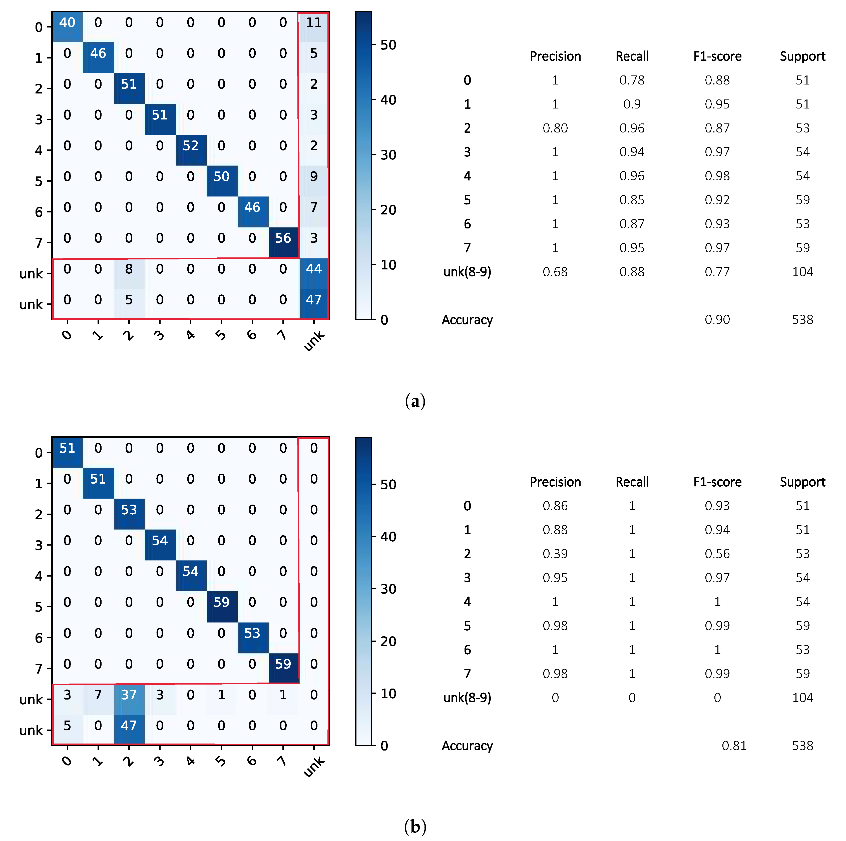
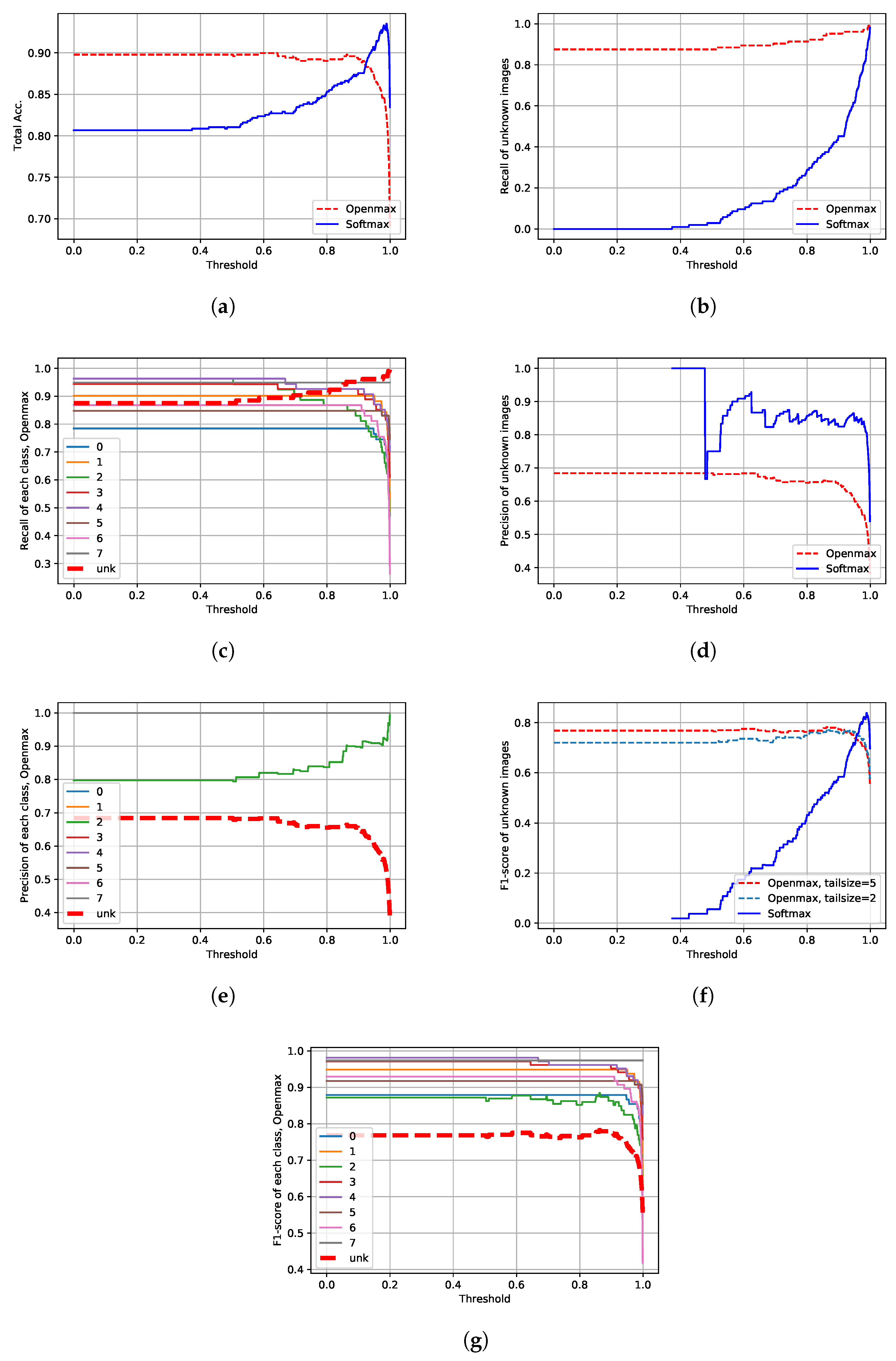
3.3. Classification Results: Openmax vs. Softmax

In this section, considering the performance indexes introduced in Section 2.3.3, the classification results of Openmax and Softmax are deeply analyzed. The confusion matrix and the corresponding classification reports obtained by using the Openmax approach when η = 5 are shown in Figure 5a, whereas those of the Softmax classifier are shown in Figure 5b. It can be seen that Softmax correctly classifies all the test images from classes 0 to 7 but it is not able to detect the unknowns. In fact, the images from classes 8 and 9 are classified as class 2, since they have a higher degree of similarity with this class, as can also be seen in Table 5. Note that the last column in the confusion matrices, i.e., class support size, represents the number of test images in the corresponding class. The term “support” is used by scikit-learn library [37], which is a widely used library in the machine learning community for different applications such as classification, regression [38] and so on. In addition, in order to show the discrimination between known and unknown classes clearly, a red box over unknown classes has been drawn.
To further improve the capability of classifiers to reject the unknown images, a threshold has been applied to their scores. The total accuracy of both Softmax and Openmax under different thresholds is shown in Figure 6a. Moreover, from Figure 6a, it can be noted that a threshold λ 0.38 for Softmax and λ 0.5 for Openmax does not produce any change in the total accuracy. When λ 0.5 , Openmax starts rejecting known images, while most of the unknown images were already rejected correctly. On the other hand, by increasing the threshold on Softmax, unknown images start to be rapidly rejected. Note that the Softmax scores are very close to 1, even in the case of unknown images. To achieve a comparable rejection performance with Openmax, the threshold on Softmax must be chosen carefully in the range of λ ( 0.9 , 1 ) . Setting such a threshold is not easy, since the performance changes very quickly in this range and degrades when the threshold is too close to one. An incorrect value of the threshold may result in poor total accuracy. Conversely, the Openmax approach does not necessarily need a threshold, as it has the total accuracy equal to 90 % even when λ = 0 .
Additionally, Figure 6b shows the R e performance index for the two unknown classes and further confirms the Softmax and Openmax behaviors against the unknown targets. Softmax starts rejecting images of classes eight and nine by λ 0.38 . On the other hand, 87.5 % of the unknown images are rejected by Openmax even by λ = 0 , and Openmax rejects the remaining unknown images by λ 0.5 . As the threshold approaches 1, the R e of the unknown set also tends to 100 % , since all the images in classes 8 and 9 will be marked as unknown by both classifiers. The R e of all the classes, including known and unknown ones, using the Openmax approach are shown in Figure 6c. It is possible to note that the R e values of the known classes are all in the range of ( 79 % , 95 % ) . Moreover, the higher the threshold, the lower the R e of the known classes and the higher the R e of the unknown class.
Turning our attention to the precision index, Figure 6d shows the P r of the unknown class. In particular, we can see from the Openmax diagram (the red curve) that P r remains constant at 68 % as long as the threshold does not exceed 0.5 . Subsequently, it begins to decrease as a threshold larger than 0.5 is used and more images from known classes are rejected. Differently, we can see from the Softmax diagram that using thresholds between 0.38 and 0.48 , the P r is equal to 100 % . Next, when λ 0.48 , the P r is unstable and changes in the range ( 75 % , 92 % ) . Finally, when λ approaches 1, both classifiers tend to the same value, P r = 104 538 19.3 % . Note that the blue curve is not drawn for thresholds lower than 0.38 , as we would obtain 0 0 in Equation (4), which is due to the inability of the Softmax classifier to reject unknown images by such thresholds. Let us now evaluate the P r of Openmax in known and unknown classes as shown in Figure 6e. We can see that apart from class 2 and U n k , the P r of other classes is 100 % and the threshold does not have any influence on them. The dissimilar behavior of class 2 compared to the other known classes is due to the fact that when unknown images are misclassified, they are assigned to the 2 class. However, by increasing the threshold, the P r of this class increases and tends gradually to 100 % .
Taking both P r and R e of the unknown classes into account, it is possible to calculate the F1-score of unknown images, which is another informative diagram shown in Figure 6f. This diagram shows that using a threshold on Softmax increases the F 1 of the unknown class. Conversely, applying a threshold on Openmax does not severely affect F 1 as long as the threshold does not exceed 0.9 . Similar to R e and P r , the behavior of the F 1 also depends on the tail size. For showing this, the F 1 obtained using a tail size of η = 2 has been added to the same plot. In Figure 6g, the F 1 diagram is shown also for the remaining classes using Openmax with η = 5 .
To better analyze the Openmax performance, other experiments have been conducted by changing the unknown classes. However, to limit the number of all possible combinations of known and unknown classes, only class 8 has been changed in each experiment. Therefore, beside the case of U n k = ( 8 , 9 ) , eight different experiments have been conducted in which U n k = ( k , 9 ) where k = 0 , 1 , 2 , , 7 . Obviously, every time the unknown class changes, the target labels need to be changed. For instance, when k = 3 , the classes are labeled as shown in Figure 7, and the same network is trained again with the new training set.
The metrics t r a i n i n g a c c u r a c y , t r a i n i n g l o s s , v a l i d a t i o n a c c u r a c y and v a l i d a t i o n l o s s of each of the nine scenarios are shown in Figure 8a,d to demonstrate that the network converges and it is not overfitted. The confusion matrices and classification reports of these nine scenarios are illustrated in Figure 9. It can be seen that the highest and the lowest accuracies are achieved, respectively, in the case of U n k = ( 6 , 9 ) and U n k = ( 1 , 9 ) . The average A c of all scenarios here is 85.9 % . The highest and the lowest R e of the unknown class are R e U n k ( 6 , 9 ) = 88 % and R e U n k ( 5 , 9 ) = 52 % , respectively. The average R e of the unknown class is 72.8 % . In order to make the comparison fair, all the results shown here were obtained by setting the tail size equal to 5 for each experiment. It is highly likely that the results would be further improved by adapting the tail size in each experiment.

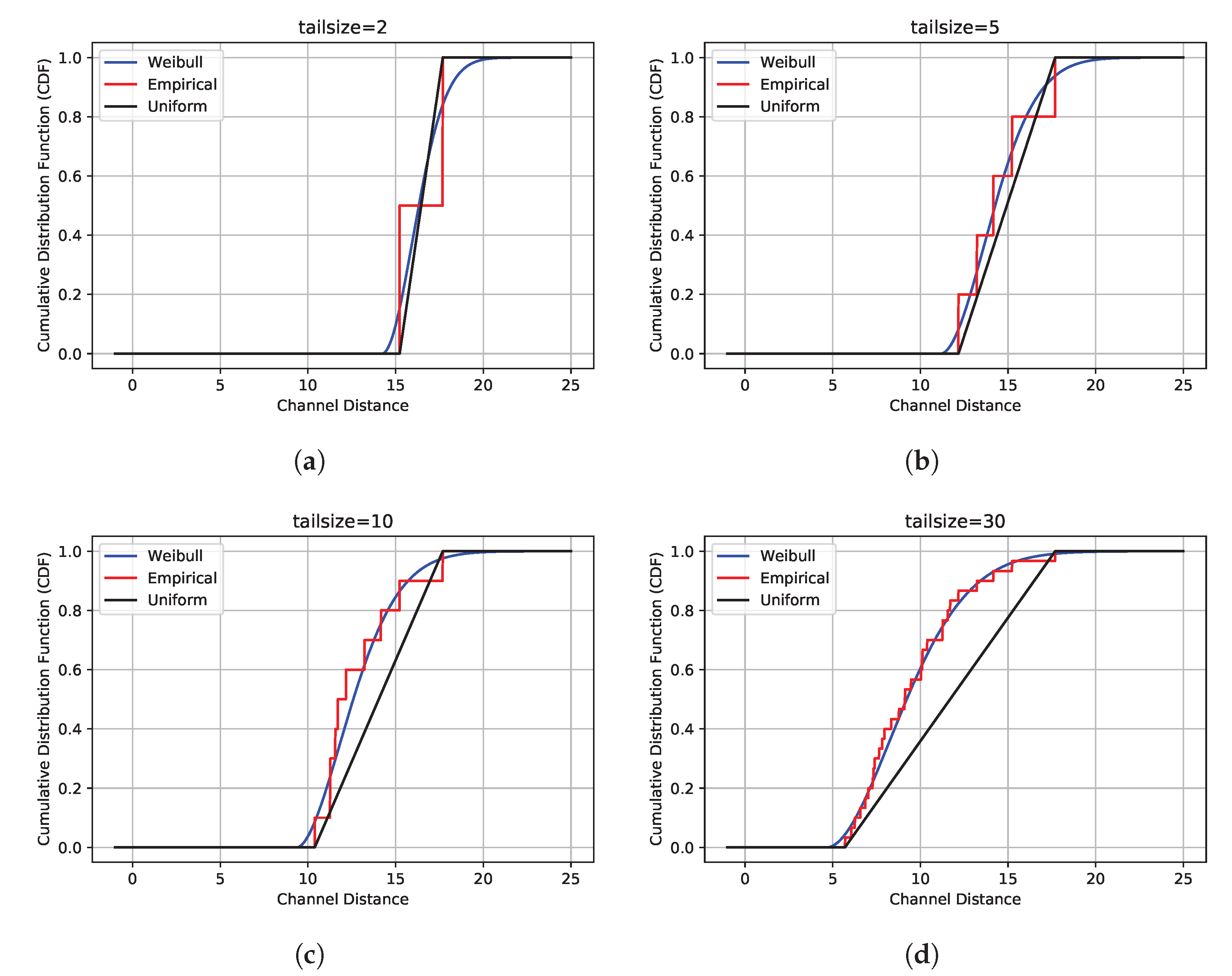
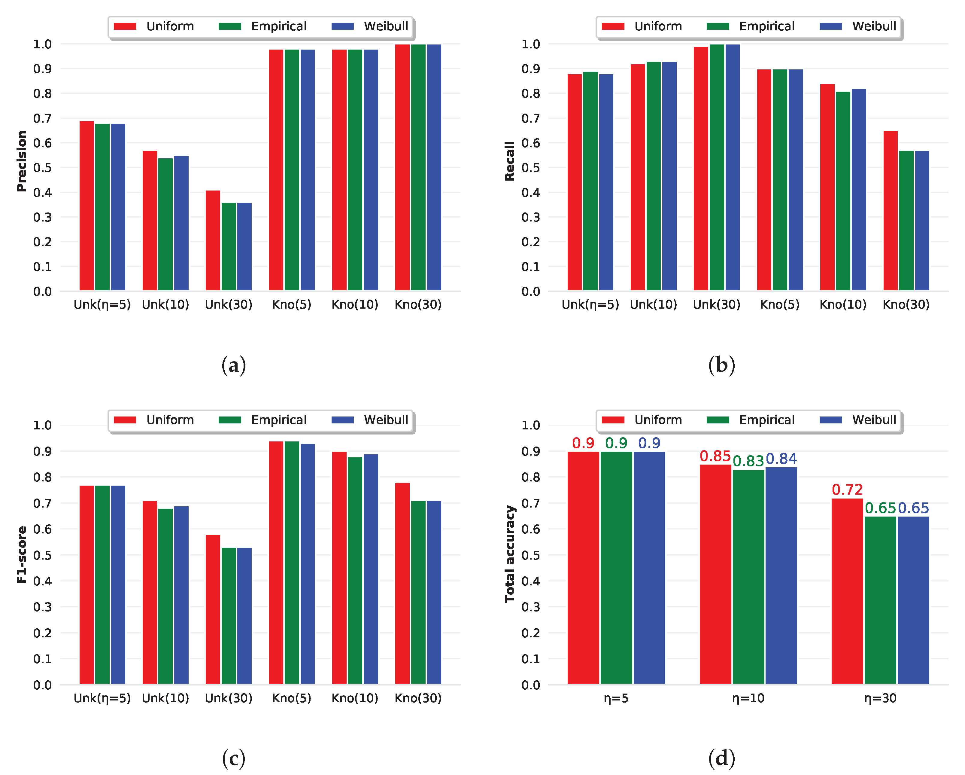
3.4. Statistical Analysis: The Effects of the Tail Size and of the CDF Type on Openmax

In this section, the effects of the tail size and the CDF type on the Openmax classification performance are deeply analyzed. Considering all the training images in class 0, the histogram of Euclidean distances between all AVs R 1 × 8 and the MAV R 1 × 8 of this class is shown in Figure 10. As previously mentioned, the η largest Euclidean distance values are used to fit a Weibull distribution. The choice of tail size is analyzed first. In particular, three different tail size values have been considered, and the relative Weibull CDFs are shown in Figure 11. More specifically, the green, orange and blue lines have been obtained using tail sizes equal to 40, 10, and 2, respectively. As it can be observed, the effect of decreasing the tail size reflects mostly a shift of the CDF toward the right direction, i.e., higher values of C D . To better understand the effect of such behavior, let us reconsider the aforementioned test image from class 0. The channel distance between the AV of this image and MAV of class 0 (the first row of Table 3) is C D = 5.53 as shown in Table 4. By looking at Figure 11, it is easy to observe that the Weibull function on this point is equal to 0 when the tail size is either 10 or 2. As a consequence, the corresponding w will be 0. Instead, when using the tail size of 40, Weibull CDF on C D = 5.53 gives a value greater than 0. This sets the corresponding w to 0.213, and since the corresponding element in AV is very large, 22.38 , a considerable amount of that AV score is subtracted and reserved for the unknown class. As a consequence, by using a tail size equal to 40, Openmax classifies this image as an unknown image with 80.4 % certainty. As a general rule, the larger the C D , the larger the w, and it means a higher probability of being recognized as an unknown. It can be concluded that the tail size plays an important role in the Openmax performance and it should be properly chosen, taking into consideration the available training set and the desired classifier performance to detect the unknowns. In fact, small tail size values mean a reduced capability in the detection of the unknowns. Conversely, large tail size values imply an improved capability in the detection of the unknowns but in some cases to the detriment of the known classes and resulting in lower total accuracy.
Another point to take into consideration is the choice of the probability function. The original Openmax classifier [18] uses the Weibull CDF. We analyze two other CDFs in this part, namely Uniform and Empirical distributions, to understand how much the CDF shape affects the Openmax performance. The mathematical expressions of probability and cumulative of the Uniform distribution are shown in (9) and (10), respectively.
f ^ ( x ) = 1 b a a x b 0 e . w
F ^ ( x ) = x a b a a x b 0 x a 1 x b
In this regard, a x b in each class, which are used for tail-fitting, are the Euclidean distances between all AVs of the class and their own MAV, whereas b a + 1 is the tail size. The Empirical cumulative distribution function, from M-ordered independent observations of X 1 < X 2 < X 3 < < X M , can be defined as [39]:
F ^ ( x ) = k M X k x < X k + 1 0 x X 1 1 x X M
F ^ ( x ) is in fact the consistent estimator of the true F ( x ) , since when the number of observations tends to infinity, F ^ (x) converges to F(x) for all x [40]. In our experiment, M corresponds to the tail size and values of X 1 x X M in each class, which denotes the Euclidean distance between all AVs of that class and their own MAV. The CDFs of the three models computed with tail size η = [ 2 , 5 , 10 , 30 ] are shown in Figure 12.
Note that in this scenario, η = 5 is optimal, and η = 10 is reasonable, while η = 2 and η = 30 are inserted to highlight the differences and similarities between the CDFs using extreme values of η .
It can be seen that when η is small, the difference between the CDFs is not prominent. The Uniform model can be considered as a linear approximation, while the Empirical model acts similar to the zero-order hold approximation of the standard Weibull CDF. However, by increasing the tail size ( η ), we can see that the Empirical CDF approaches the Weibull model asymptotically and the Uniform distribution deviates from the other two CDFs and gives smaller CDF values. Therefore, smaller values of w are expected from Uniform CDF, and this means a reduced sensitivity toward unknown targets.
The behavior of the Openmax performance against tail size and CDF models has been numerically assessed by means of diagrams shown in Figure 13. The terms Kno and Unk in Figure 13, which are used for the sake of brevity, refer to the known and unknown classes, respectively. In fact, Kno denotes the weighted average of parameters, i.e., R e , P r , and F 1 , over all known classes. The value of the tail size is also shown in parenthesis. It is possible to note that by increasing the tail size, the R e of the unknown class increases, while its P r decreases. Therefore, the classifier identifies a larger number of inputs as unknown independently of the CDF model. Interestingly, when η = 30 , the results of the Empirical and Weibull models are very similar, both having A c = 65 % , confirming that for a large tail size, the Empirical CDF approaches the Weibull CDF, whereas the Uniform outperforms the others having A c = 72 % . In this scenario, according to the total accuracy, the Uniform model is recommended independently of the tail size. However, the CDF model type has less impact on the classifier performance compared with the tail size choice.

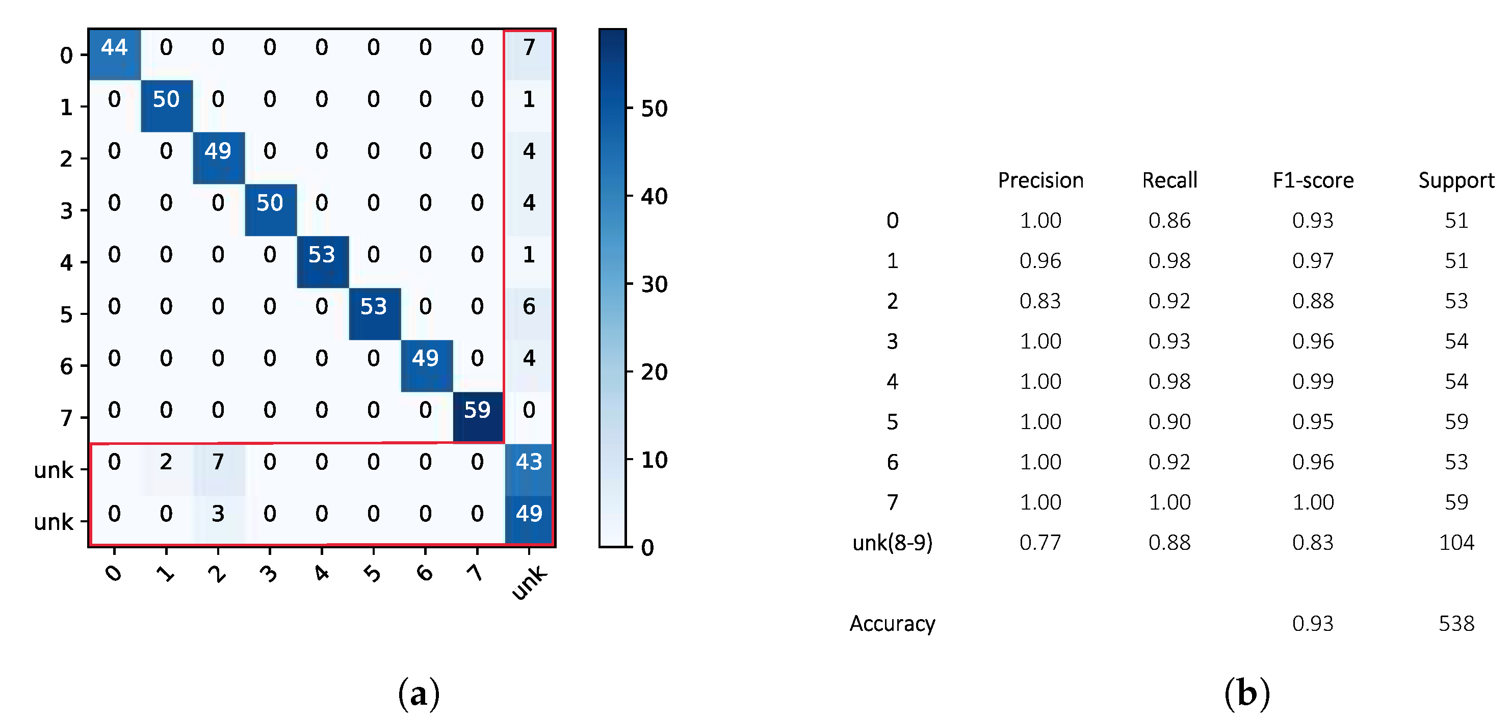
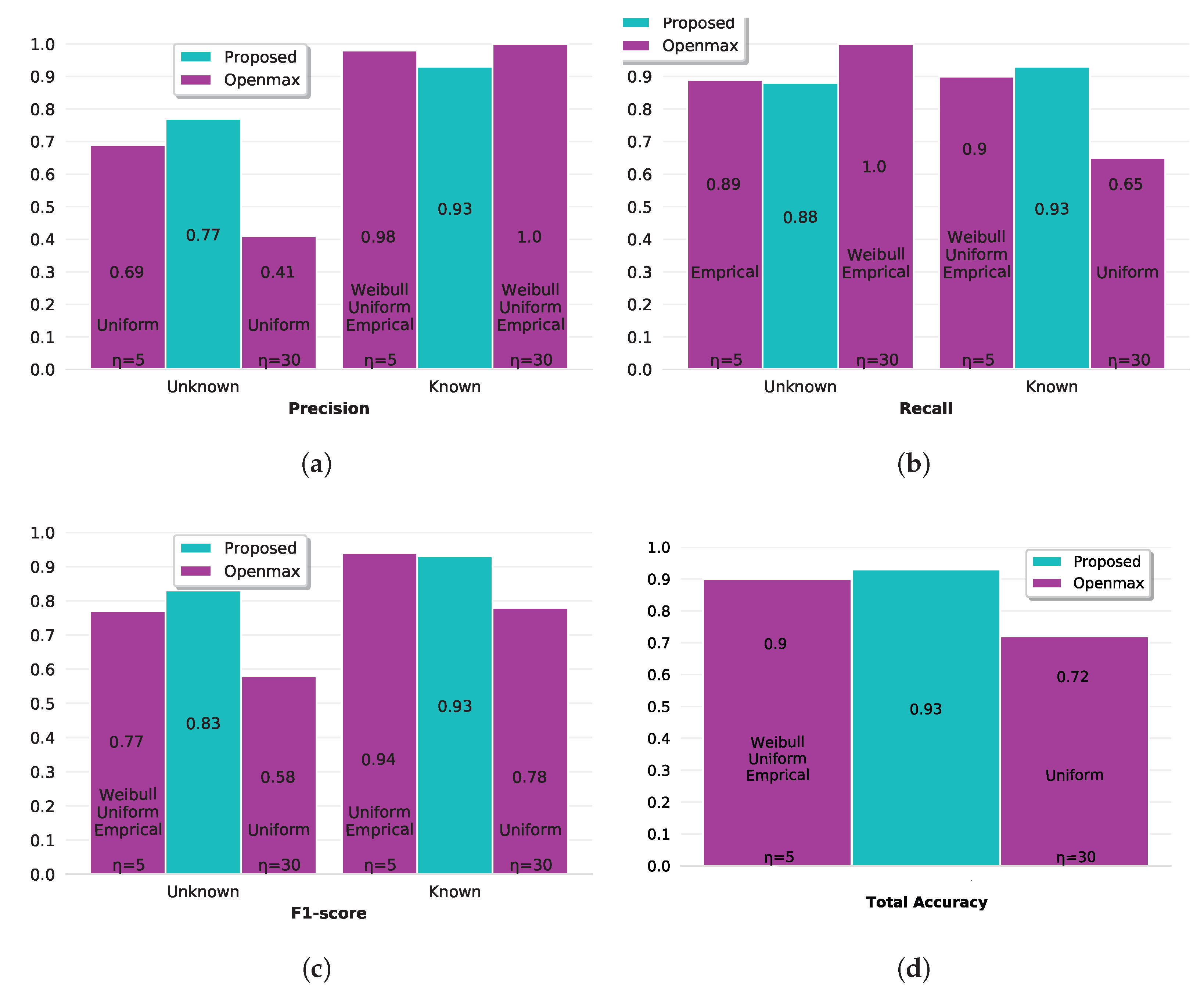
3.5. The Proposed Approach

In this part, we present the results achieved by our proposed PS-based approach that has been described in Section 2.2. The confusion matrix along with the performance indexes of the proposed PS-Openmax for the same scenario of Figure 5, i.e., when classes eight and nine are considered unknown, are shown in Figure 14.
We can notice that the total accuracy of the proposed approach is 3% higher than that of the original Openmax in Figure 5a.

4. Discussion

The salient features of the proposed approach are the use of a vector form supplementary activation function and interrelations between channel distances. Note that since the tail-fitting procedure is omitted in the PS-Openmax, there is no need to select and calibrate tail size and statistical distribution type. Moreover, N α is equal to the number of known classes, so we do not need any a priori information to limit the number of changeable neurons of AV. Therefore, all of AV’s elements can easily be modified while the second error shown in Figure 1, i.e., not rejecting an unknown image, is less likely to happen. This means that the proposed approach provides more robust performance.
Considering the performance indexes in Figure 14b, the weighted average of P r , R e , and F 1 for the known and unknown classes can be computed. For the sake of an easier comparison, we illustrate these weighted average parameters of the PS-Openmax in Figure 15, together with some selected ones from Figure 13, which were achieved by the original Openmax using η = 5 and η = 30 with the optimal statistical models. From Figure 15b, we can see that no matter what tail size and what distribution type are chosen in the original Openmax, the PS-based approach gives a higher R e in the known classes. This also corresponds to the higher P r in the unknown classes by the PS-based approach shown in Figure 15a. Taking both of these two parameters into account, we can see from the F 1 bar chart shown in Figure 15c that the PS-based approach outperforms the openmax classifier with η = 30 (and with the optimal distribution model that is Uniform) in both known and unknown classes. In fact, the scenario with η = 30 has been only conducted to have a higher recall in unknown classes, i.e., to reject all the unknown images. However, it rejects portions of the known images, as we can see the decreased R e of the known classes in Figure 15b or correspondingly the decreased P r of unknown classes in Figure 15a. In the end, the results shown in Figure 15d indicate that the proposed PS-Openmax outperforms the original Openmax classifier in terms of the total accuracy.

5. Conclusions

In this paper, we have proposed an approach to improve the performance of the Openmax classifier for the problem of open set recognition with radar images. The ability to detect unknown targets contributes to reducing the error rate and enhancing the precision when compared to the classical Softmax approach. This feature may be a desirable behavior, especially in military applications when false alarms need to be kept under control. In the proposed PS-based approach, for modifying the final activation vector of a well-trained CNN, we have exploited a vector form supplementary activation function, interrelations between channel distances, and the minimum channel distance. Although the proposed approach stems from the Openmax, it is technically different in some basic aspects such as substituting the most important part of Openmax, i.e., the tail-fitting procedure, for the aforementioned processing steps. Therefore, there is no necessity to select and calibrate the tail size and the statistical distribution type in the proposed approach. Furthermore, no restriction or in other words no a priori information is required about the number of changeable neurons in the final activation vector. Even by using different tail sizes and different statistical distribution models, which had not been addressed in the Openmax paper, the proposed approach outperforms the original Openmax classifier in terms of performance robustness and total accuracy.
This paper also provides a detailed description of the Openmax functioning that may be useful to an interested reader to try to implement it with any other DN for recognizing out-of-distribution inputs without necessarily imposing a threshold. In particular, the roles of both the tail size and the statistical model have been deeply investigated, showing that the tail size has to be carefully chosen during the model calibration phase. Conversely, the choice of the statistical model has less impact on the performance of the classifier compared with that of the tail size, meaning that the Weibull CDF is applicable to radar images as well. As a future research direction, combinations of the proposed approach and other DN is likely to produce high-performance classifiers.

Author Contributions

Conceptualization, E.G., S.G. and A.H.O.; methodology, A.H.O.; software, A.H.O. and S.G.; validation, E.G.; data curation, E.G.; writing, A.H.O., S.G. and E.G.; draft preparation A.H.O. and S.G.; review and editing, E.G., M.M., S.G. and A.H.O.; project administration, E.G. and M.M. All authors have read and agreed to the published version of the manuscript.

Funding

This research was funded by the National Inter-University Consortium for Telecommunications (CNIT) in Italy.

Acknowledgments

The authors would like to thank the anonymous reviewers for their time and helpful comments that improved the quality of this article.

Conflicts of Interest

The authors declare no conflict of interest.

References

  1. Huizing, A.; Heiligers, M.; Dekker, B.; de Wit, J.; Cifola, L.; Harmanny, R. Deep Learning for Classification of Mini-UAVs Using Micro-Doppler Spectrograms in Cognitive Radar. IEEE Aerosp. Electron. Syst. Mag. 2019, 34, 46–56. [Google Scholar] [CrossRef]
  2. Martorella, M.; Giusti, E.; Capria, A.; Berizzi, F.; Bates, B. Automatic Target Recognition by Means of Polarimetric ISAR Images and Neural Networks. IEEE Trans. Geosci. Remote Sens. 2009, 47, 3786–3794. [Google Scholar] [CrossRef]
  3. Martorella, M.; Giusti, E.; Demi, L.; Zhou, Z.; Cacciamano, A.; Berizzi, F.; Bates, B. Target Recognition by Means of Polarimetric ISAR Images. IEEE Trans. Aerosp. Electron. Syst. 2011, 47, 225–239. [Google Scholar] [CrossRef]
  4. Wagner, S.A. SAR ATR by a combination of convolutional neural network and support vector machines. IEEE Trans. Aerosp. Electron. Syst. 2016, 52, 2861–2872. [Google Scholar] [CrossRef]
  5. Ding, J.; Chen, B.; Liu, H.; Huang, M. Convolutional Neural Network With Data Augmentation for SAR Target Recognition. IEEE Geosci. Remote Sens. Lett. 2016, 13, 364–368. [Google Scholar] [CrossRef]
  6. Feng, S.; Ji, K.; Zhang, L.; Ma, X.; Kuang, G. SAR target classification based on integration of ASC parts model and deep learning algorithm. IEEE J. Sel. Top. Appl. Earth Observ. Remote Sens. 2021, 14, 10213–10225. [Google Scholar] [CrossRef]
  7. Yang, M.; Bai, X.; Wang, L.; Zhou, F. Mixed loss graph attention network for few-shot SAR target classification. IEEE Trans. Geosci. Remote Sens. 2022, 60, 1–13. [Google Scholar] [CrossRef]
  8. Wang, S.; Wang, Y.; Liu, H.; Sun, Y. Attribute-guided multi-scale prototypical network for few-shot SAR target classification. IEEE J. Sel. Top. Appl. Earth Observ. Remote Sens. 2021, 14, 12224–12245. [Google Scholar] [CrossRef]
  9. Li, Y.; Du, L.; Wei, D. Multiscale CNN based on component analysis for SAR ATR. IEEE Trans. Geosci. Remote Sens. 2022, 60, 1–12. [Google Scholar] [CrossRef]
  10. Lang, P.; Fu, X.; Feng, C.; Dong, J.; Qin, R.; Martorella, M. LW-CMDANet: A Novel Attention Network for SAR Automatic Target Recognition. IEEE J. Sel. Top. Appl. Earth Observ. Remote Sens. 2022, 15, 6615–6630. [Google Scholar] [CrossRef]
  11. Li, C.; Du, L.; Li, Y.; Song, J. A novel SAR target recognition method combining electromagnetic scattering information and GCN. IEEE Geosci. Remote Sens. Lett. 2022, 19, 1–5. [Google Scholar] [CrossRef]
  12. Zeng, Z.; Sun, J.; Han, Z.; Hong, W. SAR Automatic Target Recognition Method based on Multi-Stream Complex-Valued Networks. IEEE Trans. Geosci. Remote Sens. 2022, 60, 1–18. [Google Scholar] [CrossRef]
  13. Zhang, M.; An, J.; Yu, D.H.; Yang, L.D.; Wu, L.; Lu, X.Q. onvolutional neural network with attention mechanism for SAR automatic target recognition. IEEE Geosci. Remote Sens. Lett. 2020, 19, 1–5. [Google Scholar]
  14. Choi, J.H.; Lee, M.J.; Jeong, N.H.; Lee, G.; Kim, K.T. Fusion of Target and Shadow Regions for Improved SAR ATR. IEEE Trans. Geosci. Remote Sens. 2022, 60, 1–17. [Google Scholar] [CrossRef]
  15. Boult, T.E.; Cruz, S.; Dhamija, A.R.; Gunther, M.; Henrydoss, J.; Scheirer, W.J. Learning and the Unknown: Surveying Steps Toward Open World Recognition. Proc. AAAI 2019, 33, 9801–9807. [Google Scholar] [CrossRef]
  16. Hendrycks, D.; Gimpel, K. A baseline for detecting misclassified and out-of-distribution examples in neural networks. In Proceedings of the International Conference on Learning Representations, Toulon, France, 24–26 April 2017; pp. 1–12. [Google Scholar] [CrossRef]
  17. Guisti, E.; Ghio, S.; Oveis, A.H.; Martorell, M. Transfer Learning-Based Fully-Polarimetric Radar Image Classification with a Rejection Option. In Proceedings of the 18th European Radar Conference (EuRAD), London, UK, 5–7 April 2022; pp. 357–360. [Google Scholar]
  18. Bendale, A.; Boult, T.E. Towards open set deep networks. In Proceedings of the 2016 IEEE Conference on Computer Vision and Pattern Recognition (CVPR), Las Vegas, NV, USA, 27–30 June 2016; pp. 1563–1572. [Google Scholar] [CrossRef]
  19. Ge, Z.Y.; Demyanov, S.; Chen, Z.; Garnavi, R. Generative openmax for multi-class open set classification. arXiv 2017, arXiv:1707.07418. [Google Scholar]
  20. Geng, C.; Huang, S.-J.; Chen, S. Recent advances in open set recognition: A survey. IEEE Trans. Pattern Anal. Mach. Intell. 2020, 43, 3614–3631. [Google Scholar] [CrossRef]
  21. Zheng, Y.; Chen, G.; Huang, M. Out-of-domain detection for natural language understanding in dialog systems. IEEE ACM Trans. Audio Speech Lang. Process. 2020, 28, 119–1209. [Google Scholar] [CrossRef]
  22. Lee, K.; Lee, K.; Lee, H.; Shin, J. A simple unified framework for detecting out-of-distribution samples and adversarial attacks. In Proceedings of the 32nd International Conference on Neural Information Processing Systems, Montréal, QC, Canada, 3–8 December 2018; Volume 31, pp. 7167–7177. [Google Scholar]
  23. Inkawhich, N.A.; Davis, E.K.; Inkawhich, M.J.; Majumder, U.K.; Chen, Y. Training sar-atr models for reliable operation in open-world environments. IEEE J. Select. Top. Appl. Earth Observ. Remote Sens. 2021, 14, 3954–3966. [Google Scholar] [CrossRef]
  24. Guisti, E.; Ghio, S.; Oveis, A.H.; Martorella, M. Open Set Recognition in Synthetic Aperture Radar Using the Openmax Classifier. In Proceedings of the 2022 IEEE Radar Conference (RadarConf22), New York, NY, USA, 21–25 March 2022. [Google Scholar]
  25. Oveis, A.H.; Guisti, E.; Ghio, S.; Martorella, M. Extended Openmax Approach for the Classification of Radar Images with a Rejection Option. IEEE Trans. Aerosp. Electron. Syst. 2022. [Google Scholar] [CrossRef]
  26. The Air Force Moving and Stationary Target Recognition Database. Available online: www.sdms.afrl.af.mil/index.php?collection=mstar (accessed on 5 April 2014).
  27. Scheirer, W.J.; Rocha, A.; Micheals, R.J.; Boult, T.E. Meta-recognition: The theory and practice of recognition score analysis. IEEE Trans. Pattern Anal. 2011, 33, 1689–1695. [Google Scholar] [CrossRef] [PubMed]
  28. Chen, W.; Wang, Y.; Song, J.; Li, Y. Open set HRRP recognition based on convolutional neural network. J. Eng. 2019, 21, 7701–7704. [Google Scholar] [CrossRef]
  29. Lewis, B.; Scarnati, T.; Sudkamp, E.; Nehrbass, J.; Rosencrantz, S.; Zelnio, E. A SAR dataset for ATR development: The Synthetic and Measured Paired Labeled Experiment (SAMPLE). In Proceedings of the Algorithms for Synthetic Aperture Radar Imagery, Baltimore, MD, USA, 18 April 2019; pp. 39–54. [Google Scholar]
  30. Chen, S.; Wang, H. SAR target recognition based on deep learning. In Proceedings of the 2014 International Conference on Data Science and Advanced Analytics (DSAA), Shanghai, China, 30 October–1 November 2014; pp. 541–547. [Google Scholar]
  31. Du, K.; Deng, Y.; Wang, R.; Zhao, T.; Li, N. SAR ATR based on displacement- and rotation-insensitive CNN. Remote Sens. Lett. 2016, 7, 895–904. [Google Scholar] [CrossRef]
  32. Wang, L.; Bai, X.; Zhou, F. SAR ATR of ground vehicles based on ESENet. Remote Sens. 2019, 11, 1316. [Google Scholar] [CrossRef]
  33. Mossing, J.C.; Ross, T.D. Evaluation of sar atr algorithm performance sensitivity to mstar extended operating conditions. Proc. SPIE Int. Soc. Opt. Eng. 1998, 13, 554–565. [Google Scholar]
  34. Scheirer, W.J.; Rocha, A.d.; Sapkota, A.; Boult, T.E. Toward open set recognition. IEEE Trans. Pattern Anal. Mach. Intell. 2013, 35, 1757–1772. [Google Scholar] [CrossRef]
  35. Oveis, A.H.; Guisti, E.; Ghio, S.; Martorella, M. A Survey on the Applications of Convolutional Neural Networks for Synthetic Aperture Radar: Recent Advances. IEEE Aerosp. Electron. Syst. Mag. 2021, 37, 18–42. [Google Scholar] [CrossRef]
  36. Giannakopoulos, T.; Pikrakis, A. Introduction to Audio Analysis: A MATLAB® Approach; Academic Press: Cambridge, MA, USA, 2014. [Google Scholar]
  37. Pedregosa, F.; Varoquaux, G.; Gramfort, A.; Michel, V.; Thirion, B.; Grisel, O.; Blondel, M.; Prettenhofer, P.; Weiss, R.; Dubourg, V.; et al. Scikit-learn: Machine learning in Python. J. Mach. Learn. Res. 2011, 12, 2825–2830. [Google Scholar]
  38. Oveis, A.H.; Giusti, E.; Ghio, S.; Martorella, M. CNN for Radial Velocity and Range Components Estimation of Ground Moving Targets in SAR. In Proceedings of the 2021 IEEE Radar Conference (RadarConf21), Atlanta, GA, USA, 7–14 May 2021. [Google Scholar]
  39. Coles, S. An Introduction to Statistical Modeling of Extreme Values; Springer: New York, NY, USA, 2001. [Google Scholar]
  40. Van der Vaart, A.W. Asymptotic Statistics; Cambridge University Press: Cambridge, UK, 1998. [Google Scholar]
Figure 1. Openmax limitations, source of errors.
Remotesensing 14 04665 g001
Figure 2. The overall framework of the PS-based Openmax classifier: (a) Calculation of MAVs. (b) Activation vector of the test image and Channel Distance vector. (c) Modification of the AV.
Remotesensing 14 04665 g002
Figure 3. Electro-optical images corresponding to the MSTAR dataset used in this paper; (a) BTR70, (b) M1, (c) M2, (d) M35, (e) M60, (f) M548, (g) T72, (h) ZSU23-4, (i) 2S1, (j) BMP2.
Remotesensing 14 04665 g003
Figure 4. Testing the Openmax approach with a very different image in comparison with the other open set images in MSTAR radar dataset.
Remotesensing 14 04665 g004
Figure 5. Confusion matrix and the corresponding classification reports using (a) Openmax, (b) Softmax.
Remotesensing 14 04665 g005
Figure 6. Applying a threshold on the output scores of the classifiers. (a) Total accuracy of Softmax and Openmax ( η = 5); (b) Recall of the unknown images using Softmax and Openmax ( η = 5 ); (c) Recall of the known classes together with the unknown one using Openmax ( η = 5); (d) Precision of unknown images using Softmax and Openmax ( η = 5 ); (e) Precision of the known classes together with the unknown one using Openmax approach; ( η = 5) (f) F1-Score of unknown images using Softmax and Openmax ( η = 2 , η = 5 ); (g) F1-Score of the known classes together with the unknown one using Openmax ( η = 5).
Remotesensing 14 04665 g006
Figure 7. How to rearrange class labels in order to have a different Unk class and generalize the experiment.
Remotesensing 14 04665 g007
Figure 8. Metrics used to demonstrate the goodness of fitting: (a) training accuracy, (b) training loss, (c) validation accuracy, (d) validation loss.
Remotesensing 14 04665 g008aRemotesensing 14 04665 g008b
Figure 9. Confusion matrices and classification reports of Openmax when the first unknown class is changed while the second one is fixed: from (ai) correspond to scenarios of having two unknown classes of (k,9) where k = 0, …, 8.
Remotesensing 14 04665 g009aRemotesensing 14 04665 g009b
Figure 10. The histogram of Euclidean distances between AVs and MAV of class 0 of training images.
Remotesensing 14 04665 g010
Figure 11. CDF of Weibull function fitted to η = 2, 10, 40 largest distance values between AVs and MAV of the class zero in the training images.
Remotesensing 14 04665 g011
Figure 12. Three different CDFs, i.e., Uniform, Empirical and Weibull distributions, fitted to the tails of distance values of images in class zero (a) η = 2 , (b) η = 5 , (c) η = 10 , (d) η = 30 .
Remotesensing 14 04665 g012
Figure 13. Classification reports obtained by η = ( 5 , 10 , 30 ) using Uniform, Empirical and Weibull CDFs: (a) Precision, (b) Recall, (c) F1-score, and (d) Total accuracy.
Remotesensing 14 04665 g013
Figure 14. The results of the proposed PS-Openmax approach: (a) the confusion matrix and (b) the corresponding classification metrics.
Remotesensing 14 04665 g014
Figure 15. Comparison between the proposed PS-Openmax approach and the original Openmax classifier: (a) Precision, (b) Recall, (c) F1-Score, and (d) Total accuracy.
Remotesensing 14 04665 g015
Table 1. Structure of the CNN.
LayerNameOutput SizeAct. Func.Param.
0Input64 × 64 × 1-0
1Conv164 × 64 × 16ReLU160
2MaxPooling132 × 32 × 16-0
3Conv232 × 32 × 16ReLU2320
4MaxPooling216 × 16 × 16-0
5Conv316 × 16 × 64ReLU25,664
6Flattening16,384-0
7FC150-819,250
8FC28-408
9Classifier8Softmax0
Table 2. MSTAR dataset.
LabelNameSerial NumberN TrainN Test
known0BTR 70C714151
1M10AP00N7851
2M2MV02GX7553
3M35T8397554
4M60333612254
5M548C245HAB6959
6T728125553
7ZSU23-4D0811559
unknown82S1B01052
9BMP29563052
total---630538
Table 3. Matrix M shows the mean values of AVs in each class.
Class
025.87740.59252314.02069.63976−19.11180.5058121.15104−13.4153
1−9.3734216.43022.61673−1.712365.15303−2.035164.97492−0.208769
23.532984.817116.9942−0.0574321−5.61154−1.52066.13859−8.09596
3−3.972350.510664−5.9503424.1043−6.4027611.65054.77716−2.15785
4−13.03759.81838−1.278910.35065718.859−6.834636.974380.575225
5−5.169360.803306−4.1996118.1028−12.615629.31764.19841.5873
6−4.983375.713934.890131.97763.75332−3.9214315.4734−7.05234
7−9.568595.69773−2.108841.12619−0.9579032.00531−4.0433519.9382
Table 4. Intermediate parameters of the Openmax algorithm given an input image from the class 0.
Channel01234567 
Channel Distance ( C D )5.5345.8224.6341.7755.7948.6439.1551.35 
w = Weibull CDF (on C D )010.9911111 
Softmax0.99 5.68 × 10 10 2 × 10 4 5.79 × 10 7 6.01 × 10 18 2.39 × 10 11 1.41 × 10 9 2.52 × 10 15  
α 10.50.8750.750.1250.3750.6250.25 
AV22.381.0913.928.01−17.27−2.071.99−11.23 
modAV (@ line 8 Algorithm 2)22.380.551.742−15.11−1.30.75−8.43 
AV-modAV00.5412.186.01−2.15−0.771.24−2.8 
modAV (@ line 10 Algorithm 2)22.380.551.742−15.11−1.30.75−8.4314.24
Openmax0.99 3.28 × 10 10 1.08 × 10 9 1.41 × 10 9 5.2 × 10 17 5.19 × 10 11 4.03 × 10 10 4.17 × 10 14 2.94 × 10 4
Table 5. Intermediate parameters of the Openmax algorithm given an unknown input radar image.
Channel01234567
Channel Distance ( C D )19.1544.9220.2645.4253.9951.0434.555.67
w = Weibull CDF (on C D )0.9910.9911111
Softmax 8.35 × 10 3 3.09 × 10 10 0.991 1.2 × 10 8 1.87 × 10 15 1.43 × 10 9 1.01 × 10 4 8.8 × 10 18
α 0.8750.37510.6250.250.50.750.125
AV16.17−0.9320.952.72−12.940.5911.76−18.31
modAV (@ line 8 Algorithm 2)2.12−0.580.011.0−9.710.32.94−16.02
AV-modAV14.05−0.3520.941.7−3.230.298.82−2.2
modAV (@ line 10 Algorithm 2)2.12−0.580.011.0−9.710.32.94−16.0239.94364
Openmax 3.75 × 10 17 2.5 × 10 18 4.52 × 10 18 1.24 × 10 17 2.72 × 10 22 6.05 × 10 18 8.51 × 10 17 4.94 × 10 25 0.99
Publisher’s Note: MDPI stays neutral with regard to jurisdictional claims in published maps and institutional affiliations.

