Article

An Efficient Feature Extraction Network for Unsupervised Hyperspectral Change Detection

1
School of Electronic Engineering, Xidian University, Xi’an 710071, China
2
School of Computer Science and Technology, Xidian University, Xi’an 710071, China
*
Author to whom correspondence should be addressed.
Remote Sens. 2022, 14(18), 4646; https://doi.org/10.3390/rs14184646
Submission received: 31 July 2022 / Revised: 4 September 2022 / Accepted: 13 September 2022 / Published: 17 September 2022
(This article belongs to the Special Issue State-of-the-Art Remote Sensing Image Scene Classification)

Abstract

:
Change detection (CD) in hyperspectral images has become a research hotspot in the field of remote sensing due to the extremely wide spectral range of hyperspectral images compared to traditional remote sensing images. It is challenging to effectively extract features from redundant high-dimensional data for hyperspectral change detection tasks due to the fact that hyperspectral data contain abundant spectral information. In this paper, a novel feature extraction network is proposed, which uses a Recurrent Neural Network (RNN) to mine the spectral information of the input image and combines this with a Convolutional Neural Network (CNN) to fuse the spatial information of hyperspectral data. Finally, the feature extraction structure of hybrid RNN and CNN is used as a building block to complete the change detection task. In addition, we use an unsupervised sample generation strategy to produce high-quality samples for network training. The experimental results demonstrate that the proposed method yields reliable detection results. Moreover, the proposed method has fewer noise regions than the pixel-based method.

Graphical Abstract

1. Introduction

In recent years, change detection (CD) has attracted increasing interest due to its wide range of possible applications [1,2,3,4,5,6,7], such as urban development, land cover monitoring, natural disaster detection, and ecosystem monitoring. CD aims to identify the changing area by comparing two images of the same place taken at two different times [8].
With the rapid development of remote sensing technologies, obtaining large numbers of hyperspectral images (HSIs) for CD has become much easier. HSIs have more detailed spectral patterns and textural information than other remote sensing images, such as RGB images, multispectral images (MSIs), and synthetic aperture radar (SAR) images [9,10,11]. Consequently, HSIs have the potential to identify more subtle variations [12], and the detailed composition of different categories are effectively distinguished. However, the high-spatial-resolution characteristics of HSIs will also bring challenges to the CD feature-extraction network. In summary, there are two reasons for this. Firstly, labeled HSI datasets for CD tasks are lacking, making it difficult to train a deep feature extraction network using a supervised learning algorithm. Secondly, because the spectral bands of HSIs are relatively dense, the image-processing methods for multispectral or optical remote sensing images cannot be directly migrated to effectively mine the spectral information of HSI.
Focusing on the challenges mentioned above, some new advances have recently been achieved in improving HSI-CD feature extraction. Among them, principal component analysis (PCA) [13] is the most commonly used component, which can map the high-dimensional information of HSI to the low-dimensional space. Specifically, in order to acquire the mapping features, take the HSI of H × W × C as input, and obtain the coefficient of the C channel to generate the H W × H W covariance matrix. According to this covariance matrix, the mapping transformation operation of each H × W layer is obtained, and this transformation is linear. Another component worth mentioning is compressed change vector analysis ( C 2 VA) [14], which is inspired by metric learning and can be implemented in two steps. First, it calculates the spatial Euclidean Distance between each 1 × 1 × C pixel and clusters each pixel with the idea of metric learning. Second, it calculates the spatial angle of each pixel and establishes the phase relationship between different pixels to classify different categories. This transformation is non-linear. The above two methods are the classic work of change detection, and many subsequent works have been improved based on them, such as sequential spectral change vector analysis ( S 2 CVA) [15], Robust Change Vector Analysis (RCVA) [16]. However, all of the above methods use the statistical information of all pixels in a single channel to determine the importance of the current channel and then compress high-dimensional features into a low-dimensional feature space. Differing from previous work, we consider how to make each pixel select the optimal channel for the final task, and integrate these channels into a new feature channel, to release the potential of the maximally effective information.
Compared with the fully convolutional network (FCN) and convolutional neural network (CNN), the recurrent neural network (RNN) can identify the data association between sequence information. Applying the RNN structure to the feature extraction of HSIs has the following advantages:
  • The sequence information of HSIs can be retained. The previous band selection method will destroy the time sequence of feature space, while RNN will give each sequence a new weight to maintain the spectral information, and the importance of each spectral can be enhanced or inhibited by the weights.
  • The sequence process of RNN is beneficial when reducing the redundant information in HSI. As the features between adjacent channels of a hyperspectral channel are similar, it is even possible to predict the current channel’s information from the previous channel’s features. RNN can make full use of this feature to filter redundant information.
Based on the two superiorities mentioned earlier, this paper develops a new feature extraction network based on the hybrid CNN and RNN for HSI-CD tasks. The main contributions are summarized as follows:
  • A feature extraction network based on RNN is proposed, which can better retain the time sequence information of HSIs and is also more conducive to filtering out redundant information.
  • The subsequent CNN structure utilizes the spectral information of adjacent regions to suppress noise and improve change detection results.
  • For binary change detection, our method can extract the most relevant feature channel for each pixel. It can relieve the mixture problem of remote sensing image change detection.
The rest of this paper is organized as follows. Section 2 gives a brief review of the related work. Section 3 introduces the preliminary knowledge about our method and describes our proposed method in detail. The datasets and comprehensive experimental results are shown in Section 4. The discussion of the effectiveness of RNN and the setting of hyperparameters is presented in Section 5. Finally, in Section 6, we provide a summary of this paper.

2. Related Work

The current CD methods used for HSIs can roughly be divided into four categories: change vector analysis, spectral unmixing, deep neural network methods, and optimized pseudo-label generation methods.

2.1. Change Vector Analysis (CVA) Based Methods

The change vector detection method [17] is the pre-classification change detection. A spectral change vector between the two time phases is computed to show the degree of change. Bruzzone et al. [18] designed an unsupervised change detection algorithm based on CVA. The paper by Bovolo et al. [19] addressed unsupervised change detection by proposing a proper framework for a formal definition and a theoretical study of the CVA technique. Thonfeld et al. [16] proposed an approach called RCVA, aiming to mitigate the effects of differences in viewing geometries or registration noise. The CVA technique was also used in [20,21]. Furthermore, Gong et al. [22] proposed a reformulated fuzzy local-information C-means clustering method for classifying changed and unchanged regions in the fused difference image. Celik et al. [23] proposed the use of a PCA algorithm to generate feature vector spaces and K-Means clustering using Euclidean distance for change detection. Nielsen [24] proposed an iterative weighted multivariate change detection (IR-MAD) algorithm based on the MAD, which extends the MAD by iterating the weights of different observations. Tang et al. [25] used a pixel ratio approach to identify the range of change. They determined the change type in the classification map by comparing object-based classifications. Rawashdeh and Bashir [26] used the pixel-by-pixel method of differential change detection to identify and evaluate newly implemented irrigation areas. All the above literature examples are classic methods in the change detection field, and they promote the development of change detection. However, there are still some challenges when applying the above methods to HSI-CD.

2.2. Spectral Unmixing Based Methods

To solve this mixture problem, which is caused either by the limited spatial resolution of the sensors, which includes different objects in a single pixel, or by the combination of the distinct materials into a homogeneous mixture, spectral unmixing techniques were developed. Liu et al. [27] proposed an unsupervised multitemporal spectral unmixing for detecting multiple changes in HSI. In literature [28], subpixel change detection is addressed for a case study using abundance and slope features. Ertürk et al. [29] exploited dictionary pruning for the first time in HSI-CD using sparse unmixing. Furthermore, in [30], Ertürk et al. investigated CD for HSI by spectral unmixing and systematically presented the advantages that can be gained by using such a method. Li et al. [31] presented an integrated change detection method based on multi-endmember spectral unmixing, joint matrix and CNN (MSUJMC) for HSI. Considering the endmember spectral variability, they obtained more reliable endmember abundance information with multi-endmember spectral unmixing (MSU). Due to the highly mixed nature of pixels in HSI data, instead of directly using the raw pixel for anomaly detection, Qu et al. [32] proposed an algorithm that applies spectral unmixing to obtain the abundance vectors and uses these vectors for anomaly detection. Seydi et al. [33] presented a new hyperspectral change detection framework based on a robust binary mask and convolutional neural network. In this research, they generated pseudo-training data based on an image-differencing algorithm and spectral unmixing manner for multiple change detection. In [34], the authors proposed a novel technique for unsupervised change detection in multitemporal satellite images using principal component analysis and K-Means clustering. Although the method based on spectral unmixing can solve the mixture effect, it still does not select the best channel for each pixel according to different categories.

2.3. Deep Neural Network Based Methods

Recently, researchers have begun to consider the use of deep learning methods to extract features for HSI-CD. Huang et al. [35] proposed a multi-temporal HSI-CD method based on tensor and deep learning to make full use of the underlying feature change information of HSI. Zhan et al. [36] trained a supervised siamese convolutional network, which learned to directly extract features from the image pairs. In the literature [37], Mou et al. embedded a recurrent neural network and a convolutional neural network into an end-to-end network, which focuses on analyzing temporal dependence and generating rich spectral-spatial feature representations in bi-temporal images. Ken et al. [38] proposed a novel change detection method that uses CNN features in combination with superpixel segmentation. Wang et al. [39] presented a faster, region-based convolutional neural network (Faster R-CNN) for the detection of high-resolution remote sensing image changes. Liu et al. [2] proposed an unsupervised deep convolutional coupling network for change detection, which is symmetrical, with each side consisting of one convolutional layer and several coupling layers. Wang et al. [12] introduced a General End-to-end Two-dimensional CNN (GETNET) framework for HSI-CD, in which they designed an effcient 2-D CNN structure to learn the discriminative features at a higher level. In order to better extract the discriminative CNN features, Li et al. [40] proposed a novel noise modeling-based unsupervised FCN framework for HSI-CD. However, most of the above literature only focuses on using the statistical information of each channel to determine the importance of the channel for feature selection. This will bring two problems: one is that each pixel does not select the optimal channel, and the other is that, for each category of tasks, the extracted features are not targeted, but some channel features are selected for the overall task. Our proposed HSI-CD feature extraction network based on RNN can solve these two problems very well.

2.4. Pseudo Label Generation Methods

Due to the difficulty of collecting change detection datasets and annotations, most of the current mainstream change detection techniques are based on unsupervised learning. During the unsupervised training of the network, the generation of pseudo-labels for the samples is an important research focus. The quality of the pseudo-labels determines the performance of the subsequent detection results. Li et al. [41] converged the similarity matrix of the initial features by deep belief network into two classes as a pseudo-label for global-local SPPNet training data. Gao et al. [42] used a logarithmic ratio operator and a hierarchical FCM classifier to generate pseudo-label training samples. Zhang et al. [43] proposed an automated method to detect changes in bi-temporal SAR images based on a pre-train scheme and the PCANet algorithm. They utilized the parallel FCM to produce three types of pseudo-label training pixels: changed, no-change and intermediate pixels. Liu et al. [44] applied a log-ratio algorithm to generate the pseudo labels, and then trained the network utilizing the change information extracted by the pretrained model and contained in the pseudo-labels. Zhou and Li [45] designed an image filter to control the usage of change information in the pseudo-labels in the network’s training process. Furthermore, they proposed a novel training strategy, named unsupervised self-training. The usage of the joint pseudo-labels can reduce the negative influence of errors in the single set of pseudo-labels.

3. Method

In this work, an effective feature extraction network for HSIs is proposed, where the sequence information of hyperspectral images can be retained and each pixel can select the optimal channel information. The proposed method is based on the hierarchical integration of the RNN and CNN, which are both the current state-of-the-art DNN architecture for temporal sequence processing. Concretely, a graph illustrating the presented method is shown in Figure 1, from which we can see that the proposed methodology contains three main parts: low-dimensional feature extractor, high-dimensional feature extraction module based on hybrid RNN and CNN, and the final, fully connected layer. The low-dimensional feature extractor and the hybrid feature learning module will be introduced in the next few sections.

3.1. Low-Dimensional Feature Extractor

CNN is a category of neural network that is mainly used to examine, recognize or classify images as it simplifies them for improved understanding. The advantage of CNN is that it requires less labor and pre-processing. Backpropagation is also a part of the learning procedure, making the network more efficient. The design is intimately related to MLP, as it consists of an input layer of neurons, multiple hidden layers, and an output layer. Each individual neuron in one layer is attached to each neuron in a subsequent layer.
As shown in Figure 1, in our model, we first apply a convolutional layer with size of 1 × 1 on an HSI to extract the shallow features. Then, a filter of size 3 × 3 is repeatedly applied to the sub-matrices of the input feature maps. It is worth noting that the size of the feature map, in this case, is H × W × 128 , meaning that we reduced the channels of the input image to 128 instead of 32 while keeping the length and width the same. This will eliminate the loss of temporal information caused by the CNN dimensionality reduction.The feature maps of two convolutional layers are calculated as follows:
X = Φ ( f c 2 3 × 3 ( Φ ( f c 1 1 × 1 ( x ) ) ) ) = Φ ( ω 2 ( Φ ( ω 1 ( x ) ) ) ) ,
where f c 1 1 × 1 and f c 2 3 × 3 stand for the convolutional kernel of size 1 × 1 ( 3 × 3 ) with channel c 1 ( c 2 ). Φ represents ReLu function and ω 1 and ω 2 are parameters of convolutional layers f c 1 1 × 1 and f c 2 3 × 3 , respectively.
It is important to state that, in addition to the two convolutional layers mentioned above, our model also has a separate convolutional layer following each RNN. The purpose is to better mix the sequence information extracted from the RNN for higher-level semantic representation.

3.2. Feature Learning of Hybrid RNN and CNN

Our initial assumption was to directly feed hyperspectral data with sequence information to an RNN. As depicted in [37], RNNs have been extensively deployed to deal with sequence data. This extracts both the temporal dependencies between data samples in a sequence and captures the most discriminative features for that sequence to execute various tasks. However, in actual operation, the RNN will be slower than the CNN due to the optimization problem of the parallel computing library. In the first few layers of the network, in order to improve the training speed, we first used the CNN for the dimensionality reduction of the data. Then, the RNN was utilized to capture the temporal information hidden in channels of feature maps generated by CNN for further processing. RNNs have the benefit of acquiring complex temporal dynamics over sequences in comparison to standard feedforward networks. Given an input sequence x 1 , x 2 , x T , an RNN layer calculates the forward sequence of the hidden states H = h 1 , h 2 , , h T by iterating from t = 1 to T:
h t = σ W i x i + W h h t 1 + b h ,
where W i is the weight matrix from input to hidden and W h is the weight matrix from hidden to hidden. In addition to the input x i , the hidden activation h t 1 of the former time step is fed to affect the hidden state of the current time step. In a bidirectional RNN, a recurrent external layer is used to evaluate the backward sequence of the hidden outputs H from t = T to 1.
h t = σ W i x i + W h h t 1 + b h .
In experiments, our model stacks two bidirectional recurrent layers if not specifically informed otherwise. At each time step t, the cascade of forward and backward hidden states h t , h t of the current layer is considered as the next recursive layer’s input. In this case, the output at each frame t is the conditional distribution p ( x t | x t 1 , , x 1 ) . For example, a polynomial distribution would be exported with a softmax activation function.
p x i , j = 1 x t 1 , , x 1 = exp w j h t / k = 1 K exp w k h t .
Furthermore, we can compute the probability of each sequence x by integrating these values using the following equation.
p x = t = 1 T p x t x t 1 , , x 1 .
The outputs of the convolutional layer following RNN are flattened and form a feature vector, which may then be used as the input of a fully connected network (see Figure 1).

3.3. Change Detection Head Based on Fully Connected Network

After the above feature extraction stage, the above module can perform feature extraction on the input hyperspectral images of different phases, respectively. For an input image patch of size 17 × 17 , a feature map pair of size 3 × 3 can be obtained. The feature map with a size of 3 × 3 can be considered a high-dimensional semantic information, representing the region in which the central pixel is located. Intuitively, we take the difference of the two obtained feature maps and expand the obtained result into a vector, which serves as a measure of the change value. Compared with the common CVA method, this method can reduce the dimension of the vector and suppress the overfitting of the network. Differing from the method based on pixel points, this method can better fuse the spatial information and spectral information of the region.
Referring to the common neural network structure design, we used three cascaded fully connected layers and ReLU as the activation function and the subsequent change detection head. Since the dataset is a change detection task for two types of changes, the last layer of the network contains only two neurons, representing the degree of activation for the categories of change and no change, respectively. The overall fully connected layer is used to classify the difference information and generate binary change detection results. Due to the high efficiency of the feature-extraction module, the detection head can achieve better changes without special design.

3.4. Unsupervised Sample Generation

Let X 1 , X 2 be two hyperspectral images taken at time t 1 , t 2 , and the difference map X d can be calculated by the formula
X d = X 1 X 2 .
We aim to generate high-quality training samples to detect changes from X d in an unsupervised manner, dividing the set into two subsets, ω c and ω u , corresponding to changed and unchanged samples, respectively. Since the input image is strictly registered, the difference map can represent the intensity of changes in different positions. Therefore, we used the 2-norm of the spectral change vector to express the magnitude of the corresponding regional change, i.e.,
ρ = c = 1 C X d c 2 ,
where C represents the number of spectral channels.
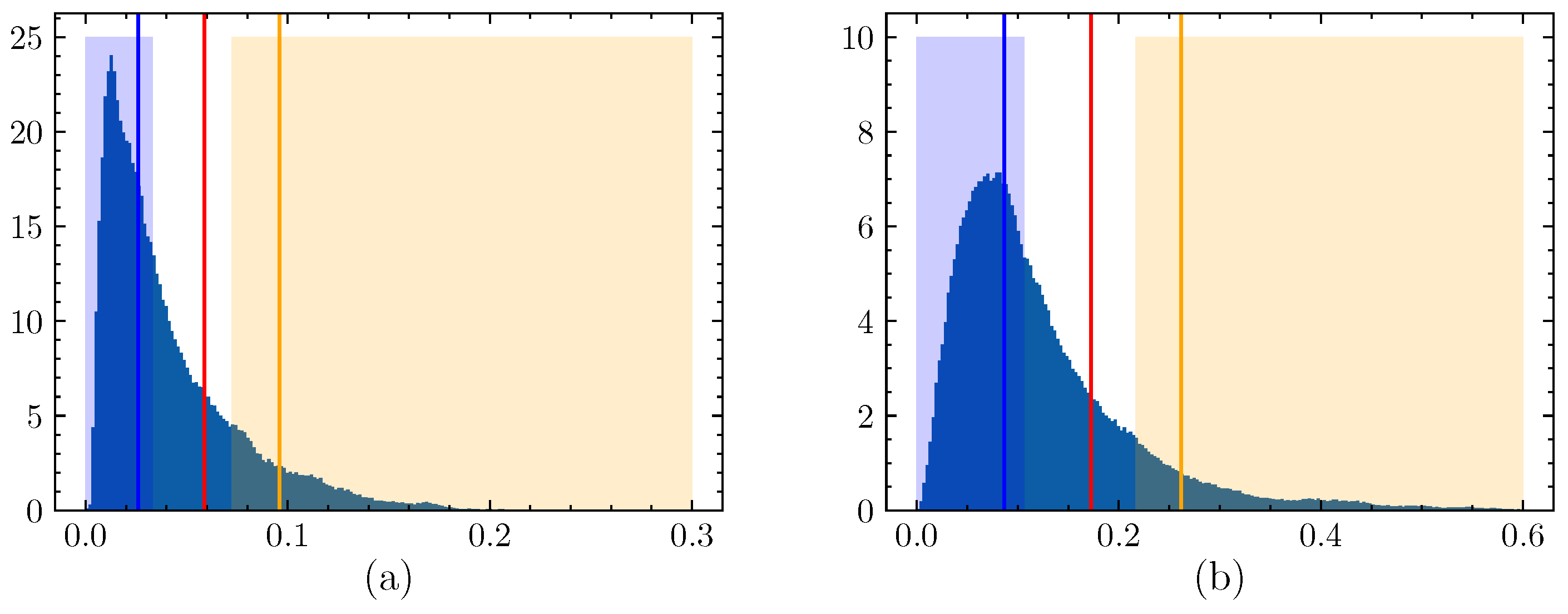
The traditional method uses the Otsu algorithm to automatically determine the threshold for generating the difference map. According to the guidance for generating the threshold, the ρ can easily be divided into two clusters, in which the part with a smaller value is used as the unchanged area data sample, and the part with a larger value is used as the changed area data sample. Using pseudo-label-based unsupervised learning methods can enable the network to mine the deep structural information of the data, reduce the interference of noisy samples, and generate better detection results.
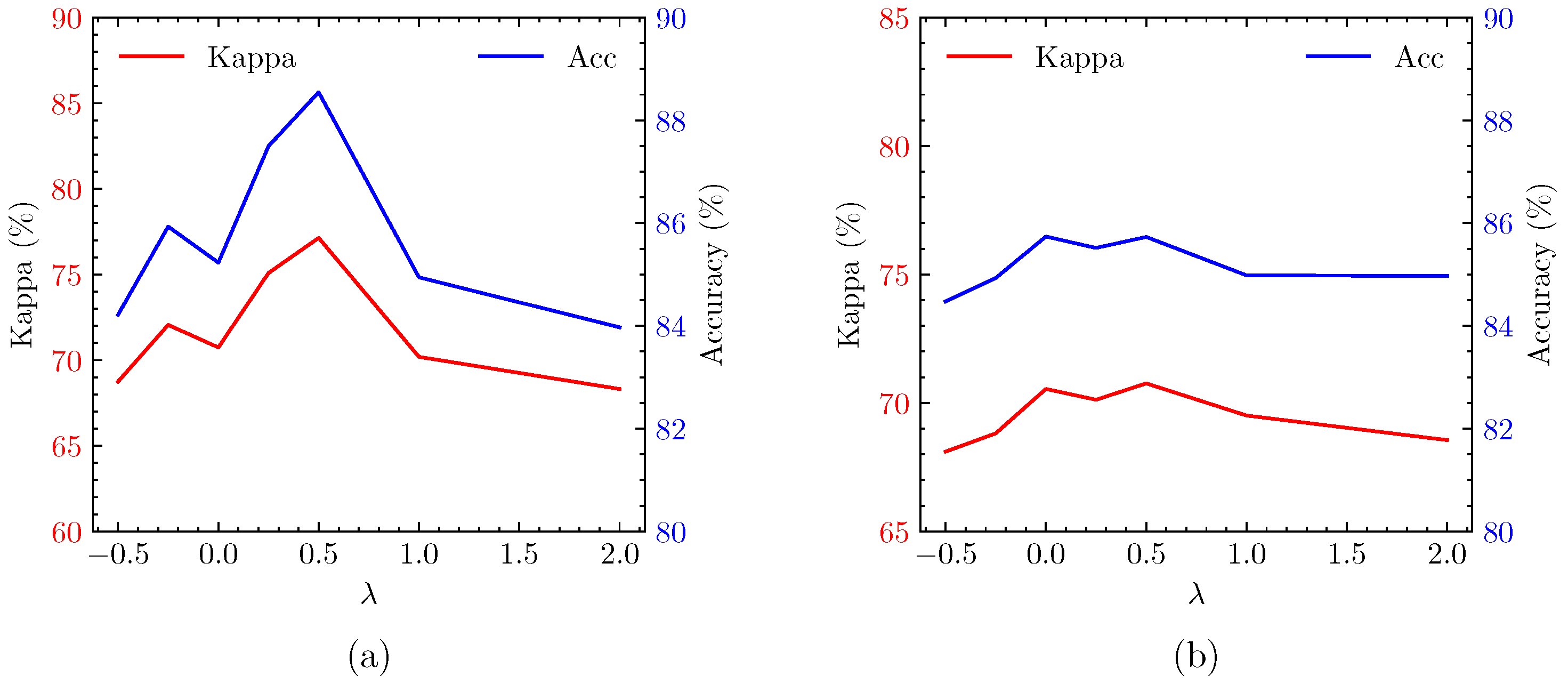
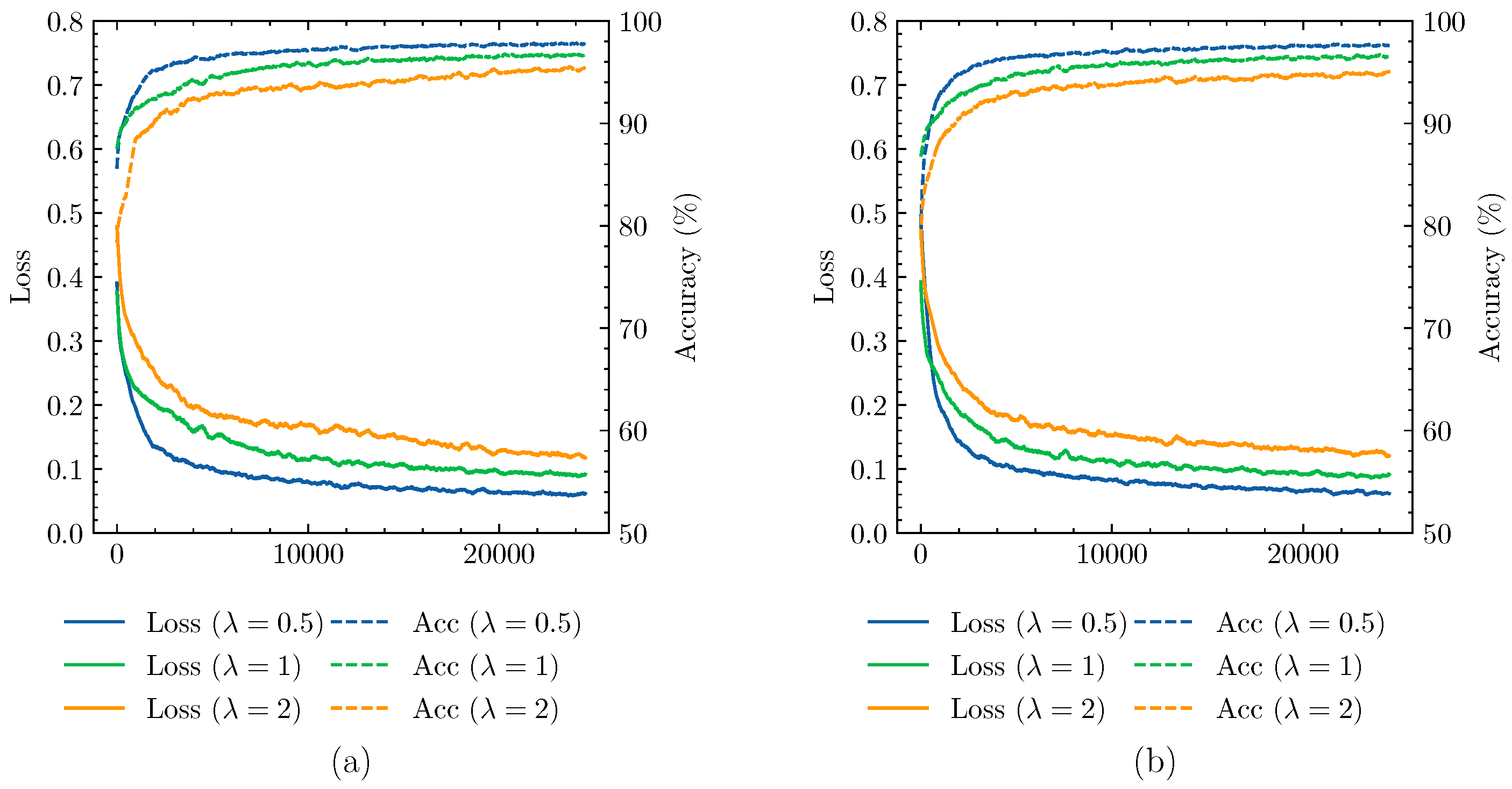
However, the critical samples generated by the hard threshold will reduce the sample quality, increase the proportion of false labels, and make the network difficult to optimize. In the subsequent experiments, if low-quality training samples are used, the network will exhibit poor convergence. The model’s detection accuracy is even worse than that of traditional methods. In this paper, we first calculate the distribution parameters of positive and negative samples, and set an overlap coefficient λ . The pseudo-labels’ generation formula is as follows:
Label Negative : ρ i , j < U mean + U std × λ , Ignore : others , Positive : C mean + C std × λ < ρ i , j ,
where the U mean , U std , C mean , and C std are the mean and variance of the negative and positive samples determined according to the hard threshold, respectively. Among them, when λ < 0 , we used the absolutely correct sample as the training sample, which can ensure the correctness of the sample, but reduces the diversity of the sample. When the λ > 0 , we gradually used more types of samples as training samples, but introduced a small number of wrong samples.

3.5. Network Overall Structure and Training Details

The overall structure of the network is shown in Table 1. The network structure is a module constructed based on the pipeline form, in which the input is the neighborhood at which the center point of the two image blocks is located, and the output is whether the region has changed and the probability of the prediction. The network can also easily be extended to multi-class changes.
We used a Linux workstation to complete the experiments. The computer has an NVIDIA RTX 3090 with 24G GPU memory, and we used pytorch to implement the code construction of the model. For the Hermiston dataset, we used 17 × 17 × 242 image pairs as input, while setting the λ to 0.1, and used all pseudo-labeled samples for network training. For the Bay and Santa Barbara datasets, we used 17 × 17 × 224 image pairs as the input, and set the λ to 0.5. As the image sizes of above two datasets were larger and the sample distribution was more uniform, among all the generated pseudo-label samples, we randomly sampled 64,000 positive samples and 64,000 negative samples as training sample sets. In training, all experiments used the same training parameters. Adam was used as the network optimizer, and the learning rate of the network was set to 0.0003. The batch size was set to 64, and the network was trained for 10 epochs before testing. In the test, for the Hermiston dataset, all pixels were used to calculate the final accuracy and kappa coefficient. For the Bay and Santa Barbara datasets, because the data contained an uncertain area mask, we only calculated the precision and kappa coefficients of pixels outside the mask area.

4. Result

To validate the effectiveness of the proposed methods, we conducted an experimental analysis on real hyperspectral change detection datasets. We selected several algorithms based on CVA methods and several based on deep learning methods as comparison algorithms. Finally, to demonstrate the effectiveness of the proposed feature extraction structure, we conducted ablation experiments to illustrate the advantages of our algorithm.

4.1. Datasets and Evaluation Criteria

The first dataset is the Hermiston dataset. As shown in Figure 2, the two hyperspectral images were acquired in 2004 and 2007 over the same area of Hermiston City Area, Oregon [46]. The co-registered images have the same size of 390 × 200 pixels, with the spatial resolution of 30 m and 242 available bands, as acquired by the Hyperion satellite. The reference image, shown in Figure 2, is a binary label representing whether the region undergoes meaningful changes.
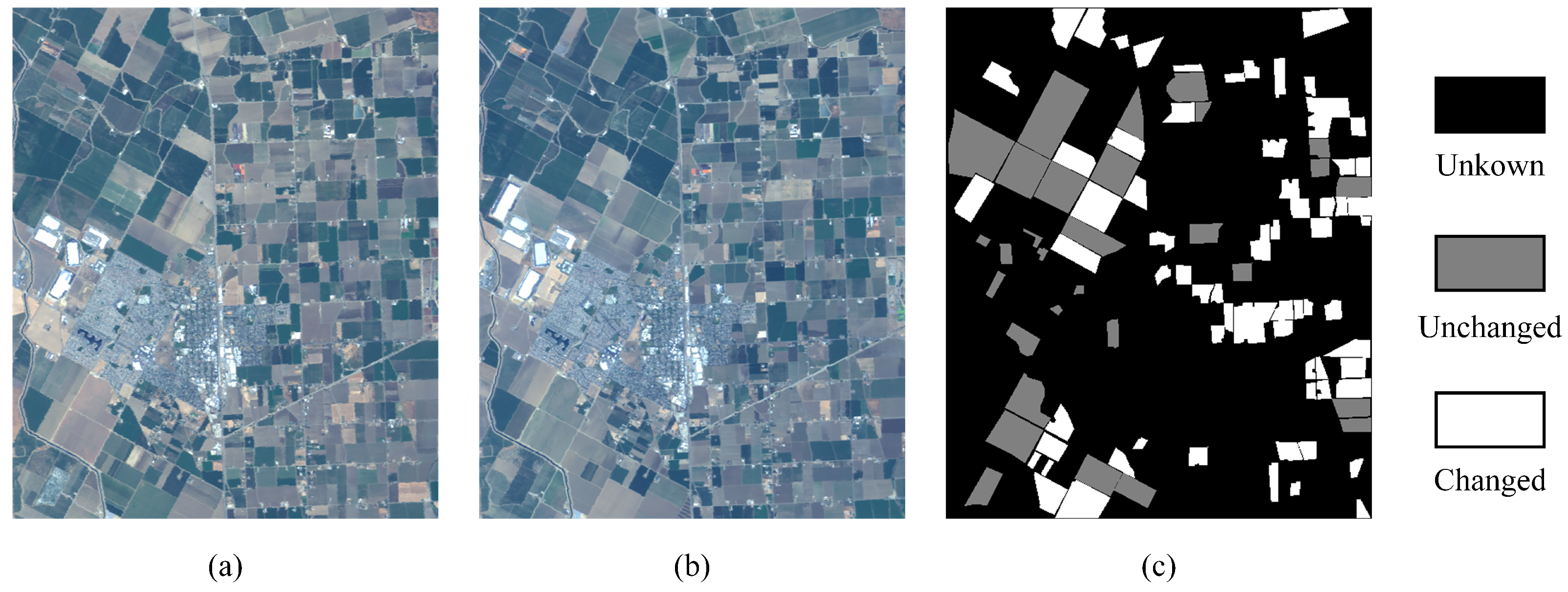
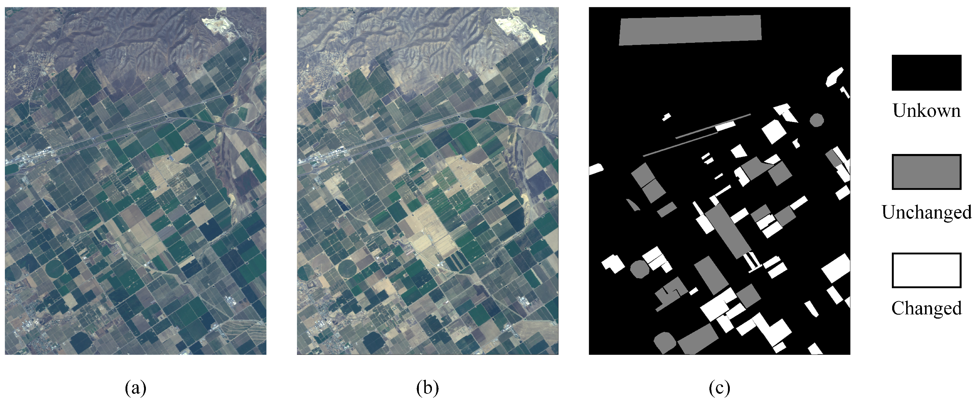
The other two datasets were the Bay Area dataset and the Santa Barbara dataset. These two datasets were collected from AVIRIS sensor with 224 spectral bands. As shown in Figure 3, the Bay Area dataset was captured above the Bay Area of Patterson, California, in 2013 and 2015, respectively. Both hyperspectral images and reference images have a spatial resolution of 984 × 740 . As shown in Figure 4, the Santa Barbara dataset was captured above the Santa Barbara, California in 2013 and 2014, respectively, and the image size was 600 × 500 . Differing from the previous dataset, these two datasets not only mark the changed and unchanged areas, but also mark the areas without accurate labels. Thus, the detection effect of different algorithms can be evaluated more accurately, and the influence of the noise area can be reduced.
To quantitatively evaluate the quality of the results of different algorithms, we use the overall accuracy ( O A ) and kappa coefficients ( K C ) to calculate the results of each algorithm. The O A is the proportion of correct samples to the total number of samples, which is calculated as follows:
O A = T P + T N T P + T N + F P + F N ,
where TP, TN, FP, and FN represent true positive, true negative, false positive, and false negative, respectively. The K C is based on the confusion matrix and is used to indicate the classification consistency with a large difference in the number of categories, which is calculated as follows:
P T P = ( T P + F P ) × ( T P + F N ) ,
P T N = ( T N + F P ) × ( T N + F N ) ,
P E = P T P + P T N ( T P + T N + F P + F N ) 2 ,
K C = O A P E 1 P E .

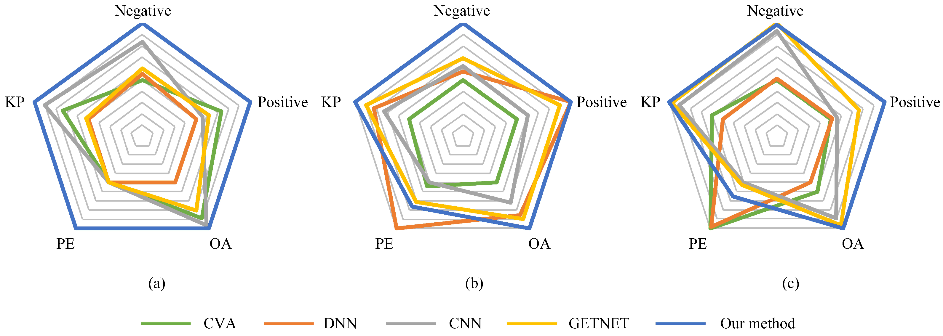
4.2. Comparison Results and Analysis

In this work, we compare the proposed algorithm with several representative change detection methods to demonstrate the effectiveness and generality of the proposed frameworks. Among them, CVA is a classical spectral-based change detection method that utilizes spectral difference maps to get the final result. DNN takes paired spectral vectors as input, and uses a multi-layer fully connected network to extract features and generate results. CNN utilizes patch images as input, and the convolutional neural network is used to extract features and then feed them to the classifier. GETNET uses the spectral vector to construct a two-dimensional correlation matrix, and uses CNN to reduce the parameters of the model.
Figure 5 shows the results of the compared and the proposed algorithms in Hermiston dataset, and the corresponding quantitative evaluation values are available in Table 2. As can be seen from Figure 5b, CVA can detect most of the change areas in the graph; however, due to the influence of the threshold selection, some areas where the change amplitude is at the critical value will lead to false detection, resulting in some small positive areas. As can be seen in table, the deep-learning-based methods consistently achieve better results than traditional methods. Although the DNN method achieves higher detection accuracy, it has more noise points than the CNN-based method, which need to be filtered out using additional pipelines. Compared with the GETNET method, the algorithm proposed in this paper achieves higher detection accuracy. At the same time, since GETNET makes predictions based on pixels, it will face the same problem as DNN, that is, there will be more noise in the results.
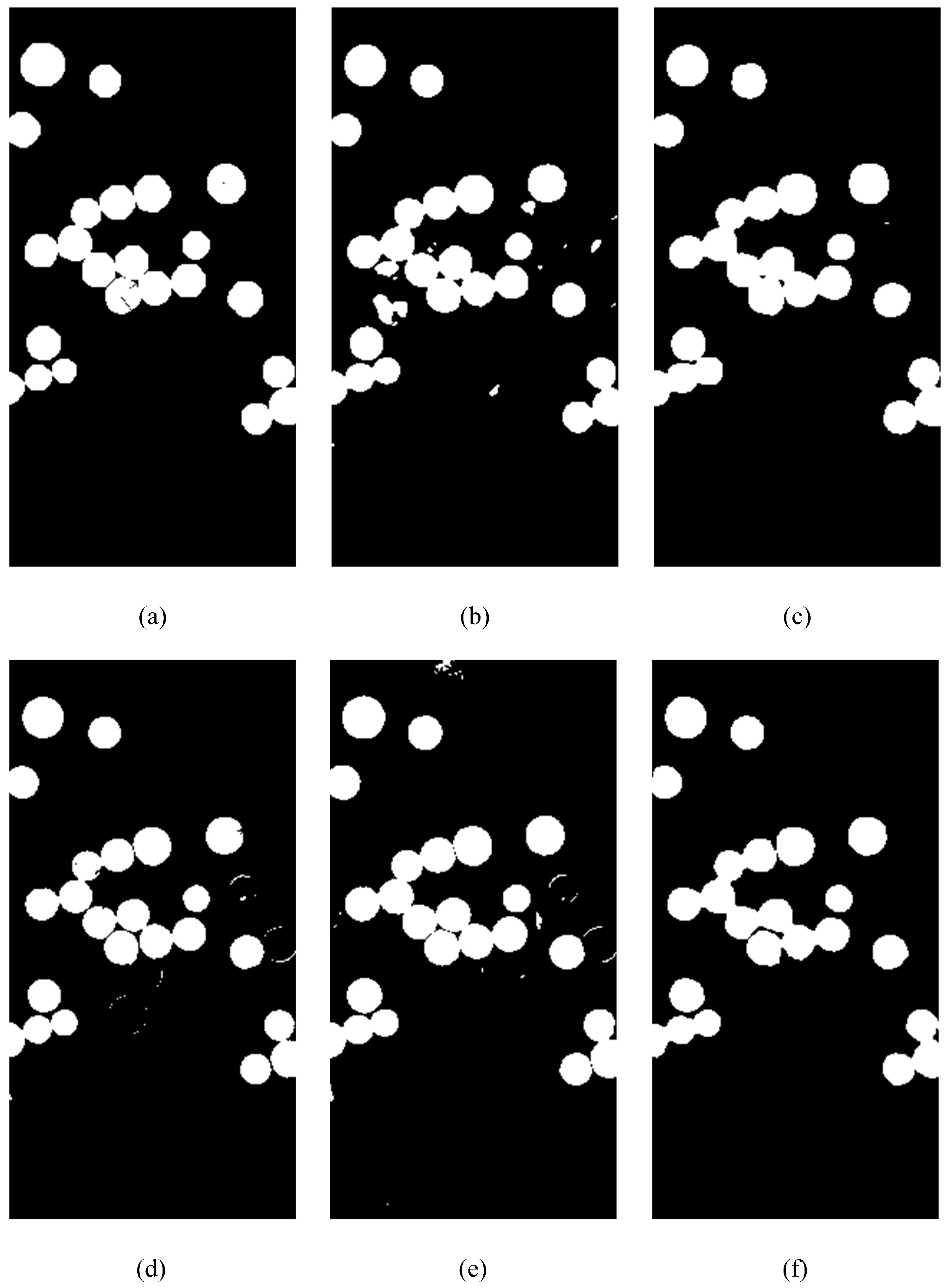
The test visualization results of the Bay Area dataset are shown in Figure 6, and the corresponding detection accuracy indicators are listed in Table 3. As can be seen from Figure 6b, the CVA method has a good performance in most positions in the graph. Although limited by the performance of the clustering method, this method inevitably has noise. It is worth noting that since the scene contains many confounding changes, the pixel-based method is more susceptible to noise, and the performance of the DNN and GETNET is even slightly lower than that in the traditional method. Although CNN methods can utilize more neighborhood information, the performance improvements compared to DNN are still limited. Compared with all other algorithms, the CD model proposed in this paper can better suppress noise and fully mine the depth information of pseudo-labels. The proposed method achieves better results in both qualitative and quantitative evaluations.
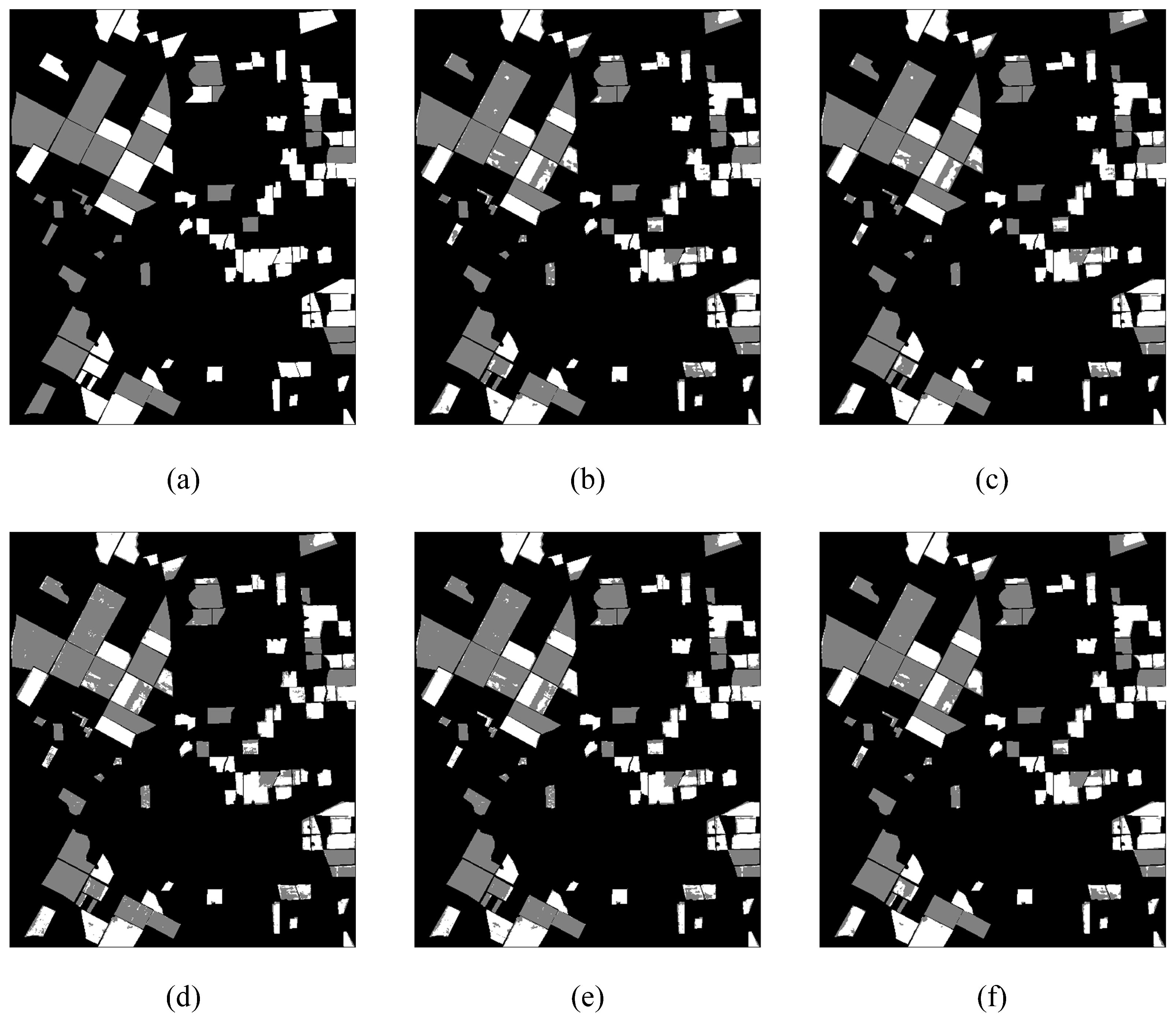
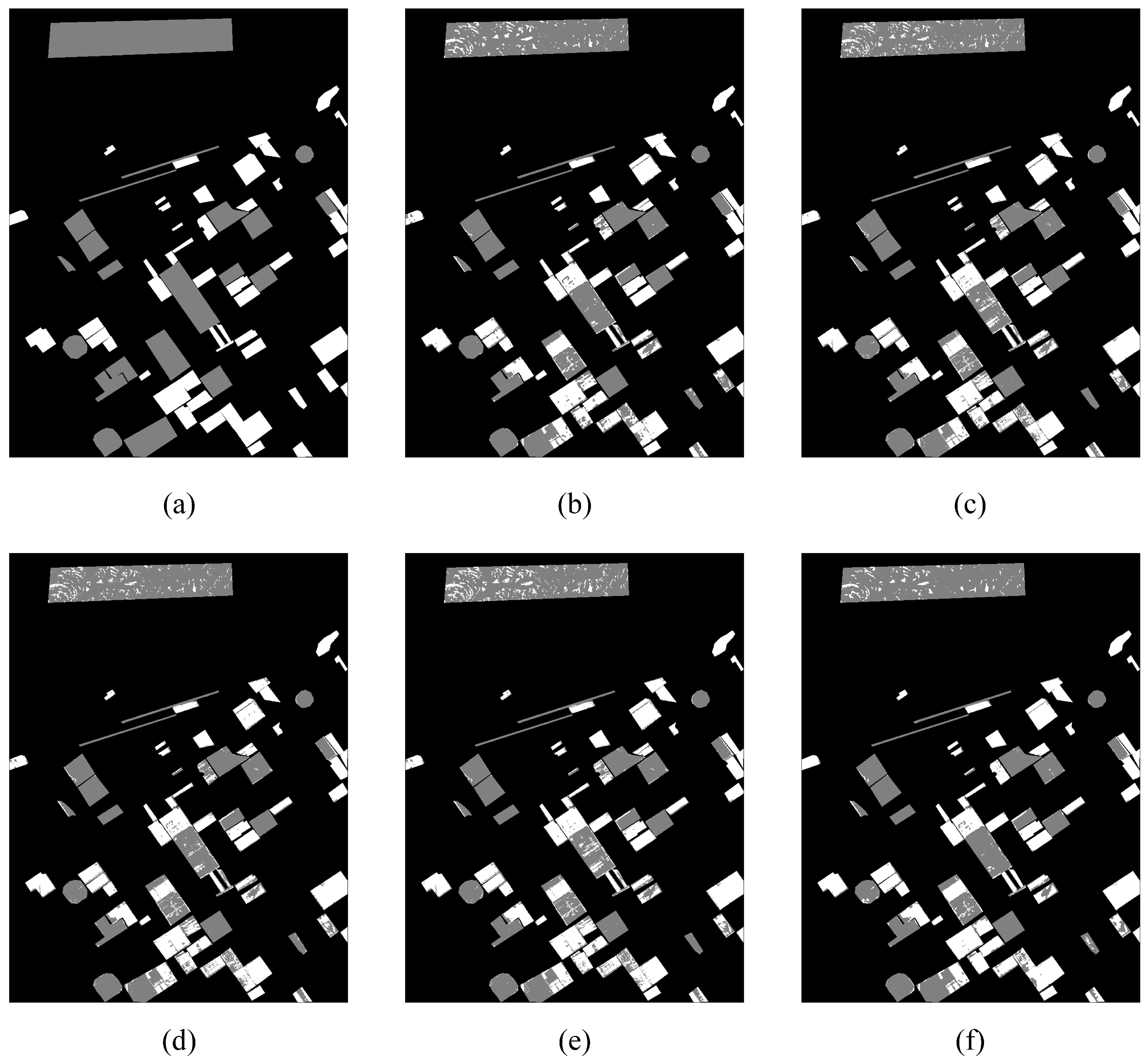
Similar to the experimental results on Bay Area data set, the Santa Barbara dataset achieves consistent performance gains on the test procedure. As shown in Figure 7 and Table 4, both GETNET and the method proposed in this paper have achieved encouraging detection results; however, due to the use of convolutional structure, the network proposed in this paper obtained slightly higher change detection accuracy. There was no change in a mountain area above the dataset; however, due to the influence of shadows and sensor noise, the results of different algorithms in this area are quite different. Likewise, CNN methods always outperform DNN methods due to their ability to integrate spatial information. Benefiting from the use of RNN to extract spectral information, the proposed method showed a a significant improvement in results compared with the CNN method.
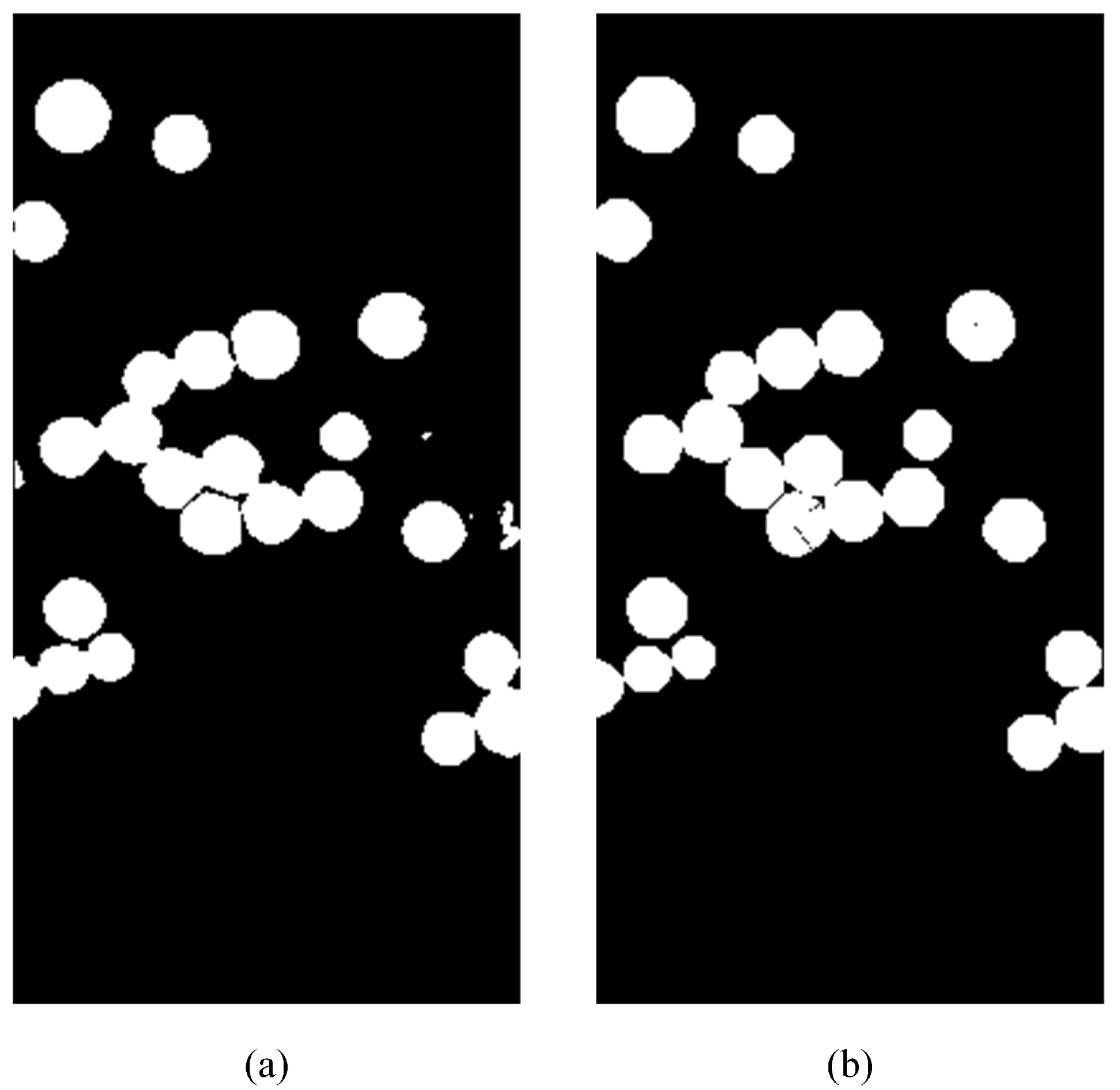
4.3. Ablation Study

To demonstrate that RNN can effectively extract spectral information from hyperspectral image data, we designed a contrastive network with the same structure as the network used in this paper, but without RNN. Table 2 shows that the network structure without RNN does not produce competitive results. Observing Figure 8, in the annular farmland area, using the RNN method can obtain a relatively more complete farmland area and, compared with the benchmark algorithm, the RNN method produces purer detection results in the boundary area between farmlands. The benchmark method can still produce relatively clean detection results, which also proves that the feature extraction structure of CNN can fully exploit the spatial information in hyperspectral images.
For hyperspectral image patch pairs with input dimensions 242 × 17 × 17 , Table 5 explains the effectiveness of the proposed structure from another perspective. The feature extraction network using RNN has fewer parameters and less computational complexity. Fewer parameters mean that the network is less prone to overfitting, which explains why better detection results and higher detection accuracy can be achieved with RNNs.

5. Discussion

5.1. Effectiveness of RNN on Spectra

To investigate the effectiveness of the RNN structure mentioned in the paper for the feature extraction of hyperspectral data, we construct an encoding–decoding structure using the feature-extraction module proposed in this paper, using the structure proposed in this paper as an encoder. The features of the hyperspectral data are extracted by the proposed module and, subsequently, a deconvolution is applied as a decoder to build an unsupervised end-to-end self-encoder. We extracted the feature layers behind the RNN in the generated feature map (the outputs of block 2 in Table 1), and we concatenated the feature values at corresponding positions in each layer as a pseudo-spectral sequence. The band of the generated spectral sequence is 32. To perform feature alignment, we used linear interpolation to upsample the extracted sequences. For comparison, we extracted the corresponding layer in the CNN structure for the analysis. We used Pearson correlation coefficients to analyze the input raw spectral sequences and the spectral sequences obtained by sampling in the corresponding feature maps. The experimental results are shown in Table 6. As expected, CNNs generate information that does not maintain the sequence characteristics of the original data due to their disordered connectivity over the spectral domain. Our proposed RNN structure does not explicitly constrain the regression mode of the model, but the generated information still has some correlation with the original data, proving that the proposed module helps to extract the spectral information from the input data.

5.2. Selection of Hyperparameters in Sample Generation

As shown in Figure 9, we show the histogram of the intensity distribution of the CD maps on the Bay Area dataset and the Santa Barbara dataset. The red line segment in the figure indicates the hard threshold value obtained using the threshold segmentation algorithm, where the part that is less than the threshold value is determined as the changed region (the region on the left of the red line segment) and the part greater than this threshold value is determined as the unchanged region (the region to the right of the red line segment). The blue line in the left region indicates the mean value of the unchanged region, and the orange line in the right region indicates the mean value of the changed region. The positive and negative samples selected using the sample selection strategy proposed in this paper are shown in the blue region and the orange region in the figure, respectively.
Since the neural network’s learning is affected by sample generation, for the pseudo-labels generated by unsupervised learning, in order to balance the selection of sample diversity and label feasibility, this part conducts sufficient experiments on the hyperparameter λ used in sample generation. In order to qualitatively evaluate the effect of different λ values, we trained the model with different sample sets. We conducted experiments on the Bay Area and Santa Barbara datasets. In this experiment, we set the number of positive and negative samples to 32,000, that is, a total of 64,000 training samples, and the other parameter settings remained unchanged.
The results are shown in Figure 10. Figure 10a,b, respectively, represent the detection results under different λ parameter settings, where the red line represents the KC of the model, and the green line represents the OA of the model. As can be seen from the figure, the performance of the network is directly related to the selected sample generation, and it is difficult to obtain a good model with a low-quality sample set. The left area in the figure represents selecting the correct samples as best as possible without considering the diversity, and the right area in the figure represents the selection of as many types of samples as possible, ignoring reliability. Setting the λ to 0.5 on the Bay Area dataset and the Santa Barbara dataset gives a good pseudo-labeled training sample set. This value is also consistent with our hypothesis, that is, the value of λ needs to balance the diversity of samples and the confidence rate of sample labels.
We also compared the curves of the training loss and accuracy of the network with lambda of 0.5, 1, and 2, respectively. As shown in Figure 11, for the λ parameter of 0.5 (the optimal parameter), the network converges to a better position at 10,000 iterations, which is faster compared to the other sample sets.

5.3. Compare the Performance of the Algorithm

The proposed method implements the two-class change detection task end-to-end in an unsupervised manner, and the above three experiments also demonstrate the adaptability and robustness of the proposed method. In Figure 12, we compare the performance of the five methods on five performance metrics, the correct rate of negative samples, the correct rate of positive samples, average precision, PE parameters and kappa coefficient, and each vertex represents the corresponding performance metric in the radar plot. As shown in Figure 12a, our method outperforms the other methods in all five performance metrics. Figure 12b,c also demonstrate that our method is more comprehensive in the five performance metrics.

5.4. Shortcomings of This Paper and Future Work

In this paper, we used RNN to mine the spectral information of input images and combined CNN to fuse the spatial information of hyperspectral data and complete the HSI-CD task. RNN has lower theoretical computational complexity floating point operations (FLOPs). Due to parallel implementation and code optimization, the actual running time of RNN on GPU is still not superior to that of CNN. Future work will focus on how to use more efficient feature extraction structures to mine both spectral and spatial information, as well as extend existing feature extraction structures to other tasks with hyperspectral data.

6. Conclusions

This paper proposes a hybrid CNN and RNN feature-extraction network for the hyperspectral change detection task. The network employs an RNN structure to extract spectral data while using the CNN structure to extract spatial information. Compared with other algorithms, the method proposed in this paper achieves better results in real HSI-CD datasets. Simultaneously, we perform ablation experiments on the proposed structure, which proves that the proposed structure has a more vital representation ability for spectral information. Extensive experiments incorporating both qualitative and quantitative evaluations demonstrate that our method produces consistent and substantial gains.

Author Contributions

Conceptualization and methodology, H.Z.; software, H.Z. and K.F.; resources, Y.W. and M.G.; writing—original draft preparation, H.Z.; writing—review and editing, H.Z. and K.F. All authors have read and agreed to the published version of the manuscript.

Funding

This research was funded by Key-Area Research and Development Program of Guangdong Province grant number 2020B090921001.

Conflicts of Interest

The authors declare no conflict of interest.

References

  1. Cheng, G.; Yao, Y.; Li, S.; Li, K.; Xie, X.; Wang, J.; Yao, X.; Han, J. Dual-aligned oriented detector. IEEE Trans. Geosci. Remote Sens. 2022, 60, 5618111. [Google Scholar] [CrossRef]
  2. Liu, J.; Gong, M.; Qin, K.; Zhang, P. A deep convolutional coupling network for change detection based on heterogeneous optical and radar images. IEEE Trans. Neural Netw. Learn. Syst. 2016, 29, 545–559. [Google Scholar] [CrossRef]
  3. Zhang, P.; Gong, M.; Su, L.; Liu, J.; Li, Z. Change detection based on deep feature representation and mapping transformation for multi-spatial-resolution remote sensing images. ISPRS J. Photogramm. Remote Sens. 2016, 116, 24–41. [Google Scholar] [CrossRef]
  4. Gong, M.; Zhan, T.; Zhang, P.; Miao, Q. Superpixel-based difference representation learning for change detection in multispectral remote sensing images. IEEE Trans. Geosci. Remote Sens. 2017, 55, 2658–2673. [Google Scholar] [CrossRef]
  5. Zhang, H.; Gong, M.; Zhang, P.; Su, L.; Shi, J. Feature-level change detection using deep representation and feature change analysis for multispectral imagery. IEEE Geosci. Remote Sens. Lett. 2016, 13, 1666–1670. [Google Scholar] [CrossRef]
  6. Wu, Y.; Mu, G.; Qin, C.; Miao, Q.; Ma, W.; Zhang, X. Semi-supervised hyperspectral image classification via spatial-regulated self-training. Remote Sens. 2020, 12, 159. [Google Scholar] [CrossRef]
  7. Wu, Y.; Li, J.; Yuan, Y.; Qin, A.K.; Miao, Q.; Gong, M. Commonality autoencoder: Learning common features for change detection from heterogeneous images. IEEE Trans. Neural Netw. Learn. Syst. 2021, 33, 4257–4270. [Google Scholar] [CrossRef]
  8. Cheng, G.; Wang, G.; Han, J. ISNet: Towards Improving Separability for Remote Sensing Image Change Detection. IEEE Trans. Geosci. Remote Sens. 2022, 60, 5623811. [Google Scholar] [CrossRef]
  9. Liu, J.; Gong, M.; Miao, Q.; Su, L.; Li, H. Change detection in synthetic aperture radar images based on unsupervised artificial immune systems. Appl. Soft Comput. 2015, 34, 151–163. [Google Scholar] [CrossRef]
  10. Zhao, Q.; Ma, J.; Gong, M.; Li, H.; Zhan, T. Three-class change detection in synthetic aperture radar images based on deep belief network. J. Comput. Theor. Nanosci. 2016, 13, 3757–3762. [Google Scholar] [CrossRef]
  11. Ma, W.; Wu, Y.; Gong, M.; Xiong, Y.; Yang, H.; Hu, T. Change detection in SAR images based on matrix factorisation and a Bayes classifier. Int. J. Remote Sens. 2019, 40, 1066–1091. [Google Scholar] [CrossRef]
  12. Wang, Q.; Yuan, Z.; Du, Q.; Li, X. GETNET: A general end-to-end 2-D CNN framework for hyperspectral image change detection. IEEE Trans. Geosci. Remote Sens. 2018, 57, 3–13. [Google Scholar] [CrossRef]
  13. Deng, J.; Wang, K.; Deng, Y.; Qi, G. PCA-based land-use change detection and analysis using multitemporal and multisensor satellite data. Int. J. Remote Sens. 2008, 29, 4823–4838. [Google Scholar] [CrossRef]
  14. Bovolo, F.; Marchesi, S.; Bruzzone, L. A framework for automatic and unsupervised detection of multiple changes in multitemporal images. IEEE Trans. Geosci. Remote Sens. 2011, 50, 2196–2212. [Google Scholar] [CrossRef]
  15. Liu, S.; Bruzzone, L.; Bovolo, F.; Zanetti, M.; Du, P. Sequential spectral change vector analysis for iteratively discovering and detecting multiple changes in hyperspectral images. IEEE Trans. Geosci. Remote Sens. 2015, 53, 4363–4378. [Google Scholar] [CrossRef]
  16. Thonfeld, F.; Feilhauer, H.; Braun, M.; Menz, G. Robust Change Vector Analysis (RCVA) for multi-sensor very high resolution optical satellite data. Int. J. Appl. Earth Obs. Geoinf. 2016, 50, 131–140. [Google Scholar] [CrossRef]
  17. Malila, W. Change vector analysis: An approach for detecting forest changes with Landsat. In Proceedings of the Machine Processing of Remotely Sensed Data Symposium, Purdue University, West Lafayette, IN, USA, 3–6 June 1980; pp. 326–335. [Google Scholar]
  18. Bruzzone, L.; Prieto, D.F. Automatic analysis of the difference image for unsupervised change detection. IEEE Trans. Geosci. Remote Sens. 2000, 38, 1171–1182. [Google Scholar] [CrossRef]
  19. Bovolo, F.; Bruzzone, L. A theoretical framework for unsupervised change detection based on change vector analysis in the polar domain. IEEE Trans. Geosci. Remote Sens. 2006, 45, 218–236. [Google Scholar] [CrossRef]
  20. Saha, S.; Bovolo, F.; Bruzzone, L. Unsupervised deep change vector analysis for multiple-change detection in VHR images. IEEE Trans. Geosci. Remote Sens. 2019, 57, 3677–3693. [Google Scholar] [CrossRef]
  21. Nielsen, A.A.; Conradsen, K.; Simpson, J.J. Multivariate alteration detection (MAD) and MAF postprocessing in multispectral, bitemporal image data: New approaches to change detection studies. Remote Sens. Environ. 1998, 64, 1–19. [Google Scholar] [CrossRef] [Green Version]
  22. Gong, M.; Zhou, Z.; Ma, J. Change detection in synthetic aperture radar images based on image fusion and fuzzy clustering. IEEE Trans. Image Process. 2011, 21, 2141–2151. [Google Scholar] [CrossRef] [PubMed]
  23. Celik, T. Unsupervised change detection in satellite images using principal component analysis and k-means clustering. IEEE Geosci. Remote Sens. Lett. 2009, 6, 772–776. [Google Scholar] [CrossRef]
  24. Nielsen, A.A. The regularized iteratively reweighted MAD method for change detection in multi-and hyperspectral data. IEEE Trans. Image Process. 2007, 16, 463–478. [Google Scholar] [CrossRef] [PubMed]
  25. Tang, P.; Yang, J.; Zhang, C.; Zhu, D.; Su, W. An object-oriented post-classification remote sensing change detection after the pixel ratio. Remote Sens. Inf. 2010, 1, 69–72. [Google Scholar]
  26. Al Rawashdeh, S.B. Evaluation of the differencing pixel-by-pixel change detection method in mapping irrigated areas in dry zones. Int. J. Remote Sens. 2011, 32, 2173–2184. [Google Scholar] [CrossRef]
  27. Liu, S.; Bruzzone, L.; Bovolo, F.; Du, P. Unsupervised multitemporal spectral unmixing for detecting multiple changes in hyperspectral images. IEEE Trans. Geosci. Remote Sens. 2016, 54, 2733–2748. [Google Scholar] [CrossRef]
  28. Hsieh, C.C.; Hsieh, P.F.; Lin, C.W. Subpixel change detection based on abundance and slope features. In Proceedings of the 2006 IEEE International Symposium on Geoscience and Remote Sensing, Denver, CO, USA, 31 July–4 August 2006; pp. 775–778. [Google Scholar]
  29. Ertürk, A.; Iordache, M.D.; Plaza, A. Sparse unmixing with dictionary pruning for hyperspectral change detection. IEEE J. Sel. Top. Appl. Earth Obs. Remote Sens. 2016, 10, 321–330. [Google Scholar] [CrossRef]
  30. Ertürk, A.; Iordache, M.D.; Plaza, A. Sparse unmixing-based change detection for multitemporal hyperspectral images. IEEE J. Sel. Top. Appl. Earth Obs. Remote Sens. 2015, 9, 708–719. [Google Scholar] [CrossRef]
  31. Li, H.; Wu, K.; Xu, Y. An Integrated Change Detection Method Based on Spectral Unmixing and the CNN for Hyperspectral Imagery. Remote Sens. 2022, 14, 2523. [Google Scholar] [CrossRef]
  32. Qu, Y.; Wang, W.; Guo, R.; Ayhan, B.; Kwan, C.; Vance, S.; Qi, H. Hyperspectral anomaly detection through spectral unmixing and dictionary-based low-rank decomposition. IEEE Trans. Geosci. Remote Sens. 2018, 56, 4391–4405. [Google Scholar] [CrossRef]
  33. Seydi, S.T.; Hasanlou, M. A new structure for binary and multiple hyperspectral change detection based on spectral unmixing and convolutional neural network. Measurement 2021, 186, 110137. [Google Scholar] [CrossRef]
  34. Seydi, S.T.; Shah-Hosseini, R.; Hasanlou, M. New framework for hyperspectral change detection based on multi-level spectral unmixing. Appl. Geomat. 2021, 13, 763–780. [Google Scholar] [CrossRef]
  35. Huang, F.; Yu, Y.; Feng, T. Hyperspectral remote sensing image change detection based on tensor and deep learning. J. Vis. Commun. Image Represent. 2019, 58, 233–244. [Google Scholar] [CrossRef]
  36. Zhan, Y.; Fu, K.; Yan, M.; Sun, X.; Wang, H.; Qiu, X. Change detection based on deep siamese convolutional network for optical aerial images. IEEE Geosci. Remote Sens. Lett. 2017, 14, 1845–1849. [Google Scholar] [CrossRef]
  37. Mou, L.; Bruzzone, L.; Zhu, X.X. Learning spectral-spatial-temporal features via a recurrent convolutional neural network for change detection in multispectral imagery. IEEE Trans. Geosci. Remote Sens. 2018, 57, 924–935. [Google Scholar] [CrossRef]
  38. Ken, S.; Akayuki, O. Change Detection from a Street Image Pair Using CNN Features and Superpixel Segmentation. 2015. Available online: http://www.ucl.nuee.nagoya-u.ac.jp/~sakurada/document/71-Sakurada-BMVC15.pdf (accessed on 1 September 2022).
  39. Wang, Q.; Zhang, X.; Chen, G.; Dai, F.; Gong, Y.; Zhu, K. Change detection based on Faster R-CNN for high-resolution remote sensing images. Remote Sens. Lett. 2018, 9, 923–932. [Google Scholar] [CrossRef]
  40. Li, X.; Yuan, Z.; Wang, Q. Unsupervised deep noise modeling for hyperspectral image change detection. Remote Sens. 2019, 11, 258. [Google Scholar] [CrossRef]
  41. Li, L.; Yang, Z.; Jiao, L.; Liu, F.; Liu, X. High-resolution SAR change detection based on ROI and SPP net. IEEE Access 2019, 7, 177009–177022. [Google Scholar] [CrossRef]
  42. Gao, F.; Wang, X.; Gao, Y.; Dong, J.; Wang, S. Sea ice change detection in SAR images based on convolutional-wavelet neural networks. IEEE Geosci. Remote Sens. Lett. 2019, 16, 1240–1244. [Google Scholar] [CrossRef]
  43. Zhang, X.; Su, H.; Zhang, C.; Atkinson, P.M.; Tan, X.; Zeng, X.; Jian, X. A Robust Imbalanced SAR Image Change Detection Approach Based on Deep Difference Image and PCANet. arXiv 2020, arXiv:2003.01768. [Google Scholar]
  44. Liu, J.; Chen, K.; Xu, G.; Sun, X.; Yan, M.; Diao, W.; Han, H. Convolutional neural network-based transfer learning for optical aerial images change detection. IEEE Geosci. Remote Sens. Lett. 2019, 17, 127–131. [Google Scholar] [CrossRef]
  45. Zhou, Y.; Li, X. Unsupervised Self-training Algorithm Based on Deep Learning for Optical Aerial Images Change Detection. arXiv 2020, arXiv:2010.07469. [Google Scholar]
  46. López-Fandiño, J.; Garea, A.S.; Heras, D.B.; Argüello, F. Stacked autoencoders for multiclass change detection in hyperspectral images. In Proceedings of the IGARSS 2018—2018 IEEE International Geoscience and Remote Sensing Symposium, Valencia, Spain, 22–27 July 2018; pp. 1906–1909. [Google Scholar]
Figure 1. Architecture of our proposed method, which contains three main parts: the convolutional neural network part, recurrent neural network part and the final, fully connected layer part.
Remotesensing 14 04646 g001
Figure 2. The Hermiston City area dataset. (a) Image acquired in 2004. (b) Image acquired in 2007. (c) Reference map.
Remotesensing 14 04646 g002
Figure 3. The Bay Area dataset. (a) Image acquired in 2013. (b) Image acquired in 2015. (c) Reference map.
Remotesensing 14 04646 g003
Figure 4. The Santa Barbara dataset. (a) Image acquired in 2013. (b) Image acquired in 2014. (c) Reference map.
Remotesensing 14 04646 g004
Figure 5. Comparison results of different algorithms on the Hermiston City Area dataset. (a) Reference map. (b) CVA. (c) DNN. (d) CNN. (e) GETNET. (f) Our method.
Remotesensing 14 04646 g005
Figure 6. Comparison results of different algorithms on the Bay Area dataset. (a) Reference map. (b) CVA. (c) DNN. (d) CNN. (e) GETNET. (f) Our method.
Remotesensing 14 04646 g006
Figure 7. Comparison results of different algorithms on the Santa Barbara dataset. (a) Reference map. (b) CVA. (c) DNN. (d) CNN. (e) GETNET. (f) Our method.
Remotesensing 14 04646 g007
Figure 8. Visualization of detection results with and without RNN. (a) Without RNN. (b) With RNN.
Remotesensing 14 04646 g008
Figure 9. The Sample Distribution on the Bay Area dataset and the Santa Barbara dataset. (a) The Bay Area dataset. (b) The Santa Barbara dataset.
Remotesensing 14 04646 g009
Figure 10. The influence of parameter λ on the Bay Area dataset and the Santa Barbara dataset. (a) The influence of λ on the Bay Area dataset. (b) The influence of λ on the Santa Barbara dataset.
Remotesensing 14 04646 g010
Figure 11. The network training accuracy and loss curves for the Bay Area and Santa Barbara datasets. (a) The Bay Area dataset. (b) The Santa Barbara dataset.
Remotesensing 14 04646 g011
Figure 12. Metrics comparison of different algorithms on the three datasets. (a) Metrics comparison of the Hermiston City Area dataset. (b) Metrics comparison on the Bay Area dataset. (c) Metrics comparison of the Santa Barbara dataset.
Remotesensing 14 04646 g012
Table 1. The overall structure of the network.
StageModuleParameter
Block1Convchannel = 128
size = 1
ReLU
Convchannel = 128
stride = 2
size = 3
ReLU
Block2RNNchannel = 32
Tanh
Convchannel = 32
stride = 2
size = 3
ReLU
Block3RNNchannel = 8
Tanh
Convchannel = 8
stride = 2
size = 3
ReLU
Flatten
HeadLinearchannel = 32
ReLU
Linearchannel = 8
ReLU
Linearchannel = 2
Table 2. Quantitative evaluation of experimental results of different methods on Hermiston City Area dataset.
AlgorithmNegativePositiveOAPEKC
CVA0.990.9097.9477.3090.93
DNN0.990.9698.4078.2092.68
CNN0.990.9198.2277.2292.20
GETNET0.990.9498.4577.6393.08
Ours (without RNN)0.990.9498.3777.6692.70
Ours (with RNN)0.990.9598.5877.7393.63
Table 3. Quantitative evaluation of experimental results of different methods on Bay Area data set.
AlgorithmNegativePositiveOAPEKC
CVA0.780.9585.3749.5571.00
DNN0.780.9482.7349.5469.73
CNN0.790.9485.8449.6071.91
GETNET0.780.9484.8049.5769.85
Ours0.790.9586.0859.5572.41
Table 4. Quantitative evaluation of experimental results of different methods on Santa Barbara dataset.
AlgorithmNegativePositiveOAPEKC
CVA0.880.7984.7451.9668.23
DNN0.880.7984.0651.9466.83
CNN0.920.7986.5951.2872.47
GETNET0.930.8087.0351.2473.39
Ours0.920.8187.2551.4673.72
Table 5. Comparison of network parameters and flops.
Network StructureParametersFLOPs
Without RNN0.221M43.679M
With RNN0.192M42.277M
Table 6. Pearson correlation coefficients of CNN-based feature extractor and RNN-based feature extractor.
MethodPearson Correlation Coefficients
CNN-based−0.398
RNN-based0.275
Publisher’s Note: MDPI stays neutral with regard to jurisdictional claims in published maps and institutional affiliations.

