
Spectral Indices as a Tool to Assess the Moisture Status of Forest Habitats
 , ,
, ,
Abstract
:1. Introduction
2. Materials and Methods
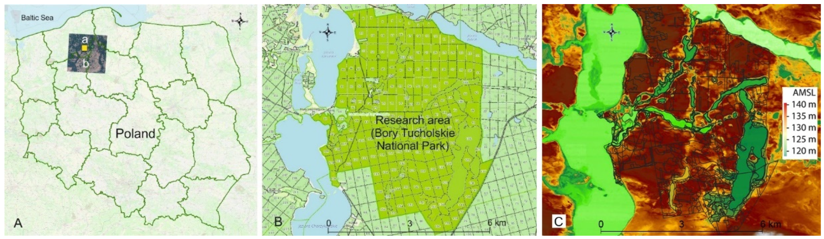
2.1. Research Area
2.2. Satellite Data
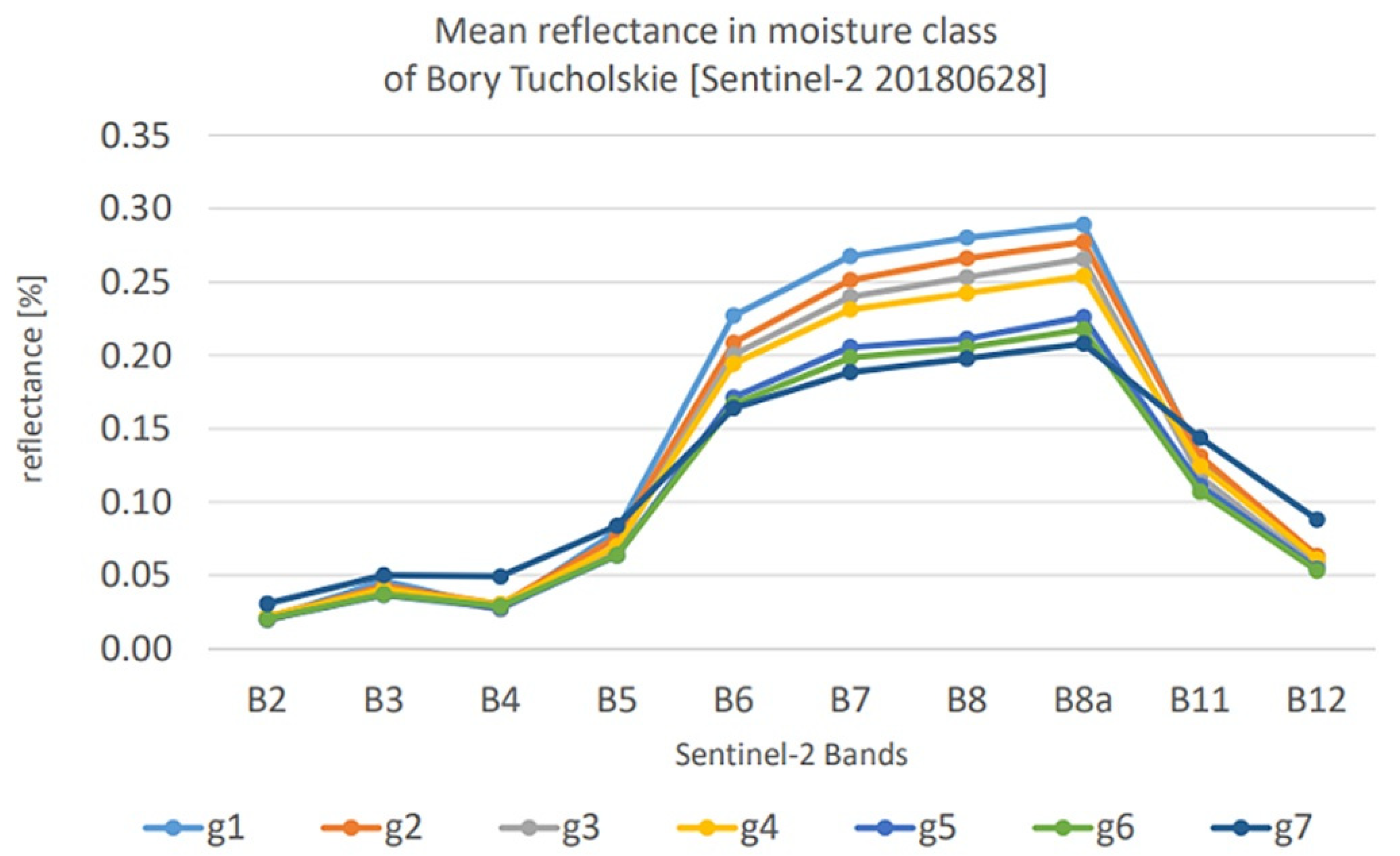
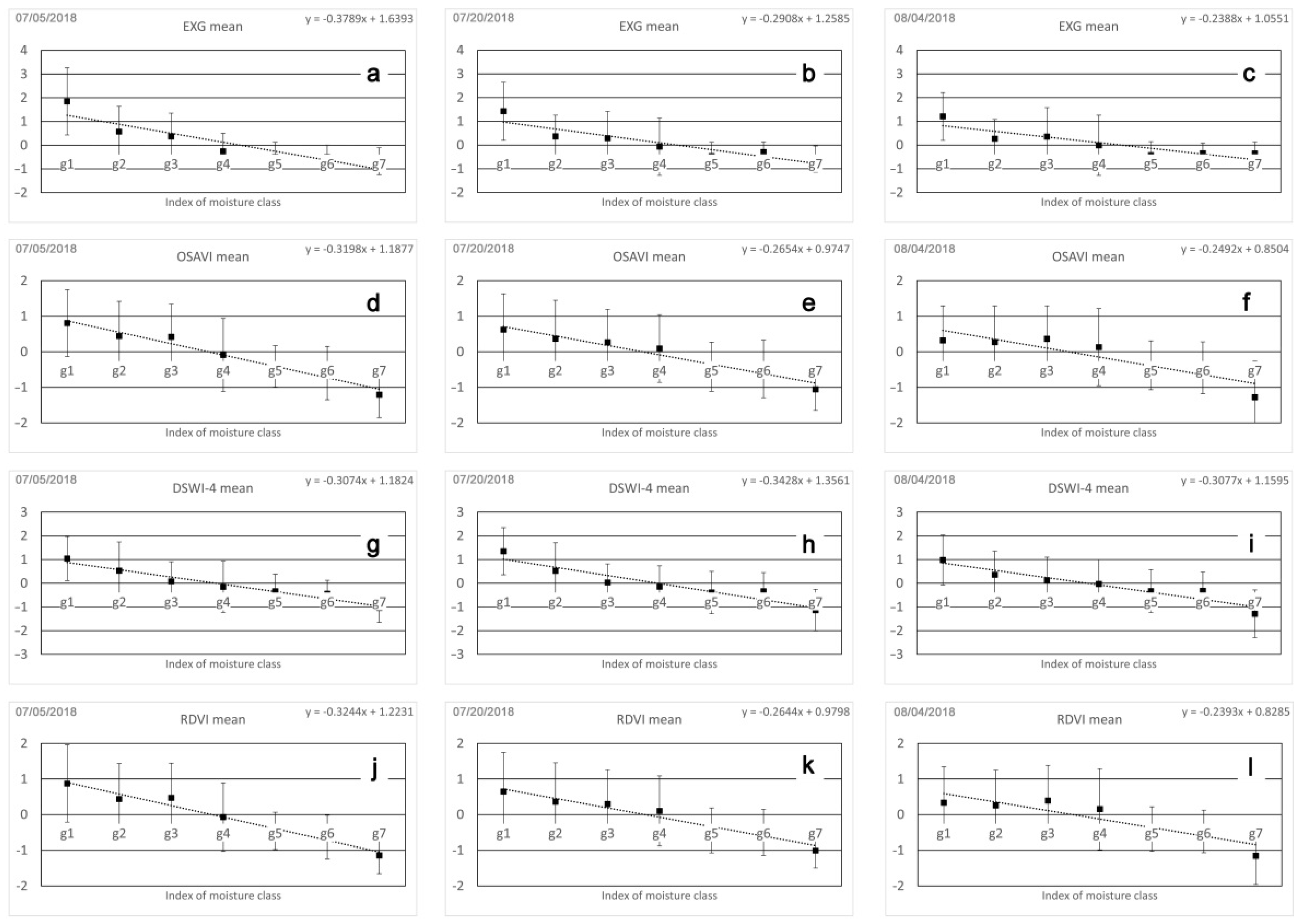
3. Results
4. Discussion
5. Conclusions
6. Patents
Supplementary Materials
Author Contributions
Funding
Data Availability Statement
Acknowledgments
Conflicts of Interest
References
- Ellison, D. Forests and Water. Background Analytical Study, 2; United Nations Forum on Forests: New York, NY, USA, 2018. [Google Scholar]
- Ellison, D.; Morris, C.E.; Locatelli, B.; Sheil, D.; Cohen, J.; Murdiyarso, D.; Gutierrez, V.; Van Noordwijk, M.; Creed, I.F.; Pokorny, J.; et al. Trees, forests and water: Cool insights for a hot world. Glob. Environ. Chang. 2017, 43, 51–61. [Google Scholar] [CrossRef]
- Savill, P.S. Land classifcation for plantation forestry. Ir. For. 1983, 40, 78–91. [Google Scholar]
- Farrelly, N.; Fealy, R.M.; Radford, T. The use of site factors and site classification methods for the assessment of site quality and forest productivity in Ireland. Ir. For. 2009, 66, 21–38. [Google Scholar]
- Gauer, J.; Feger, K.-H.; Schwärzel, K. Erfassung und Bewertung des Wasserhaushalts von Waldstandorten in der forstlichen Standortskartierung: Gegenwärtiger Stand und künftige Anforderungen. Wald. Landsch. Nat. 2011, 12, 7–16. [Google Scholar]
- Zielony, R.; Bańkowski, J.; Cieśla, A.; Czerepko, J.; Czępińska-Kamińska, D.; Kliczkowska, A.; Kowalkowski, A.; Krzyżanowski, A.; Mąkosa, K.; Sikorska, E. Siedliskowe Podstawy Hodowli Lasu. Załącznik do Zasad Hodowli Lasu. (Habitat Basics of Silviculture. Annex to the Principles of Silviculture); CILP: Warszawa, Poland, 2004; pp. 1–264. (In Polish) [Google Scholar]
- Święcicki, Z. (Ed.) Instrukcja Urządzania Lasu, Część 2: Instrukcja Wyróżniania i Kartowania w Lasach Państwowych Typów Siedliskowych Lasu oraz Zbiorowisk Roślinnych. (Instruction of Forest Management, Part 2: Instruction for Distinguishing and Mapping Forest Habitat Types and Plant Communities in the State Forests); CILP: Warszawa, Poland, 2012. (In Polish) [Google Scholar]
- Zajączkowski, G.; Jabłoński, M.; Jabłoński, T.; Szmidla, H.; Kowalska, A.; Małachowska, J.; Piwnicki, J. Raport o Stanie Lasów w Polsce (Report on the State of Forests in Poland); CILP: Warszawa, Poland, 2020. (In Polish) [Google Scholar]
- Albergel, C.; De Rosnay, P.; Gruhier, C.; Munoz-Sabater, J.; Hasenauer, S.; Isaksen, L.; Kerr, Y.; Wagner, W. Evaluation of remotely sensed and modelled soil moisture products using global ground-based in situ observations. Remote Sens. Environ. 2012, 118, 215–226. [Google Scholar] [CrossRef]
- Kędzior, M.; Zawadzki, J. Comparative study of soil moisture estimations from SMOS satellite mission, GLDAS database, and cosmic-ray neutrons measurements at COSMOS station in eastern Poland. Geoderma 2016, 283, 21–31. [Google Scholar] [CrossRef]
- Babaeian, E.; Sadeghi, M.; Jones, S.B.; Montzka, C.; Vereecken, H.; Tuller, M. Ground, proximal, and satellite remote sensing of soil moisture. Rev. Geophys. 2019, 57, 530–616. [Google Scholar] [CrossRef]
- Sabaghy, S.; Walker, J.P.; Renzullo, L.J.; Akbar, R.; Chan, S.; Chaubell, J.; Das, N.; Dunbar, R.S.; Entekhabi, D.; Gevaert, A. Comprehensive analysis of alternative downscaled soil moisture products. Remote Sens. Environ. 2020, 239, 111586. [Google Scholar] [CrossRef]
- Polcher, J.; Piles, M.; Gelati, E.; Barella-Ortiz, A.; Tello, M. Comparing surface-soil moisture from the SMOS mission and the ORCHIDEE land-surface model over the Iberian Peninsula. Remote Sens. Environ. 2016, 174, 69–81. [Google Scholar] [CrossRef]
- Pinnington, E.; Amezcua, J.; Cooper, E.; Dadson, S.; Ellis, R.; Peng, J.; Robinson, E.; Quaife, T. Improving soil moisture prediction of a high–resolution land surface model by parameterising pedotransfer functions through assimilation of SMAP satellite data. Hydrol. Earth Syst. Sci. 2021, 25, 1617–1641. [Google Scholar] [CrossRef]
- Shellito, P.J.; Kumar, S.V.; Santanello, J.A.; Lawston-Parker, P.; Bolten, J.D.; Cosh, M.H.; Bosch, D.D.; Collins, C.D.H.; Livingston, S.; Prueger, J. Assessing the impact of soil layer depth specification on the observability of modeled soil moisture and brightness temperature. J. Hydrometeor. 2020, 21, 2041–2060. [Google Scholar] [CrossRef]
- Peng, J.; Tanguy, M.; Robinson, E.L.; Pinnington, E.; Evans, J.; Ellis, R.; Cooper, E.; Hannaford, J.; Blyth, E.; Dadson, S. Estimation and evaluation of high-resolution soil moisture from merged model and Earth observation data in the Great Britain. Remote Sens. Environ. 2021, 264, 112610. [Google Scholar] [CrossRef]
- Leamer, R.W.; Noriega, J.R.; Wiegand, C.L. Seasonal changes in reflectance of two wheat cultivars. Agron. J. 1978, 70, 113–118. [Google Scholar] [CrossRef]
- O’Neill, P.E.; Jackson, T.J.; Blanchard, B.J.; Wang, J.R.; Gould, W.I. Effects of corn stalk orientation and water content on passive microwave sensing of soil moisture. Remote Sens. Environ. 1984, 16, 55–67. [Google Scholar] [CrossRef]
- Ridao, E.; Conde, J.R.; Minguez, M.I. Estimating fAPAR from nine vegetation indices for irrigated and nonirrigated faba bean and semileafless pea canopies. Remote Sens. Environ. 1988, 66, 87–100. [Google Scholar] [CrossRef]
- Vaesen, K.; Gilliams, S.; Nackaerts, K.; Coppin, P. Ground-measured spectral signatures as indicators of ground cover and leaf area index: The case of paddy rice. Field Crops Res. 2001, 69, 13–25. [Google Scholar] [CrossRef]
- Piekarczyk, J. Temporal variation of the winter rape crop spectral characteristics. Int. Agrophys. 2001, 15, 101–107. [Google Scholar]
- Piekarczyk, J.; Wójtowicz, M.; Wójtowicz, A. Wpływ nawożenia azotowego i odmian na charakterystyki spektralne łanu rzepaku ozimego (Influence of nitrogen fertilisation and varieties on spectral characteristic of oilseed rape crop). Rośliny Oleiste 2004, XXV, 281–291. [Google Scholar]
- Gibson, R.; Danaher, T.; Hehir, W.; Collins, L. A remote sensing approach to mapping fire severity in south-eastern Australia using sentinel 2 and random forest. Remote Sens. Environ. 2020, 240, 111702. [Google Scholar] [CrossRef]
- Asner, G.P.; Alencar, A. Drought impacts on the Amazon Forest: The remote sensing perspective. New Phytol. 2010, 187, 569–578. [Google Scholar] [CrossRef]
- Fraser, R.H.; Latifovic, R. Mapping insect-induced tree defoliation and mortality using coarse spatial resolution satellite imagery. Int. J. Remote Sens. 2005, 26, 193–200. [Google Scholar] [CrossRef]
- Jones, H.G.; Vaughan, R.A. Remote Sensing of Vegetation: Principles, Techniques, and Applications; Oxford University Press: Oxford, UK, 2010. [Google Scholar]
- Campbell, J.B.; Wynne, R.H. Introduction to Remote Sensing, 5th ed.; Guilford Press: New York, NY, USA, 2011. [Google Scholar]
- Wiśniewska, E. Wprowadzenie do analiz teledetekcyjnych obszarów leśnych. (Introduction to remote sensing analyzes of forest areas). In Geomatyka W Lasach Państwowych. Cz. 2. Poradnik Praktyczny (Geomatics in the State Forests. Part 2. A Practical Guidebook); Okła, K., Ed.; CILP: Warszawa, Poland, 2013; pp. 152–167. (In Polish) [Google Scholar]
- Czyż, P.; Kowalik, A.; Rutkowski, P. Application of Landsat satellite images for research on changes of vegetation conditions in the “Bagno Chlebowo” Natura 2000 site. Acta Sci. Pol. Silv. Colendar. Ratio Ind. Lignar. 2016, 15, 145–160. [Google Scholar] [CrossRef]
- Dorigo, W.A.; Gruber, A.; Jeu, R.D.; Wagner, W.; Stacke, T.; Loew, A.; Albergel, C.; Brocca, L.; Chung, D.; Parinussa, R.; et al. Evaluation of the ESA CCI soil moisture product using ground-based observations. Remote Sens. Environ. 2015, 162, 380–395. [Google Scholar] [CrossRef]
- Montzka, C.; Bogena, H.R.; Zreda, M.; Monerris, A.; Morrison, R.; Muddu, S.; Vereecken, H. Validation of spaceborne and modelled surface soil moisture products with cosmic-ray neutron probes. Remote Sens. 2017, 9, 103. [Google Scholar] [CrossRef]
- El Hajj, M.; Baghdadi, N.; Zribi, M.; Rodríguez-Fernández, N.; Wigneron, J.P.; Al-Yaari, A.; Al Bitar, A.; Albergel, C.; Calvet, J.-C. Evaluation of SMOS, SMAP, ASCAT and Sentinel-1 soil moisture products at sites in Southwestern France. Remote Sens. 2018, 10, 569. [Google Scholar] [CrossRef] [Green Version]
- Al-Yaari, A.; Wigneron, J.P.; Dorigo, W.; Colliander, A.; Pellarin, T.; Hahn, S.; Mialon, A.; Richaume, P.; Fernandez-Moran, R.; Fan, L.; et al. Assessment and inter-comparison of recently developed/reprocessed microwave satellite soil moisture products using ISMN ground-based measurements. Remote Sens. Environ. 2019, 224, 289–303. [Google Scholar] [CrossRef]
- Tian, J.; Song, S. Application of cosmic-ray neutron sensing to monitor soil water content in agroecosystem in North China Plain. In Proceedings of the 2019 IEEE International Geoscience and Remote Sensing Symposium, IGARSS 2019, Yokohama, Japan, 28 July–2 August 2019; pp. 7053–7056. [Google Scholar]
- Gruber, A.; De Lannoy, G.; Albergel, C.; Al-Yaari, A.; Brocca, L.; Calvet, J.-C.; Colliander, A.; Cosh, M.; Crow, W.; Dorigo, W.A.; et al. Validation practices for satellite soil moisture retrievals: What are (the) errors? Remote Sens. Environ. 2020, 244, 111806. [Google Scholar] [CrossRef]
- Carranza, C.; Nolet, C.; Pezij, M.; van der Ploeg, M. Root zone soil moisture estimation with Random Forest. J. Hydrol. 2021, 593, 125840. [Google Scholar] [CrossRef]
- Beale, J.; Waine, T.; Evans, J.; Corstanje, R. A Method to Assess the Performance of SAR-Derived Surface Soil Moisture Products. IEEE J. Sel. Top. Appl. Earth Obs. Remote Sens. 2021, 14, 4504–4516. [Google Scholar] [CrossRef]
- Qu, Y.; Zhu, Z.; Montzka, C.; Chai, L.; Liu, S.; Ge, Y.; Liu, J.; Lu, Z.; He, X.; Zheng, J.; et al. Inter-comparison of several soil moisture downscaling methods over the Qinghai-Tibet Plateau, China. J. Hydrol. 2021, 592, 125616. [Google Scholar] [CrossRef]
- Nijland, W.; Coops, N.C.; Macdonald, S.E.; Nielsen, S.E.; Bater, C.W.; White, B.; Ogilvie, J.; Stadt, J. Remote sensing proxies of productivity and moisture predict forest stand type and recovery rate following experimental harvest. For. Ecol. Manag. 2015, 357, 239–247. [Google Scholar] [CrossRef]
- Dotzler, S.; Hill, J.; Buddenbaum, H.; Stoffels, J. The potential of EnMAP and Sentinel-2 data for detecting drought stress phenomena in deciduous forest communities. Remote Sens. 2015, 7, 14227–14258. [Google Scholar] [CrossRef]
- Rutkowski, P.; Konatowska, M.; Ilek, A.; Turczański, K.; Nowiński, M.; Löffler, J. Występowanie gleb rdzawych na terenach leśnych zarządzanych przez PGL Lasy Państwowe w świetle danych z Banku Danych o Lasach. (Occurrence of rusty soils in forest areas managed by the State Forests National Forest Holding in the light of data from the Forest Data Bank). Soil Sci. Annu. 2021, 72, 143893. (In Polish) [Google Scholar] [CrossRef]
- Rutkowski, P. Woda w ekosystemach leśnych Wielkopolski. (Water in forest ecosystems in Wielkopolska region). In Studia I Materiały Centrum Edukacji Przyrodniczo-Leśnej; 2008; R. 10. Zeszyt 2 (18)/2008. (In Polish) [Google Scholar]
- Dziennik Ustaw. Rozporządzenie Ministra Środowiska z Dnia 15 Grudnia 2008 r. w Sprawie Ustanowienia Planu Ochrony dla Parku Narodowego “Bory Tucholskie” [Regulation of the Minister of the Environment Dated December 15, 2008 on Establishing a Protection Plan for the “Bory Tucholskie” National Park (Journal of Laws, 2008, item 1545)]. Available online: https://isap.sejm.gov.pl/isap.nsf/DocDetails.xsp?id=WDU20082301545 (accessed on 27 August 2022).
- Sentinel-2 Products Specification Document. Available online: https://sentinels.copernicus.eu/web/sentinel/document-library/latest-documents/-/asset_publisher/EgUy8pfXboLO/content/sentinel-2-level-1-to-level-1c-product-specifications;jsessionid=8BE6EE17FECEE9CDECD948BD1F6A8522.jvm2?redirect=https%3A%2F%2Fsentinels.copernicus.eu%2Fweb%2Fsentinel%2Fdocument-library%2Flatest-documents%3Bjsessionid%3D8BE6EE17FECEE9CDECD948BD1F6A8522.jvm2%3Fp_p_id%3D101_INSTANCE_EgUy8pfXboLO%26p_p_lifecycle%3D0%26p_p_state%3Dnormal%26p_p_mode%3Dview%26p_p_col_id%3Dcolumn-1%26p_p_col_pos%3D1%26p_p_col_count%3D2 (accessed on 27 July 2022).
- Level-2A Algorithm Theoretical Basis Document. Available online: https://sentinels.copernicus.eu/documents/247904/446933/Sentinel-2-Level-2A-Algorithm-Theoretical-Basis-Document-ATBD.pdf/fe5bacb4-7d4c-9212-8606-6591384390c3?t=1643102691874 (accessed on 27 July 2022).
- Ansper, A.; Alikas, K. Retrieval of Chlorophyll a from Sentinel-2 MSI Data for the European Union Water Framework Directive. Remote Sens. 2019, 11, 64. [Google Scholar] [CrossRef]
- Yadav, S.K.; Borana, S.L. Modis derived NDVI based time series analysis of vegetation in the Jodhpur area. In Proceedings of the 2009 ISPRS-GEOGLAM-ISRS Joint International Workshop on “Earth Observations for Agricultural Moni-Toring”, New Delhi, India, 18–20 February 2019. [Google Scholar]
- Henrich, V.; Jung, A.; Götze, C.; Sandow, C.; Thürkow, D.; Gläßer, C. Development of an online indices database: Motivation, concept and implementation. In Proceedings of the 6th EARSeL Im-aging Spectroscopy SIG Workshop Innovative Tool for Scientific and Commercial Environment Applications, Tel Aviv, Israel, 16–18 March 2009. [Google Scholar]
- Rouse, J.W., Jr.; Haas, R.H.; Schell, J.A.; Deering, D.W. Monitoring the Vernal Advancement and Retrogradation (Green Wave Effect) of Natural Vegetation. 1973. Available online: https://ntrs.nasa.gov/citations/19750020419 (accessed on 27 July 2022).
- Woebbecke, D.M.; Meyer, G.E.; Von Bargen, K.; Mortensen, D.A. Color indices for weed identification under various soil, residue, and lighting conditions, Trans. ASABE 1995, 38, 259–269. [Google Scholar] [CrossRef]
- Rondeaux, G.; Steven, M.; Baret, F. Optimization of soil-adjusted vegetation indices. Remote Sens. Environ. 1996, 55, 95–107. [Google Scholar] [CrossRef]
- Apan, A.; Held, A.; Phinn, S.; Markley, J. Formulation and assessment of narrow-band vegetation indices from EO-1 Hyperion imagery for discriminating sugarcane disease. In Proceedings of the Spatial Sciences Institute Biennial Conference (SSC 2003): Spatial Knowledge without Boundaries, Canberra, Australia, 22–26 September 2003. [Google Scholar]
- Broge, N.H.; Leblanc, E. Comparing prediction power and stability of broadband and hyperspectral vegetation indices for estimation of green leaf area index and canopy chlorophyll density. J. Remote Sens. Environ. 2000, 76, 156–172. [Google Scholar] [CrossRef]
- Huete, A.R. A soil-adjusted vegetation index (SAVI). Remote Sens. Environ. 1988, 25, 295–309. [Google Scholar] [CrossRef]
- Rutkowski, P. Stan i perspektywy rozwoju typologii leśnej w Polsce. (State and perspectives of forest typology in Poland). Wyd. Uniw. Przyr. Poznaniu. Rozpr. Nauk. Nr 2012, 436, 248. (In Polish) [Google Scholar]
- Barron, O.V.; Emelyanova, I.; Van Niel, V.G.; Pollock, D.; Hodgson, G. Mapping groundwater-dependent ecosystems using remote sensing measurements of vegetation and moisture dynamics. Hydrol. Process. 2014, 28, 372–385. [Google Scholar] [CrossRef]
- Gou, S.; Gonzales, S.; Miller, G.R. Mapping potential groundwater-dependent ecosystems for sustainable management. Groundwater 2015, 53, 99–110. [Google Scholar] [CrossRef] [PubMed]
- Páscoa, P.; Gouveia, C.M.; Kurz-Besson, C. A Simple Method to Identify Potential Groundwater-Dependent Vegetation Using NDVI MODIS. Forests 2020, 11, 147. [Google Scholar] [CrossRef]
- Lim, H.; Oren, R.; Palmroth, S.; Torngern, P.; Mörling, T.; Näsholm, T.; Lundmark, T.; Helmisaari, H.-S.; Leppälammi-Kujansuu, J.; Linder, S. Inter-annual variability of precipitation constrains the production response of boreal Pinus sylvestris to nitrogen fertilization. For. Ecol. Manag. 2015, 348, 31–45. [Google Scholar] [CrossRef]
- Yuan, Z.Y.; Chen, H.Y. Fine root biomass, production, turnover rates, and nutrient contents in boreal forest ecosystems in relation to species, climate, fertility, and stand age: Literature review and meta-analyses. Crit. Rev. Plant Sci. 2010, 29, 204–221. [Google Scholar] [CrossRef]
- Li, H.; Wang, C.; Zhang, L.; Li, X.; Zang, S. Satellite monitoring of boreal forest phenology and its climatic responses in Eurasia. Int. J. Remote Sens. 2017, 38, 5446–5463. [Google Scholar] [CrossRef]


| Sentinel 2 bands | B2 | B3 | B4 | B8 |
| Spatial resolution (m) | 10 | 10 | 10 | 10 |
| Sentinel 2A central wavelength (nm) | 496.6 | 560.0 | 664.5 | 835.1 |
| Sentinel 2B central wavelength (nm) | 492.1 | 559.0 | 665.0 | 833.0 |
| Sentinel 2A bandwidth (nm) | 98 | 45.0 | 38.0 | 145.0 |
| Sentinel 2B bandwidth (nm) | 98 | 46.0 | 39.0 | 133.0 |
| pigment chlorophyll absorptions in blue [46] | pigment chlorophyll minimum absorption in green band [46] | pigment chlorophyll absorptions in red band [47] | responsive to canopy structural variations, canopy type and architecture [47] |
| FHMI | Moisture Group of Habitats | Groundwater Table [m] | Number of Plots | Area [ha] |
|---|---|---|---|---|
| g1 | Swampy | 0.0–0.2 | 13 | 37.89 |
| g2 | Swampy | 0.2–0.5 | 70 | 121.44 |
| g3 | Swamy/Moist | 0.5–0.8 | 73 | 190.43 |
| g4 | Moist | 0.8–1.8 | 74 | 118.71 |
| g5 | Mesic | Below 1.8 | 58 | 170.64 |
| g6 | Mesic | Below 2.5 | 625 | 3653.34 |
| g7 | Dry | Below 2.5 | 10 | 17.14 |
| Total | 923 | 4309.59 | ||
Publisher’s Note: MDPI stays neutral with regard to jurisdictional claims in published maps and institutional affiliations. |
© 2022 by the authors. Licensee MDPI, Basel, Switzerland. This article is an open access article distributed under the terms and conditions of the Creative Commons Attribution (CC BY) license (https://creativecommons.org/licenses/by/4.0/).
Share and Cite
Młynarczyk, A.; Konatowska, M.; Królewicz, S.; Rutkowski, P.; Piekarczyk, J.; Kowalewski, W. Spectral Indices as a Tool to Assess the Moisture Status of Forest Habitats. Remote Sens. 2022, 14, 4267. https://doi.org/10.3390/rs14174267
Młynarczyk A, Konatowska M, Królewicz S, Rutkowski P, Piekarczyk J, Kowalewski W. Spectral Indices as a Tool to Assess the Moisture Status of Forest Habitats. Remote Sensing. 2022; 14(17):4267. https://doi.org/10.3390/rs14174267
Chicago/Turabian StyleMłynarczyk, Adam, Monika Konatowska, Sławomir Królewicz, Paweł Rutkowski, Jan Piekarczyk, and Wojciech Kowalewski. 2022. "Spectral Indices as a Tool to Assess the Moisture Status of Forest Habitats" Remote Sensing 14, no. 17: 4267. https://doi.org/10.3390/rs14174267