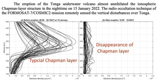
Detection of Vertical Changes in the Ionospheric Electron Density Structures by the Radio Occultation Technique Onboard the FORMOSAT-7/COSMIC2 Mission over the Eruption of the Tonga Underwater Volcano on 15 January 2022

Abstract

A large near-surface perturbation such as the eruption of the Tonga underwater volcano on 15 January 2022 can generate disturbances in the Earth’s atmosphere and ionosphere. It is quite challenging to detect and investigate the disturbances in the vertical direction due to the lack of ground-based instruments, especially in the ocean area. To examine the vertical disturbances due to the Tonga eruption, this study utilizes the radio occultation (RO) technique onboard the satellites of the FORMOSAT-7/COSMIC2 (F7/C2) mission to sound the ionospheric electron density (Ne) profiles in the Central Pacific Ocean area around the eruption. The ionospheric Ne profiles show that the eruption almost annihilated the typical Chapman-layer structure over the eruption in the nighttime on 15 January. The Hilbert–Huang transform was applied to expose the vertical changes in the Ne structures as functions of wavelength and altitude. The analysis shows not only the occurrence of the small-scale disturbances with a wavelength of ~20 km from 100 km to 500 km altitudes, but also the significant attenuation of the structures with a wavelength >50 km, which has never been reported before. The time series of the total electron content from the ground-based Global Navigation Satellite System receiver near the eruption also verifies the significant long-lasting disturbances due to the eruption.

1. Introduction

Large perturbations occurring near the Earth’s surface, such as earthquakes, tsunamis, volcanos, typhoons, and hurricanes, can induce ionospheric disturbances or waves with periods of dozens of minutes that travel away from the origin with a velocity ranging from hundreds to thousands of meters per second [1,2,3,4,5,6,7,8,9,10,11,12]. Most studies utilized the total electron content (TEC) observations from the dense ground-based Global Navigation Satellite System (GNSS) networks to examine the propagation of the disturbances or waves in the horizontal direction. On the other hand, the disturbances or waves propagating upward can penetrate the atmosphere and perturb the ionosphere. Several studies utilized multiple ground-based instruments, such as seismometer, infrasonic system, magnetometer, lidar, high-frequency Doppler sounding system, ground-based GNSS receiver, and ionosonde to detect the vertically propagating disturbances or waves [13,14,15,16,17,18] and reported the significance and complexity of the disturbances originating from the lithosphere.

Investigating the vertical disturbances allows us to understand the wave propagation and dynamic changes in different spheres of the Earth. However, detection and examination of the disturbances in the vertical direction remain challenging because the instruments are rare and installed mainly over the land [19]. The radio occultation (RO) technique onboard the Low-Earth-Orbit (LEO) satellites sounds the ionospheric structure globally, which benefits examining phenomena happening over the ocean, desert, and polar regions, where ground-based instruments are lacking. Several studies utilized the RO technique of the FORMOSAT3/COMSIC (F3/C) mission to examine the vertical disturbances due to large earthquakes and tsunamis [20,21,22,23,24].

The Tonga underwater volcano (20.53°S, 175.38°W) explosively erupted in the middle Pacific Ocean at ~04:15 UT on 15 January 2022 (https://earthquake.usgs.gov/earthquakes/eventpage/pt22015050/executive, accessed on 17 July 2022). The eruption-triggered ionospheric waves and disturbances with a period ranging from dozens of minutes to several hours that propagate in the horizontal direction with a speed of hundreds of meters per second [25,26,27,28,29,30,31]. Such kind of significant perturbations occurring near the Earth’s surface should also disturb the vertical structure of the ionosphere. However, the vertical ionospheric disturbances near the eruption were not reported and addressed yet due to the lack of ground-based instruments over the ocean.

Accordingly, in this study, we analyzed the ionospheric RO electron density (Ne) profiles from the FORMOSAT-7/COSMIC-2 (F7/C2) mission and reported the vertical changes in the ionospheric Ne structure due to the eruption. A minor geomagnetic storm occurred on 14 January (https://wdc.kugi.kyoto-u.ac.jp, accessed on 17 July 2022) that is one day before the eruption. The auroral electrojet (AE) index exceeded 500 nT before 04:00 UT on the eruption day. It was stable (~100 nT) during and several hours after the eruption from ~04:00 UT to ~11:00 UT, which suggests that the possible geomagnetic storm effect on the data is minor. The eruption-induced wind disturbances modulated the E-region current and, in turn, changed the geomagnetic field by ~20 to ~50 nT, mainly over the Pacific. The traveling speed of the wind disturbance was near acoustic (740 m/s) [31]. The tendency of the horizontal component of the geomagnetic field varied gradually from ~04:00 to ~14:00 UT, which suggests that the variation in the background wind field was much weaker than the eruption-induced wind disturbances. This study aims to expose the characteristics of the vertical ionospheric disturbances in various scales over the eruption. The main idea is to apply the RO technique to sense the vertical disturbances remotely over the ocean.

2. Data and Methodology

Six LEO satellites of the F7/C2 mission were launched on 25 June 2019 and were deployed to different orbital planes with a period of ~97 min and an inclination of 24° at 550 km altitude. The Tri-GNSS RO system (TGRS) is the main mission payload of F7/C2, which receives the signals from the GNSS satellites, including GPS, GLONASS, and Galileo systems, and provides more than 4000 ionospheric sounding per day within ±40° latitudes, globally. The TGRS retrieves the Ne structures based on detecting changes in the radio signal transmitted from the GNSS satellites as it passes through the ionosphere. The daily number of the F7/C2 ionospheric RO soundings is near four times more than those of the F3/C mission at low latitudes, which allows scientists to examine the equatorial and low-latitude ionosphere with higher temporal and spatial resolutions [32,33].

Figure 1 shows the distribution of the RO soundings around Tonga on 15 January. The dense RO soundings over the ocean area, where the ground-based multiple instruments are lacking, benefit us in detecting and examining the changes in the vertical ionospheric structures due to the Tonga eruption. On the other hand, for comparing the results from the RO soundings, we also analyzed the total electron content (TEC, 1TEC unit (TECU) = 1 × 10¹⁶ el/m², 0.5 min temporal resolution) from the ground-based GNSS receiver SAMO (13.76°S, 171.74°W) near the eruption. The TEC between the receiver and the geostationary (GEO) satellite operated by the BeiDou Navigation Satellite (BDS) system over the specific location efficiently monitors the perturbations originating from below as a space seismometer [34].

This study utilized the Hilbert–Huang transform (HHT) [35] to analyze the RO profiles and the TEC time series to reveal the changes in the Ne structures in detail. The HHT is a technique that well illustrates the evolution of the TEC waves [36] and capture the vertical disturbances [22,23,37]. The HHT is a data-adaptive time–frequency analysis method without the traditional harmonic assumption that computes the wave amplitude and frequency or wavenumber as functions of time or space [35]. In the time domain, the empirical mode decomposition (EMD) of the HHT decomposes a time series into several components from small to large scales. On the other hand, the Hilbert-spectral analysis can estimate the instantaneous amplitude and phase of each component in the frequency domain. The derivative of the phase function is the instantaneous frequency or wavenumber. In this study, the amplitudes are averaged at each grid of frequency ($f$) and time (t) for constructing the Hilbert spectrum of the TEC time series, $H_{TEC}(f, t)$ [36]. Similarly, the Hilbert spectrum of the vertical RO sounding profiles, $H_{RO}(\lambda , z)$, is the amplitude values being averaged at each altitude (z) and wavelength ($\lambda$) [37]. The marginal spectrum, $n\left(\lambda \right)$, is defined as the summation of the amplitude within a specific altitude interval (z₀ to z₁), $n\left(\lambda \right)={{\displaystyle \int }}_{z0}^{z1}{H}_{RO}(\lambda ,z)dz$ [35].

3. Results

The top three panels in Figure 2 compare the Ne profiles on 15 January around the eruption and those on the two days before. The profiles were collected within an area with a radius of 2000 km centering at 20.54°S, 175.38°W. The profiles illustrate the vertical ionospheric Ne structures, in which the F₂ layer is the primary component, approximating the Chapman-layer structure [38]. It is well known that the lower part of the ionosphere, including the E and F₁ layers (mainly lower than 200 km altitude), is dominated by the photochemical process and vanishes almost in the nighttime due to the high loss rate there. On the other hand, the electron density in the F₂ layer (mainly above 200 km altitude) and above decreases gradually in the nighttime due to the lower loss rate [38]. Therefore, typically, the upper part of the ionosphere attenuates after the sunset, but it is still alive there [39]. The top two panels display the typical diurnal evolution of the ionospheric Ne profile, which is strong in the daytime but weak in the nighttime, on 13 and 14 January. The density profiles are lowest near 16:15 UT, and the Chapman-layer structure becomes pronounced as the dawn comes. It is also typical that the F₂ layer is satiety before the eruption on 15 January (middle panel). However, the F₂ layer seems to be attenuated and the vertical structures are disturbed after the eruption in the afternoon. The typical Chapman-layer structure vanishes almost after 10:00 UT in the nighttime and recovers after ~18:00 UT, that is, near one hour after sunrise.

The bottom two panels of Figure 2 display the Ne profiles in the two nearby areas with a radius of 2000 km centering at 20.54°S, 154.62°E, and at 20.54°S, 145.38°W, respectively, on the western and eastern sides of the volcano on 15 January. The Chapman-layer structure exists in the two areas in both day and night except the hour before sunrise. The ionospheric density is lowest before sunrise typically. The results suggest that the disappearance of the major ionospheric layers for ~8 h over Tonga is a regional phenomenon due to the eruption.

In Figure 3a, the mean Ne profiles in the area centering the eruption show that the ionospheric peak density (N_mF₂) is ~10 × 10⁵ el/cm³, and the peak density height (h_mF₂) is ~330 km during the period between 00:00 UT to 04:15 UT on the three days of 13, 14, and 15 January. The agreement between them suggests that the ionosphere is quite normal before the eruption on 15 January. However, the N_mF₂ deceases significantly, and the Chapman-layer structure is frustrated after the eruption (Figure 3b,c). The N_mF₂ after the eruption from 04:15 UT to 10:00 UT is ~50% lower than that on 13 and 14 January (Figure 3b). Almost the entire ionospheric layers were gone and did not satisfy the typical Chapman layer [38] anymore in the nighttime hours from 10:00 UT to 18:00 UT on 15 January (Figure 3c). Figure 3d shows the recovery of the ionosphere after the sunrise. The h_mF₂ in the daytime on 16 January is slightly higher than that on the other days. Overall, the mean Ne profile is normal one day after the eruption.

To examine the vertical perturbations with shorter wavelengths after the eruption, we collected the Ne profiles during the two periods of 04:15 UT to 10:00 UT (Figure 4) and 10:00 to 16:00 UT (Figure 5), and derived their Hilbert spectra that display the amplitude of the Ne structures as a function of wavelength and altitude. The Hilbert spectrum on 14 January represents the normal condition of the amplitude of the Ne structures in the vertical direction (Figure 4a). The spectrum illustrates that, overall, the amplitude on 15 January (Figure 4b) is weaker than that on 14 January. We subtracted the spectrum on 15 January from that on 14 January (Figure 4c). The difference shows that the structures with a wavelength shorter than ~100 km are enhanced between 150 km to 500 km altitude. However, the structure with a longer wavelength seems weak after the eruption. The bottom two panels of Figure 4 show the marginal spectra on 14 and 15 January. The marginal spectrum is the summation of the amplitude within the altitude interval of z₀ = 150 km to z₁ = 500 km. It can be seen that the amplitude with the shorter/longer wavelength on the eruption day ($n_{eruption}$) is stronger/weaker than that one day before ($n_{normal}$). The relative difference, $(n_{eruption}-n_{normal})/n_{normal}$, shows that the structures with a wavelength shorter than 20 km get stronger by ~50% to ~190% after the eruption. By contrast, the structures with wavelength >100 km decrease by ~40%.

The amplitude during the period between 10:00 UT to 16:00 UT on 14 January (Figure 5a) is also obviously stronger than that in the nighttime on 15 January (Figure 5b). In Figure 5c, the difference between the two spectra also shows that the short-wavelength structures are stronger, but the long-wavelength structures are weaker in the nighttime. In the bottom panels, the marginal spectra display that the amplitude of the structures with wavelength <20 km on 15 January is slightly higher than that on 14 January by ~25%. By contrast, the structure with a wavelength >50 km on 15 January is ~60% weaker than that on 14 January. In short, the short-wavelength structures are stronger but the long-wavelength structures become much weaker after the eruption (Figure 5 and Figure 6), which differs from the characteristics of the vertical ionospheric perturbations triggered by large earthquakes and tsunamis [22,23].

We also analyzed a TEC time series near the eruption to verify the RO results. The TEC of the ground-based receiver SAMO increases significantly after ~04:15 UT, reaches the local maximum at ~04:50, and decreases immediately at ~05:00 UT. Later, the TEC reaches a local minimum at ~05:50 UT, recovers gradually, and reduces further after the sunset at ~07:15 UT (Figure 6a). The comparison of the sudden TEC changes on 15 January and the TEC curvatures on 13 and 12 January (quiet days) shows that the waveform right after the eruption is similar to the typical N-shaped structure in TEC due to the rupture of a large earthquake [21] or a supersonic moon shadow [36]. The period and amplitude of the N-shaped waveform due to the eruption is ~3 h and ~10 TECU, respectively, which are much more significant than the N-shaped structures due to an earthquake or a moon shadow (period of dozens of minutes, amplitude of a few TECU), as reported in the previous studies.

The slope of the TEC between 02:00 UT to 04:00 UT is near −8 TECU/hour in the afternoon before the eruption. However, the TEC changes become much steeper after the eruption. The slope is −39 TECU/hour between 05:00 UT and the minimum at ~05:50 UT. The difference between the TEC value at 04:00 UT and the value near the sunset exceeds −15 TECU at least, which suggests the occurrence of a significant density depression and potentially causes a navigation range error in the order of several meters [40]. The TEC keeps decreasing after the sunset and remains low from ~09:30 until the sunrise. The Hilbert spectrum of the TEC time series, as shown in Figure 6b, illustrates the disturbances with frequencies being higher than 0.02 min⁻¹ (i.e., a period shorter than 50 min) that occurred right after the eruption at 04:15 UT and persisted till ~12:00 UT.

4. Discussion

The Hilbert and marginal spectra of the F7/C2 RO Ne profiles (Figure 4 and Figure 5) illustrate the occurrence of short-wavelength disturbances several hours after the Tonga eruption. Meanwhile, the long-wavelength structures became much weaker. The attenuation of the long-wavelength structures after the eruption (Figure 4 and Figure 5) differs from the vertical disturbances due to large earthquakes and tsunamis [21,22,23]. The Hilbert spectrum of the F3/C RO soundings shows the Ne disturbances induced by the underneath Rayleigh and tsunami waves due to the 31 March 2011 Mw9.0 Tohoku earthquake/tsunami and their post-waves in the entire wavelength band, ranging from several (small scale) to hundreds (large scale) of kilometers in the vertical direction [22]. The spectral analysis of the RO soundings also shows the broadband disturbances that occurred after the Mw8.8 Offshore Maule, Chile, earthquake and tsunami on 27 February 2010 [23]. One F3/C RO sounding profile captured a significant vertical disturbance with a scale of ~150 km in the ionospheric F₂ region due to the Rayleigh wave of the Mw7.8 Nepal earthquake on 25 April 2015 [21]. The RO sounding did not get the chance to detect the small-scale disturbance, because the Nepal earthquake occurred near the end of the operational period of the F3/C mission when the number of the daily profiles was small. Anyway, the previous events show the ionosphere being perturbed in both small and large scales. However, after the Tonga eruption, the small-scale disturbances were significant, but the large-scale structures became weaker (Figure 4 and Figure 5). The example of the time series of the ground-based GNSS TEC near Tonga and its spectrum (Figure 6) verify the small-scale structures being significant several hours after the eruption. The persistent small-scale disturbances with the vertical wavelength ranging from several to tens of kilometers (Figure 4 and Figure 5) and the period ranging from several to ~dozens of minutes (Figure 6) can be attributed to the long-lasting tail or atmospheric resonance [8]. Note that the RO data are sparsely distributed and record snapshots of the vertical disturbance [21]. The RO technique can detect the intensity and scales of disturbances, but it remains challenging to trace the vertical propagation of a transient disturbance.

The attenuation of the long-wavelength structures (Figure 4 and Figure 5) relates to the disappearance of the major ionospheric layers after the eruption. It seems almost the entire ionospheric layers being blown away, and the typical Chapman-layer structure no longer exists over the volcano (Figure 2 and Figure 3). The disappearance is a depression in the ionospheric electron density with a duration of ~8 h (~10:00 to ~18:00 UT) and a horizontal scale of ~4000 km. The TEC time series decreased significantly after the eruption and also remained low in the whole night (Figure 6) verifying the depression. Typically, the F₂ layer can become weaker after sunset, but it still alive in the nighttime because the transport process dominates the F₂ layer and the loss rate of plasma is low [38]. However, the disappearance of the Chapman-layer structure over the eruption in the nighttime (Figure 2 and Figure 3) is unexpected.

A large ionospheric hole occurred over the tsunami source area of the Tohoku earthquake [41,42]. The hole is a sudden decrease in TEC (decrease by >5 TECU) on the hundred-kilometer scale in the horizontal direction after the rupture and lasts near one hour. The meter-scale sea surface perturbation due to the giant tsunami punched the atmosphere and induced the ionospheric hole. In the vertical direction, the F3/C RO soundings recorded that the vertical Ne structures fluctuated largely, and the Chapman-layer structure still existed after the rupture of the Tohoku earthquake [22]. The extreme explosive eruption blew the molecular particles from lower altitudes to the upper atmosphere, which changed the thermospheric composition, reduced the ratio of the atomic and molecular densities (e.g., [O]/[N2]), and further increased the loss rate of plasma in the ionosphere. That is the main reason for the disappearance of the typical Chapman-layer structures for several hours after the eruption. The disappearance of the major layers causes the Ne depression due to the explosive eruption of the Tonga volcano, which is much more significant than the effect of the M9.0 Tohoku earthquake and tsunami on the upper atmosphere.

The rapid increase and decrease in the TEC time series (Figure 6a), i.e., the large N-shape waveform, suggests the occurrence of a blast wave [43] due to the explosive eruption. The local maximum at ~04:50 UT and minimum at ~05:50 UT of the TEC time series indicate the positive and negative phases of the pressure profile of a blast wave near the eruption. The significant positive change is the over-pressurization impulse of the blast. The negative phase represents the low density, which is one of the reasons for the depression in the ionospheric Ne density after the eruption. On the other hand, the positive phase is the near-instantaneous air compression that causes the high plasma-neutral collision frequency and increases the loss rate of plasma [38], which can also contribute to the depression as the wavefront is passing through.

Note that the upward-propagating disturbances such as acoustic and internal gravity waves are formed not only during volcanic eruptions, earthquakes, and tsunamis, but also during meteorological storms, solar eclipses, and the passage of the solar terminator [17,44,45]. The vertical disturbances due to the astronomical phenomena can be also further examined.

5. Conclusions

The radio occultation (RO) technique onboard the Low-Earth-Orbit (LEO) satellites of the FORMOSAT-7/COSMIC2 (F7/C2) mission detected the vertical disturbances in the ionospheric electron density (Ne) due to the explosive eruption of the Tonga underwater volcano on 15 January 2022. The spectral analysis of the dense RO Ne sounding profiles reveals that the disturbances with the vertical wavelength less than ~25 km are significant over the volcano within ~12 h after the eruption. By contrast, the Ne structures with longer wavelengths were attenuated significantly, which can be attributed to the disappearance of the typical Chapman-layer structure of the ionosphere after the eruption in the nighttime.

The disappearance of the major ionosphere layers detected by the RO technique after the eruption reveals the occurrence of depression in the ionosphere electron density over Tonga. The depression occurred in an area with a diameter of ~4000 km during the whole night of 15–16 January. The sharp decrease (−39 TECU/hour) in the TEC after the eruption verifies the depression around the eruption. The evidence from the F7/C2 RO soundings for the first time reveals that a large near-surface perturbance can almost annihilate the major ionospheric layers, which was never found in previous large earthquake or tsunami events. The primary injuries of ionosphere caused by the blast due to the explosive eruption is the disappearance of the Chapman layer and large disturbances. The impact of such large-scale changes on the dynamics of the ionosphere and thermosphere can be further examined.

References

1. Liu, J.Y.; Tsai, Y.B.; Chen, S.W.; Lee, C.P.; Chen, Y.C.; Yen, H.Y.; Chang, W.Y.; Liu, C. Giant ionospheric disturbances excited by the M9.3 Sumatra earthquake of 26 December 2004. Geophys. Res. Lett. 2006, 33, L02103. [Google Scholar] [CrossRef]
2. Liu, J.-Y.; Chen, C.-H.; Lin, C.-H.; Tsai, H.-F.; Chen, C.-H.; Kamogawa, M. Ionospheric disturbances triggered by the 11 March 2011 M9.0 Tohoku earthquake. J. Geophys. Res. Earth Surf. 2011, 116, A06319. [Google Scholar] [CrossRef]
3. Otsuka, Y.; Kotake, N.; Tsugawa, T.; Shiokawa, K.; Ogawa, T.; Effendy; Saito, S.; Kawamura, M.; Maruyama, T.; Hemmakorn, N.; et al. GPS detection of total electron content variations over Indonesia and Thailand following the 26 December 2004 earthquake. Earth Planets Space 2006, 58, 159–165. [Google Scholar] [CrossRef]
4. Tsugawa, T.; Saito, A.; Otsuka, Y.; Nishioka, M.; Maruyama, T.; Kato, H.; Nagatsuma, T.; Murata, K.T. Ionospheric disturbances detected by GPS total electron content observation after the 2011 off the Pacific coast of Tohoku Earthquake. Earth Planets Space 2011, 63, 875–879. [Google Scholar] [CrossRef]
5. Chen, C.H.; Saito, A.; Lin, C.C.H.; Liu, J.Y.; Tsai, H.F.; Tsugawa, T.; Otsuka, Y.; Nishioka, M.; Matsumura, M. Long-distance propagation of ionospheric disturbance generated by the 2011 off the Pacific coast of Tohoku earthquake. Earth Planets Space 2011, 63, 881–884. [Google Scholar] [CrossRef]
6. Nishioka, M.; Tsugawa, T.; Kubota, M.; Ishii, M. Concentric waves and short-period oscillations observed in the ionosphere after the 2013 Moore EF5 tornado. Geophys. Res. Lett. 2013, 40, 5581–5586. [Google Scholar] [CrossRef]
7. Chou, M.Y.; Lin, C.C.H.; Yue, J.; Tsai, H.F.; Sun, Y.Y.; Liu, J.Y.; Chen, C.H. Concentric traveling ionosphere disturbances triggered by Super Typhoon Meranti (2016). Geophys. Res. Lett. 2017, 44, 1219–1226. [Google Scholar] [CrossRef]
8. Chou, M.-Y.; Cherniak, I.; Lin, C.C.; Pedatella, N. The Persistent Ionospheric Responses Over Japan After the Impact of the 2011 Tohoku Earthquake. Space Weather 2020, 18, e2019SW002302. [Google Scholar] [CrossRef]
9. Heki, K. Explosion energy of the 2004 eruption of the Asama Volcano, central Japan, inferred from ionospheric disturbances. Geophys. Res. Lett. 2006, 33, L14303. [Google Scholar] [CrossRef]
10. Dautermann, T.; Calais, E.; Mattioli, G. Global Positioning System detection and energy estimation of the ionospheric wave caused by the 13 July 2003 explosion of the Soufrière Hills Volcano, Montserrat. J. Geophys. Res. Earth Surf. 2009, 114, B02202. [Google Scholar] [CrossRef]
11. Shults, K.; Astafyeva, E.; Adourian, S. Ionospheric detection and localization of volcano eruptions on the example of the April 2015 Calbuco events. J. Geophys. Res. Space Phys. 2016, 121, 10303–10315. [Google Scholar] [CrossRef]
12. Astafyeva, E. Ionospheric detection of natural hazards. Rev. Geophys. 2019, 57, 1265–1288. [Google Scholar] [CrossRef]
13. Liu, J.-Y.; Sun, Y.-Y. Seismo-traveling ionospheric disturbances of ionograms observed during the 11 March 2011 M9.0 Tohoku earthquake. Earth Planets Space 2011, 63, 897–902. [Google Scholar] [CrossRef]
14. Liu, J.Y.; Chen, C.H.; Sun, Y.Y.; Tsai, H.F.; Yen, H.Y.; Chum, J.; Lastovicka, J.; Yang, Q.S.; Chen, W.S.; Wen, S. The vertical propagation of disturbances triggered by seismic waves of the 11 March 2011 M9.0 Tohoku earthquake over Taiwan. Geophys. Res. Lett. 2016, 43, 1759–1765. [Google Scholar] [CrossRef]
15. Maruyama, T.; Tsugawa, T.; Kato, H.; Saito, A.; Otsuka, Y.; Nishioka, M. Ionospheric multiple stratifications and irregularities induced by the 2011 off the Pacific coast of Tohoku Earthquake. Earth Planets Space 2011, 63, 869–873. [Google Scholar] [CrossRef]
16. Maruyama, T.; Yusupov, K.; Akchurin, A. Ionosonde tracking of infrasound wavefronts in the thermosphere launched by seismic waves after the 2010 M8.8 Chile earthquake. J. Geophys. Res. Space Phys. 2016, 121, 2683–2692. [Google Scholar] [CrossRef]
17. Wang, J.; Zuo, X.; Sun, Y.-Y.; Yu, T.; Wang, Y.; Qiu, L.; Mao, T.; Yan, X.; Yang, N.; Qi, Y.; et al. Multilayered sporadic-E response to the annular solar eclipse on June 21, 2020. Space Weather 2021, 19, e2020SW002643. [Google Scholar] [CrossRef]
18. Borchevkina, O.P.; Kurdyaeva, Y.A.; Dyakov, Y.A.; Karpov, I.V.; Golubkov, G.V.; Wang, P.K.; Golubkov, M.G. Disturbances of the Thermosphere and the Ionosphere during a Meteorological Storm. Atmosphere 2021, 12, 1384. [Google Scholar] [CrossRef]
19. Chen, C.-H.; Sun, Y.-Y.; Lin, K.; Zhou, C.; Xu, R.; Qing, H.; Gao, Y.; Chen, T.; Wang, F.; Yu, H.; et al. A new instrumental array in Sichuan, China, to monitor vibrations and perturbations of the lithosphere, atmosphere and ionosphere. Surv. Geophys. 2021, 42, 1425–1442. [Google Scholar] [CrossRef]
20. Coïsson, P.; Lognonné, P.; Walwer, D.; Rolland, L.M. First tsunami gravity wave detection in ionospheric radio occultation data. Earth Space Sci. 2015, 2, 125–133. [Google Scholar] [CrossRef]
21. Sun, Y.-Y.; Liu, J.-Y.; Lin, C.-Y.; Tsai, H.-F.; Chang, L.C.; Chen, C.-Y.; Chen, C.-H. Ionospheric F2 region perturbed by the 25 April 2015 Nepal earthquake. J. Geophys. Res. Space Phys. 2016, 121, 5778–5784. [Google Scholar] [CrossRef]
22. Liu, J.-Y.; Chen, C.-Y.; Sun, Y.-Y.; Lee, I.-T.; Chum, J. Fluctuations on vertical profiles of the ionospheric electron density perturbed by the 11 March, 2011 M9.0 Tohoku earthquake and tsunami. GPS Solut. 2019, 23, 76. [Google Scholar] [CrossRef]
23. Sun, Y.-Y. GNSS brings us back on the ground from ionosphere. Geosci. Lett. 2019, 6, 14. [Google Scholar] [CrossRef]
24. Yan, X.; Sun, Y.-Y.; Yu, T.; Liu, J.-Y.; Qi, Y.; Xia, C.; Zuo, X.; Yang, N. Stratosphere perturbed by the 2011 Mw9.0 Tohoku earthquake. Geophys. Res. Lett. 2018, 45, 10050–10056. [Google Scholar] [CrossRef]
25. Themens, D.R.; Watson, C.; Žagar, N.; Vasylkevych, S.; Elvidge, S.; McCaffrey, A.; Prikryl, P.; Reid, B.; Wood, A.; Jayachandran, P.T. Global Propagation of Ionospheric Disturbances Associated With the 2022 Tonga Volcanic Eruption. Geophys. Res. Lett. 2022, 49, e2022GL098158. [Google Scholar] [CrossRef]
26. Lin, J.; Rajesh, P.K.; Lin, C.C.H.; Chou, M.; Liu, J.; Yue, J.; Hsiao, T.; Tsai, H.; Chao, H.; Kung, M. Rapid Conjugate Appearance of the Giant Ionospheric Lamb Wave Signatures in the Northern Hemisphere After Hunga-Tonga Volcano Eruptions. Geophys. Res. Lett. 2022, 49, e2022GL098222. [Google Scholar] [CrossRef]
27. Astafyeva, E.; Maletckii, B.; Mikesell, T.D.; Munaibari, E.; Ravanelli, M.; Coisson, P.; Manta, F.; Rolland, L. The 15 January 2022 Hunga Tonga Eruption History as Inferred From Ionospheric Observations. Geophys. Res. Lett. 2022, 49, e2022GL098827. [Google Scholar] [CrossRef]
28. Chen, C.-H.; Zhang, X.; Sun, Y.-Y.; Wang, F.; Liu, T.-C.; Lin, C.-Y.; Gao, Y.; Lyu, J.; Jin, X.; Zhao, X.; et al. Individual Wave Propagations in Ionosphere and Troposphere Triggered by the Hunga Tonga-Hunga Ha’apai Underwater Volcano Eruption on 15 January 2022. Remote Sens. 2022, 14, 2179. [Google Scholar] [CrossRef]
29. Zhang, S.-R.; Vierinen, J.; Aa, E.; Goncharenko, L.P.; Erickson, P.J.; Rideout, W.; Coster, A.J.; Spicher, A. 2022 Tonga volcanic eruption induced global propagation of ionospheric disturbances via Lamb waves. Front. Astron. Space Sci. 2022, 9, 871275. [Google Scholar] [CrossRef]
30. Saito, S. Ionospheric disturbances observed over Japan following the eruption of Hunga Tonga-Hunga Ha’apai on 15 January 2022. Earth Planets Space 2022, 74, 57. [Google Scholar] [CrossRef]
31. Sun, Y.-Y.; Chen, C.-H.; Zhang, P.-Y.; Li, S.; Xu, H.-R.; Yu, T.; Lin, K.; Mao, Z.; Zhang, D.; Lin, C.-Y.; et al. Explosive eruption of the Tonga underwater volcano modulates the ionospheric E-region current on 15 January 2022. Geophys. Res. Lett. 2022, 49, e2022GL099621. [Google Scholar] [CrossRef]
32. Lin, C.-Y.; Lin, C.C.-H.; Liu, J.-Y.; Rajesh, P.K.; Matsuo, T.; Chou, M.-Y.; Tsai, H.-F.; Yeh, W.-H. The early results and validation of FORMOSAT-7/COSMIC-2 space weather products: Global ionospheric specification and Ne-aided Abel electron density profile. J. Geophys. Res. Space Phys. 2020, 125, e2020JA028028. [Google Scholar] [CrossRef]
33. Liu, T.J.-Y.; Lin, C.C.; Lin, C.-Y.; Lee, I.-T.; Sun, Y.-Y.; Chen, S.-P.; Chang, F.-Y.; Rajesh, P.K.; Hsu, C.-T.; Matsuo, T.; et al. Retrospect and prospect of ionospheric weather observed by FORMOSAT-3/COSMIC and FORMOSAT-7/COSMIC-2. Terr. Atmos. Ocean. Sci. 2022, 33, 20. [Google Scholar] [CrossRef]
34. Chen, C.-H.; Sun, Y.-Y.; Xu, R.; Lin, K.; Wang, F.; Zhang, D.; Zhou, Y.; Gao, Y.; Zhang, X.; Yu, H.; et al. Resident waves in the ionosphere before the M6.1 Dali and M7.3 Qinghai earthquakes of 21–22 May 2021. Earth Space Sci. 2022, 9, e2021EA002159. [Google Scholar] [CrossRef]
35. Huang, N.E.; Shen, Z.; Long, S.R.; Wu, M.C.; Shih, H.H.; Zheng, Q.; Yen, N.-C.; Tung, C.C.; Liu, H.H. The empirical mode decomposition and the Hilbert spectrum for nonlinear and non-stationary time series analysis. Proc. R. Soc. Lond. Ser. A-Math. Phys. Eng. Sci. 1998, 454, 903–995. [Google Scholar] [CrossRef]
36. Sun, Y.-Y.; Shen, M.M.; Tsai, Y.-L.; Lin, C.-Y.; Chou, M.-Y.; Yu, T.; Lin, K.; Huang, Q.; Wang, J.; Qiu, L.; et al. Wave steepening in ionospheric total electron density due to the 21 August 2017 total solar eclipse. J. Geophys. Res. Space Phys. 2021, 126, e2020JA028931. [Google Scholar] [CrossRef]
37. Sun, Y.-Y.; Oyama, K.-I.; Liu, J.-Y.; Jhuang, H.-K.; Cheng, C.-Z. The neutral temperature in the ionospheric dynamo region and the ionospheric F region density during Wenchuan and Pingtung Doublet earthquakes. Nat. Hazards Earth Syst. Sci. 2011, 11, 1759–1768. [Google Scholar] [CrossRef]
38. Davies, K. Ionospheric Radio; Peregrinus: London, UK, 1990. [Google Scholar]
39. Wang, J.; Sun, Y.-Y.; Yu, T.; Wang, Y.; Mao, T.; Yang, H.; Xia, C.; Yan, X.; Yang, N.; Huang, G.; et al. Convergence effects on the ionosphere during and after the annular solar eclipse on 21 June 2020. J. Geophys. Res.-Space Phys. 2022, 127, e2022JA030471. [Google Scholar] [CrossRef]
40. Chou, M.-Y.; Shen, M.-H.; Lin, C.C.H.; Yue, J.; Chen, C.-H.; Liu, J.-Y.; Lin, J.-T. Gigantic circular shock acoustic waves in the ionosphere triggered by the launch of FORMOSAT-5 satellite. Space Weather 2018, 16, 172–184. [Google Scholar] [CrossRef]
41. Kakinami, Y.; Kamogawa, M.; Tanioka, Y.; Watanabe, S.; Gusman, A.R.; Liu, J.-Y.; Watanabe, Y.; Mogi, T. Tsunamigenic ionospheric hole. Geophys. Res. Lett. 2012, 39, L00G27. [Google Scholar] [CrossRef]
42. Kamogawa, M.; Orihara, Y.; Tsurudome, C.; Tomida, Y.; Kanaya, T.; Ikeda, D.; Gusman, A.R.; Kakinami, Y.; Liu, J.-Y.; Toyoda, A. A possible space-based tsunami early warning system using observations of the tsunami ionospheric hole. Sci. Rep. 2016, 6, 37989. [Google Scholar] [CrossRef] [PubMed]
43. Shirbhate, P.A.; Goel, M.D. A Critical Review of Blast Wave Parameters and Approaches for Blast Load Mitigation. Arch. Comput. Methods Eng. 2020, 28, 1713–1730. [Google Scholar] [CrossRef]
44. Borchevkina, O.P.; Adamson, S.O.; Dyakov, Y.A.; Karpov, I.V.; Golubkov, G.V.; Wang, P.-K.; Golubkov, M.G. The Influence of Tropospheric Processes on Disturbances in the D and E Ionospheric Layers. Atmosphere 2021, 12, 1116. [Google Scholar] [CrossRef]
45. Song, Q.; Ding, F.; Wan, W.; Ning, B.; Liu, L.; Zhao, B.; Li, Q.; Zhang, R. Statistical study of large-scale traveling ionospheric disturbances generated by the solar terminator over China. J. Geophys. Res. Space Phys. 2013, 118, 4583–4593. [Google Scholar] [CrossRef]
Figure 1. Location of the ionospheric radio occultation (RO) electron density (Ne) soundings (blue dots) within 2000 km away from the Tonga eruptions (red pentagram). Each dot indicates the averaged longitude and latitude of the tangent points of each RO sounding. The triangle is the groundbased GNSS receiver SAMO (13.76°S, 171.74°W). The red dot indicates the location of the ionosphere pierce point (at 350 km altitude) of the total electron content (TEC) between the receiver and the BeiDou Navigation Satellite System geostationary satellite C01.
Remotesensing 14 04266 g001
Figure 2. Top three panels: the ionospheric RO Ne profiles within the radius of 2000 km centering at 20.54°S, 175.38°W (over the eruption) on 13, 14, and 15 January. The Ne value of each profile at 100 km altitude corresponds to its universal time. The vertical red line indicates the eruption on 15 January. The vertical blue lines indicate the sunset and sunrise at ~19:30 LT and ~05:00 LT, respectively (https://www.timeanddate.com/sun/tonga/nukualofa, accessed on 17 July 2022). The red rectangle denotes the Ne profiles without the typical Chapman-layer structure mainly during the period between 10:00–18:00 UT on 15 January. Bottom two panels: the Ne profiles within the radius of 2000 km centering at 20.54°S, 154.62°E (western side of the eruption) and 20.54°S, 145.38°W (eastern side of the eruption) on 15 January.
Remotesensing 14 04266 g002
Figure 3. Comparison of the mean Ne profiles (a) before and (bd) after the eruption on 15 January and those on the two days before (13 and 14 January) and the one day after (16 January). The error bar is the standard deviation of the Ne values at each altitude. The F2 layer vanished almost during the period between 10:00–18:00 UT.
Remotesensing 14 04266 g003
Figure 4. Hilbert spectra of Ne profiles from 04:15 UT to 10:00 UT on (a) 14 and (b) 15 January (eruption day). (c) Difference between the spectra on the eruption day and one day before. The contour line sketched the value of 0 el/cm3. (d) The black and red curves are the marginal spectra on 14 ( n n o r m a l ) and 15 January ( n e r u p t i o n ), respectively. (e) Relative difference between the marginal spectra that is defined as ( n e r u p t i o n n n o r m a l ) / n n o r m a l .
Remotesensing 14 04266 g004
Figure 5. Hilbert spectra of Ne profiles from 10:00 UT to 16:00 UT on (a) 14 and (b) 15 January (eruption day). (c) Difference between the spectra on the eruption day and one day before. The contour line sketched the value of 0 el/cm3. (d) The black and red curves are the marginal spectra on 14 ( n n o r m a l ) and 15 January ( n e r u p t i o n ), respectively. (e) Relative difference between the marginal spectra that is defined as ( n e r u p t i o n n n o r m a l ) / n n o r m a l .
Remotesensing 14 04266 g005
Figure 6. (a) The time series of TEC between the receiver SAMO and the BDS C01 on 15 January (black solid line) and the two qiuet days of 13 (gray solid line) and 12 January (gray dash line). The data are unavailable on 14 January. The vertical red line indicates the eruption. The two dash blue lines indicate the sunset and sunrise. (b) The corresponding Hilbert spectrum of the TEC time series on 15 January.
Remotesensing 14 04266 g006
Publisher’s Note: MDPI stays neutral with regard to jurisdictional claims in published maps and institutional affiliations.