MID: A Novel Mountainous Remote Sensing Imagery Registration Dataset Assessed by a Coarse-to-Fine Unsupervised Cascading Network

Abstract

The geometric registration of mountainous remote sensing images is always a challenging project, as terrain fluctuations increase the complexity. Deep learning, with its superior computing power and data-driven nature, promises to solve this problem. However, the lack of an appropriate dataset limits the development of deep learning technology for mountainous remote sensing image registration, which it still an unsolved problem in photogrammetry and remote sensing. To remedy this problem, this paper presents a manually constructed imagery dataset of mountainous regions, called the MID (mountainous imagery dataset). To create the MID, we use 38 images from the Gaofen-2 satellite developed by China and generated 4093 pairs of reference and sensed image patches, making this the first real mountainous dataset to our knowledge. Simultaneously, we propose a fully unsupervised, convolutional-network-based iterative registration scheme for the MID. First, the large and global deformation of the reference and sensed images is reduced using an affine registration module, generating the coarse alignment. Then, the local and varied distortions are learned and eliminated progressively using a hybrid dilated convolution (HDC)-based encoder–decoder module with multistep iterations, achieving fine registration results. The HDC aims to increase the receptive field without blocking the artifacts, allowing for the continuous characteristics of the mountainous images of a local region to be represented. We provide a performance analysis of some typical registration algorithms and the developed approach for the MID. The proposed scheme gives the highest registration precision, achieving the subpixel alignment of mountainous remote sensing images. Additionally, the experimental results demonstrate the usability of the MID, which can lay a foundation for the development of deep learning technology in large mountainous remote sensing image registration tasks.

1. Introduction

More often than not, the application of remote sensing data, such as image fusion, change detection, and image mosaic data, requires the employed images to be in the same coordinate system, i.e., the same surface features in the same position [1]. However, such a condition is sometimes quite challenging to be accomplished for raw satellite image pairs, as the available remote sensing images may be collected from different satellite sensors, may be multitemporal, or may have inconsistent acquisition angles [2,3], making the geometric registration an indispensable preprocessing step [4].

Over the past decades, quite a few technologies have been developed for remote sensing image registration, which are routinely classified into intensity-based (area-based), feature-based, and hybrid methods [4,5]. The conventional intensity-based approaches directly employ the intensity to iteratively search for the optimal parameters of the specified transformation model [6]. The similarity measure is the key component, such as normalized cross-correlation (NCC) [6], mutual information (MI) [7], and phase congruency (PC) approaches [8]. The intensity-based algorithms with high-precision alignment as the original image information can be adopted without any error accumulation. However, most of them are sensitive to large rotations and scale differences and are quite time-consuming [3]. Compared with the traditional ones, the optical flow estimation approach applied to remote sensing image registration is relatively novel [9,10], of which the product is a per-pixel displacement field. The very local and variable deformations due to terrain elevation can be eliminated in mountainous regions because of the advantages of per-pixel computation [11,12]. However, occlusion is always troublesome when aiming for accurate calculations, as it refers to land-use or land-cover (LULC) changes in remote sensing images [10,13]. Additionally, it exhibits the limitation of containing large deformations.

Unlike the intensity-based method, another method adopts some remarkable and invariant geometric features (e.g., feature points, polylines, and polygons) for alignment instead of the original image, which is the feature-based approach [14]. It is widely applied for heterogeneous image alignment, such as for optical and synthetic aperture radar (SAR) image registration [15], optical and infrared images alignment [16], and optical and LiDAR image registration [17]. It generally demonstrates higher efficiency than the intensity-based approach; meanwhile, the algorithm sometimes provides poor registration for errors in the process of extracting or matching features, even regarding the position of the matched features [4]. For the hybrid algorithm, it generally points to the combination of two or more different alignment commands, most of which are solved in a serial computation [18,19]. Aiming at eliminating the large deformation between the reference and sensed images, feature-based technologies are commonly used [20], such as the scale-invariant feature transform (SIFT) [21], sped-up robust features (SURF) [22], and oriented fast and rotated brief (ORB) methods [23]. The intensity-based algorithm is assigned to improve the accuracy via the CC (cross-correlation) [24], MI, and phase-based correlation approaches, among others. These combinations usually result in high-precision geometric registration as a successive improvement from coarse-to-fine resolutions [7,25,26]. However, the combinations are more time-consuming than the intensity-based or feature-based algorithm. From the above discussion, based on the traditional algorithms, the high-precision alignment of mountainous remote sensing images is difficult to achieve, as the positional relationship is complicated.

Recently, with the transition of deep learning technology from computer vision to the remote sensing field [2,27], some innovations have been introduced to the conventional algorithms [28,29,30], again allowing remote sensing image registration. The deep-learning-based algorithm can automatically learn high-level features, supplementing the conventional geometric features [31,32,33,34]. Moreover, its particular feedback scheme is beneficial for feature extraction, guided by the result of the feature matching [14]. Therefore, deep learning technology, as represented by a convolutional network, can achieve more features with high position accuracy and give a better matching performance than traditional techniques [35,36,37]. Additionally, some algorithms take advantage of the powerful deep learning computation potential, directly learning the mapping function for the spatial alignment of two scenes covering the same region [38,39]. This approach could be concretely comprehended using supervised and unsupervised learning [40,41]. The key point of supervised registration is the ground truth information, such as for the manual matching labels [38], real deformation field [42], and geometric transform matrix [39]. Additionally, guided by its supervised manner, the transformation matrix is creatively transformed into a regression problem [39,43]. For example, a dual DenseNet [44] (D-DenseNet) model was proposed in [39] to regress the corner displacement by subsequently calculating the projection transformation matrix of the corresponding coordinates. From our perspective, obtaining the ground truth alignment information is challenging unless performing the simulation experiment, which cannot present the real spatial relationship of the satellite images. As for unsupervised deep learning, real reference information is not necessary. When applied for image registration, it employs a spatial transformation network to warp the sensed image to the coordinate system of the reference image without any human annotations [40,45,46]. In [47], the end-to-end training of a deep learning model was employed to couple the linear and deformable registration problems. Vakalopoulou et al. constructed a similar convolutional neural network (CNN) architecture for remote sensing imagery alignment, which is completely unsupervised [48]. In [45], a multistep unsupervised deformable image registration approach was proposed with a specified maximum displacement in advance, aligning the given image pairs through an iterative process. This registration strategy is popular in medical image registration, although it requires more process steps to achieve fine results [49,50]. Thus, the unsupervised algorithms always take the flat regions in remote sensing field, including urban and suburban scenes, as the main experimental data, while the deformation is more complicated in mountainous images as they require significant nonlinear spatial mapping.

Inspired by the above observation and conclusion, the unsupervised learning-based pixel-by-pixel registration method promises to solve the mountainous remote sensing image alignment problem. Thus, with a newly constructed imagery dataset, we propose to advance the mountainous remote sensing image registration process based on an unsupervised deep learning framework, taking advantage of the coarse-to-fine resolution strategy and multistep iterations. The contributions of this work are summarized as follows:

(1)

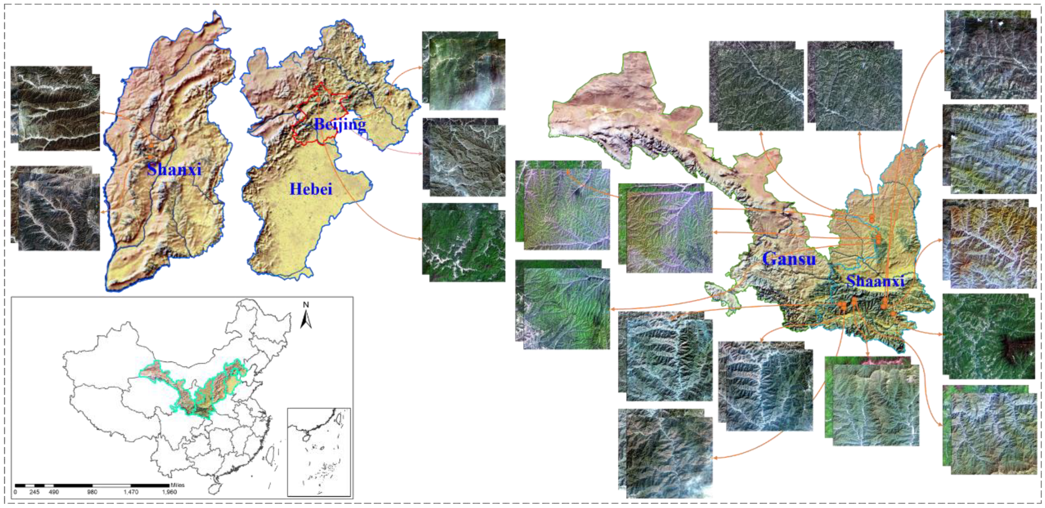
First, for the first time, a mountainous remote sensing imagery dataset (MID) for geometric registration is constructed. The dataset consists of 4093 pairs of image patches located in some specified mountains in China;

(2)

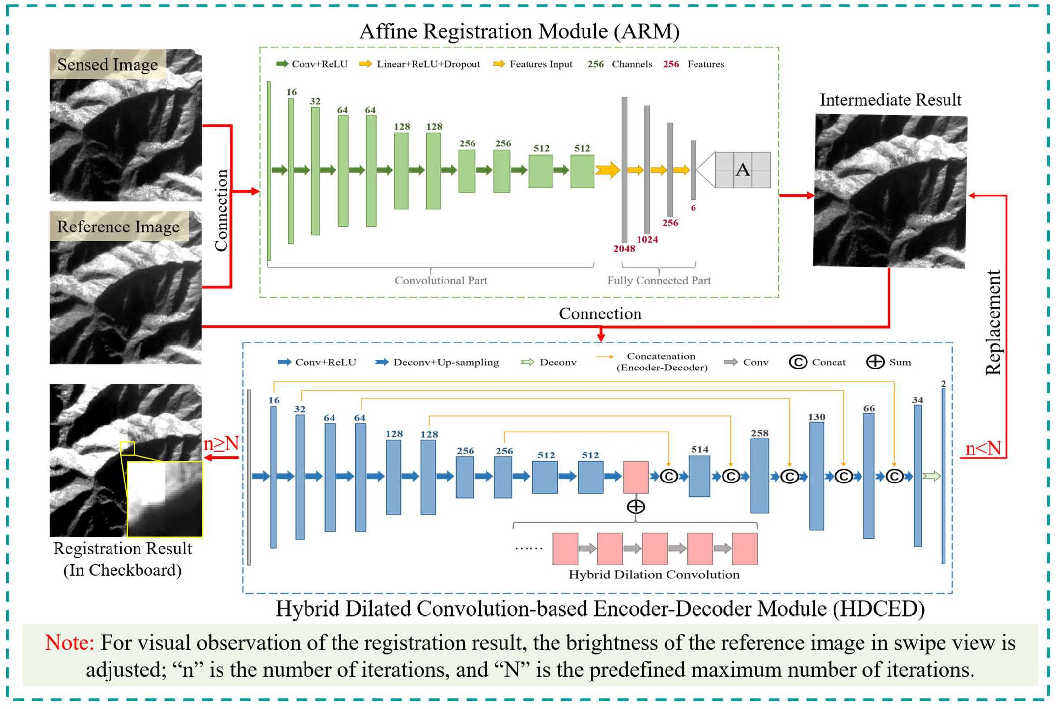
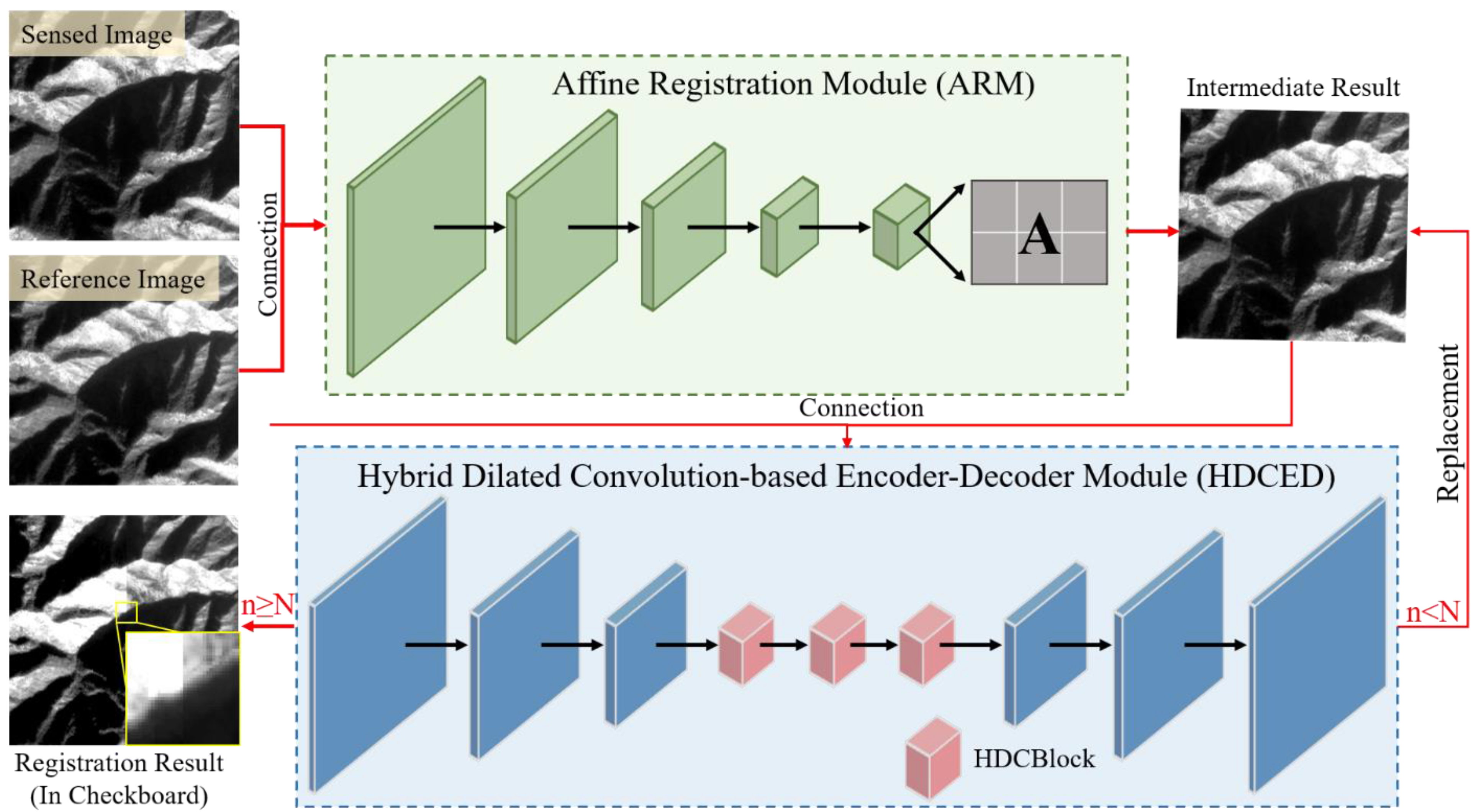
Then, a coarse-to-fine unsupervised cascading convolutional network is developed, consisting of an affine registration module (ARM) and an iterative hybrid dilation convolution-based encoder–decoder (HDCED) module. The entire network is trained in an end-to-end manner, and the previous result is always connected to the reference image as the input of the subsequent process.

The remainder of the paper is organized as follows. The MID dataset is introduced in Section 2. Section 3 presents in detail the proposed method for mountainous remote sensing image registration. To demonstrate the performance of the proposed algorithm as well as some of the typical approaches for the MID, an experimental analysis is given in Section 4. Section 5 discusses the parameter settings and limitations of the proposed algorithm based on the MID dataset. Finally, we conclude the paper and the prospects are summarized in Section 6.

2. The Mountainous Remote Sensing Imagery Dataset (MID)

It is worth noting that there is not a public and sufficient dataset consisting of real remote sensing images for geometric registration yet, especially covering mountainous regions. This is the biggest obstacle to the development of deep learning in this field [27]. Moreover, the public and unified dataset performs well in the fair evaluation of different alignment schemes. Under these circumstances, we established a real MID. It will be publicly available online and could be utilized freely for remote sensing image registration and comparisons of different alignment algorithms.

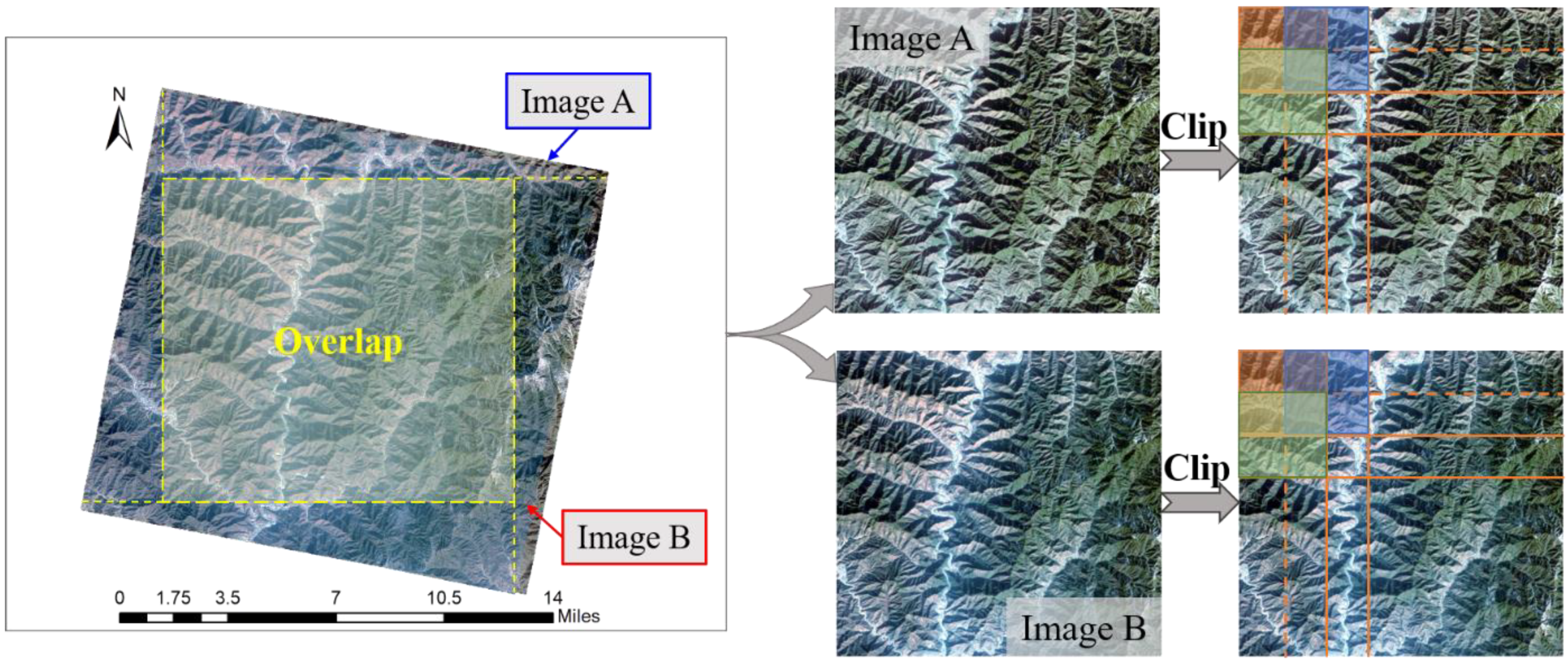
2.1. Construction of the MID

There are some existing public remote sensing imagery datasets with different spatial resolutions and abundant surface features. One dataset (https://github.com/MountainAndGhost/remote-sensing-images-registration-dataset, accessed on 27 September 2020) consists of three subdatasets, including 396 pairs of images with a spatial resolution of 0.23 m, 420 pairs of images mainly covering farmland regions with a 3.75 m spatial resolution, and the last one with a 30 m resolution containing 165 pairs of images. All images to be registered are simulated; that is to say, the sensed image is produced by transforming the reference image with a specified matrix. It cannot accurately represent the real deformation of two raw satellite imageries. The ISPRS IKONOS dataset (https://www.isprs.org/data/ikonos/default.aspx, accessed on 29 March 2021) provides one bitemporal pair of high-resolution ($1 \mathrm{m}\times 1 \mathrm{m}$) images, only covering the urban region with dense high-rise buildings. Differing from them, the real remote sensing images covering mountainous regions have more complex and varied deformations, which cannot be described using these existed datasets. Thus, we construct a real mountainous remote sensing imagery dataset with dozens of multitemporal Gaofen-2 satellite image pairs.

As one of the optical satellites independently developed in China, the Gaofen-2 satellite produces multispectral and panchromatic images with respective ground sampling distances (GSDs) of 4 m and 1 m [51]. We used 38 scenes covering mountains mainly in Beijing, Shanxi, and Shaanxi provinces, China (Figure 1). Most of the selected images are located in the south of Shaanxi province, where Qinling is found. The selection principle is that the images should be as cloud-free as possible, and the imaging time for two images in a pair should be relatively close (shown in

Table 1. The imaging time of two images in each pair for MID construction.

1	2	3	4	5	6	7	8	9	10
11-11-2021	28-05-2020	09-06-2017	22-11-2021	13-01-2017	25-04-2020	19-10-2020	02-04-2016	29-09-2021	29-09-2021
27-10-2021	08-05-2021	01-07-2021	13-01-2017	22-11-2021	25-04-2020	02-04-2016	19-10-2020	09-05-2021	09-05-2021
11	12	13	14	15	16	17	18	19
29-09-2021	29-09-2021	29-09-2021	09-05-2021	29-09-2021	26-01-2021	11-01-2021	04-12-2019	05-12-2016
09-05-2021	09-05-2021	09-05-2021	29-09-2021	09-05-2021	11-01-2021	26-01-2021	16-02-2020	26-10-2018

) or the vegetation in the image should have a similar growth state (shown in Figure 1). When constructing the MID, the selected images are first processed via ENVI. The “RPC Orthorectification Workflow” in the toolbox is utilized to the write geographic information into the raw image from the rational polynomial coefficient (RPC) file in the original folder. In the process, the built-in Global Multiresolution Terrain Elevation Data 2010 (GMTED2010) dataset with a spatial resolution of 0.008333 degrees is automatically employed to provide elevation information for the corresponding pixel. Then, we determined the overlap of two images according to the eight vertex geographic coordinates, extracting the overlapping region as the yellow dotted rectangular shown in Figure 2.

To obtain as many image patches as possible with the limited remote sensing images, we divided the extracted images with some specified pixels overlapping at the edges of neighboring blocks. This means that the last 256 pixels in the previous patch belong to the next patch as well in the horizontal and vertical directions. This is illustrated in Figure 2 with red, blue, and green rectangles. Under these circumstances, by further screening we produced 4093 pairs of image patches, thereby constructing our MID, with an image size of $512\times 512$. This is larger than that in the computer vision or medical fields, because of the limited structural features and deformation in the region that is too small, which cannot represent the characteristics of a mountainous image. Additionally, all multispectral images are converted to grayscale to construct the network as the different bands of an image are registered. The same displacement field is applied to all bands for multispectral image alignment.

2.2. Splits of the Dataset

We split the dataset MID into training, validation, and testing sets via random selection. Concretely, 2719 pairs of mountainous images were randomly selected, building up a registration network. The validation set consisting of 907 pairs of images was employed with models developed in the training stage, performing as an early model selector. The testing set with 467 pairs of images is independent on the training and validation sets, providing an unbiased evaluation of the trained model.

3. Coarse-to-Fine Unsupervised Cascading Networks for Geometric Registration

The CNN plays an essential role in deep learning technology because of its ability to learn high-level semantic features. Taking advantage of the CNN, we proposed a coarse-to-fine unsupervised cascading network to achieve the high-precision alignment of mountainous remote sensing images on the basis of the constructed MID.

3.1. Network Architecture

As shown in Figure 3, the proposed framework consists of two essential modules, labeled in green and blue. Green represents the coarse stage, where a pair of image patches are connected and put into an ARM. Following the regressed transformation matrix, the preregistered result is generated after coordinate transformation and resampling. When coming to the blue part, namely the refinement processing, the previous output is connected with the reference image as the HDCED input. This is a cyclic structure, which is terminated after a predefined number of iterations. In the loop body, the input of the current step involves the integration of the previous result and the reference image. The noticeable alignment result is exported when satisfying the predefined condition and jumping out of the loop.

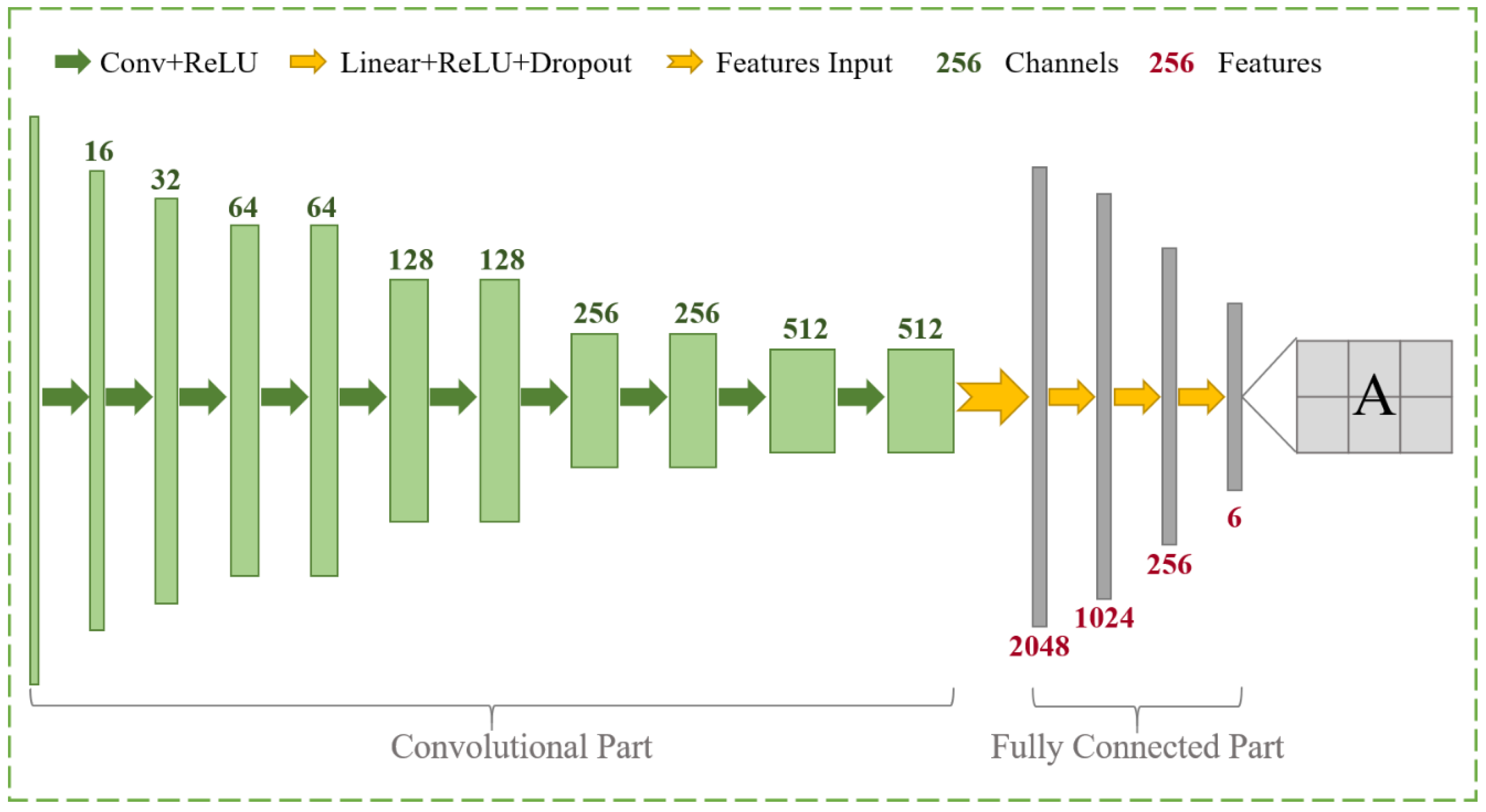
3.1.1. The Coarse Alignment Using the ARM

Generally, the deformation between two real remote sensing images is unpredictable, especially in mountainous regions, which cannot be well registered by the common scheme. To this end, the coarse-to-fine registration framework is always effective [7,25,26], and we enforced it based on CNN. The coarse registration using the ARM eliminates the relatively large deformations, such as the rotation and translation, which is equivalent to the traditional global alignment method using the area-based or feature-based approaches.

As illustrated in Figure 4, the convolution part is employed to gradually downsample the input feature maps and capture the high-level semantic features. The fully connected (FC) layers regress the affine transformation matrix. The ten convolutional layers consist of the convolution parts, and each layer is followed by a nonlinear activation function of the rectified linear unit (ReLU) [52]. Unlike the general setting, the convolution stride equals two at the different scales in this paper, instead of the pooling layers used to reduce the size of the feature map by half [53]. With the reduction in the image scale, the number of feature channels containing high-level semantic information gradually increases. Subsequently, the learned features are delivered to the FC part, consisting of four layers. In the first three layers, the input features are successively linearized to the specified ReLU and dropout function [54]. It is worth noting that the dropout function can randomly delete some nodes in the training stage, avoiding overfitting, especially for a complex network with a small dataset [55]. The last FC only contains the linear layer used to transform the previous features into six parameters for further regression of the transformation model. The six output numeric parameters represent a $2\times 2$ transform matrix and a $2\times 1$ translation matrix. Concretely, the former depicts the rotation, scaling, or shearing transformation, and the last one is the translation vector of the x- and y-directions. With the regressed transformation matrix A, the pixel-by-pixel displacement field is defined as:

$$D{F}_A:\{\begin{array}{l}\Delta x=a_{0}x+a_{1}y+a_2-x\\ \Delta y=a_{3}x+a_{4}y+a_5-y\end{array}$$

(1)

where $(x,y)$ represents the specified coordinate in the sensed image and $A=\left[\begin{array}{ccc}{a}_0& a_1& a_2\\ a_3& a_4& a_5\end{array}\right]$ is the affine transformation model. The sensed image is then transformed in accordance with the displacement field and resampled by the bilinear interpolation, obtaining the coarsely aligned image.

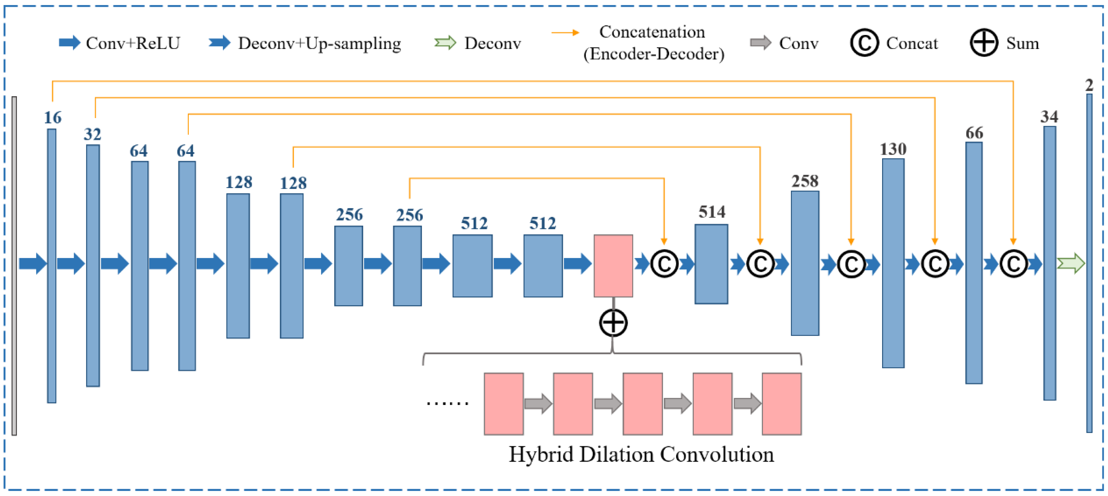
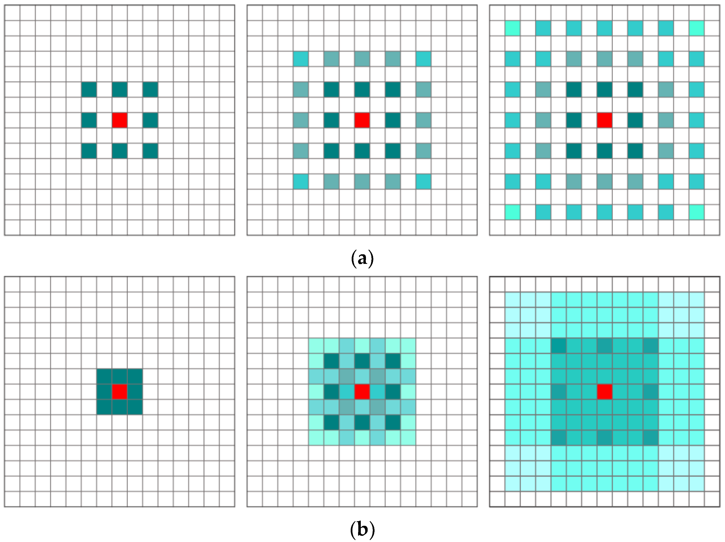
3.1.2. The Refinement Registration Network with the HDCED

Despite the performance of the ARM for reducing large and global deformations, the very local and varied distortions still remain in the reference and sensed image. To further eliminate them to achieve fine alignment, the refinement registration network of the HDCED is constructed following the ARM.

The encoder network is the same as the convolutional part of the ARM, which involves downscaling the input feature image gradually and capturing the high-level semantic information. The decoder network is designed to upscale the input feature maps and recover the spatial information progressively. It consists of six layers and is symmetrical to the encoder network. The deconvolutional layers are learned to expand the input size and reduce the number of input feature channels. Therefore, each deconvolutional layer contains elements from three aspects, including the deconvoluted feature maps, the upsampled one, and the feature maps from the encoder subnetwork of the same scale, which is the skip connection, as we know. The channels of the feature map are labeled on the head of each layer at the encoder and decoder stages, as shown in Figure 5. The submodule will output the per-pixel displacement field, using a feature map with two channels (displacement for the x- and y-directions) of the same size as the input. Especially the pink part is prominent, consisting of five stacked HDC blocks.

Dilated convolutions are important for image processing tasks, as they enlarge the receptive fields of the network without downsampling or increasing the number of model parameters [56], as shown in Figure 6a. However, the gridding effect is apparent with increasing dilation rates, expanding the receptive fields of output neurons [57]. Moreover, using large dilation rate information may only be beneficial for some large regions, and it may demonstrate disadvantages for small objects and may miss some detailed information [56]. To make full use of the image information, borrowing the idea in [58], we adopted an HDC block in the encoder–decoder network. The HDC utilizes the general convolution operation to further learn the abstract features in detail, as shown in Figure 6b. Although the operation principle is the same, the dilation rate of the HDC is not invariable. The dilation rate in this paper consists of five subsequent convolutional layers with dilation rates of 1, 3, 5, 7, and 11, respectively.

3.2. Implementation Details of the Proposed Framework

In the proposed network, the kernel size of all convolutional layers is $3\times 3$, while it is $4\times 4$ in the decoder network, and these kernels are initialized randomly from a Gaussian distribution. The Adam solver is utilized to optimize the entire network [59]. The network is trained for 100 epochs, and the learning rate is initialized to 0.001 and then decreased by a factor of 0.96 every ten epochs. All experiments are conducted in a workstation with a Pytorch neural network architecture and an NVIDIA GeForce GTX 3080 GPU.

Theoretically, the proposed framework is unsupervised, whereby the real deformation between the reference and sensed image is unknown. Our primary aim here is to learn the relative position of the sensed image compared to the reference one. Under this circumstance, the reference image is the golden standard and the warped image should have the same spatial position as far as possible. We introduce the correlation coefficient as the similarity measurement to evaluate the registration result, defined as follows:

$$CorrCoef[I_r,I_s]=\frac{Cov[I_r,I_s]}{\sqrt{Cov[I_r,I_r]}\sqrt{Cov[I_s,I_s]}}$$

(2)

where $Cov$ represents the covariance. The covariance between $I_r$ and $I_s$ is defined as:

$$Cov[I_r,I_s]=\frac{1}{M\times N}{\displaystyle \sum _{i=1}^M{\displaystyle \sum _{j=1}^N(I_r(i,j)-{\mu }_r)(I_s(i,j)-{\mu }_s)}}$$

(3)

$M\times N$ points to the image size, and the reference image has the same size as the sensed image; ${\mu }_r$ and ${\mu }_s$ are the means of the image intensity of the reference and sensed images, respectively.

Additionally, regularization losses are introduced to prevent the displacement field from being unrealistic or overfitting. They are constructed with the first-order gradient of a two-channel displacement field.

$$RL=\frac{1}{M\times N}{\displaystyle \sum _{i=1}^M{\displaystyle \sum _{j=1}^N{(\nabla u(i,j))}^2+{(\nabla v(i,j))}^2}}$$

(4)

where $u$ and $v$ are the displacement field in the $x$- and $y$-directions; $\nabla$ represents the gradient of the specified variable.

Therefore, the loss function of the proposed network framework is defined as:

$$Loss=CorrCoef+RL$$

(5)

To derive the appropriate and accurate registration result, we execute the refinement registration with the HDCED iteratively. The previous output is connected with the reference image in the channel dimension and fed into the current operation. Theoretically, the more times the loop is conducted, the better the registration result will be. Then, we set five iterations in our enforcement process to balance the accuracy of the alignment and running time. The final aligned and reference images are employed to calculate the similarity, further adjusting the network parameters for outperformance.

4. Experiments

First, the testing set of the MID is quantitatively and qualitatively analyzed to evaluate the registration performance of the proposed pipeline, as well as some typical approaches. Firstly, the evaluation indicators and the experimental scheme are described in Section 4.1. Then, Section 4.2 presents a detailed comparison of the proposed alignment scheme, including the visual comparisons and the quantitative evaluation between the coarse registration using the ARM and the result of the ARM together with the five iterated HDCED phases. Section 4.3 describes the performance comparison with the latest technologies based on the MID, including SIFT [21], a registration method used for building the local models by blocking (APAP) [60], an unsupervised multistep deformable registration (UMDR) approach [45], and a registration algorithm based on improved optical flow estimation (OFM) [11].

4.1. Evaluation Metrics and Experimental Scheme

The visual observation of the reference and aligned images using swipe view is intuitive and accurate, although it is a bit subjective and depends on personal experience. Thus, quantitative indicators are employed, assisting each other to fully evaluate the alignment using three indicators: the MI [7], structural similarity (SSIM), and root means square error (RMSE) [25,61,62].

The MI is a radiation-related indicator directly calculated from the intensity information. It is generally employed as the similarity index of the intermediate process of area-based registration. We take advantage of the MI to estimate the overall alignment, which is defined as:

$$MI(R,S)=H(R)+H(S)-H(R,S)$$

(6)

where $H(R)$ and $H(S)$ are the entropies of the reference and sensed images, respectively, and $H(R,S)$ is the joint entropy. The similarity between the two images grows as the MI increases, i.e., the registration result gradually gets better.

The development in the mountainous region is relatively slower than in the flat region, and the structure of the corresponding image changes little over time. Therefore, we employ the SSIM as an additional similarity measurement to judge the alignments [63,64]. It is defined as:

$$SSIM[I_r,I_s]=\frac{(2{\mu }_r{\mu }_s+c_1)(2{\sigma }_{rs}+c_2)}{({\mu }_r^2+{\mu }_s^2+c_1)({\sigma }_r^2+{\sigma }_s^2)}$$

(7)

where ${\mu }_r$ and ${\mu }_s$ are the averages of the corresponding image intensity levels, and ${\sigma }_x$ and ${\sigma }_y$ are the variance levels; ${\sigma }_{rs}$ represents the covariance between the reference and warped images; $c_1={(k_{1}L)}^2$, $k_1=0.01$, and $L$ represents the range of image intensity levels; $c_2={(k_{2}L)}^2$ and $k_2=0.03$.

Generally, there should be the same ground object on the same coordinate for two aligned images, i.e., the Euclidean distance of the corresponding surface features should be zero. Therefore, many pairs of coordinates are manually selected to calculate the mean distance, i.e., the RMSE, to quantitatively evaluate the alignment:

$$RMSE=\sqrt{\frac{1}{N}{\displaystyle \sum _{i=1}^N{(\Delta x_i)}^2+{(\Delta y_i)}^2}}$$

(8)

where $N$ is the number of points. $\Delta x_i$ and $\Delta y_i$ are the residual differences of the $i-th$ checkpoint pair in the $x$- and $y$-directions respectively. A smaller RMSE means a better result. For the RMSE calculation, several evaluated points were manually extracted from the reference and aligned images.

It is known that the SIFT aims to extract feature points for transformation model estimation, and the global matrix is representative of the classic approach [21]. The core of the APAP approach is blocking, whereby images are divided into many blocks and each of them owns a mapping function [60]. Perhaps it will perform well in mountainous remote sensing image registration, as the local deformation can be considered. The OFM allowing for the varied distortions calculates the pixel-by-pixel displacement for the corresponding coordinates of the two images. Additionally, it corrects the abnormal displacement caused by the LULC [12] with some predefined parameters. The UMDR based on a network is employed in [45], which is similar to our proposed algorithm, which adopts the iterative registration without the coarse alignment using the ARM. Moreover, the maximum displacement is assessed and specified in advance, which may influence the registration result with an inappropriate initial value.

Since there are many images used for testing, some registration results are displayed for visual observation. For example, there are four aligned images used for the internal comparison of our proposed algorithm in the ablation experiment, and four are used for a comparison of the different registration methods.

4.2. Ablation Experiment for the Proposed Algorithm

As presented in Section 3, the proposed algorithm generally consists of two parts, the ARM and HDCED. The ARM appears in the preregistration stage, and the HDCED is designed to refine the previous result. In other words, the ARM provides an initial reduction in deformation between the reference and sensed images, as shown in Figure 7. When simultaneously overlapping the reference and sensed images of each pair, the generated images are indefinable, and many ghosts are found in the significant ridgelines or valleys. These effects are mitigated in the preregistration results in Figure 7d, as aligned by the ARM. Fortunately, the overlapping of the results from the entire proposed algorithm and the reference image is clear, which looks like a whole image, as presented in the fifth column of Figure 7. To further observe the results, some subimages are selected and enlarged in Figure 8. While observing the enlarged subimages, we came to the same conclusion. There are large deformations of two mountainous remote sensing images when focusing on the seams in the vertical and horizontal directions. Most of the deformation is largely eliminated by the ARM, which provides an ideal input for the subsequent alignment. After five iterations of the HDCED, the high-precision alignments are generated, as shown in Figure 8c,f. Both in the horizontal and vertical directions, ignoring a seam line in the middle of the image, the mosaicked subimage looks like a complete one, where the connected linear features are not misplaced.

Additionally, we conducted a quantitative analysis to make the internal comparison more reliable. The MI and SSIM indicators were adopted as the accuracy metrics to respectively evaluate the alignment regarding the intensity consistency and structure consistency aspects. The higher the values of the MI and SSIM, the better the registration performance. As shown in

Table 2. Internal quantitative comparison of the proposed algorithm.

Experiment	Indicators	Original	ARM	Proposed
Test-1	MI (↑)	0.2650	1.0730	1.2459
	SSIM (↑)	0.1735	0.1880	0.9115
Test-2	MI (↑)	0.2428	0.9370	1.0843
	SSIM (↑)	0.1175	0.2273	0.8592
Test-3	MI (↑)	0.1712	0.6416	0.7277
	SSIM (↑)	0.1676	0.6846	0.8490
Test-4	MI (↑)	0.0779	0.4422	0.5515
	SSIM (↑)	0.1591	0.2914	0.7690

, all values are maximized in the proposed method column, demonstrating that refining the preregistered result using the HDCED iteratively is necessary. Additionally, the ARM is indispensable for decreasing the large deformation between the reference and sensed images and delivers the preregistered results to the refinement stage for more accurate outputs.

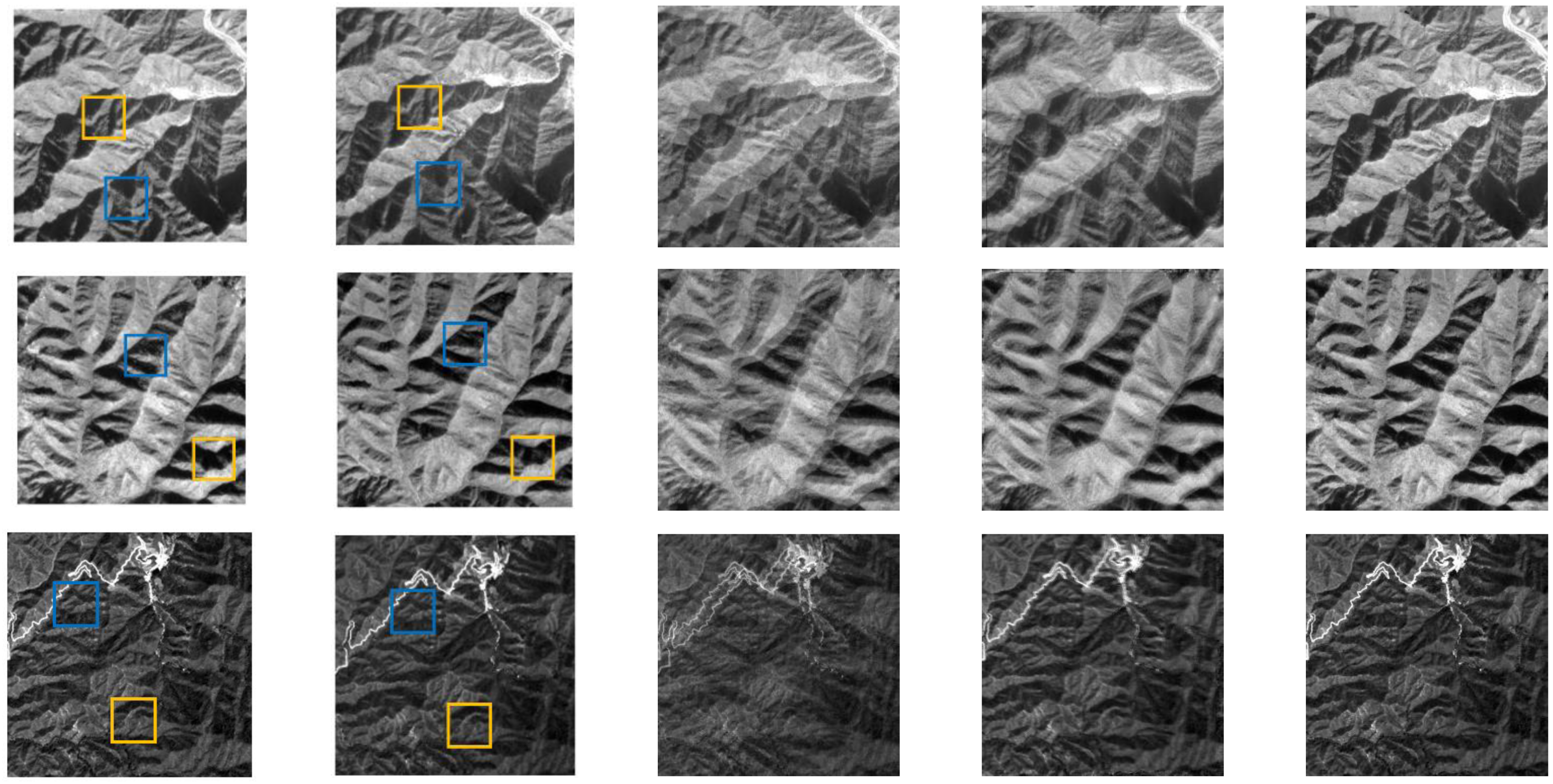
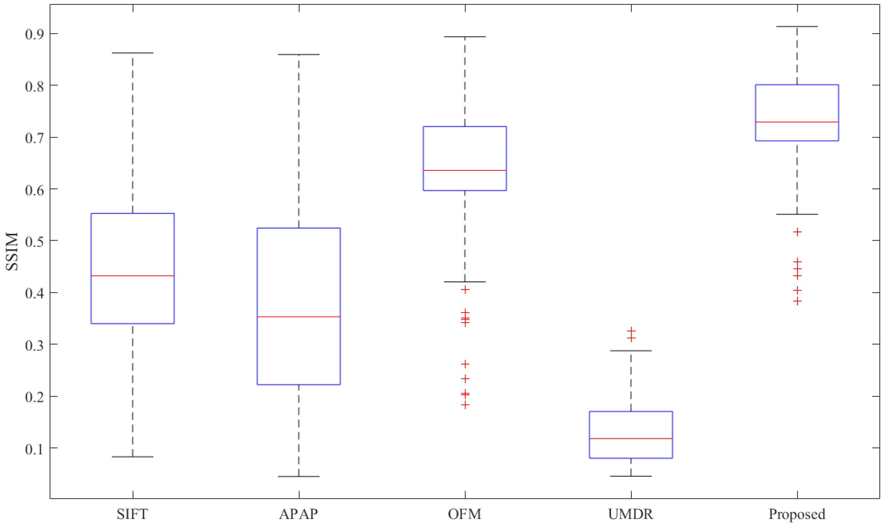
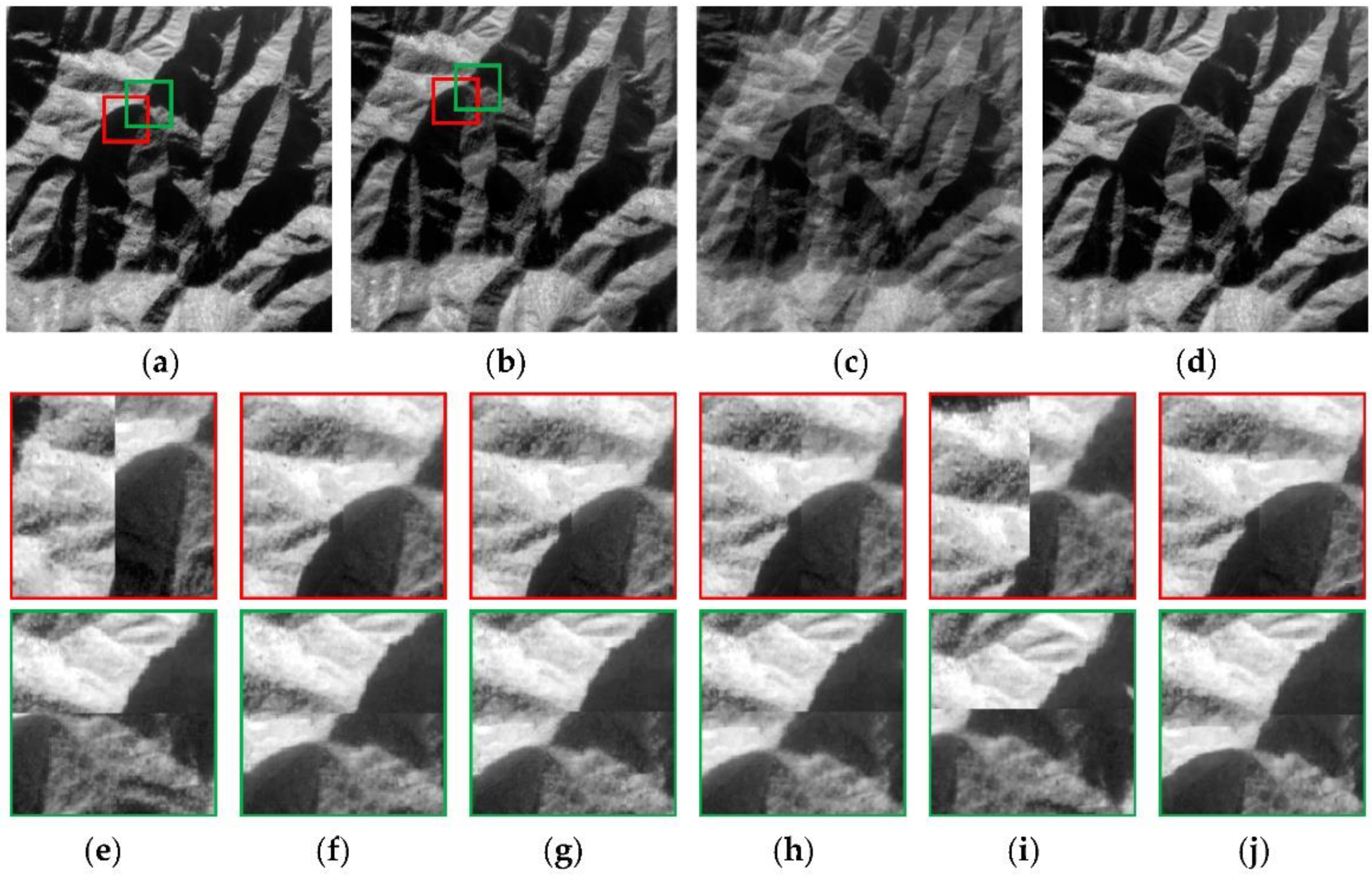
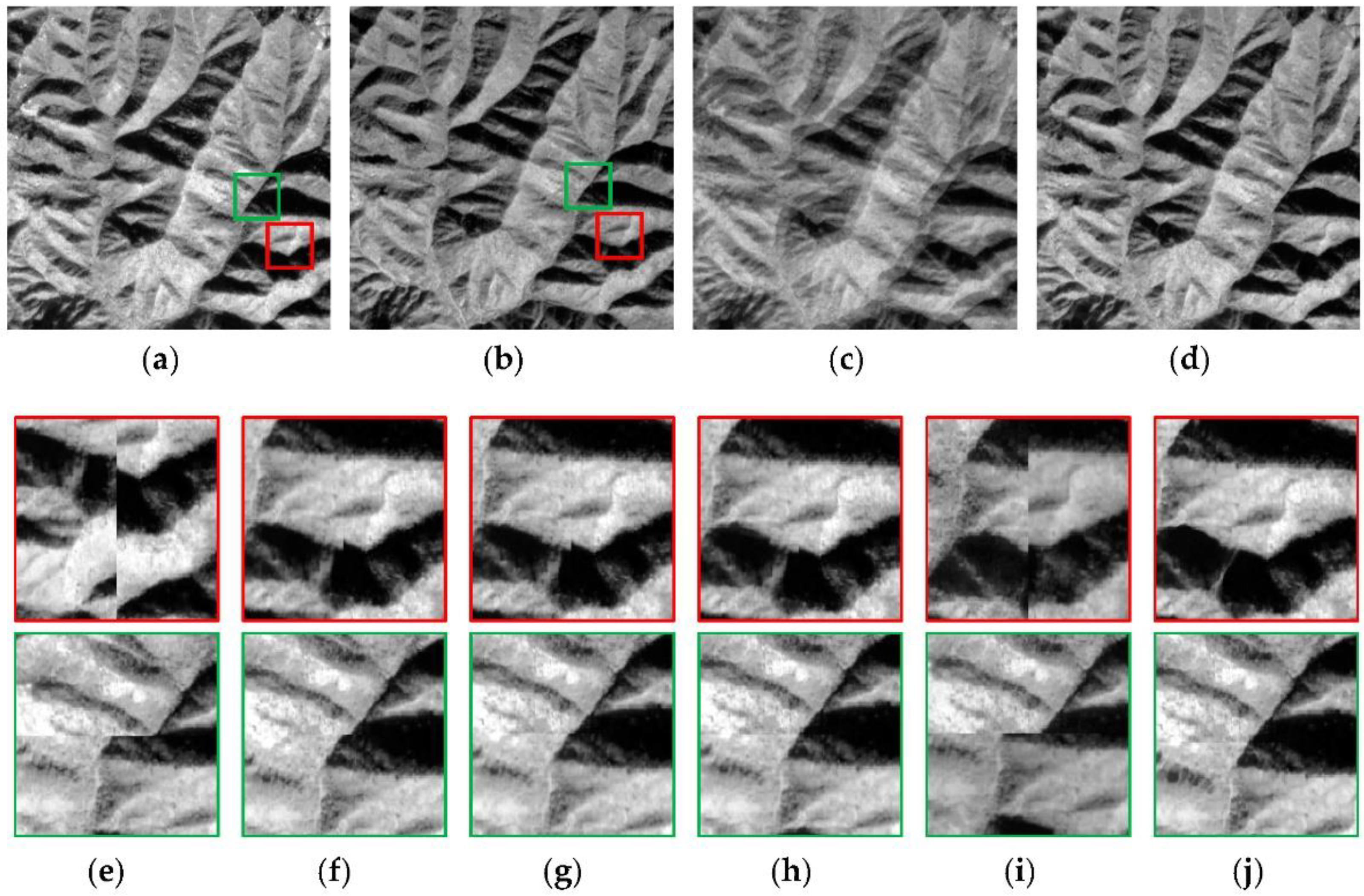
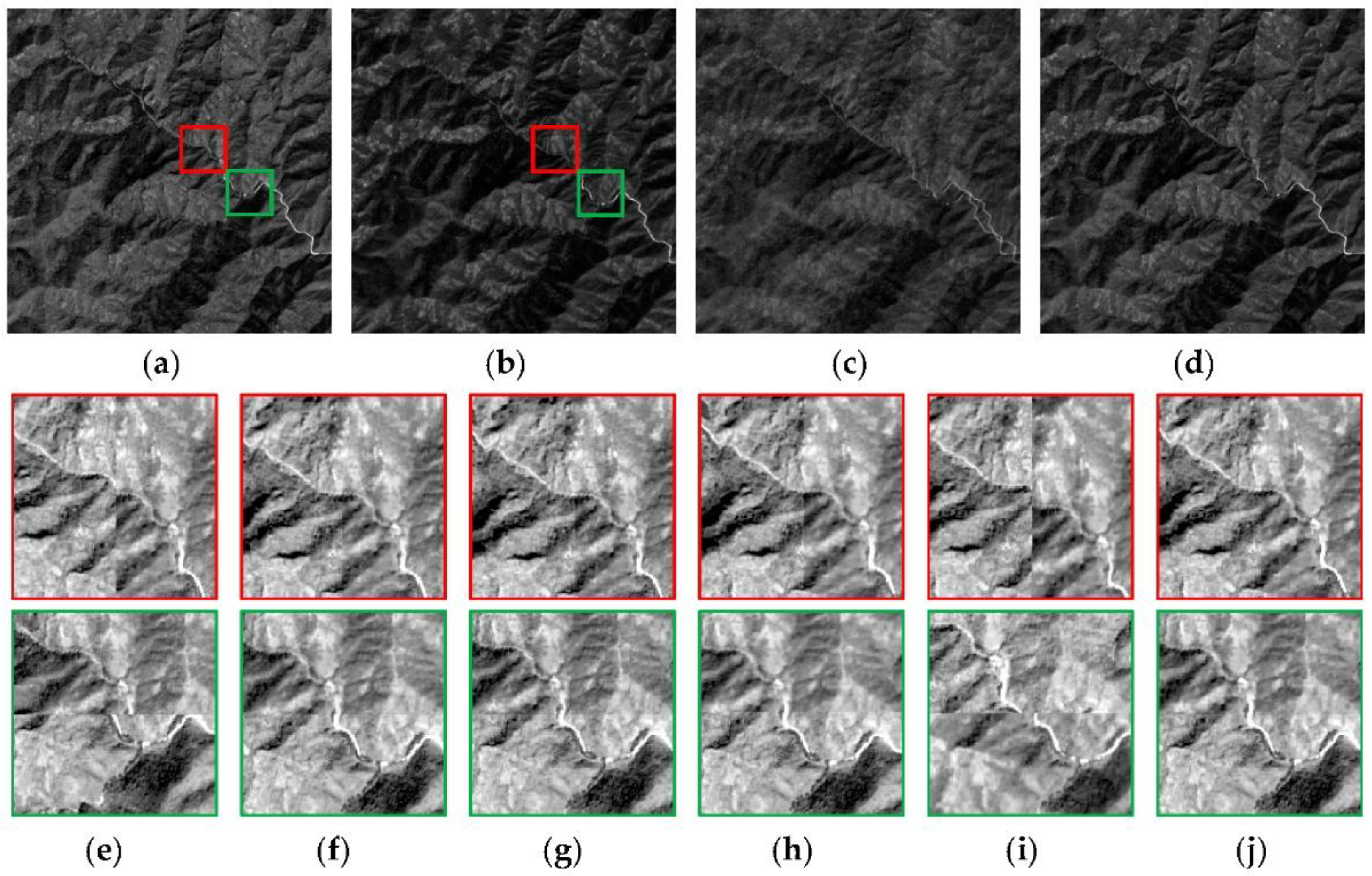
4.3. Comparison between the Proposed and Other Algorithms

The above qualitative and quantitative analysis shows that the proposed registration strategy successively solves the mountainous remote sensing image registration problem. To further demonstrate the proposed algorithm, we compare it with four different approaches that are representative of conventional or deep-learning-based methods. The SSIM indicator is adopted as the accuracy metric, and the higher the SSIM, the better the registration performance. Furthermore, to verify the robustness of the proposed algorithm, we introduce the box plot to show the SSIM. The advantage of the box plot is that it can accurately and stably present the SSIM distribution without being affected by outliers, and is particularly useful for comparing distributions between several sets of data. The box plot is based on a five-number summary: the minimum, first quartile, median, third quartile, and maximum. The box size is decided by the region between the first and third quartiles of the SSIM distribution. If the box is too large, the SSIM distribution is discrete with fluctuation, and on the contrary the data are concentrated. On the other hand, the spaces between the minimum and first quartile and between the third quartile and maximum can also indicate the degree of dispersion in the data, i.e., the smaller the space, the more concentrated the data [65].

As shown in Figure 9, the box plots record the SSIM distributions of the compared methods for 467 pairs of mountainous remote sensing images in our testing dataset. It can be seen that the box size and space between the minimum and first quartile and between the third quartile and maximum for the proposed algorithm are the smallest. Moreover, the box location of the proposed algorithm is the highest as well, demonstrating the robustness and superiority of the proposed method.

As presented in Section 4.2, the visual comparison can provide the observer with direct discovery in detail to ensure a quantitative evaluation for a comprehensive comparison. Therefore, four representative testing images with inconsistent surface structural features are selected, as shown in Figure 10, Figure 11, Figure 12 and Figure 13. The original reference and sensed images are listed in Figure 10a,b, Figure 11a,b, Figure 12a,b and Figure 13a,b, respectively. When overlapping, as shown in Figure 10c, Figure 11c, Figure 12c and Figure 13c, unsurprisingly there are distinct ghosts, and it can be seen that the image comes from two different ones. This is because the two images to be registered are not in the same coordinate system, and the same ground surface features have different spatial positions. Subsequently, when putting the focus on Figure 10d, Figure 11d, Figure 12d and Figure 13d, the overlapping images are the combination of the reference image and the aligned result from the proposed algorithm. The ridges and valleys are clear enough, and a few buildings are well defined also. Most importantly, the overlaid image looks like a single image rather than the superposition of two different ones.

Since comparisons of the registration effects of different algorithms based on the blur degree of the overlapping images are limited, some subimages from the swipe views of the reference and aligned images were extracted and enlarged, as shown in Figure 10f–j, Figure 11f–j, Figure 12f–j and Figure 13f–j. To effectively observe the registration result, the concentration should be placed on the seams of the subimage. Figure 10e, Figure 11e, Figure 12e and Figure 13e show that large and significant deformations can be found between the original reference and sensed images. Therefore, the overlapping images in Figure 10c, Figure 11c, Figure 12c and Figure 13c are blurry. For the traditional methods, the SIFT method can eliminate most of the deformation, but the linear features are still staggered at the edges in the horizontal and vertical directions, as the subimages in Figure 10f, Figure 11f, Figure 12f and Figure 13f show. The reason for this is that the SIFT algorithm only represents the feature point detection and extraction processes, and is popular and robust in the computer vision and remote sensing fields. It may not perform well with the weak textures of mountainous remote sensing images, and some mismatched feature points may be found for the repeated textures. Moreover, the global transformation model could not accurately describe the local spatial position mapping. Additionally, the APAP approach is based on the SIFT as well, whereby the local transformation models are applied. Figure 10g, Figure 11g, Figure 12g and Figure 13g show that the geometric dislocations at the seams are further reduced by the APAP approach. Even in Figure 13g, the sensed image is completely aligned to the reference image in the vertical direction. The distortion in the horizontal direction is sufficiently small and almost invisible. The sensed images of the OFM in Figure 10h and Figure 12h are completely registered to the reference in the horizontal direction, and the very high-precision registration appears in Figure 13h. The misalignment of the remaining subimages is caused by the inaccurate displacements from the OFM. The OFM mainly constructs a variational model with grayscale and gradient consistency as the constraint conditions. When the image content is inconsistent due to the disunity of the imaging angles, the estimated displacements may be inaccurate, meaning they cannot be completely corrected by the OFM, successively causing misalignment. In addition, the OFM is sensitive to large deformation. Unfortunately, the UMDR approach generates the most terrible alignments of the four visual experiments and gives only a tiny improvement over the original reference and sensed images, as shown in Figure 10i, Figure 11i, Figure 12i and Figure 13i. This is because the rough maximum displacement of the trained data cannot be known in advance. The inappropriate initial value misleads the trained network, resulting in the unregistered image. Compared with the four approaches, the proposed algorithm accurately aligns the sensed image to the reference image in the horizontal and vertical directions, as shown in Figure 10j, Figure 11j, Figure 12j and Figure 13j. The linear features at the joint of the two views are sequential and look like they come from the same scene. Above all, the OFM shows suboptimal performance in mountainous remote sensing image registration. The alignments generated by the proposed method are more accurate where the spatial positions of the corresponding ground objects are almost identical.

Furthermore, some distinct points are simultaneously selected in the reference, sensed, and aligned images to calculate the RMSE values of the corresponding pixels to further compare the proposed algorithm with the other four registration methods quantitatively. As shown in

Table 3. The RMSE values of the above experiments (pixels).

	Original	SIFT	APAP	OFM	UMDR	Proposed
test 1	39.8819	2.8262	2.5981	3.5969	39.436	0.4099
test 2	39.0149	3.7366	2.0555	3.5231	32.5883	0.6124
test 3	20.9156	1.6163	1.5411	0.4330	19.4459	0.3708
test 4	26.0337	0.5000	1.9333	0.4743	25.5903	0.2739

, on the whole, the large deformations between the reference and sensed images are significantly reduced by the listed registration algorithms. The proposed algorithm achieves remarkable alignments in the four experiments because of the subpixel results for the mountainous remote sensing images. In the first and second experiments, the OFM produces a worse registration result than those of the SIFT and APAP approaches. When observing the experimental images, there is an obvious non-correspondence of the surface features in the reference and sensed images caused by the different imaging viewpoints. This leads to incorrect displacements and subsequently causes low registration. The calculated RMSE is large since we extracted some feature points at these locations, indicating that the OFM generates low registration accuracy in these experiments. For the last experiment, the APAP exhibits a high RMSE, which is not what we expected, as some inaccurate transformation models are given to the local image blocks. The registration accuracy of the UMDR is the worst among the methods, and its improvement is negligible compared with the original RMSE. Perhaps giving an appropriate maximum displacement is beneficial for a high-precision registration approach. However, the deformation of different remote sensing images cannot be known in advance.

5. Discussion

The number of iterations used for refinement registration using the HDCED determines whether the program ends or not. This is critical in all parameters of our program, and the number of iterations was set as five in the experiments. Here, some discussions will be presented for this parameter, and experiments regarding the specified number will be analyzed as well. Additionally, we plan to further discuss the limitations of the proposed algorithm.

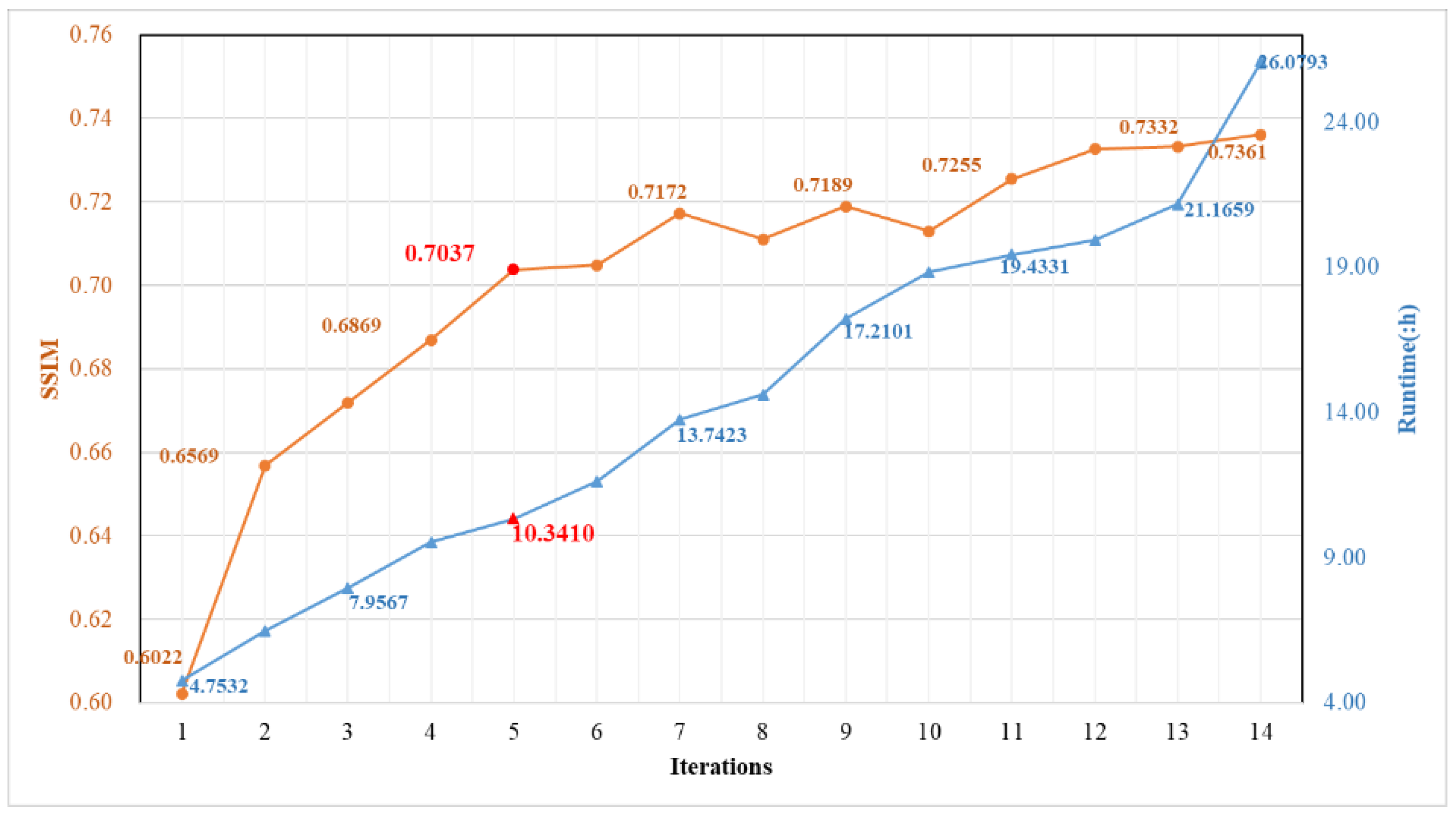
5.1. Definition of the Number of Iterations for Refinement Registration Using the HDCED

The geometric deformation process is complicated and variable between the reference and remote sensing images covering the mountainous region. The ARM is designed to eliminate the large and global deformations, without considering the local small distortions. The HDCED learns the high-level sematic features and regresses the per-pixel displacement field, focusing on the geometric relationship between each pair of corresponding pixels. Moreover, the HDCED could be executed for many iterations, progressively moving the displacement field as close to the perfect one as possible. However, the program cannot go on forever, leaving the ow to define the appropriate number of iterations, or when to stop the iterations?

Allowing for the memory of our GPU, we set the iteration numbers from one to fourteen. It is worth noting that the experimental configuration and parameters of each iteration were the same, except for the number of iterations. As described in Section 4, the structural similarity evaluation indicator (SSIM) was employed to evaluate the registration results. Since the training stage is generally time-consuming, it plays an essential role in evaluating an algorithm’s efficiency. The running times for the network training phases with different numbers of iterations were counted, as shown in Figure 14.

The SSIM values show a state of fluctuating growth as the iteration numbers of the HDCED increase, while the runtime shows a sustained increase. According to the trend of the orange line, the larger the iteration number, the better the registration result. However, the efficiency of the entire program and the performance of our workstation cannot be ignored. When the iteration number is 12, the increment of the runtime is minimal among all experiments, while there is just a 0.0072 increment in the SSIM. In other words, we did not obtain a more accurate alignment with a lower running time. Further, we compare the increment of the runtime and the SSIM values of two adjacent HDCED iterations. The number 5 gives a relatively favorable result. Concretely, when the iteration number increases to 5, the elapsed time increases by 0.8114 h and the SSIM grows by 0.0167. The increment of the runtime is relatively small, whereas the improvement of the aligned results is relatively large. Thus, we set 5 as the iteration number for the HDCED in our experiments.

5.2. Limitation

Generally, image registration processes are the prerequisites for image quality improvements, such as cloud removal, image stretching, and shadow removal processes. When we tested our proposed algorithm with a mountainous remote sensing image containing thin clouds, some abnormal contents appeared in the aligned image, as shown in Figure 15. The thin cloud or mist covers the reference image in Figure 15a, and the thickness of the cloud is not uniform. Conversely, the sensed image is relatively clear. No abundant geometric features can be found compared with the flat region images. The cloud or mist blurs the details of the image, aggravating the difficulty of the mountainous remote sensing image registration process. The calculated displacement field is not accurate enough, resulting in incorrectly transformed coordinates and subsequently causing abnormal contents, as shown in Figure 15c. This is against the basic principle of geometric registration. To overcome this disadvantage, we think that the image registration process should be conducted after the thin cloud or mist removal process. Additionally, we think that the SAR image covering the mountains is a good alternative without the influence of clouds, which is our next target. To comprehensively make use of their complementary information, we will achieve the accurate registration of SAR and optical images.

6. Conclusions

In this paper, we presented a novel mountainous remote sensing imagery dataset, consisting of 4093 pairs of image patches with the size of 512 × 512 pixels. It mainly covers a mountainous region, and is one of the few real remote sensing image registration datasets, which are rare in this field. Next, it will be expanded with more mountainous remote sensing images of other mountains in China for more research on the geometric registration process. Additionally, we developed an automatic image registration algorithm based on a coarse-to-fine unsupervised cascading convolutional network on the above dataset. The ARM was constructed to reduce the large deformations between the reference and sensed images, which generally cannot be predicted in advance. Then, the HDCED was used iteratively to successively eliminate the residual distortions, which were variable and very local. From the ablation experiments and the comparisons of the different registration algorithms, our proposed strategy provided high-precision alignments of the MID, preliminarily solving this challenging issue. Additionally, the availability of the new MID was verified, creating the possibility for the further development of unsupervised deep learning technologies for remote sensing image registration.

However, compared with the conventional registration algorithms, and even other deep learning-based methods, the proposed algorithm could only process remote sensing images of a specified size. In other words, when the model is trained with a large number of images measuring $512\times 512$ pixels, the test data should be of the same size. This greatly limits the popularization and application of this kind of algorithm. Perhaps the appropriate size of the images should be input to train the registration network, meeting the application requirements. The memory of the GPU and the computer performance must be improved. Furthermore, the larger images to be registered could be divided based on specified overlapping pixels, thereby inputting them into the training network. The final global displacement field can also be assembled by weighting the displacement fields of each local block. The problem will be further solved in future studies, as we hope the mountainous remote sensing image registration process can efficiently give accurate datasets for disaster detection and other mountainous research fields.

References

1. Jiang, X.; Ma, J.; Fan, A.; Xu, H.; Lin, G.; Lu, T.; Tian, X. Robust Feature Matching for Remote Sensing Image Registration via Linear Adaptive Filtering. IEEE Trans. Geosci. Remote Sens. 2020, 59, 1577–1591. [Google Scholar] [CrossRef]
2. Wu, Y.; Liu, J.-W.; Zhu, C.-Z.; Bai, Z.-F.; Miao, Q.-G.; Ma, W.-P.; Gong, M.-G. Computational Intelligence in Remote Sensing Image Registration: A survey. Int. J. Autom. Comput. 2020, 18, 1–17. [Google Scholar] [CrossRef]
3. Zitová, B.; Flusser, J. Image registration methods: A survey. Image Vis. Comput. 2003, 21, 977–1000. [Google Scholar] [CrossRef]
4. Feng, R.; Shen, H.; Bai, J.; Li, X. Advances and Opportunities in Remote Sensing Image Geometric Registration: A systematic review of state-of-the-art approaches and future research directions. IEEE Geosci. Remote Sens. Mag. 2021, 9, 120–142. [Google Scholar] [CrossRef]
5. Ye, Y.; Bruzzone, L.; Shan, J.; Bovolo, F.; Zhu, Q. Fast and Robust Matching for Multimodal Remote Sensing Image Registration. IEEE Trans. Geosci. Remote Sens. 2019, 57, 9059–9070. [Google Scholar] [CrossRef]
6. Ye, Y.; Shan, J.; Bruzzone, L.; Shen, L. Robust Registration of Multimodal Remote Sensing Images Based on Structural Similarity. IEEE Trans. Geosci. Remote Sens. 2017, 55, 2941–2958. [Google Scholar] [CrossRef]
7. Gong, M.; Zhao, S.; Jiao, L.; Tian, D.; Wang, S. A Novel Coarse-to-Fine Scheme for Automatic Image Registration Based on SIFT and Mutual Information. IEEE Trans. Geosci. Remote Sens. 2014, 52, 4328–4338. [Google Scholar] [CrossRef]
8. Yan, H.; Yang, S.; Xue, Q.; Zhang, N. HR optical and SAR image registration using uniform optimized feature and extend phase congruency. Int. J. Remote Sens. 2021, 43, 52–74. [Google Scholar] [CrossRef]
9. Brigot, G.; Colin-Koeniguer, E.; Plyer, A.; Janez, F. Adaptation and Evaluation of an Optical Flow Method Applied to Coregistration of Forest Remote Sensing Images. IEEE J. Sel. Top. Appl. Earth Obs. Remote Sens. 2016, 9, 2923–2939. [Google Scholar] [CrossRef]
10. Xiang, Y.; Wang, F.; Wan, L.; Jiao, N.; You, H. OS-Flow: A Robust Algorithm for Dense Optical and SAR Image Registration. IEEE Trans. Geosci. Remote Sens. 2019, 57, 6335–6354. [Google Scholar] [CrossRef]
11. Feng, R.; Du, Q.; Shen, H.; Li, X. Region-by-Region Registration Combining Feature-Based and Optical Flow Methods for Remote Sensing Images. Remote Sens. 2021, 13, 1475. [Google Scholar] [CrossRef]
12. Feng, R.; Du, Q.; Luo, H.; Shen, H.; Li, X.; Liu, B. A registration algorithm based on optical flow modification for multi-temporal remote sensing images covering the complex-terrain region. Natl. Remote Sens. Bull. 2021, 25, 630–640. [Google Scholar]
13. Plyer, A.; Colin-Koeniguer, E.; Weissgerber, F. A New Coregistration Algorithm for Recent Applications on Urban SAR Images. IEEE Geosci. Remote Sens. Lett. 2015, 12, 2198–2202. [Google Scholar] [CrossRef]
14. Paul, S.; Pati, U.C. A comprehensive review on remote sensing image registration. Int. J. Remote Sens. 2021, 42, 5396–5432. [Google Scholar] [CrossRef]
15. Zhang, X.; Wang, Y.; Liu, H. Robust Optical and SAR Image Registration Based on OS-SIFT and Cascaded Sample Consensus. IEEE Geosci. Remote Sens. Lett. 2021, 19, 1–5. [Google Scholar] [CrossRef]
16. Yang, W.; Wang, X.; Moran, B.; Wheaton, A.; Cooley, N. Efficient registration of optical and infrared images via modified Sobel edging for plant canopy temperature estimation. Comput. Electr. Eng. 2012, 38, 1213–1221. [Google Scholar] [CrossRef]
17. Palenichka, R.M.; Zaremba, M.B. Automatic Extraction of Control Points for the Registration of Optical Satellite and LiDAR Images. IEEE Trans. Geosci. Remote Sens. 2010, 48, 2864–2879. [Google Scholar] [CrossRef]
18. Kuppala, K.; Banda, S.; Barige, T.R. An overview of deep learning methods for image registration with focus on feature-based approaches. Int. J. Image Data Fusion 2020, 11, 113–135. [Google Scholar] [CrossRef]
19. Gang, H.; Yun, Z. Combination of feature-based and area-based image registration technique for high resolution remote sensing image. In Proceedings of the IEEE International Geoscience and Remote Sensing Symposium (IGARSS), Barcelona, Spain, 23–28 July 2007; pp. 377–380. [Google Scholar]
20. Zhang, P.; Luo, X.; Ma, Y.; Wang, C.; Wang, W.; Qian, X. Coarse-to-Fine Image Registration for Multi-Temporal High Resolution Remote Sensing Based on a Low-Rank Constraint. Remote Sens. 2022, 14, 573. [Google Scholar] [CrossRef]
21. Lowe, D.G. Distinctive Image Features from Scale-Invariant Keypoints. Int. J. Comput. Vis. 2004, 60, 91–110. [Google Scholar] [CrossRef]
22. Bay, H.; Ess, A.; Tuytelaars, T.; Van Gool, L. Speeded-Up Robust Features (SURF). Comput. Vis. Image Underst. 2008, 110, 346–359. [Google Scholar] [CrossRef]
23. Rublee, E.; Rabaud, V.; Konolige, K.; Bradski, G. ORB: An efficient alternative to SIFT or SURF. In Proceedings of the International Conference on Computer Vision (ICCV), Barcelona, Spain, 6–13 November 2011; pp. 2564–2571. [Google Scholar]
24. Pallotta, L.; Giunta, G.; Clemente, C. Subpixel SAR Image Registration Through Parabolic Interpolation of the 2-D Cross Correlation. IEEE Trans. Geosci. Remote Sens. 2020, 58, 4132–4144. [Google Scholar] [CrossRef]
25. Feng, R.; Du, Q.; Li, X.; Shen, H. Robust registration for remote sensing images by combining and localizing feature- and area-based methods. ISPRS J. Photogramm. Remote Sens. 2019, 151, 15–26. [Google Scholar] [CrossRef]
26. Ye, Y.; Shan, J. A local descriptor based registration method for multispectral remote sensing images with non-linear intensity differences. ISPRS J. Photogramm. Remote Sens. 2014, 90, 83–95. [Google Scholar] [CrossRef]
27. Ma, L.; Liu, Y.; Zhang, X.; Ye, Y.; Yin, G.; Johnson, B.A. Deep learning in remote sensing applications: A meta-analysis and review. ISPRS J. Photogramm. Remote Sens. 2019, 152, 166–177. [Google Scholar] [CrossRef]
28. Merkle, N.; Auer, S.; Muller, R.; Reinartz, P. Exploring the Potential of Conditional Adversarial Networks for Optical and SAR Image Matching. IEEE J. Sel. Top. Appl. Earth Obs. Remote Sens. 2018, 11, 1811–1820. [Google Scholar] [CrossRef]
29. Hughes, L.H.; Schmitt, M.; Mou, L.; Wang, Y.; Zhu, X.X. Identifying Corresponding Patches in SAR and Optical Images With a Pseudo-Siamese CNN. IEEE Geosci. Remote Sens. Lett. 2018, 15, 784–788. [Google Scholar] [CrossRef]
30. Hoffmann, S.; Brust, C.-A.; Shadaydeh, M.; Denzler, J. Registration of High Resolution Sar and Optical Satellite Imagery Using Fully Convolutional Networks. In Proceedings of the IEEE International Geoscience and Remote Sensing Symposium (IGARSS), Yokohama, Japan, 28 July–2 August 2019; pp. 5152–5155. [Google Scholar] [CrossRef]
31. Quan, D.; Wang, S.; Ning, M.; Xiong, T.; Jiao, L. Using deep neural networks for synthetic aperture radar image registration. In Proceedings of the IEEE International Geoscience and Remote Sensing Symposium (IGARSS), Beijing, China, 10–15 July 2016; pp. 2799–2802. [Google Scholar] [CrossRef]
32. Ye, F.; Su, Y.; Xiao, H.; Zhao, X.; Min, W. Remote Sensing Image Registration Using Convolutional Neural Network Features. IEEE Geosci. Remote Sens. Lett. 2018, 15, 232–236. [Google Scholar] [CrossRef]
33. Ma, W.; Zhang, J.; Wu, Y.; Jiao, L.; Zhu, H.; Zhao, W. A Novel Two-Step Registration Method for Remote Sensing Images Based on Deep and Local Features. IEEE Trans. Geosci. Remote Sens. 2019, 57, 4834–4843. [Google Scholar] [CrossRef]
34. Zhang, H.; Ni, W.; Yan, W.; Xiang, D.; Wu, J.; Yang, X.; Bian, H. Registration of Multimodal Remote Sensing Image Based on Deep Fully Convolutional Neural Network. IEEE J. Sel. Top. Appl. Earth Obs. Remote Sens. 2019, 12, 3028–3042. [Google Scholar] [CrossRef]
35. Quan, D.; Wang, S.; Gu, Y.; Lei, R.; Yang, B.; Wei, S.; Hou, B.; Jiao, L. Deep Feature Correlation Learning for Multi-Modal Remote Sensing Image Registration. IEEE Trans. Geosci. Remote Sens. 2022, 60, 1–16. [Google Scholar] [CrossRef]
36. Han, X.; Leung, T.; Jia, Y.; Sukthankar, R.; Berg, A.C. Matchnet: Unifying feature and metric learning for patch-based matching. In Proceedings of the IEEE conference on computer vision and pattern recognition, Boston, MA, USA, 7–12 June 2015; pp. 3279–3286. [Google Scholar]
37. Quan, D.; Liang, X.; Wang, S.; Wei, S.; Li, Y.; Huyan, N.; Jiao, L. AFD-Net: Aggregated Feature Difference Learning for Cross-Spectral Image Patch Matching. In Proceedings of the IEEE/CVF International Conference on Computer Vision, Seoul, Korea, 27 October–2 November 2019. [Google Scholar] [CrossRef]
38. Wang, S.; Quan, D.; Liang, X.; Ning, M.; Guo, Y.; Jiao, L. A deep learning framework for remote sensing image registration. ISPRS J. Photogramm. Remote Sens. 2018, 145, 148–164. [Google Scholar] [CrossRef]
39. Li, L.; Han, L.; Ding, M.; Liu, Z.; Cao, H. Remote Sensing Image Registration Based on Deep Learning Regression Model. IEEE Geosci. Remote Sens. Lett. 2020, 19, 8002905. [Google Scholar] [CrossRef]
40. Li, L.; Han, L.; Ding, M.; Cao, H.; Hu, H. A deep learning semantic template matching framework for remote sensing image registration. ISPRS J. Photogramm. Remote Sens. 2021, 181, 205–217. [Google Scholar] [CrossRef]
41. Haskins, G.; Kruger, U.; Yan, P. Deep learning in medical image registration: A survey. Mach. Vis. Appl. 2020, 31, 8. [Google Scholar] [CrossRef]
42. Zampieri, A.; Charpiat, G.; Girard, N.; Tarabalka, Y. Multimodal Image Alignment Through a Multiscale Chain of Neural Networks with Application to Remote Sensing. In Proceedings of the European Conference on Computer Vision (ECCV), Munich, Germany, 8–14 September 2018; pp. 679–696. [Google Scholar] [CrossRef]
43. DeTone, D.; Malisiewicz, T.; Rabinovich, A. Deep image homography estimation. arXiv 2016, arXiv:1606.03798. [Google Scholar]
44. Huang, G.; Liu, Z.; van der Maaten, L.; Weinberger, K.Q. Densely connected convolutional networks. In Proceedings of the IEEE Conference on Computer Vision and Pattern Recognition (CVPR), Honolulu, HI, USA, 21–26 July 2017; pp. 4700–4708. [Google Scholar]
45. Papadomanolaki, M.; Christodoulidis, S.; Karantzalos, K.; Vakalopoulou, M. Unsupervised Multistep Deformable Registration of Remote Sensing Imagery Based on Deep Learning. Remote Sens. 2021, 13, 1294. [Google Scholar] [CrossRef]
46. Balakrishnan, G.; Zhao, A.; Sabuncu, M.R.; Guttag, J.; Dalca, A.V. VoxelMorph: A Learning Framework for Deformable Medical Image Registration. IEEE Trans. Med. Imaging 2019, 38, 1788–1800. [Google Scholar] [CrossRef] [Green Version]
47. Stergios, C.; Mihir, S.; Maria, V.; Guillaume, C.; Marie-Pierre, R.; Stavroula, M.; Nikos, P. Linear and Deformable Image Registration with 3D Convolutional Neural Networks. In Image Analysis for Moving Organ, Breast, and Thoracic Images; Springer: Cham, Switzerland, 2018; pp. 13–22. [Google Scholar] [CrossRef]
48. Vakalopoulou, M.; Christodoulidis, S.; Sahasrabudhe, M.; Mougiakakou, S.; Paragios, N. Image Registration of Satellite Imagery with Deep Convolutional Neural Networks. In Proceedings of the IEEE International Geoscience and Remote Sensing Symposium (IGARSS), Yokohama, Japan, 28 July–2 August 2019; pp. 4939–4942. [Google Scholar] [CrossRef]
49. Zhao, S.; Dong, Y.; Chang, E.I.; Xu, Y. Recursive cascaded networks for unsupervised medical image registration. In Proceedings of the IEEE/CVF International Conference on Computer Vision, Seoul, Korea, 27–28 October 2019; pp. 10600–10610. [Google Scholar]
50. Zhao, S.; Lau, T.; Luo, J.; Chang, E.I.-C.; Xu, Y. Unsupervised 3D End-to-End Medical Image Registration With Volume Tweening Network. IEEE J. Biomed. Health Inform. 2019, 24, 1394–1404. [Google Scholar] [CrossRef]
51. Tian, B.; Li, Z.; Zhang, M.; Huang, L.; Qiu, Y.; Li, Z.; Tang, P. Mapping Thermokarst Lakes on the Qinghai–Tibet Plateau Using Nonlocal Active Contours in Chinese GaoFen-2 Multispectral Imagery. IEEE J. Sel. Top. Appl. Earth Obs. Remote Sens. 2017, 10, 1–14. [Google Scholar] [CrossRef]
52. Nair, V.; Hinton, G.E. Rectified linear units improve restricted boltzmann machines. In Proceedings of the 27th International Conference on International Conference on Machine Learning, Haifa, Israel, 21–24 June 2010. [Google Scholar]
53. Springenberg, J.T.; Dosovitskiy, A.; Brox, T.; Riedmiller, M. Striving for simplicity: The all convolutional net. arXiv 2014, arXiv:1412.6806. [Google Scholar]
54. Hinton, G.E.; Srivastava, N.; Krizhevsky, A.; Sutskever, I.; Salakhutdinov, R.R. Improving neural networks by preventing co-adaptation of feature detectors. arXiv 2012, arXiv:1207.0580. [Google Scholar]
55. Li, X.; Chen, S.; Hu, X.; Yang, J. Understanding the Disharmony Between Dropout and Batch Normalization by Variance Shift. In Proceedings of the IEEE/CVF Conf. on Computer Vision and Pattern Recognition (CVPR), Long Beach, CA, USA, 15–20 June 2019; pp. 2677–2685. [Google Scholar] [CrossRef]
56. Fang, Y.; Li, Y.; Tu, X.; Tan, T.; Wang, X. Face completion with Hybrid Dilated Convolution. Signal Process. Image Commun. 2019, 80, 115664. [Google Scholar] [CrossRef]
57. Iizuka, S.; Simo-Serra, E.; Ishikawa, H. Globally and locally consistent image completion. ACM Trans. Graph. 2017, 36, 107. [Google Scholar] [CrossRef]
58. Wang, P.; Chen, P.; Yuan, Y.; Liu, D.; Huang, Z.; Hou, X.; Cottrell, G. Understanding Convolution for Semantic Segmentation. In Proceedings of the 2018 IEEE Winter Conference on Applications of Computer Vision (WACV), Lake Tahoe, NV, USA, 12–15 March 2018; pp. 1451–1460. [Google Scholar]
59. Kingma, D.P.; Ba, J. Adam: A method for stochastic optimization. arXiv 2014, arXiv:1412.6980. [Google Scholar]
60. Zaragoza, J.; Chin, T.J.; Tran, Q.H.; Suter, D. As-Projective-As-Possible Image Stitching with Moving DLT. IEEE Trans. Pattern Anal. Mach. Intell. 2014, 36, 1285–1298. [Google Scholar]
61. Han, Y.; Bovolo, F.; Bruzzone, L. An Approach to Fine Coregistration Between Very High Resolution Multispectral Images Based on Registration Noise Distribution. IEEE Trans. Geosci. Remote Sens. 2015, 53, 6650–6662. [Google Scholar] [CrossRef]
62. Wong, A.; Clausi, D.A. ARRSI: Automatic Registration of Remote-Sensing Images. IEEE Trans. Geosci. Remote Sens. 2007, 45, 1483–1493. [Google Scholar] [CrossRef]
63. Zhao, H.; Gallo, O.; Frosio, I.; Kautz, J. Loss functions for neural networks for image processing. arXiv 2015, arXiv:1511.08861. [Google Scholar]
64. Wang, Z.; Bovik, A.; Sheikh, H.; Simoncelli, E. Image Quality Assessment: From Error Visibility to Structural Similarity. IEEE Trans. Image Process. 2004, 13, 600–612. [Google Scholar] [CrossRef] [Green Version]
65. Luo, S.; Li, H.; Shen, H. Deeply supervised convolutional neural network for shadow detection based on a novel aerial shadow imagery dataset. ISPRS J. Photogramm. Remote Sens. 2020, 167, 443–457. [Google Scholar] [CrossRef]
Figure 1. Image distribution of our MID.
Remotesensing 14 04178 g001
Figure 2. Overlapping extraction and clipping process for a pair of images.
Remotesensing 14 04178 g002
Figure 3. Overview of the proposed framework. (Note: For visual observation of the registration result, the brightness of the reference image in swipe view is adjusted; “n” is the number of iterations, and “N” is the predefined maximum number of iterations.)
Remotesensing 14 04178 g003
Figure 4. Structure of the affine registration network.
Remotesensing 14 04178 g004
Figure 5. Overview of the HDCED used for the refinement of the registration process.
Remotesensing 14 04178 g005
Figure 6. Illustration of the gridding problem. (a) All convolutional layers exhibit the same dilation rate r = 2. From left to right: Green marked features correspond to the calculation of the central red feature using three convolution layers with a 3 × 3 kernel size. (b) Subsequent convolutional layers exhibit dilation rates of r = 1, 2, and 3, respectively. This means the receptive field is unchanged without the gridding problem.
Remotesensing 14 04178 g006
Figure 7. Registration results for the ARM and the entire proposed framework. (a) The reference image, (b) the sensed image, (c) the overlap between the reference and sensed image, (d) the overlap between the reference and ARM aligned result, and (e) the overlap between the reference and proposed alignments. (Note: the sub-image surrounded by the blue and yellow rectangles will be enlarged and explained in the following.)
Remotesensing 14 04178 g007aRemotesensing 14 04178 g007b
Figure 8. Enlargement of selected subimages via the reference and sensed (aligned) image mosaic: (a) the original images, (b) the ARM result, and (c) the proposed result used for vertical observations; (d) the original images, (e) the ARM result, (f) and the proposed result used for horizontal observations.
Remotesensing 14 04178 g008
Figure 9. Box plots of SSIM distributions of different registration algorithms for 467 pairs of testing images. Note: the iteration number for the UMDR is three, as recommended, and the maximum displacement is set to ten when training the network with our training set, which may not be optimal.
Remotesensing 14 04178 g009
Figure 10. Visual comparisons of different registration methods used in test 1: (a) reference image; (b) sensed image; (c) overlap of the reference and the sensed images; (d) overlap of the reference and the proposed alignments. The enlarged subimages of (e) the original images, (f) SIFT, (g) APAP, (h) OFM, (i) UMDR, and (j) proposed image.
Remotesensing 14 04178 g010
Figure 11. Visual comparisons of different registration methods used in test 2: (a) reference image; (b) sensed image; (c) overlap of the reference and the sensed images; (d) overlap of the reference and the proposed alignments. The enlarged subimages of (e) the original images, (f) SIFT, (g) APAP, (h) OFM, (i) UMDR, and (j) proposed image.
Remotesensing 14 04178 g011
Figure 12. Visual comparisons of different registration methods used in test 3: (a) reference image; (b) sensed image; (c) overlap of the reference and the sensed images; (d) overlap of the reference and the proposed alignments. The enlarged subimages of (e) the original images, (f) SIFT, (g) APAP, (h) OFM, (i) UMDR, and (j) proposed image.
Remotesensing 14 04178 g012
Figure 13. Visual comparisons of different registration methods used in test 4: (a) reference image; (b) sensed image; (c) overlap of the reference and the sensed images; (d) overlap of the reference and the proposed alignments. The enlarged subimages of (e) the original images, (f) SIFT, (g) APAP, (h) OFM, (i) UMDR, and (j) proposed image.
Remotesensing 14 04178 g013
Figure 14. The SSIM and runtime results of the experiments with different iteration numbers for refinement registration using the HDCED.
Remotesensing 14 04178 g014
Figure 15. The registration of images obscured by thin clouds or mist: (a) reference image; (b) sensed image; (c) aligned image.
Remotesensing 14 04178 g015