
PIIE-DSA-Net for 3D Semantic Segmentation of Urban Indoor and Outdoor Datasets


Abstract
:
1. Introduction
2. Methodology
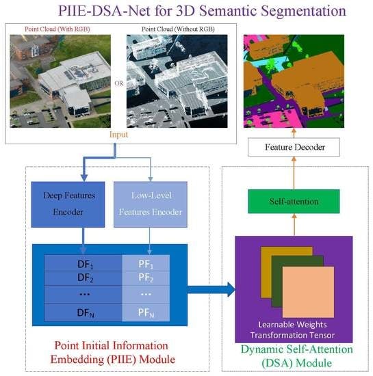
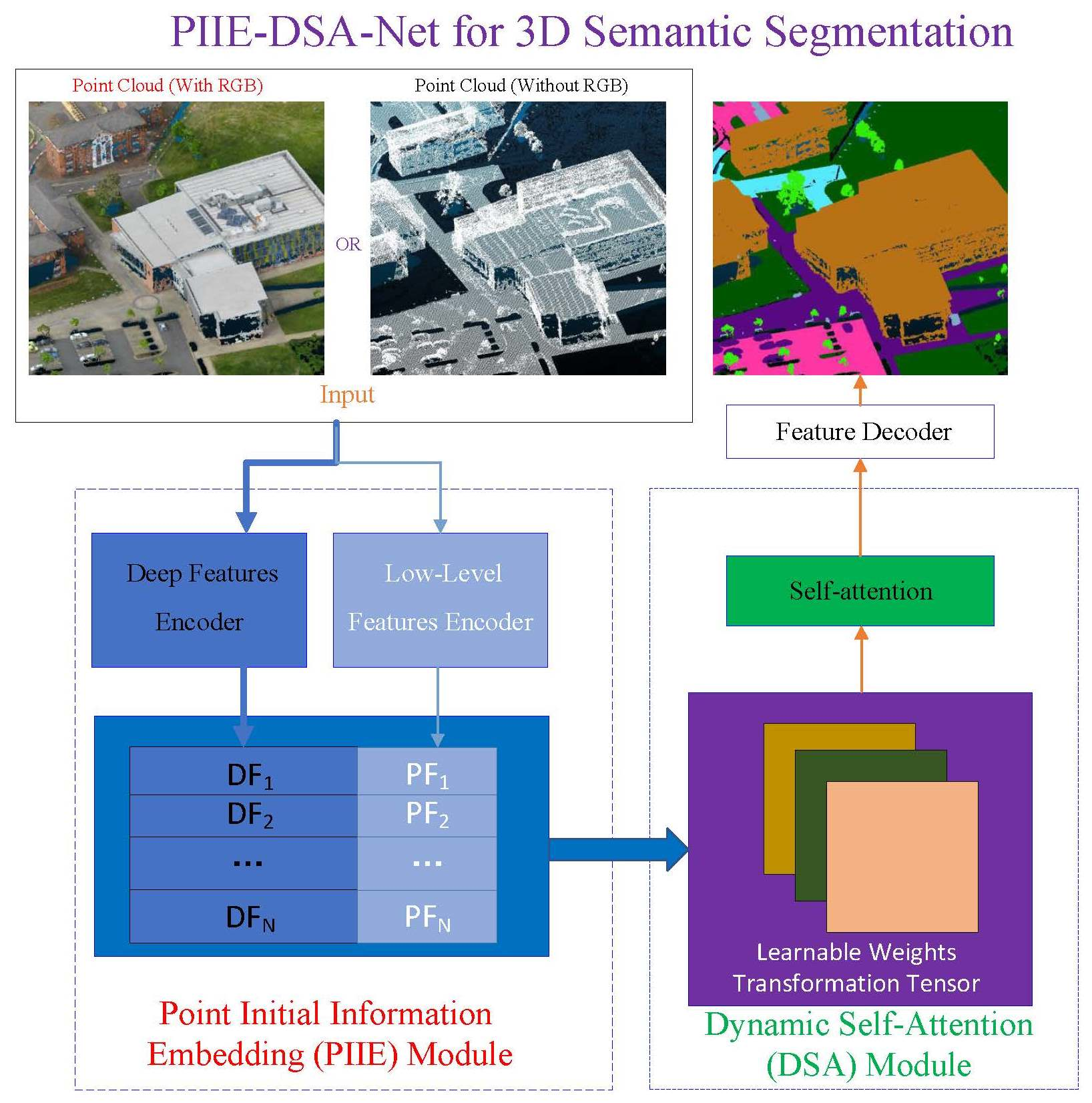
2.1. Framework of PIIE-DSA-Net
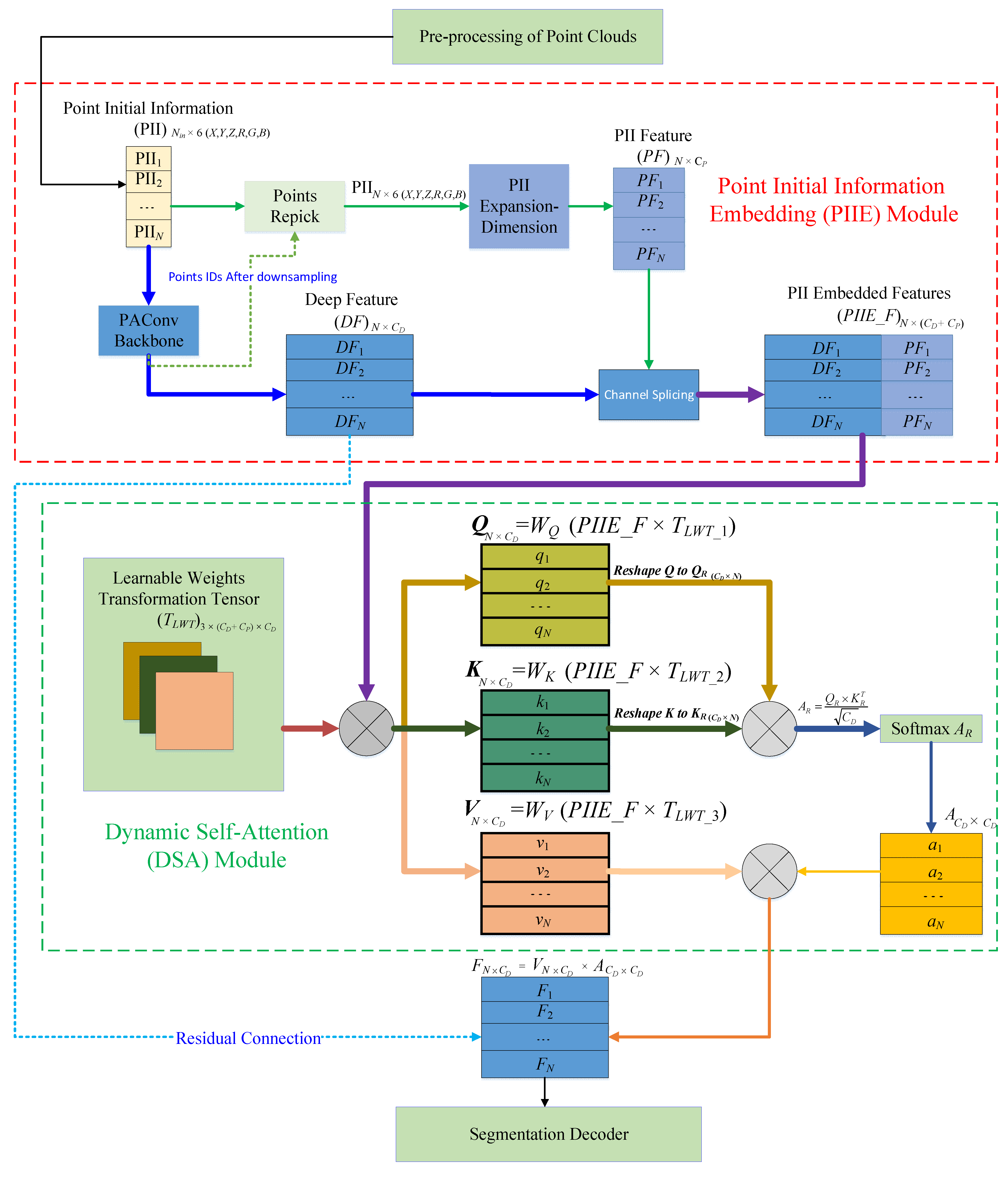
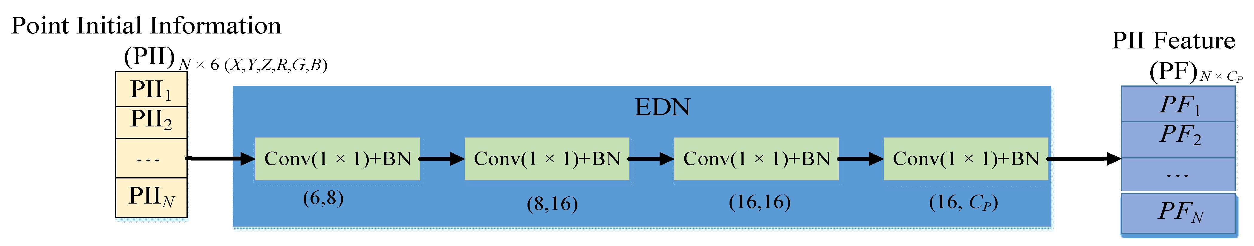
2.2. Point Initial Information Embedding
2.3. Dynamic Self-Attention
2.4. Loss Function Used in PIIE-DSA-Net
3. Experiments
3.1. Description of the Datasets
Statement of the Datasets
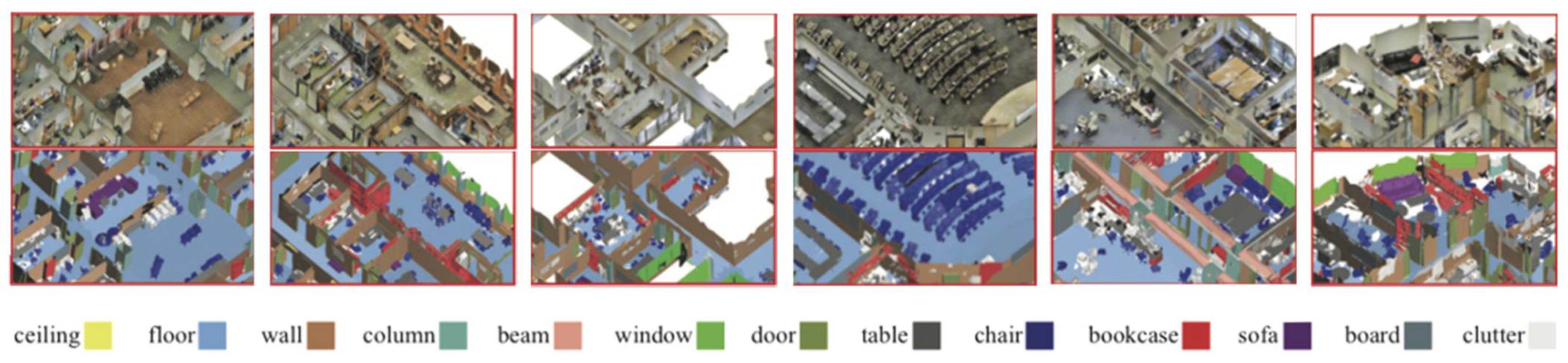
- Stanford Large-Scale 3D Indoor Spaces Dataset (S3DIS)
- 2.
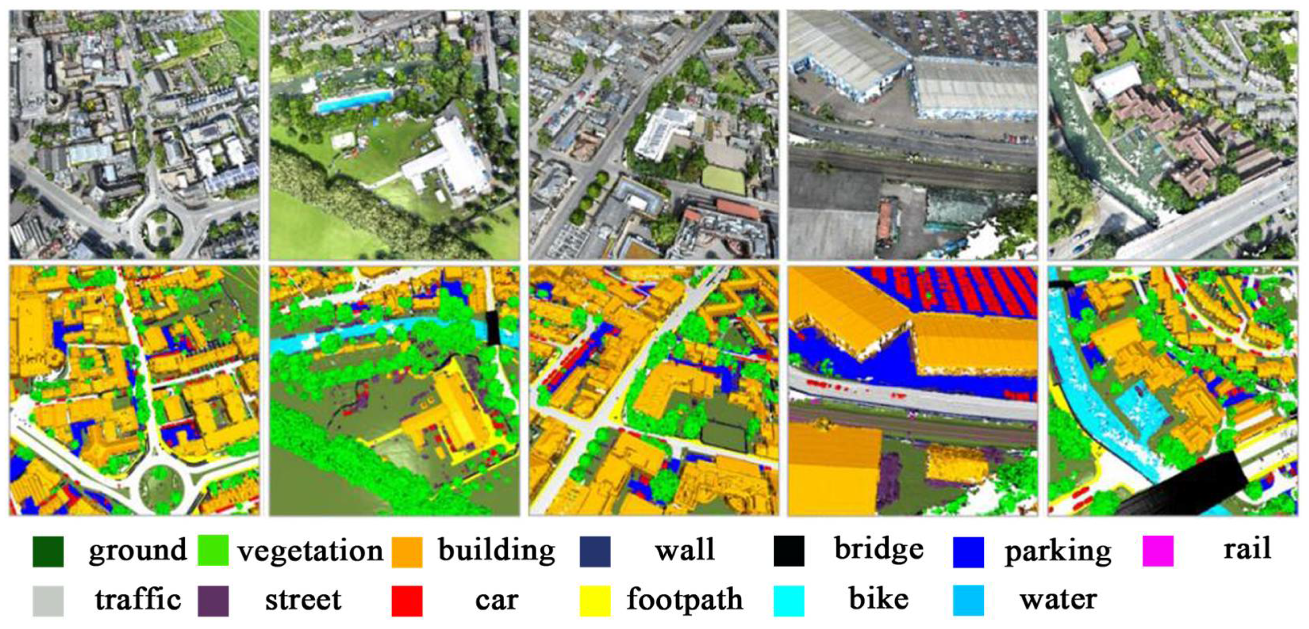
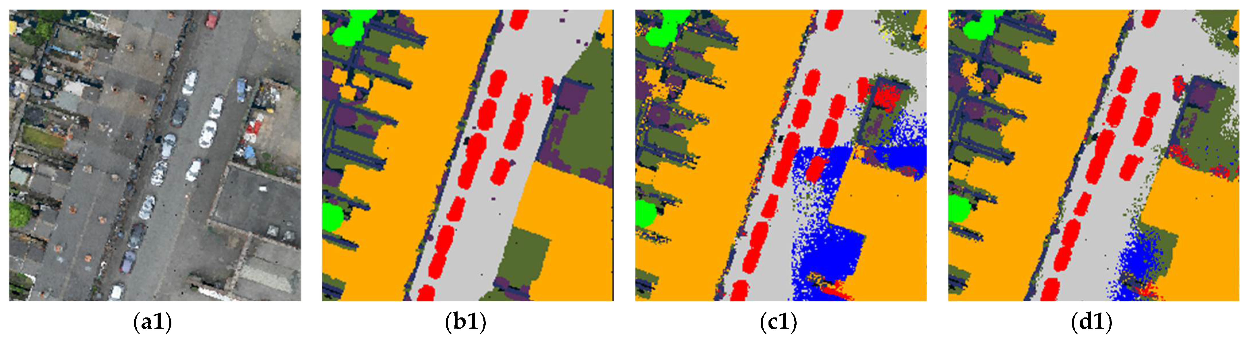
- SensatUrban dataset
- 3.
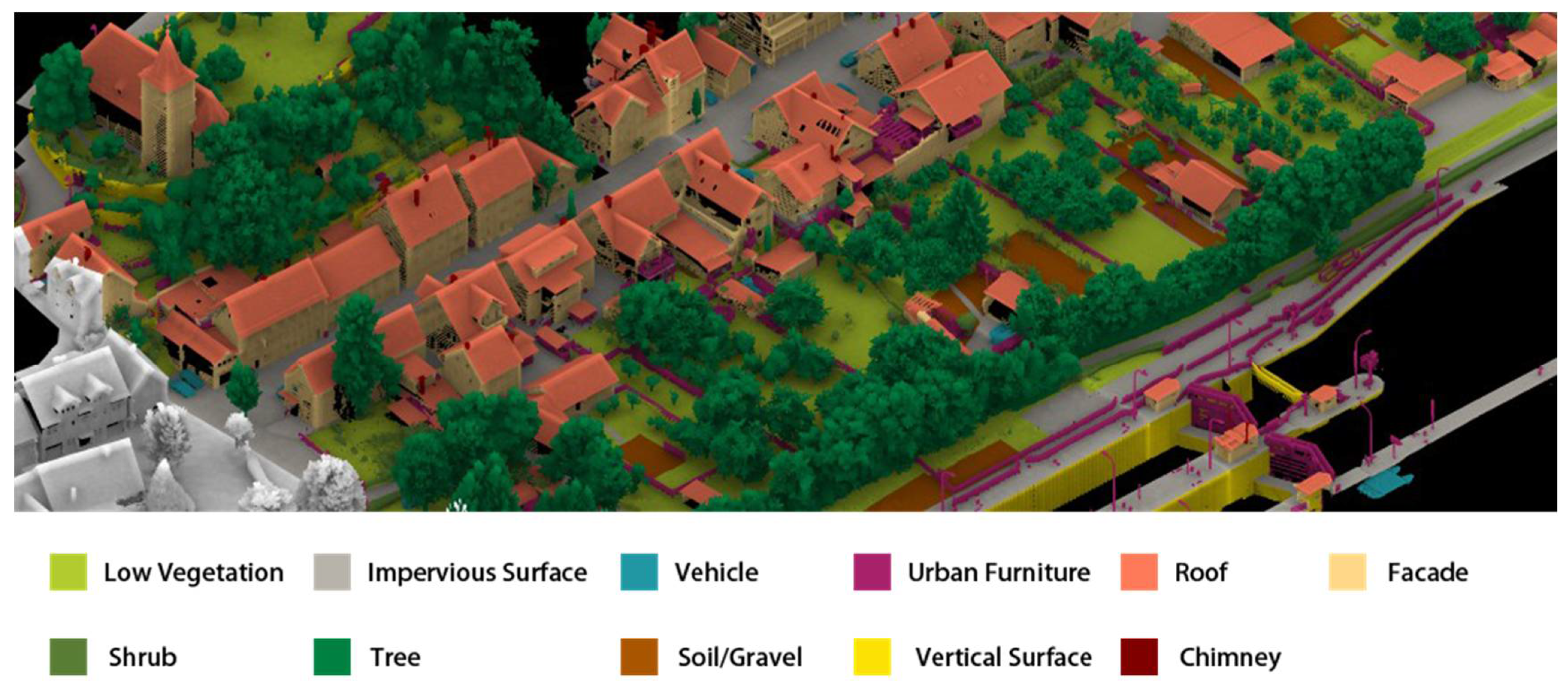
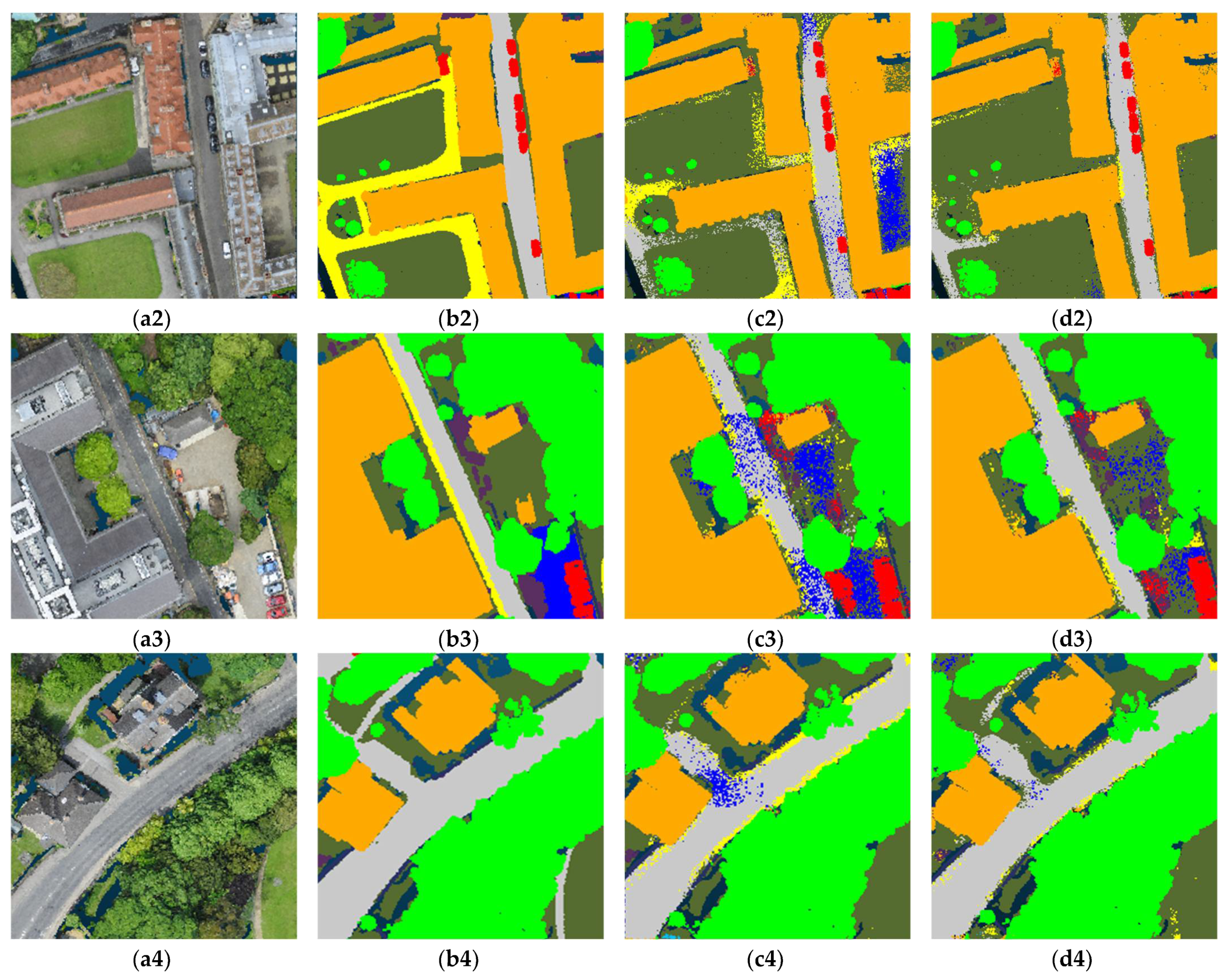
- Hessigheim 3D dataset
3.2. Evaluation Metrics
3.3. 3D Semantic Segmentation Experiments
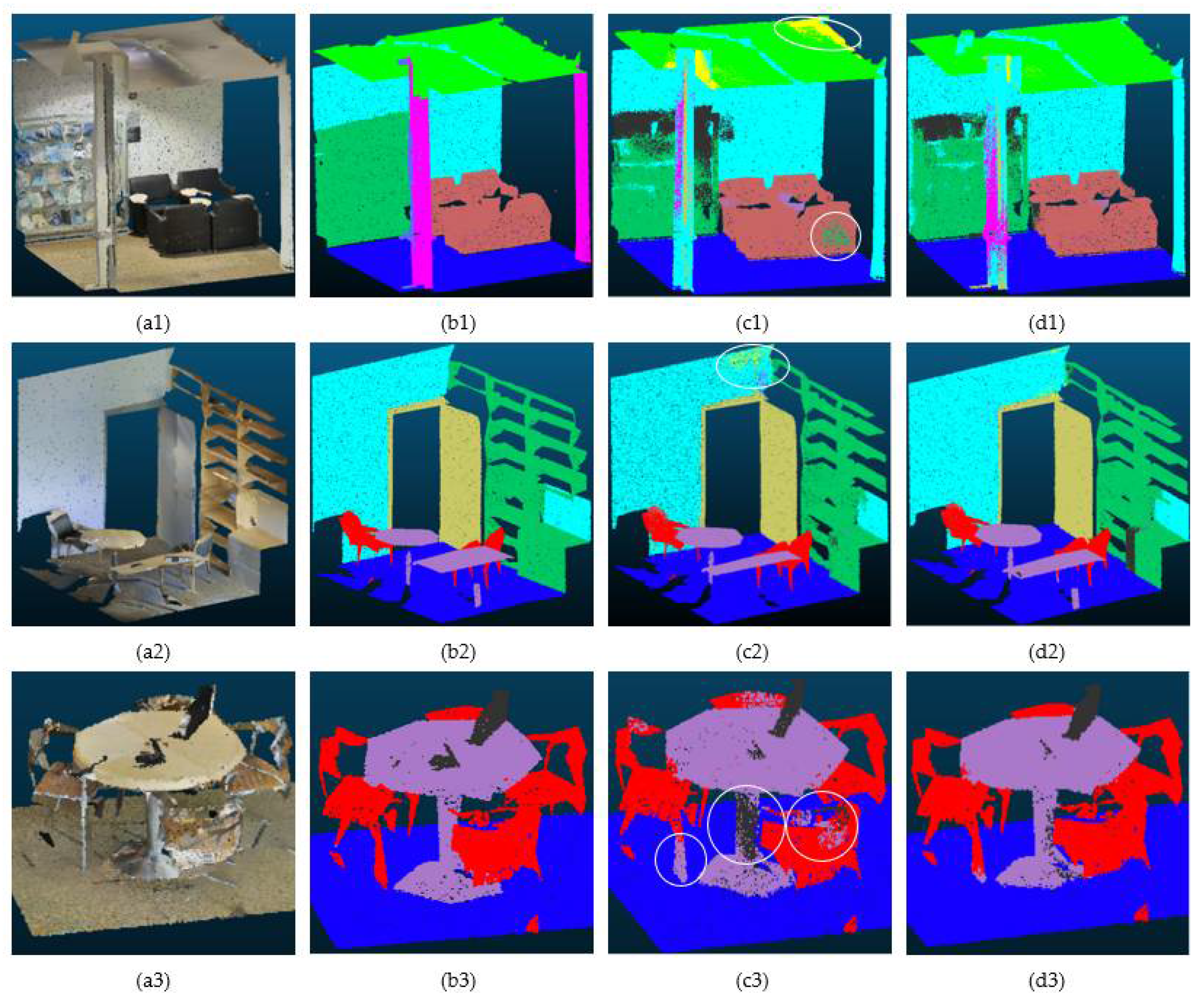
3.3.1. Performance of PIIE-DSA-Net on Indoor Dataset S3DIS
- Ablation experiments on the indoor dataset
3.3.2. Performance of PIIE-DSA-Net on the Outdoor Dataset SensatUrban and H3D
- Result analysis of SensatUrban dataset
- 2.
- Ablation experiments on the outdoor dataset
- 3.
- Result analysis for the H3D dataset
4. Conclusions and Discussion
Author Contributions
Funding
Data Availability Statement
Conflicts of Interest
References
- Hu, Q.; Wang, S.; Fu, C.; Ai, M.; Yu, D.; Wang, W. Fine Surveying and 3D Modeling Approach for Wooden Ancient Architecture via Multiple Laser Scanner Integration. Remote Sens. 2016, 8, 270. [Google Scholar] [CrossRef] [Green Version]
- Siranec, M.; Höger, M.; Otcenásová, A. Advanced Power Line Diagnostics Using Point Cloud Data-Possible Applications and Limits. Remote Sens. 2021, 13, 1880. [Google Scholar] [CrossRef]
- Çakir, A.; Akpancar, S. 3D Simultaneous Positioning and Mapping in Dark, Closed Spaces with an Autonomous Flying Robot. Acta Polytech. Hung. 2020, 17, 7–23. [Google Scholar] [CrossRef]
- Li, Y.; Ma, L.; Zhong, Z.; Liu, F.; Cao, D.; Li, J.; Chapman, M.A. Deep Learning for LiDAR Point Clouds in Autonomous Driving: A Review. IEEE Trans. Neural Netw. Learn. Syst. 2021, 32, 3412–3432. [Google Scholar] [CrossRef] [PubMed]
- Chen, Y.; Liu, G.; Xu, Y.; Pan, P.; Xing, Y. PointNet++ Network Architecture with Individual Point Level and Global Features on Centroid for ALS Point Cloud Classification. Remote Sens. 2021, 13, 472. [Google Scholar] [CrossRef]
- Elsner, P.; Dornbusch, U.; Thomas, I.; Amos, D.F.; Bovington, J.T.; Horn, D. Coincident beach surveys using UAS, vehicle mounted and airborne laser scanner: Point cloud inter-comparison and effects of surface type heterogeneity on elevation accuracies. Remote Sens. Environ. 2018, 208, 15–26. [Google Scholar] [CrossRef]
- Mathias, L. Mobile Laser Scanning Point Clouds. Gim International. Available online: https://www.gim-international.com/content/article/mobile-laser-scanning-point-clouds (accessed on 3 August 2017).
- Zhu, J.; Xu, Y.; Ye, Z.; Hoegner, L.; Stilla, U. Fusion of urban 3D point clouds with thermal attributes using MLS data and TIR image sequences. Infrared Phys. Technol. 2021, 113, 103622. [Google Scholar] [CrossRef]
- Babahajiani, P.; Fan, L.; Kämäräinen, J.; Gabbouj, M. Comprehensive Automated 3D Urban Environment Modelling Using Terrestrial Laser Scanning Point Cloud. In Proceedings of the 2016 IEEE Conference on Computer Vision and Pattern Recognition Workshops (CVPRW), Las Vegas, NV, USA, 26 June–1 July 2016; pp. 652–660. [Google Scholar]
- Poli, D.; Caravaggi, I. 3D modeling of large urban areas with stereo VHR satellite imagery: Lessons learned. Nat. Hazards 2013, 68, 53–78. [Google Scholar] [CrossRef]
- Xie, Y.; Tian, J.; Zhu, X.X. Linking Points With Labels in 3D: A Review of Point Cloud Semantic Segmentation. IEEE Geosci. Remote Sens. Magzine 2020, 8, 38–59. [Google Scholar] [CrossRef] [Green Version]
- Bello, S.A.; Yu, S.; Wang, C.; Adam, J.M.; Li, J. Review: Deep learning on 3D point clouds. Remote Sens. 2020, 12, 1729. [Google Scholar] [CrossRef]
- Han, X.; Jin, J.S.; Wang, M.; Jiang, W.; Gao, L.; Xiao, L. A review of algorithms for filtering the 3D point cloud. Signal Process. Image Commun. 2017, 57, 103–112. [Google Scholar]
- Cheng, S.; Chen, X.; He, X.; Liu, Z.; Bai, X. PRA-Net: Point Relation-Aware Network for 3D Point Cloud Analysis. IEEE Trans. Image Process. 2021, 30, 4436–4448. [Google Scholar] [CrossRef]
- Chen, Y.; Liu, X.; Xiao, Y.; Zhao, Q.; Wan, S. Three-Dimensional Urban Land Cover Classification by Prior-Level Fusion of LiDAR Point Cloud and Optical Imagery. Remote Sens. 2021, 13, 4928. [Google Scholar] [CrossRef]
- Wang, Y.; Shi, T.; Yun, P.; Tai, L.; Liu, M. PointSeg: Real-Time Semantic Segmentation Based on 3D LiDAR Point Cloud. arXiv 2018, arXiv:1807.06288. [Google Scholar]
- Milioto, A.; Vizzo, I.; Behley, J.; Stachniss, C. RangeNet ++: Fast and Accurate LiDAR Semantic Segmentation. In Proceedings of the 2019 IEEE/RSJ International Conference on Intelligent Robots and Systems (IROS), Macau, China, 3–8 November 2019; pp. 4213–4220. [Google Scholar]
- Lyu, Y.; Huang, X.; Zhang, Z. Learning to Segment 3D Point Clouds in 2D Image Space. In Proceedings of the 2020 IEEE/CVF Conference on Computer Vision and Pattern Recognition (CVPR), Seattle, WA, USA, 13–19 June 2020; pp. 12252–12261. [Google Scholar]
- Poux, F.; Billen, R. Voxel-based 3D Point Cloud Semantic Segmentation: Unsupervised Geometric and Relationship Featuring vs Deep Learning Methods. ISPRS Int. J. Geo Inf. 2019, 8, 213. [Google Scholar] [CrossRef] [Green Version]
- Liu, Z.; Tang, H.; Lin, Y.; Han, S. Point-Voxel CNN for Efficient 3D Deep Learning. arXiv 2019, arXiv:1907.03739. [Google Scholar]
- Graham, B.; Engelcke, M.; Maaten, L.V. 3D Semantic Segmentation with Submanifold Sparse Convolutional Networks. In Proceedings of the 2018 IEEE/CVF Conference on Computer Vision and Pattern Recognition, Salt Lake City, UT, USA, 18–22 June 2018; pp. 9224–9232. [Google Scholar]
- Le, T.; Duan, Y. PointGrid: A Deep Network for 3D Shape Understanding. In Proceedings of the 2018 IEEE/CVF Conference on Computer Vision and Pattern Recognition, Salt Lake City, UT, USA, 18–22 June 2018; pp. 9204–9214. [Google Scholar]
- Meng, H.; Gao, L.; Lai, Y.; Manocha, D. VV-Net: Voxel VAE Net With Group Convolutions for Point Cloud Segmentation. In Proceedings of the 2019 IEEE/CVF International Conference on Computer Vision (ICCV), Seoul, Korea, 10–17 October 2019; pp. 8499–8507. [Google Scholar]
- Triess, L.T.; Peter, D.; Rist, C.B.; Zöllner, J.M. Scan-based Semantic Segmentation of LiDAR Point Clouds: An Experimental Study. In Proceedings of the 2020 IEEE Intelligent Vehicles Symposium (IV), Las Vegas, NV, USA, 19 October–13 November 2020; pp. 1116–1121. [Google Scholar]
- Qi, C.; Su, H.; Mo, K.; Guibas, L.J. PointNet: Deep Learning on Point Sets for 3D Classification and Segmentation. In Proceedings of the 2017 IEEE Conference on Computer Vision and Pattern Recognition (CVPR), Honolulu, HI, USA, 21–26 July 2017; pp. 77–85. [Google Scholar]
- Qi, C.; Yi, L.; Su, H.; Guibas, L.J. PointNet++: Deep Hierarchical Feature Learning on Point Sets in a Metric Space. In Advances in Neural Information Processing Systems 30 (NIPS 2017); Neural Information Processing Systems Foundation, Inc.: La Jolla, CA, USA, 2017; Volume 30. [Google Scholar]
- Huang, Q.; Wang, W.; Neumann, U. Recurrent Slice Networks for 3D Segmentation of Point Clouds. In Proceedings of the 2018 IEEE/CVF Conference on Computer Vision and Pattern Recognition, Salt Lake City, UT, USA, 18–22 June 2018; pp. 2626–2635. [Google Scholar]
- Zhao, H.; Jiang, L.; Fu, C.; Jia, J. PointWeb: Enhancing Local Neighborhood Features for Point Cloud Processing. In Proceedings of the 2019 IEEE/CVF Conference on Computer Vision and Pattern Recognition (CVPR), Long Beach, CA, USA, 15–20 June 2019; pp. 5560–5568. [Google Scholar]
- Zhang, Z.; Hua, B.; Yeung, S. ShellNet: Efficient Point Cloud Convolutional Neural Networks Using Concentric Shells Statistics. In Proceedings of the 2019 IEEE/CVF International Conference on Computer Vision (ICCV), Seoul, Korea, 10–17 October 2019; pp. 1607–1616. [Google Scholar]
- Qian, G.; Hammoud, H.A.; Li, G.; Thabet, A.K.; Ghanem, B. ASSANet: An Anisotropic Separable Set Abstraction for Efficient Point Cloud Representation Learning. In Advances in Neural Information Processing Systems 34 (NeurIPS 2021); Neural Information Processing Systems Foundation, Inc.: La Jolla, CA, USA, 2021; Volume 34, pp. 28119–28130. [Google Scholar]
- Ran, H.; Liu, J.; Wang, C. Surface Representation for Point Clouds. arXiv 2022, arXiv:2205.05740. [Google Scholar]
- Qian, G.; Li, Y.; Peng, H.; Mai, J.; Hammoud, H.A.; Elhoseiny, M.; Ghanem, B. PointNeXt: Revisiting PointNet++ with Improved Training and Scaling Strategies. arXiv 2022, arXiv:2206.04670. [Google Scholar]
- Yan, X.; Zheng, C.; Li, Z.; Wang, S.; Cui, S. PointASNL: Robust Point Clouds Processing Using Nonlocal Neural Networks With Adaptive Sampling. In Proceedings of the 2020 IEEE/CVF Conference on Computer Vision and Pattern Recognition (CVPR), Seattle, WA, USA, 13–19 June 2020; pp. 5588–5597. [Google Scholar]
- Li, Y.; Bu, R.; Sun, M.; Wu, W.; Di, X.; Chen, B. PointCNN: Convolution On X-Transformed Points. In Advances in Neural Information Processing Systems 31 (NeurIPS 2018); Neural Information Processing Systems Foundation, Inc.: La Jolla, CA, USA, 2018; Volume 31. [Google Scholar]
- Thomas, H.; Qi, C.; Deschaud, J.; Marcotegui, B.; Goulette, F.; Guibas, L.J. KPConv: Flexible and Deformable Convolution for Point Clouds. In Proceedings of the 2019 IEEE/CVF International Conference on Computer Vision (ICCV), Seoul, Korea, 10–17 October 2019; pp. 6410–6419. [Google Scholar]
- Hu, Q.; Yang, B.; Xie, L.; Rosa, S.; Guo, Y.; Wang, Z.; Trigoni, A.; Markham, A. RandLA-Net: Efficient Semantic Segmentation of Large-Scale Point Clouds. In Proceedings of the 2020 IEEE/CVF Conference on Computer Vision and Pattern Recognition (CVPR), Seattle, WA, USA, 13–19 June 2020; pp. 11105–11114. [Google Scholar]
- Boulch, A. ConvPoint: Continuous convolutions for point cloud processing. Comput. Graph. 2020, 88, 24–34. [Google Scholar] [CrossRef] [Green Version]
- Xu, M.; Ding, R.; Zhao, H.; Qi, X. PAConv: Position Adaptive Convolution with Dynamic Kernel Assembling on Point Clouds. In Proceedings of the 2021 IEEE/CVF Conference on Computer Vision and Pattern Recognition (CVPR), Nashville, TN, USA, 20–25 June 2021; pp. 3172–3181. [Google Scholar]
- Deng, S.; Dong, Q. GA-NET: Global Attention Network for Point Cloud Semantic Segmentation. IEEE Signal Process. Lett. 2021, 28, 1300–1304. [Google Scholar] [CrossRef]
- Chen, X.; Li, Y.; Fan, J.; Wang, R. RGAM: A novel network architecture for 3D point cloud semantic segmentation in indoor scenes. Inf. Sci. 2021, 571, 87–103. [Google Scholar] [CrossRef]
- Geng, X.; Ji, S.; Lu, M.; Zhao, L. Multi-Scale Attentive Aggregation for LiDAR Point Cloud Segmentation. Remote Sens. 2021, 13, 691. [Google Scholar] [CrossRef]
- Marsocci, V.; Scardapane, S.; Komodakis, N. MARE: Self-Supervised Multi-Attention REsu-Net for Semantic Segmentation in Remote Sensing. Remote Sens. 2021, 13, 3275. [Google Scholar] [CrossRef]
- Chen, Z.; Li, D.; Fan, W.; Guan, H.; Wang, C.; Li, J. Self-Attention in Reconstruction Bias U-Net for Semantic Segmentation of Building Rooftops in Optical Remote Sensing Images. Remote Sens. 2021, 13, 2524. [Google Scholar] [CrossRef]
- Li, J.; Chen, B.M.; Lee, G.H. SO-Net: Self-Organizing Network for Point Cloud Analysis. In Proceedings of the 2018 IEEE/CVF Conference on Computer Vision and Pattern Recognition, Salt Lake City, UT, USA, 18–22 June 2018; pp. 9397–9406. [Google Scholar]
- Zhao, H.; Jiang, L.; Jia, J.; Torr, P.H.; Koltun, V. Point Transformer. In Proceedings of the 2021 IEEE/CVF International Conference on Computer Vision (ICCV), Montreal, BC, Canada, 11–17 October 2021; pp. 16239–16248. [Google Scholar]
- Cheng, Z.; Wan, H.; Shen, X.; Wu, Z. PatchFormer: An Efficient Point Transformer with Patch Attention. In Proceedings of the 2021 IEEE/CVF Conference on Computer Vision and Pattern Recognition, Nashville, TN, USA, 20–25 June 2021. [Google Scholar]
- Lai, X.; Liu, J.; Jiang, L.; Wang, L.; Zhao, H.; Liu, S.; Qi, X.; Jia, J. Stratified Transformer for 3D Point Cloud Segmentation. arXiv 2022, arXiv:2203.14508. [Google Scholar]
- Wang, Y.; Sun, Y.; Liu, Z.; Sarma, S.E.; Bronstein, M.M.; Solomon, J.M. Dynamic Graph CNN for Learning on Point Clouds. ACM Trans. Graph. (TOG) 2019, 38, 1–12. [Google Scholar] [CrossRef] [Green Version]
- Wang, C.; Samari, B.; Siddiqi, K. Local Spectral Graph Convolution for Point Set Feature Learning. In Proceedings of the European Conference on Computer Vision (ECCV), Munich, Germany, 8–14 September 2018. [Google Scholar]
- Landrieu, L.; Boussaha, M. Point Cloud Oversegmentation With Graph-Structured Deep Metric Learning. In Proceedings of the 2019 IEEE/CVF Conference on Computer Vision and Pattern Recognition (CVPR), Long Beach, CA, USA, 15–20 June 2019; pp. 7432–7441. [Google Scholar]
- Xie, L.; Furuhata, T.; Shimada, K. Multi-Resolution Graph Neural Network for Large-Scale Pointcloud Segmentation. arXiv 2020, arXiv:2009.08924. [Google Scholar]
- Lu, T.; Wang, L.; Wu, G. CGA-Net: Category Guided Aggregation for Point Cloud Semantic Segmentation. In Proceedings of the 2021 IEEE/CVF Conference on Computer Vision and Pattern Recognition (CVPR), Nashville, TN, USA, 20–25 June 2021; pp. 11688–11697. [Google Scholar]
- Qiu, S.; Anwar, S.; Barnes, N. Semantic Segmentation for Real Point Cloud Scenes via Bilateral Augmentation and Adaptive Fusion. In Proceedings of the 2021 IEEE/CVF Conference on Computer Vision and Pattern Recognition (CVPR), Nashville, TN, USA, 20–25 June 2021; pp. 1757–1767. [Google Scholar]
- Robert, D.L.; Vallet, B.; Landrieu, L. Learning Multi-View Aggregation In the Wild for Large-Scale 3D Semantic Segmentation. arXiv 2022, arXiv:2204.07548. [Google Scholar]
- Tang, L.; Zhan, Y.; Chen, Z.; Yu, B.; Tao, D. Contrastive Boundary Learning for Point Cloud Segmentation. arXiv 2022, arXiv:2203.05272. [Google Scholar]
- Zhao, L.; Tao, W. JSNet: Joint Instance and Semantic Segmentation of 3D Point Clouds. In Proceedings of the AAAI Conference on Artificial Intelligence, New York, NY, USA, 7–12 February 2020. [Google Scholar]
- Jiang, L.; Zhao, H.; Liu, S.; Shen, X.; Fu, C.; Jia, J. Hierarchical Point-Edge Interaction Network for Point Cloud Semantic Segmentation. In Proceedings of the 2019 IEEE/CVF International Conference on Computer Vision (ICCV), Seoul, Korea, 10–17 October 2019; pp. 10432–10440. [Google Scholar]
- Shaw, P.; Uszkoreit, J.; Vaswani, A. Self-Attention with Relative Position Representations. arXiv 2018, arXiv:1803.02155. [Google Scholar]
- He, K.; Zhang, X.; Ren, S.; Sun, J. Delving Deep into Rectifiers: Surpassing Human-Level Performance on ImageNet Classification. In Proceedings of the 2015 IEEE International Conference on Computer Vision (ICCV), Santiago, Chile, 7–13 December 2015; pp. 1026–1034. [Google Scholar]
- Voita, E.; Talbot, D.; Moiseev, F.; Sennrich, R.; Titov, I. Analyzing Multi-Head Self-Attention: Specialized Heads Do the Heavy Lifting, the Rest Can Be Pruned. arXiv 2019, arXiv:1905.09418. [Google Scholar]
- Armeni, I.; Sener, O.; Zamir, A.R.; Jiang, H.; Brilakis, I.K.; Fischer, M.; Savarese, S. 3D Semantic Parsing of Large-Scale Indoor Spaces. In Proceedings of the 2016 IEEE Conference on Computer Vision and Pattern Recognition (CVPR), Las Vegas, NV, USA, 27–30 June 2016; pp. 1534–1543. [Google Scholar]
- Hu, Q.; Yang, B.; Khalid, S.; Xiao, W.; Trigoni, A.; Markham, A. Towards Semantic Segmentation of Urban-Scale 3D Point Clouds: A Dataset, Benchmarks and Challenges. In Proceedings of the 2021 IEEE/CVF Conference on Computer Vision and Pattern Recognition (CVPR), Nashville, TN, USA, 20–25 June 2021; pp. 4975–4985. [Google Scholar]
- Kölle, M.; Laupheimer, D.; Schmohl, S.; Haala, N.; Rottensteiner, F.; Wegner, J.D.; Ledoux, H. The Hessigheim 3D (H3D) Benchmark on Semantic Segmentation of High-Resolution 3D Point Clouds and Textured Meshes from UAV LiDAR and Multi-View-Stereo. arXiv 2021, arXiv:2102.05346. [Google Scholar] [CrossRef]


| Categories/Test Area | Area1 | Area2 | Area3 | Area4 | Area5 | Area6 |
|---|---|---|---|---|---|---|
| ceiling | 97.98 | 90.67 | 95.94 | 93.26 | 93.27 | 96.31 |
| floor | 97.24 | 77.66 | 98.30 | 97.38 | 98.51 | 97.33 |
| wall | 93.61 | 79.62 | 83.00 | 78.11 | 82.75 | 85.31 |
| column | 86.87 | 31.80 | 23.26 | 34.58 | 28.42 | 62.85 |
| beam | 93.05 | 15.25 | 62.10 | 0.87 | 0.00 | 81.75 |
| window | 94.30 | 54.55 | 82.96 | 33.23 | 62.26 | 85.63 |
| door | 94.51 | 65.72 | 91.93 | 64.12 | 67.63 | 89.64 |
| table | 86.91 | 60.48 | 77.70 | 63.04 | 79.01 | 78.01 |
| chair | 93.30 | 28.54 | 83.90 | 72.64 | 88.86 | 80.95 |
| bookcase | 94.59 | 28.00 | 75.13 | 63.02 | 60.65 | 53.52 |
| sofa | 90.26 | 47.55 | 75.53 | 54.61 | 74.51 | 75.46 |
| board | 93.18 | 19.75 | 90.21 | 45.20 | 74.98 | 81.26 |
| clutter | 88.27 | 37.13 | 75.53 | 58.72 | 58.86 | 71.66 |
| mIoU | 92.62 | 48.98 | 78.11 | 58.37 | 66.90 | 79.98 |
| mAcc | 96.23 | 62.41 | 86.46 | 68.15 | 73.90 | 88.35 |
| OA | 96.77 | 79.46 | 91.59 | 85.86 | 89.44 | 92.24 |
| Rank | Methods | mIoU | mAcc | OA |
|---|---|---|---|---|
| 1 | RepSurf-U [31] | 74.3 | 82.6 | 90.8 |
| 2 | PointNeXt [32] | 74.9 | 83.0 | 90.3 |
| 3 | PointTransformer [45] | 73.5 | 81.9 | 90.2 |
| 4 | DeepViewAgg [54] | 74.7 | 83.8 | 90.1 |
| 5 | CBL [55] | 73.1 | 79.4 | 89.6 |
| 6 | BAAF-Net [53] | 72.2 | 83.1 | 88.9 |
| 7 | PIIE-DSA-net (OURS) | 71.66 | 81.24 | 88.89 |
| 8 | PointASNL [33] | 68.7 | 79.0 | 88.8 |
| 9 | ConvPoint [37] | 68.2 | N/A | 88.8 |
| 10 | JSNet [56] | 61.7 | 71.7 | 88.7 |
| Categories/Methods | PointNet | PointNet++ | PointCNN | KPconv Rigid | RandLA-Net | PAConv | PIIE-DSA-Net |
|---|---|---|---|---|---|---|---|
| ceiling | 88.80 | 91.31 | 92.31 | 92.6 | 91.69 | 94.55 | 93.72 |
| floor | 97.33 | 96.92 | 98.24 | 97.3 | 96.90 | 98.59 | 98.51 |
| wall | 69.80 | 78.73 | 79.41 | 81.4 | 78.45 | 82.37 | 82.75 |
| column | 3.92 | 15.99 | 17.60 | 16.5 | 27.07 | 26.43 | 28.42 |
| beam | 0.05 | 0.00 | 0.00 | 0.00 | 0.00 | 0.00 | 0.00 |
| window | 46.26 | 54.93 | 22.77 | 54.5 | 64.19 | 57.96 | 62.26 |
| door | 10.76 | 31.88 | 62.09 | 69.5 | 37.53 | 59.96 | 67.63 |
| table | 52.61 | 83.52 | 80.59 | 90.1 | 73.97 | 89.73 | 79.01 |
| chair | 58.93 | 74.62 | 74.39 | 80.2 | 83.94 | 80.44 | 88.86 |
| bookcase | 40.28 | 67.24 | 66.67 | 74.6 | 66.39 | 74.32 | 60.65 |
| sofa | 5.85 | 49.31 | 31.67 | 66.4 | 67.94 | 69.80 | 74.51 |
| board | 26.38 | 54.15 | 62.05 | 63.7 | 61.96 | 73.50 | 74.98 |
| clutter | 33.22 | 45.89 | 56.74 | 58.1 | 50.37 | 57.72 | 58.86 |
| mIoU | 41.09 | 57.27 | 57.26 | 65.4 | 61.57 | 66.58 | 66.90 |
| mAcc | 49.98 | 63.54 | 63.86 | 70.9 | 71.50 | 73.00 | 73.90 |
| Rank | Methods | mIoU | mAcc | OA |
|---|---|---|---|---|
| 1 | StratifiedFormer [61] | 72.0 | 78.1 | 91.5 |
| 2 | PointNeXt [32] | 71.1 | 77.2 | 91.0 |
| 3 | PointTransformer [45] | 70.4 | 76.5 | 90.8 |
| 4 | CBL [55] | 69.4 | 75.2 | 90.6 |
| 5 | RepSurf-U [31] | 68.9 | 76.0 | 90.2 |
| 6 | PIIE-DSA-net (OURS) | 66.9 | 73.9 | 89.44 |
| 7 | BAAF-Net [53] | 65.4 | 73.1 | 88.9 |
| 8 | MuG-net [51] | 63.5 | N/A | 88.1 |
| 9 | SSP + SPG [50] | 61.7 | 68.2 | 87.9 |
| 10 | HPEIN [57] | 61.85 | 68.3 | 87.18 |
| S3DIS | Module Ablation | PIIE Transformation Methods | Selection of Multi-Head Attention Operation | PIIE-DSA-Net | |||
|---|---|---|---|---|---|---|---|
| PAConv | PAConv + PIIE | Convolution Transform | Full-Connection Transform | Two-Head Attention | Four-Head Attention | ||
| ceiling | 94.55 | 93.67 | 93.63 | 94.01 | 92.58 | 94.90 | 93.72 |
| floor | 98.59 | 98.50 | 98.21 | 98.05 | 98.51 | 98.44 | 98.51 |
| wall | 82.37 | 82.63 | 82.27 | 82.36 | 82.30 | 82.14 | 82.75 |
| column | 26.43 | 32.62 | 20.04 | 21.49 | 26.41 | 17.34 | 28.42 |
| beam | 0.00 | 0.00 | 0.00 | 0.00 | 0.00 | 0.00 | 0.00 |
| window | 57.96 | 59.55 | 59.50 | 60.93 | 59.50 | 57.52 | 62.26 |
| door | 59.96 | 65.92 | 67.95 | 68.72 | 62.80 | 54.77 | 67.63 |
| table | 80.44 | 79.64 | 79.13 | 77.29 | 79.31 | 80.10 | 79.01 |
| chair | 89.73 | 88.34 | 86.13 | 85.68 | 88.21 | 88.54 | 88.86 |
| bookcase | 74.32 | 60.92 | 64.12 | 59.67 | 58.23 | 61.02 | 60.65 |
| sofa | 69.80 | 74.40 | 72.28 | 71.20 | 73.89 | 75.49 | 74.51 |
| board | 73.50 | 71.67 | 72.36 | 69.55 | 75.71 | 73.67 | 74.98 |
| clutter | 57.72 | 59.12 | 58.36 | 58.48 | 56.96 | 58.82 | 58.86 |
| mIoU | 66.58 | 66.69 | 65.69 | 65.19 | 65.72 | 64.83 | 66.90 |
| mAcc | 73.00 | 73.98 | 71.96 | 71.65 | 72.13 | 70.87 | 73.90 |
| SensatUrban | Module Ablation | PIIE Transformation Methods | Selection of Multi-Head Attention Operation | PIIE-DSA-Net | |||
|---|---|---|---|---|---|---|---|
| PAConv | PAConv + PIIE | Convolution Transform | Full-Connection Transform | Two-Head Attention | Four-Head Attention | ||
| ground | 72.11 | 73.53 | 73.10 | 74.48 | 74.43 | 73.37 | 73.92 |
| vegetation | 97.54 | 97.30 | 97.11 | 97.72 | 97.86 | 97.56 | 97.69 |
| building | 93.01 | 92.90 | 91.98 | 93.65 | 92.92 | 93.22 | 93.05 |
| wall | 44.43 | 49.98 | 49.68 | 47.22 | 50.71 | 49.69 | 49.81 |
| bridge | 5.78 | 3.77 | 2.42 | 0.01 | 2.01 | 6.73 | 17.43 |
| parking | 39.94 | 40.21 | 37.51 | 43.27 | 43.11 | 41.52 | 40.60 |
| rail | 0.00 | 0.00 | 0.00 | 0.00 | 0.00 | 0.00 | 0.00 |
| car | 73.04 | 77.87 | 77.09 | 75.90 | 77.66 | 77.56 | 77.75 |
| footpath | 21.78 | 23.75 | 21.68 | 24.31 | 24.66 | 22.58 | 24.57 |
| bike | 0.00 | 0.00 | 0.00 | 0.00 | 0.00 | 0.00 | 0.00 |
| water | 57.97 | 63.87 | 60.22 | 58.62 | 62.87 | 62.47 | 57.10 |
| traffic road | 58.78 | 63.00 | 59.97 | 62.96 | 62.99 | 62.07 | 61.45 |
| Street furniture | 29.42 | 33.78 | 33.64 | 32.54 | 32.52 | 32.68 | 31.38 |
| mIoU | 45.68 | 47.69 | 46.49 | 46.98 | 47.82 | 47.65 | 48.09 |
| mAcc | 53.76 | 55.03 | 53.73 | 54.79 | 54.83 | 54.98 | 55.16 |
| Categories | PAConv | PIIE-DSA-Net |
|---|---|---|
| Low vegetation | 74 | 81 |
| Impervious Surface | 90 | 84 |
| Vehicle | 66 | 75 |
| Urban Furniture | 43 | 48 |
| Roof | 94 | 94 |
| Facade | 77 | 71 |
| Shrub | 55 | 63 |
| Tree | 96 | 95 |
| Soll/Gravel | 41 | 58 |
| Vertical Surface | 68 | 74 |
| Chimney | 100 | 85 |
| mIoU | 64.09 | 75.27 |
| OA | 74 | 81 |
Publisher’s Note: MDPI stays neutral with regard to jurisdictional claims in published maps and institutional affiliations. |
© 2022 by the authors. Licensee MDPI, Basel, Switzerland. This article is an open access article distributed under the terms and conditions of the Creative Commons Attribution (CC BY) license (https://creativecommons.org/licenses/by/4.0/).
Share and Cite
Gao, F.; Yan, Y.; Lin, H.; Shi, R. PIIE-DSA-Net for 3D Semantic Segmentation of Urban Indoor and Outdoor Datasets. Remote Sens. 2022, 14, 3583. https://doi.org/10.3390/rs14153583
Gao F, Yan Y, Lin H, Shi R. PIIE-DSA-Net for 3D Semantic Segmentation of Urban Indoor and Outdoor Datasets. Remote Sensing. 2022; 14(15):3583. https://doi.org/10.3390/rs14153583
Chicago/Turabian StyleGao, Fengjiao, Yiming Yan, Hemin Lin, and Ruiyao Shi. 2022. "PIIE-DSA-Net for 3D Semantic Segmentation of Urban Indoor and Outdoor Datasets" Remote Sensing 14, no. 15: 3583. https://doi.org/10.3390/rs14153583