Ocean Wave Inversion Based on a Ku/Ka Dual-Band Airborne Interferometric Imaging Radar Altimeter

Abstract

Ocean wave parameters (OWPs), including wave propagation direction (WPD), significant wave height (SWH), and main wave wavelength (MWW) can be typically retrieved using an interferometric imaging radar altimeter (InIRA). However, the inversion accuracy of ocean waves in Ku (15.8 GHz) and Ka (35.8 GHz) bands has not yet been evaluated due to the lack of field observation data. In this paper, to assess the inversion accuracy of OWPs in Ku and Ka bands, an airborne observation experiment using simultaneous Ku and Ka bands was carried out for the first time in Rizhao, Shandong Province, China. A dual-band InIRA (DInIRA) was configured with small incidence angles (4°–18°) and a Global Navigation Satellite System (GNSS) buoy; a mobile weather station was placed at the intersection of the plane routes for validation. Afterward, the WPD, SWH, and MWW were retrieved based on the imaging of sea surface height. As compared with the field in situ data, the WPD inversion results of main wind wave were found to be consistent with the measurement environmental wind direction. The SWH inversion biases, retrieved by the Ku and Ka bands, were 0.38 m and 0.27 m; the MWW inversion biases for the swells were equal to 16.75 m and 3.67 m; and the MWW inversion biases about the wind waves were 2.32 m and 0.57 m. Ultimately, it was established that the OWPs could be effectively retrieved by the DInIRA, and the inversion accuracy of the SWH and the MWW in the Ka band outperformed that in the Ku band.

1. Introduction

The study of ocean waves is a hot topic in oceanographic research. In this respect, currently, satellite altimetry has been introduced as an effective technique for detecting ocean waves. The traditional satellite-based radar altimetry technology, developed in the 1960s, is a practical approach for this purpose since it can measure sea surface height (SSH) [1]. However, traditional altimeters can simply estimate the significant wave height (SWH) of a target sea area, but fail to retrieve other ocean wave parameters, such as the wave propagation direction (WPD) and the main wave wavelength (MWW) [2,3].

As well, synthetic aperture radar (SAR) is widely used to detect ocean waves, due to its unique two-dimensional (2-D) imaging mechanism [4]. Two-dimensional ocean wave spectra (OWS) can be retrieved based on SAR images, and the WPD, SWH, MWW, as well as other related parameters can be further extracted using the OWS [5,6,7,8]. Inversion methods based on OWS according to SAR images have been correspondingly developed to a great extent, mostly depending on modulation functions. However, modulus and phase calculations in these functions are relatively rough [9], limiting the inversion accuracy of ocean waves.

The interferometric synthetic aperture radar (InSAR) is also an important tool for detecting ocean waves. Scheulz-Stellenfleth et al., (2001) [10] simulated a distorted digital elevation model (DEM) based on OWS and a cross-track InSAR (XTI-SAR) imaging model, and found that the SWH error was within 10% for the low-amplitude swells, and the error was related to the WPD. In the same year, Scheulz-Stellenfleth et al. [11] calculated SSH using airborne X-band XTI-SAR data, and demonstrated that SWH estimated in accordance with the DEM was similar to the results inversed by the buoy for the weak nonlinear imaging. However, the microwave scattering signals of the targets in the ocean were closely related to the wind field at moderate incidence angles, and the anisotropy and asymmetry [12] on the upwind/crosswind could reduce the inversion accuracy of the ocean waves.

In addition, Jackson et al., (1985) [13] proposed a theory to measure ocean waves at small incidence angles. Accordingly, observations at small incidence angles could moderate the requirements of the radar transmit power and the gain of the antenna, while ensuring target homogeneity, and the ocean targets in the signal overlay area were primarily of specular scattering. Rodriguez et al., (1999) [14] correspondingly proposed a new sensor, named the imaging radar altimeter (InIRA), which could achieve high inversion accuracy of ocean waves due to its small incidence angles. Roger Fjørtoft et al., (2014) [15] further conducted the first Ka-band InIRA experiment, which proved the typical characteristics of Ka-band InIRA images, and then assessed the superiority of satellite-based Ka band for detecting ocean waves. In 2016, successful operation of the Tiangong-II InIRA sensor was the first to assess the effectiveness for detecting ocean waves using the Ku band at small incidence angles [16]. In addition, the forthcoming launch of the Surface Water and Ocean Topography (SWOT) satellite was equipped with a Ka-band InIRA to obtain high inversion accuracy of ocean waves. AirSWOT is an airborne instrument for supporting the SWOT mission, and it plays a key role in SWOT mission development. In recent years, some experiments have been conducted on water surface elevation reconstruction and algorithm development based on the actual data of AirSWOT, which have indicated that the AirSWOT has high measurement accuracy [17,18,19,20]. However, there are many challenges [21,22] facing observations using Ka band. For instance, Ka-band electromagnetic waves are easily affected by the atmospheric environment, in addition, the posture stability of the satellite platform and the accuracy of the antenna orientation both have a significant impact on the observations based on the high-frequency bands.

A dual-band interferometric imaging radar altimeter (DInIRA) can address the abovementioned shortcomings. In 2018, the “Guanlan” ocean science satellite project was proposed by the Pilot National Laboratory for Marine Science and Technology of China to more effectively observe ocean waves and sub-mesoscale ocean phenomena. Of note, the “Guanlan” satellite would take the two-side observation geometry with multiple Ku-band beams less affected by the atmosphere and multiple Ka-band beams insensitive to the ionosphere, which could achieve a wider swath and a higher altimetric accuracy [22] as compared with single-frequency radars. In this sense, Tanelli et al., (2006) [23] compared the sea surface backscatter coefficients between the Ku and Ka bands for different incidence angles under special wind conditions, however, the results were not verified due to the lack of field observation data. Alamgir et al., (2021) [24] also compared the dependence on vector winds and sea surface temperature in Ku and Ka bands, and showed that the Ka band had a greater dependence on vector winds and sea surface temperature than the Ku at the low-to-medium wind speed area. Since no field observation data were available and even few studies have been conducted on the simultaneous observation of ocean waves using Ku and Ka bands worldwide, the bulk of the related literature was merely based on simulations [25,26]. The measurement mechanism of the InIRA has not been well established, and the performance of ocean wave inversion in Ku and Ka bands at small incidence angles is still unclear. As the airborne platform can verify the viability of InIRA technology in the ocean wave inversion, its application in theoretical assessments is crucial. This study conducted an airborne Ku/Ka dual-band simultaneous observation campaign on the sea area of Wanpingkou, Rizhao, Shandong Province, China, and aimed to analyze the performance of ocean wave inversion in Ku and Ka bands at small incidence angles based on airborne data. The remainder of this paper is organized as follows: in Section 2, we introduce the airborne DInIRA campaign and then process the echo data; in Section 3, we show the inversion results of the ocean waves and verify the results using the in situ data; in Section 4, we discuss the reliability of the inversion results, and analyze the characteristics of the satellite-based DInIRA; and finally, in Section 5, we provide a summary of the study.

2. Method

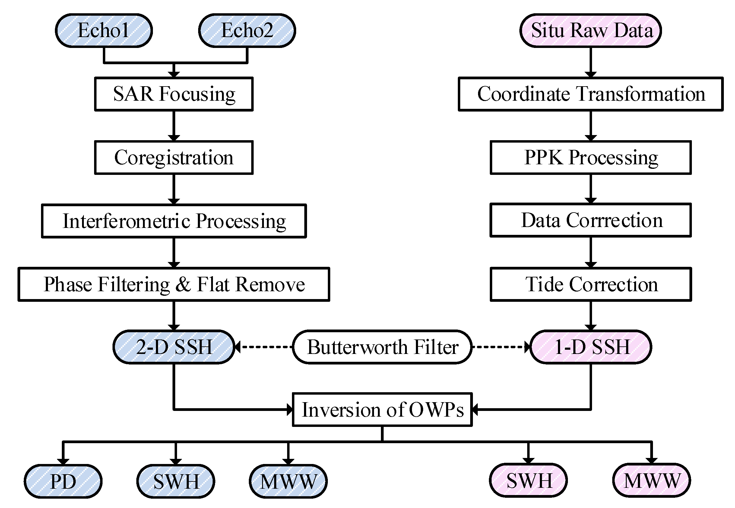
2.1. DInIRA Ocean Waves Inversion Methodology

The DInIRA exploited two sets of antennas (viz. four antennas) emitting different frequency bands for observation, and the pulse signals were emitted toward the ground-range direction at 6–18° (Ku) and 4–17° (Ka) incidence angles, respectively. As shown in Figure 1, the DInIRA measurement principle is similar to that in InSAR sensors.

Taking the Ku band (in black) as an example, where $A_1$ is the primary antenna and $A_2$ is the auxiliary antenna, $B$ denotes the baseline length, $\alpha$ refers to the baseline roll angle, and $r_1$ and $r_2$ are the distances from the primary and auxiliary antennas to point $P$, respectively. The angle of incidence relative to the target point $P$ on the sea surface is ${\theta }_1$, the $alt$ is the altitude of $A_1$ above the WGS-84 reference ellipsoid, and the height of the target point $P$ is $h$. The different phases are further measured by the $A_1$ and $A_2$ antennas due to the existence of the baseline. Therefore, the relationship between the slant range and the interference phase difference $\phi$ can be expressed as [27]:

$$\phi =\frac{2\pi \left(r_2-r_1\right)}{\lambda }=\frac{2\pi B\sin \left(\theta -\alpha \right)}{\lambda }$$

(1)

where $\lambda$ represents the return echo wavelength and the interference phase $\phi$ can be obtained by the interferometric processing. Finally, the elevation of the target point $P$ can be calculated according to Equation (2) by combining the information of the primary antenna parameters (including antenna height, baseline roll angle, and baseline length) [27]:

$$h=alt-r_1\cos \left(\frac{\pi }{2}+\alpha -\arccos \left(-\frac{\lambda \phi }{2\pi B}\right)\right)$$

(2)

Then, the SSH is inversed using the abovementioned methods, and the 2D OWS can be subsequently calculated based on the 2D Fourier transform ($FFT2$) [6]:

$$S\left(k_x,k_y\right)=\frac{{\left|FFT2\left(\mathsf{\Delta }h\right)\right|}^2}{mn\left(\frac{4{\pi }^2}{re{s}_{x}re{s}_y}\right)}$$

(3)

where $k_x$ and $k_y$ denote the wavenumber vectors in the ground-range (cross-track) direction and azimuth direction, respectively; $m$ and $n$ denote the number of pixels in two directions; and $re{s}_x$ and $re{s}_y$ refer to the pixel resolution in different directions. Finally, the ocean wave parameters (OWPs) are further extracted via the OWS [28]:

$$\mathrm{SWH}=4.005\times \sqrt{{{\displaystyle \iint }}^{ }S\left(k_x,k_y\right)d{k}_{x}d{k}_y}$$

(4)

$$\mathrm{MWW}=2\pi /k_p$$

(5)

where $k_p$ shows the wave number corresponding to the maximum spectral value in the OWS, and the WPD denotes the angle relative to the forward direction of the $k_x$ axis once $k=k_p$.

In addition, the main wave period (MWP) can be obtained based on the dispersion formula [29]:

$$\mathrm{MWP}=\frac{2\pi }{{\omega }_p}$$

(6)

where ${\omega }_p=\sqrt{g{k}_p\tanh \left(h{k}_p\right)}$, $g$ denotes the gravity constant, and $h$ is the depth of water.

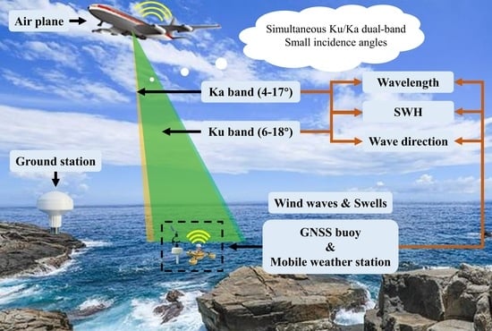
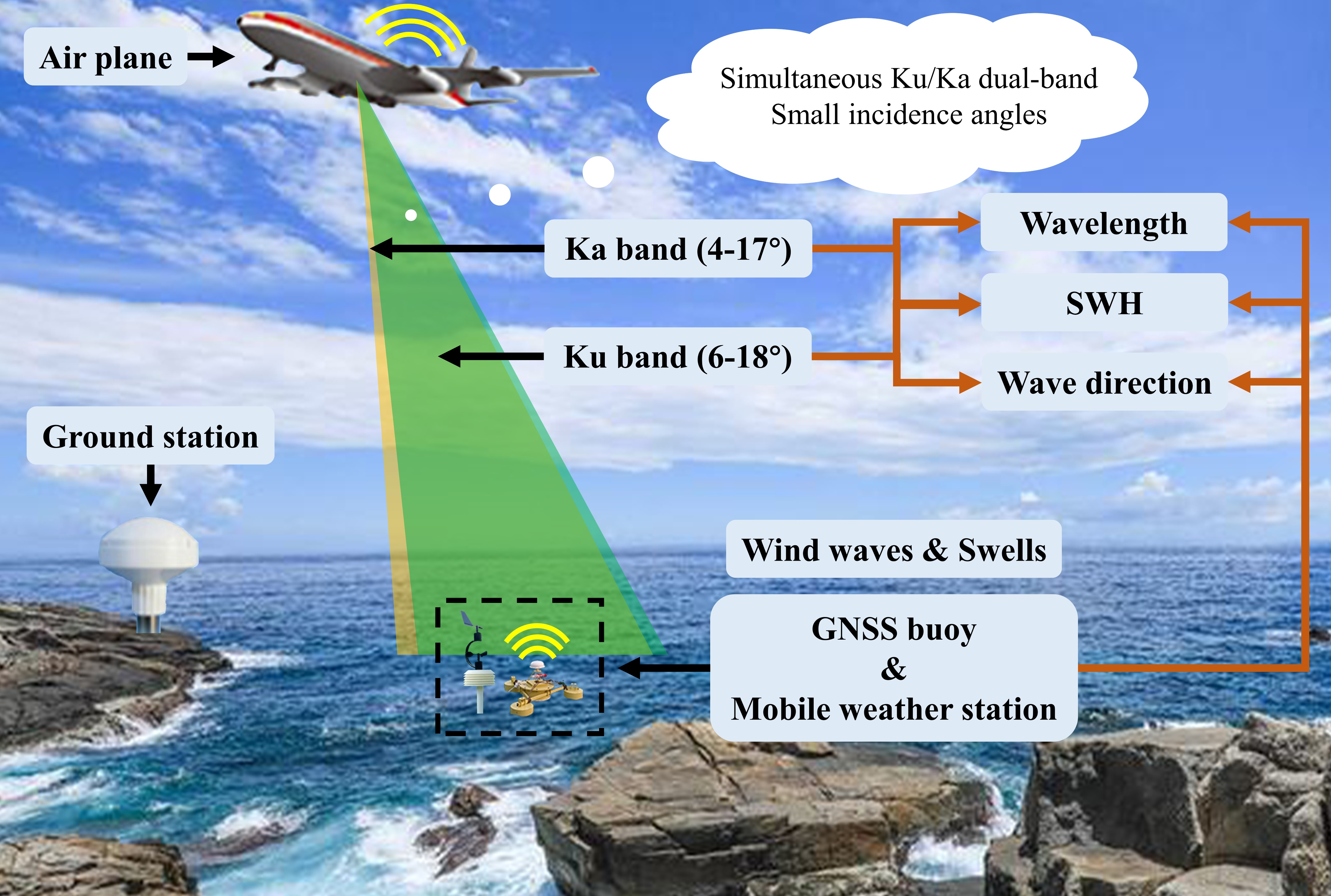
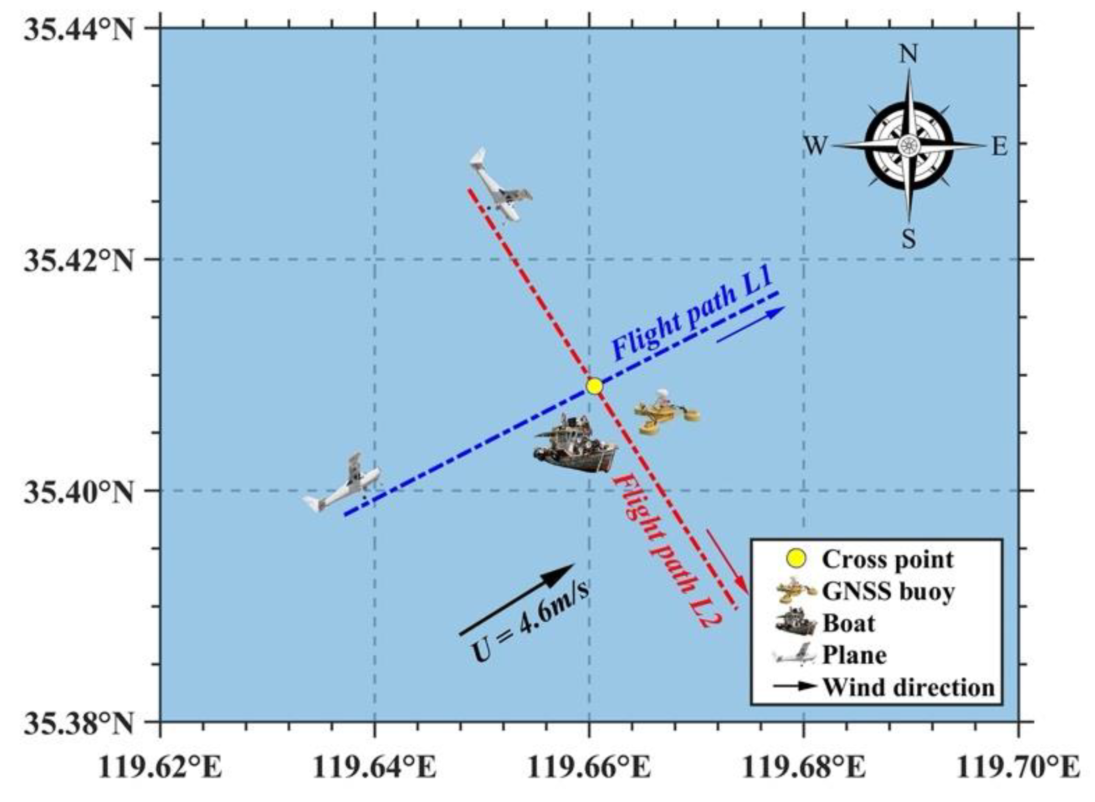
2.2. The Airborne DInIRA Observation Campaign

In order to achieve the long-distance airborne dual-band simultaneous observation, an airborne DInIRA experiment was carried out for observing the ocean waves on the sea area of Wanpingkou, Rizhao, Shandong Province, China.

As shown in Figure 2, a Global Navigation Satellite System (GNSS) buoy was placed at the intersection of the plane routes for validation purposes. The configuration parameters of the radar system and the plane are further listed in

Table 1. The main parameters of the DInIRA in this campaign.

Parameters	Frequency Band
	Ku-Band	Ka-Band
Center frequency	15.8 GHz	35.8 GHz
Baseline length	0.6 m	0.34 m
Incidence angle	6–18°	4–17°
Bandwidth	900 MHz
Sample frequency	1.2 GHz
Antenna operation mode	Single transmission and dual reception
Pulse repetition frequency	2500 Hz
Flight altitude	3.38 km
Flight velocity	68 m/s
Baseline roll angle	10°

. To assess the inversion accuracy of the OWPs in the Ku and Ka bands at small incidence angles, the incidence angle ranges were set to 6–18° (Ku) and 4–17° (Ka), respectively. It is worth noting that the sea surface targets in this incidence range are reflected mainly as specular scattering.

In addition, the sampling frequency of the in situ GNSS buoy was set to 5 Hz. Finally, the echo data of the airborne dual-band simultaneous observation and the one-dimensional (1D) 5 Hz SSH in situ data were obtained. As depicted in Figure 3a, a mobile weather station was configured on the boat to obtain environmental information such as wind speed and wind direction.

2.3. Ocean Wave Inversion

According to the data processing procedure shown in Figure 4, the echo data of the dual-band and the 1D 5 Hz SSH in situ data were processed, and the OWPs could be further extracted. Upon obtaining the OWPs from different data sources, the OWPs (in red) using the in situ data were exploited to validate the OWPs (in blue) based on the interferometric data. The SSH was established based on the World Geodetic System 1984 (WGS-84) ellipsoid surface.

The signal intensity of the single look complex (SLC) images after the SAR focusing is illustrated in Figure 5. The x-axis, here, refers to the ground-range direction, and the y-axis shows the plane flight direction. As displayed in Figure 6, the intensity images were averaged along the azimuth direction, and the result revealed that the mean signal intensity curves of the Ku and Ka bands decreased along the ground-range direction, and their intensity trends were consistent due to the adjusted incidence angles. The major reason for this trend was that the backscatter coefficient diminished and the ground range resolution declined along with the incidence angle.

In recent years, registration methods have been developed significantly [30,31,32,33]. For regions with consistent scattering characteristics and high coherence, an early study indicated that the registration accuracy of the complex-number correlation coefficient registration method was significantly better than that of the real-number registration function method [34]. In this paper, due to the consistent scattering characteristics of targets and the high coherence (Figure 7a,b) between master and slave images, the high-quality interferometric phase diagrams of the Ku and Ka bands were further calculated based on the image-based complex-number correlation algorithm, whose results are shown in Figure 7c,d.

According to Figure 7a,b, the coherences of the master and slave SLC for the Ku and Ka bands were good after the registration. The statistical results of the coherence coefficient (not displayed here) also demonstrated that ~90% of the areas could reach above 0.9 in the Ka band, indicating that the master and slave images were highly correlated in phase. In addition, the coherence coefficients of the Ku-band data were more uniformly distributed as compared with those of the Ka band, and the primary reason for this issue was that the Ku-band electromagnetic waves were less affected by the volumetric decorrelation than those of the Ka band. Figure 7c,d shows the interferometric phase diagrams of the Ku and Ka bands, respectively. Even if the interferometric phase was not filtered, the interference fringes of the dual-band data were still relatively bright, suggesting that the measured data were of high quality and the SAR-focus processing was sufficiently reliable.

The interference phases included the flat-earth phase, elevation phase, and random phase errors. In order to improve the accuracy of ocean wave inversion, the random phase errors (which can impact the SSH inversion) in the interferometric phase diagrams needed to be suppressed. Since the sea surface was relatively stable and its interference phase was uniformly distributed, the multi-look filtering algorithm could ensure the original geometry of the sea surface even in the area of unexpected phase changes. Similarly, Franceschetti et al., (2016) [35] proposed a relationship between the standard deviation of the phase noise and the multi-look numbers, establishing that the phase noise could be moderated by adding to the multi-look numbers. However, an excessive multi-look number could distort the SSH. Moreover, Sun et al., (2021) [36], in a more systematic study on the selection of multi-look numbers, suggested that an inappropriate multi-look number could cause additional random phase errors and even partly suppress the inversion of wind waves. In addition to random phase noise, an additional phase introduced by the scattering of the sea surface objects, the distribution of the flat earth phase, and the ground distance resolution, accordingly, needed to be further considered when filtering the interference phases. In this paper, a 40 × 2 multi-look window was chosen for filtering with the mean filtering algorithm, and the results are illustrated in Figure 8a.

The phase filtering significantly downgraded the effect of the random phase noise for further experiments. The flat-earth phase also needed to be removed for extracting the elevation phase (closely related to the ocean waves). In this paper, the flat-earth phase was thus removed based on the orbital data of the inertial navigation system in the plane. The interferometric phase diagram (viz. the Ka band) is shown in Figure 8a. As well, Figure 8b displays the elevation phase after removing the flat-earth effect, and the upper right part of Figure 8b represents the selected local area (i.e., the buoy area), and the ocean wave profiles, which can be clearly distinguished. The selected area is utilized for the inversion of the ocean waves.

The inversion results of the SSH in the Ku and Ka bands are shown in Figure 9. Given the incidence angle configuration, the swath of the Ka band (~800 m) was wider than that of Ku band (~700 m). In addition, the inversion results of the far range performed relatively worse as compared with the near range, due to the lower SNR. The phase error caused by the low SNR still existed after filtering, and therefore, these areas were avoided as much as possible when selecting the crossover ones. In this paper, we selected the buoy areas in the SSH inversion results of the Ku (in black box) and Ka bands (in red box) for further experiments, respectively. Noteworthy, the Ka band was more sensitive to the sea surface geometry than the Ku band, whose differences are described in Section 4.

To draw a distinction with the field instrument data, the SSH inversion results of the GNSS buoy (viz. the boxed area in Figure 9) were cropped for validation. The original SSH inversed by the DInIRA at the GNSS buoy area (grid resolution of 0.3 m × 0.3 m) is presented in Figure 10b,d. It was generally accepted that the signals with the wavelengths less than 3 m in the ocean were primarily noise signals, and that the long-period signals (might be associated with the geoid signal) could affect the inversion of ocean waves. These signals could be removed by using a band-pass filter (cut-off wavelength was set to 3–150 m). Finally, the wavelengths of 3–150 m were further retained after filtering, and the residual signals in the data were mainly the ocean waves. The results after band pass filtering are depicted in Figure 10a,c, and then exploited to retrieve the ocean waves.

3. Result

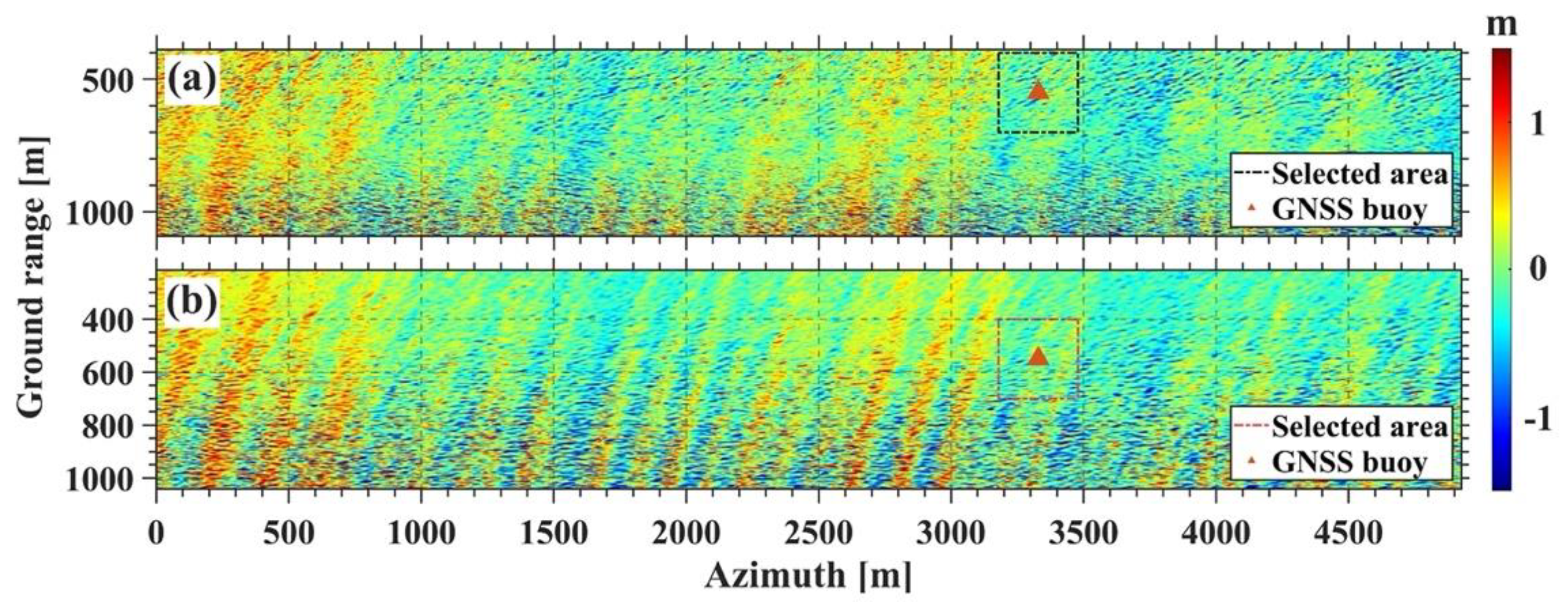
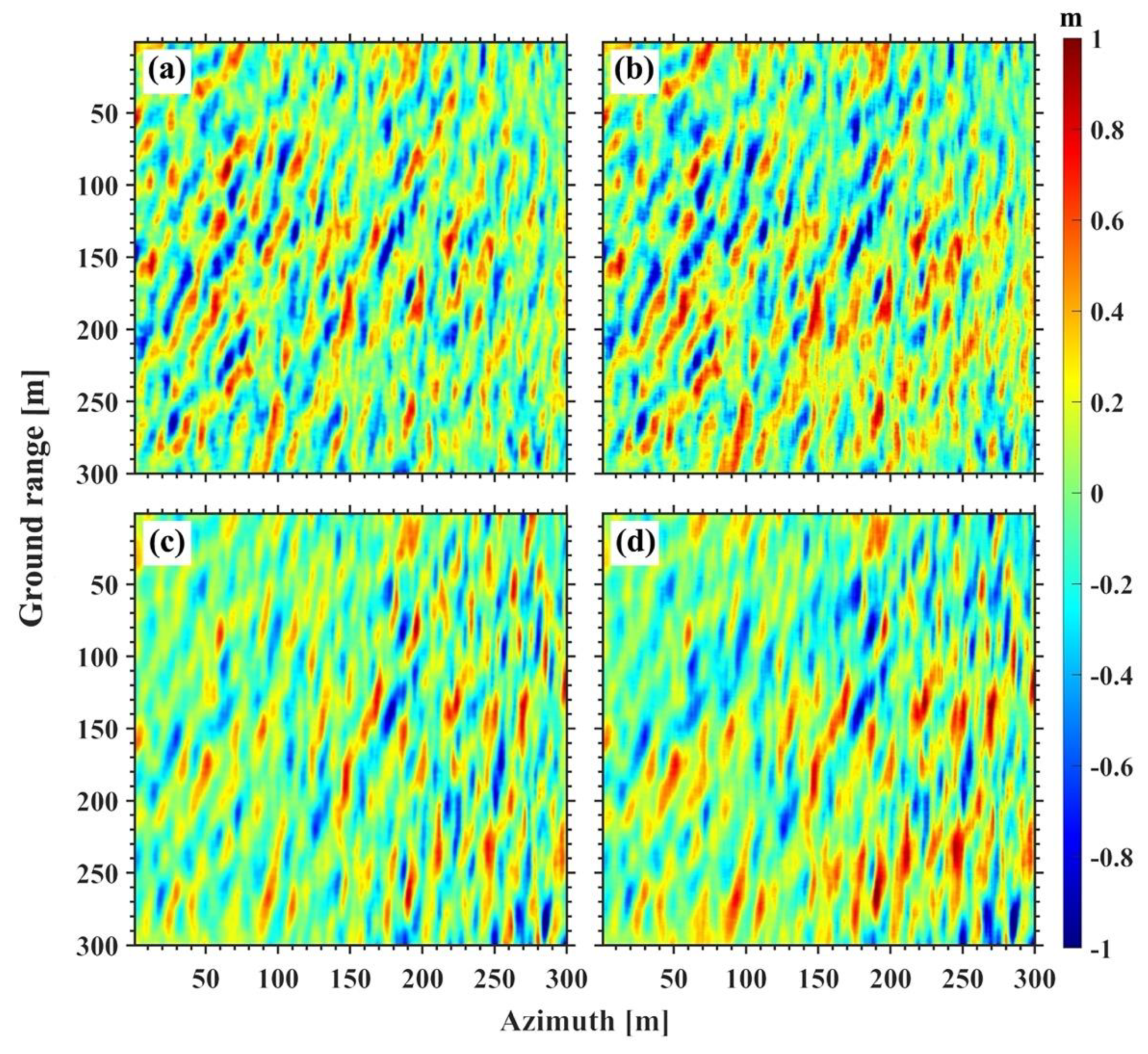
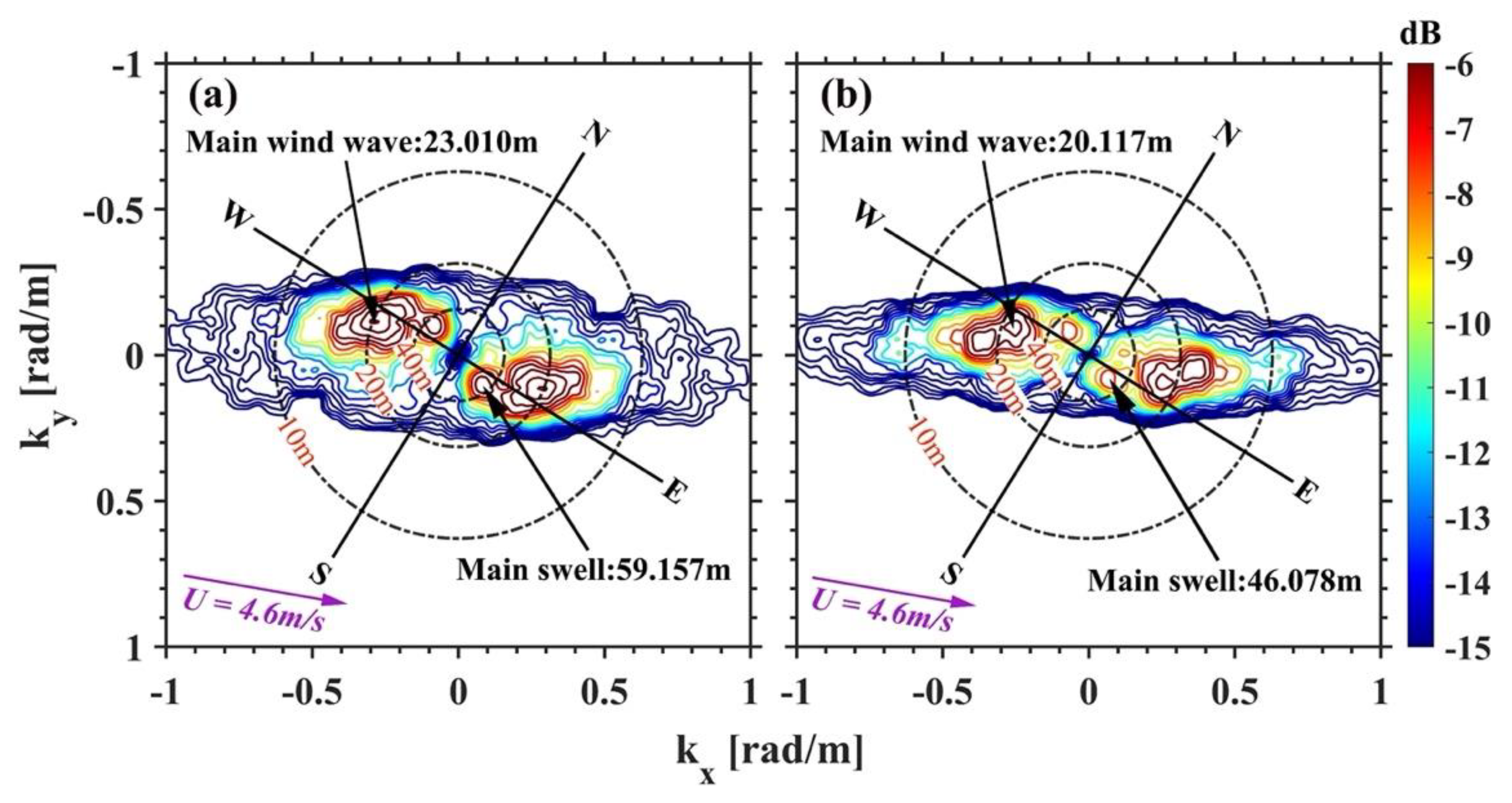
3.1. Ocean Wave Inversion Results

According to Figure 11, the 2D OWS were calculated using the $FFT2$ based on the relative SSH inversion results in the buoy area (Figure 10a,c). The high precision 2D OWS (4000 × 4000 matrix size) were obtained further by four times upsampling, after that, a 5 × 5 sliding window was used to calculate the average value of the window corresponding to each matrix element, and $k_p$ was estimated based on the coordinates ($k_x,k_y$) corresponding to the maximum value of the average matrix. The $k_x$ and $k_y$ denote the wavenumber vectors in the ground range (viz. the cross-track) and azimuth direction, respectively, and the angle in polar coordinates is in degrees clockwise to the true north direction (N). In addition, the black circles play an auxiliary role to indicate different wavelengths (i.e., 40, 20, and 10 m), and the blue circles indicate the corresponding MWW of the wind waves and swells. It can be inferred that the Ku and Ka bands had the same ability to invert the WPD in Figure 11. However, the MWW inversion results in the Ku and Ka bands showed a noticeable difference, and the MWW of the swells in the Ku band was ~13.08 m longer than the Ka band.

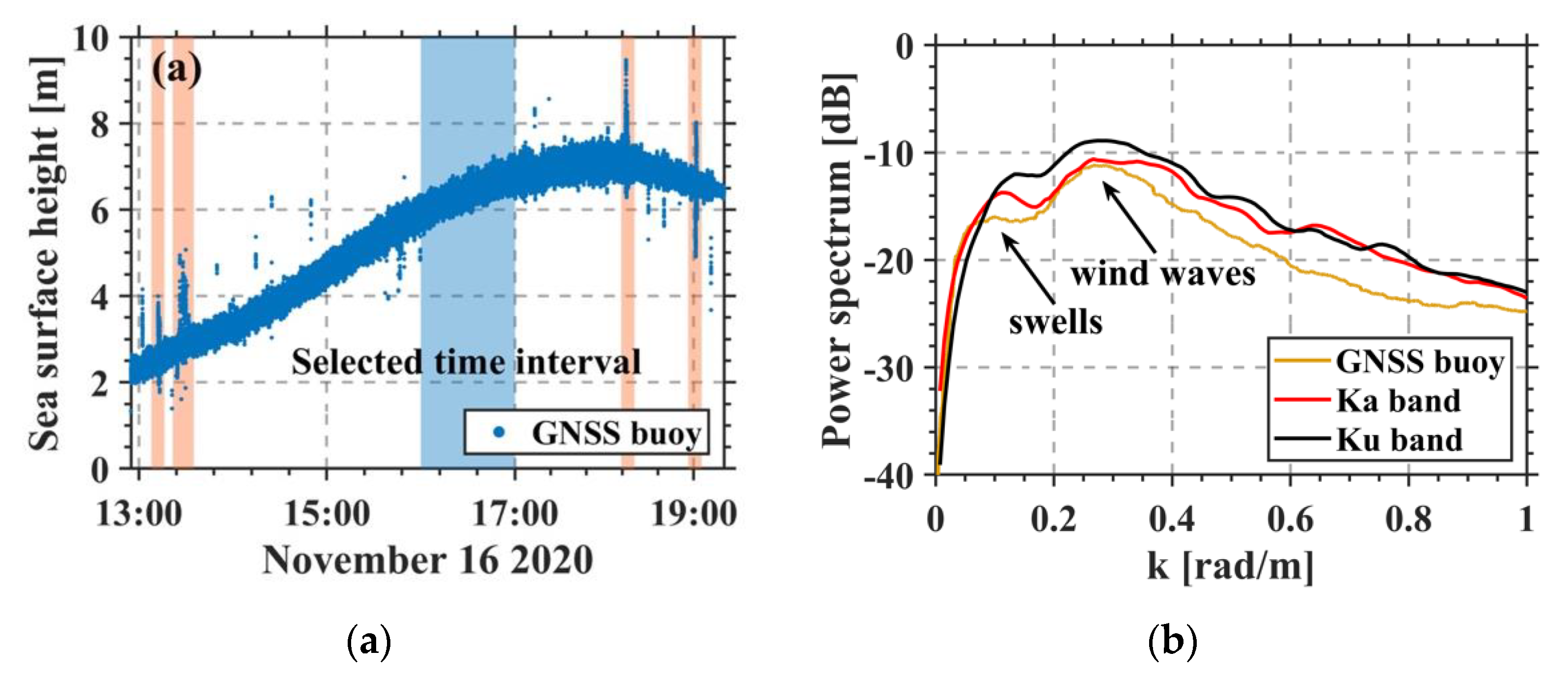
3.2. Verification Based on In situ Data

With reference to

Table 2. Inversion results of WPD based on OWS and wind direction.

Data	EWD/°	WPD/°
		Main Swell	Main Wind Wave
Mobile weather station	Southeast	-	-
Ku band	-	~105	~80
Ka band	-	~105	~80

, the WPD inversion results for the wind waves were consistent with the environmental wind direction (EWD, according to the mobile weather station), verifying the inversion accuracy of the OWS in part.

The raw data of the in situ GNSS buoy needed to be further processed for validation. The post-processing kinematic (PPK) method has been accordingly demonstrated to be an efficient technique for extracting GNSS data [37]. Thus, the PPK method was finally adopted to retrieve the 5 Hz SSH from the data acquired by the GNSS buoy. To compare it with the inversion results of the OWPs based on the echo data, the 1D SSH inversed by the buoy data used the same reference surface (viz. the WGS-84 reference ellipsoid).

The inversion results of the 1-D SSH are shown in Figure 12a. The height sequence collected by the GNSS buoy mainly contained the low frequency signals (related to the tides) and the high-frequency signals (related to the wave-induced SSH). In order to suppress the influence of the noise signals, high-frequency ocean waves signals and the boat-related signals on the ocean wave inversion, a low-pass filter was utilized (cut-off interval was set to 25 s). In addition, the influence of the long-period signals was decreased using a Butterworth high-pass filter.

Due to the complex environmental conditions of the sea surface, the collected data during 1 h (16:00–17:00) around the DInIRA imaging time was selected for validation purposes. As shown in Figure 12a, the selected time interval is indicated by the blue rectangle box, and the part with the red rectangle box is related to the towing of the ship.

The 1D relative height of the sea surface was further obtained after tidal correction, and the 1D frequency spectra $S_{buoy}\left(f\right)$ were calculated using the fast Fourier transform (FFT). The 1D OWS are accordingly obtained using the following equation [36]:

$$S_{buoy}\left(k\right)=\frac{\sqrt{g/k}{S}_{buoy}\left(f\right)}{4\pi }$$

(7)

The 1D OWS inversed by the GNSS buoy data are depicted in Figure 12b. It was inferred that the two main wave patterns (wind waves and swell waves) existed in the GNSS area. The main wave number of the swells was ~0.1 rad/m, and that of the wind waves was ~0.28 rad/m, corresponding to the ~59.16 m and ~23.01 m wavelengths, respectively. The SWH was further achieved by integrating the 1D OWS [28]:

$$\mathrm{SWH}=4.005\times \sqrt{{{\displaystyle \int }}^{ }{S}_{buoy}\left(k\right)dk}$$

(8)

In order to better compare with in situ buoy data, the 2D wavenumber spectra were converted to 1D wavenumber spectra using the following equation [36]:

$$S\left(k\right)={{\displaystyle \int }}_{-\pi }^{\pi }S\left(k\cos \phi ,k\sin \phi \right)kd\phi$$

(9)

where $S\left(k\cos \phi ,k\sin \phi \right)$ denotes the 2D wavenumber spectra, and $\phi$ is the angle with respect to the positive direction of the $k_x$ axis. The conversion results are shown in Figure 12b, and it can be seen that the 1D spectrum inversion results of the Ka band are closer to the I -situ GNSS data than those of Ku band.

The inversion results of the ocean waves based on the in situ data are outlined in

Table 3. Inversion results of SWH and MWW.

Data	SWH/m	Bias/m	MWW/m
			Swell	Bias/m	Wind Waves	Bias/m
GNSS buoy	0.69	-	62.83	-	22.44	-
Ku band	1.07	0.38	46.08	16.75	20.12	2.32
Ka band	0.96	0.27	59.16	3.67	23.01	0.57

. The inversion biases of the SWH retrieved by the Ku and Ka bands were, respectively, equal to 0.38 m and 0.27 m, the inversion biases of the MWW for the swells were 16.75 m and 3.67 m, and the inversion biases about the MWW for wind waves were 2.32 m and 0.57 m. Overall, the wind waves and swells could be effectively retrieved by the DInIRA, and the inversion accuracy (viz. the SWH and the MWW) in the Ka band outperformed the Ku band.

3.3. Accuracy Analysis of Ocean Wave Inversion Results

For the InIRA system, the altimetric accuracy could be calculated by:

$$\mathsf{\Delta }h=\frac{\lambda r_1\sin \theta }{2\pi B\cos \left(\theta -\alpha \right)}\mathsf{\Delta }\varphi$$

(10)

where $\mathsf{\Delta }h$ stands for the relative height change and $\mathsf{\Delta }\varphi$ corresponds to the phase change. Therefore, a smaller incidence angle, a longer baseline, a shorter radar wavelength, and more accurate phase difference could significantly improve the altimetric accuracy.

Since the phase was limited to [−π,π], a sizeable relative height (~6 m at near range) change led to phase ambiguity (wrapping) [38]. The altimetric ambiguity was further determined as the relative height change corresponding to the 2π phase change, and was calculated by:

$$h_{2\pi }=\frac{\lambda r_1\sin \theta }{B\cos \left(\theta -\alpha \right)}$$

(11)

The DInIRA parameters configured in this campaign were substituted into Equation (11), whose results are shown in Figure 13a, where the buoy area (viz. the inversion experiment area of the ocean waves) is indicated by the blue box. Although the Ka-band wavelength was shorter than that of the Ku band, the altimetric ambiguity could also change from 5 m (near range) to 28 m (far range) due to its short length of the baseline (0.34 m). As the SSH change was usually within a few meters, the processing procedure of the phase unwrapping could be avoided, to a large extent, with the parameter configuration of the DInIRA. However, excessive altimetric ambiguity could also bring challenges to the design of the DInIRA system. According to Figure 13b, the corresponding phase change decreased from 0.058 rad (near range) to 0.013 rad (far range) in the Ka band for a relative height change of 5 cm. The stringent requirement for phase sensitivity also required that the thermal noise of the system was limited to a certain level, and that the data processing was highly precise. As compared with the Ka band, the Ku band possessed more stringent requirements for limiting the random errors, such as the thermal noise in the near range.

An essential prerequisite for high-accuracy inversion of the SSH is a high coherence between the signals acquired by the primary and auxiliary antennas. The decorrelation factors [39,40] mainly include thermal, doppler, baseline, volumetric, time, and data processing. The doppler and baseline decorrelation can be removed by prefiltering in azimuth and range directions, respectively. The time decorrelation only needs to be considered in multi-pass measurement systems. Due to the high imaging quality of the airborne DInIRA, the height measurement error (after registration and multi-look fliting) caused by data processing decorrelation was only on the order of millimeters, and therefore, could be disregarded.

Thermal decorrelation was mainly induced by the InIRA system thermal noise [41]. Thermal noise influenced the phase error the most, and the decoherence factor ${\gamma }_n$ caused by the thermal noise could be derived as:

$${\gamma }_n=\sqrt{\frac{SN{R}_{1}SN{R}_2}{\left(1+SN{R}_1\right)\left(1+SN{R}_2\right)}}$$

(12)

where $SN{R}_1$ and $SN{R}_2$ denote the SNR of the master and the slave SLC, respectively. Of note, the SNRs of the master and slave images were estimated from the echo data.

The volumetric decorrelation was correspondingly induced by the sea surface morphology and the attenuation function of the electromagnetic wave [42,43], and the decoherence factor ${\gamma }_v$ could be derived as:

$${\gamma }_v=e^{-2{\left(\frac{2\pi {\sigma }_{h}B}{r_1\lambda \tan \theta }\right)}^2}$$

(13)

where ${\sigma }_h$ is the standard deviation of the SSH and the target scene is a Gaussian random sea surface height (can better reflect the electromagnetic characteristics).

Then, the payload parameters and the target scene (different SWH) were substituted into Equations (12) and (13), and the simulation results are shown in Figure 14. Due to the low orbit height of the aircraft and the small incidence angle of the antenna, the coherence of the primary and auxiliary antenna signals was ensured. According to Figure 14b, the influence of the volumetric decorrelation on the imaging was significant in the near range, and it decreased with SWH reductions (along the arrow direction). In addition, the influence caused by the volumetric decorrelation on the Ku band was less than that on the Ka band, due to the longer wavelength of the Ku band.

The coherence between the master and slave SLC was further expressed as the multiplication of the decorrelation factors, as follows:

$$\gamma ={\gamma }_n·{\gamma }_v$$

(14)

The coherence coefficients between the master and slave SLC for different frequency bands are illustrated in Figure 15. Here, the coefficient increased, and then decreased with the ground range, indicating that the volumetric decorrelation dominated in the near range. In addition, the coherence decreased with the ground range due to the SNR decline within the ground range.

Although the echo data acquired by the DInIRA were of high quality, a large multi-look number needed to be used in the multi-look processing to achieve high accuracy of the height measurement. It was established that the interference phase difference could be approximated with the multi-look number $WH>4$ and the coherence coefficient $\gamma >0.2$ as:

$$\mathsf{\Delta }\phi =\sqrt{\frac{1}{2WH}}\frac{\sqrt{1-{\gamma }^2}}{\gamma }$$

(15)

The simulation result of altimetric accuracy could be further calculated by substituting the calculation of Equation (15) into Equation (10). In addition, the different multi-look numbers, $N$, were performed. As shown in Figure 16a, the altimetric accuracy was improved with an increase (along the direction of the arrow) in $N$. The carrier parameters ($\lambda$, $B$, and $\alpha$) and the data processing parameter ($N=80$) were then substituted into Equation (10) for calculation, whose results (dotted line) are shown in Figure 16b. Due to the system and processing error, the theoretical altimetric accuracy was higher than the actual. Moreover, the theoretical altimetric accuracy (solid line) of the Ka band was higher than that of the Ku band when SWH = 0.7 m (according to the in situ data), and the theoretical results were generally consistent with the conclusions drawn from the field observation data. It is worth noting that the random phase noise in the Ku band remained partially residual after filtering, indicating that the Ku band was more sensitive to random noise than that of the Ka band. However, the altimetric accuracy at the far range of the Ka band was even higher than the theoretical result in the ground range of 800–1000 m, it was inferred that the distribution characteristic of the SSH was the main reason for this trend. It can be seen from Equation (10) that the inversion accuracy of this method is closely related to the SSH inversion results. In this campaign, due to the higher altimetric accuracy of the Ka band (Figure 16b), the ocean wave inversion performance of the Ka band is better than that of the Ku band.

4. Discussion

The inversion accuracy of SSH is mainly related to the quality of the observation data and the modulation effect caused by the sea surface motion. Due to the InIRA’s excellent characteristics of high SNR and high coherence at small incidence angles, the measured phase is closely related to SSH, which ensures high-quality data. However, in contrast to land, ocean waves have their unique characteristics of movement. According to the InIRA system, the primary factors [44] affecting the ocean waves inversion are velocity bunching and the layover effect. Velocity bunching can produce a substantial nonlinear effect on imaging, and the nonlinear effect is minimized when the WPD along with the ground range. In addition, the layover effect can affect the distortion of the SSH inversion results, and the influence is gradually worse with a decrease in the incidence angle. Due to the fact that the steepness of wind waves is much greater than that of swells, the primary target of the layover effect is the wind waves. Nevertheless, the effect of the layover for the wind waves is the largest when the WPD of wind waves is consistent with the cross-track direction. Sun et al., (2022) [36] estimated the maximum allowed SWH and wind speed at different incidence angles, and the result showed that the OWPs could be inversed based on the InIRA images if the incidence angle was greater than a few degrees, even under high sea state conditions. According to the field measurement data of the mobile weather station, the EWD was southeastward, and the velocity bunching had a small nonlinear effect on the imaging. Therefore, it was predicted that the OWPs could be effectively retrieved based on the DInIRA images by combining the incidence angle configurations and the EWD, which was consistent with the experimental results.

The significant factors affecting the inversion of the ocean waves are velocity bunching and the layover effect, sea surface morphology, and the payload performance. In this respect, Chen et al., (2021) [45] analyzed the altimetric accuracy of the X, Ku, and Ka bands under different sea states based on numerical simulations. The experimental results demonstrated that the dynamic wave-related errors of the InSAR altimetry were not sensitive to the frequencies but to the sea states. In other words, the sea states were not the primary reason for the discrepancy in the inversion accuracy of the ocean wave inversion in the Ku and Ka bands. As described in Section 3.3, the dual-band altimetric accuracy was analyzed to further explore the specific causes for this phenomenon, by combining the payload parameters and the sea surface morphology. When SWH = 0.7 m, the altimetric accuracy of the Ka band was higher than that of Ku band, resulting in higher inversion accuracy of the ocean waves. According to Figure 14b, the volumetric decorrelation induced by the sea surface morphology was sensitive to the frequency band. Although the effect of the volumetric decorrelation on the Ku band was not as strong as that of the Ka band, the altimetric accuracy of the Ka band was still more significant than that of the Ku band due to the baseline configuration and the extremely short wavelength of the Ka band. It can be inferred that the configuration of the payload parameters was the most effective way to improve the inversion accuracy of the ocean waves.

Since the altimetry sensitivity of the satellite-based InIRA system was higher than that of conventional satellite-based InSAR, it was concluded that ocean waves could also be well inversed using the satellite-based DInIRA images. However, the high operational altitude of the satellite could further make the DInIRA have high altimetric ambiguity. To ensure the altimetric accuracy of the DInIRA, the system noise needed to be limited by the carrier. In addition, the baseline length could be increased as much as possible while confirming the altimetric ambiguity and the phase coherence. Moreover, a longer baseline could alleviate the stringent requirement for a systematic phase noise level and data processing accuracy, allowing the DInIRA to achieve better performance. To obtain a more uniform high-accuracy inversion capability of ocean waves in a wide swath range, the distributions of the incidence angle of the Ku and Ka bands’ antennas could be adjusted.

Although the campaign topped the data limitation to some extent, it could only prove that the OWPs could be inversed well under the low sea state conditions in the Ku/Ka dual-band data. The inversion capability of the ocean waves using the airborne Ku/Ka dual-band data under the worse sea state conditions is still open to discussion. In the future, further study will focus on the data fusion using the dual-band data to improve the accuracy of ocean wave inversion, and apply this technology to the satellite altimetry.

5. Conclusions

In this study, the inversion results of ocean waves in Ku and Ka bands are compared as a first-time attempt, to the best of the authors’ knowledge, based on airborne DInIRA field observation data. Firstly, the echo data of the Ku and Ka bands are processed one by one, and the SSHs under different frequency bands are inversed based on the interference phase difference. Secondly, the 2D OWS are calculated based on the SSH inversion results and the FFT2, the OWPs are extracted from the OWS. The results show that the inversion result of WPD is consistent with the environmental wind direction. The SWH inversion biases retrieved by the Ku and Ka bands are, respectively, equal to 0.38 m and 0.27 m, the MWW inversion biases for the swells are 16.75 m and 3.67 m, and the MWW inversion biases for the wind waves are 2.32 m and 0.57 m. Overall, the swells and the wind waves can be effectively retrieved by the DInIRA, and the inversion accuracy of the SWH and the MWW in the Ka band is better than those in the Ku band. Finally, in this paper, we explained and discussed the results from the perspective of altimetric accuracy, concluding that the Ku band is more sensitive to random noise than the Ka band, which can lead to its worse inversion accuracy of ocean waves in this airborne campaign as compared with the Ka band.

Even though some of the system parameters in this airborne DInIRA campaign are limited by the payload performance and the current technical conditions, the small-angle-based DInIRA system has shown great potential in high-accuracy SSH measurement. This study additionally validated the inversion capability of ocean waves in Ku and Ka bands, which will improve the knowledge of the Ka band at small angles and provide a reference for the parameter design of the DInIRA system.

References

1. Scharroo, R.; Bonekamp, H.; Ponsard, C.; Parisot, F.; von Engeln, A.; Tahtadjiev, M.; de Vriendt, K.; Montagner, F. Jason Continuity of Services: Continuing the Jason Altimeter Data Records as Copernicus Sentinel-6. Ocean Sci. 2016, 12, 471–479. [Google Scholar] [CrossRef] [Green Version]
2. Wang, J.; Xu, H.; Yang, L.; Song, Q.; Ma, C. Cross-Calibrations of the HY-2B Altimeter Using Jason-3 Satellite During the Period of April 2019–September 2020. Front. Earth Sci. 2021, 9, 17. [Google Scholar] [CrossRef]
3. Cai, Y.; Cheng, X.; Sun, G. A Review of Development of Radar Altimeter and Its Applications. Remote Sens. Inf. 2006, 4, 74–78. [Google Scholar]
4. Macklin, J.T.; Cordey, R.A. Seasat SAR Observations of Ocean Waves. Int. J. Remote Sens. 1991, 12, 1723–1740. [Google Scholar] [CrossRef]
5. Pramudya, F.S.; Pan, J.Y.; Devlin, A.T. Estimation of Significant Wave Height of Near-Range Traveling Ocean Waves Using Sentinel-1 SAR Images. IEEE J. Sel. Top. Appl. Earth Observ. Remote Sens. 2019, 12, 1067–1075. [Google Scholar] [CrossRef]
6. Hasselmann, K.; Hasselmann, S. On the Nonlinear Mapping of An Ocean Wave Spectrum into a Synthetic Aperture Radar Image Spectrum and Its Inversion. J. Geophys. Res. Oceans. 1991, 96, 10713–10729. [Google Scholar] [CrossRef]
7. Engen, G.; Johnsen, H. SAR-ocean Wave Inversion Using Image Cross Spectra. IEEE Trans. Geosci. Remote Sens. 1995, 33, 1047–1056. [Google Scholar] [CrossRef]
8. Schuler, D.L.; Lee, J.S.; Kasilingam, D.; Pottier, E. Measurement of Ocean Surface Slopes and Wave Spectra Using Polarimetric SAR Image Data. Remote Sens. Environ. 2004, 91, 198–211. [Google Scholar] [CrossRef]
9. Caponi, E.A.; Crawford, D.R.; Yuen, H.C.; Saffman, P.G. Modulation of Radar Backscatter from the Ocean by a Bariable Surface Current. J. Geophys. Res. 1988, 93, 12249. [Google Scholar] [CrossRef]
10. Schulz-Stellenfleth, J.; Lehner, S. Ocean Wave Imaging Using an Airborne Single Pass Across-track Interferometric SAR. IEEE Trans. Geosci. Remote Sens. 2001, 39, 38–45. [Google Scholar] [CrossRef]
11. Schulz-Stellenfleth, J.; Horstmann, J.; Lehner, S.; Rosenthal, W. Sea Surface Imaging with an Across-track Inter-ferometric Synthetic Aperture Radar: The SINEWAVE Experiment. IEEE Trans. Geosci. Remote Sens. 2001, 39, 2017–2028. [Google Scholar] [CrossRef]
12. Quilfen, Y.; Chapron, B.; Bentamy, A.; Gourrion, J.; El Fouhaily, T.; Vandemark, D. Global ERS 1 and 2 and NSCAT Observations: Upwind/Crosswind and Upwind/Downwind Measurements. J. Geophys. Res.: Oceans. 1999, 104, 11459–11469. [Google Scholar] [CrossRef]
13. Jackson, F.C.; Walton, W.T.; Baker, P.L. Aircraft and Satellite Measurement of Ocean Wave Directional Spectra Using Scanning-beam Microwave Radars. J. Geophys. Res.: Oceans. 1985, 90, 987–1004. [Google Scholar] [CrossRef]
14. Rodriguez, E.; Pollard, B.; Martin, J. Wide-Swath Ocean Altimetry Using Radar Interferometry. IEEE Trans. Geosci. Remote Sens. 1999. Available online: http://hdl.handle.net/2014/17962 (accessed on 14 June 2022).
15. Fjortoft, R.; Gaudin, J.M.; Pourthie, N.; Lalaurie, J.C.; Mallet, A.; Nouvel, J.F.; Martinot-Lagarde, J.; Oriot, H.; Bor-deries, P.; Ruiz, C.; et al. KaRIn on SWOT: Characteristics of Near-Nadir Ka-Band Interferometric SAR Imagery. IEEE Trans. Geosci. Remote Sens. 2014, 52, 2172–2185. [Google Scholar] [CrossRef]
16. Ren, L.; Yang, J.; Dong, X.; Jia, Y.; Zhang, Y. Preliminary Significant Wave Height Retrieval from Interferometric Imaging Radar Altimeter Aboard the Chinese Tiangong-2 Space Laboratory. Remote Sens. 2021, 13, 2413. [Google Scholar] [CrossRef]
17. Altenau, E.H.; Pavelsky, T.M.; Moller, D.; Lion, C.; Pitcher, L.H.; Allen, G.H.; Bates, P.D.; Calmant, S.; Durand, M.; Smith, L.C. AirSWOT Measurements of River Water Surface Elevation and Slope: Tanana River, AK. Geophys. Res. Lett. 2017, 44, 181–189. [Google Scholar] [CrossRef] [Green Version]
18. Tuozzolo, S.; Lind, G.; Overstreet, B.; Mangano, J.; Fonstad, M.; Hagemann, M.; Frasson, R.P.M.; Larnier, K.; Garambois, P.A.; Monnier, J.; et al. Estimating River Discharge with Swath Altimetry: A Proof of Concept Using AirSWOT Observations. Geophys. Res. Lett. 2019, 46, 1459–1466. [Google Scholar] [CrossRef]
19. Pitcher, L.H.; Pavelsky, T.M.; Smith, L.C.; Moller, D.K.; Altenau, E.H.; Allen, G.H.; Lion, C.; Butman, D.; Cooley, S.W.; Fayne, J.V.; et al. AirSWOT InSAR Mapping of Surface Water Elevations and Hydraulic Gradients Across the Yukon Flats Basin, Alaska. Water Resour. Res. 2019, 55, 937–953. [Google Scholar] [CrossRef]
20. Altenau, E.H.; Pavelsky, T.M.; Moller, D.; Pitcher, L.H.; Bates, P.D.; Durand, M.T.; Smith, L.C. Temporal Variations in River Water Surface Elevation and Slope Captured by AirSWOT. Remote Sens. Environ. 2019, 224, 304–316. [Google Scholar] [CrossRef] [Green Version]
21. Zhao, C.; Chen, Z.; Jiang, Y.; Fan, L.; Zeng, G. Exploration and Validation of Wave-height Measurement Using Multifrequency HF radar. J. Atmos. Ocean. Technol. 2013, 30, 2189–2202. [Google Scholar]
22. Chen, G.; Tang, J.; Zhao, C.; Wu, S.; Yu, F.; Ma, C.; Xu, Y.; Chen, W.; Zhang, Y.; Liu, J.; et al. Concept Design of the "Guanlan" Science Mission: China’s Novel Contribution to Space Oceanography. Front. Mar. Sci. 2019, 6, 14. [Google Scholar] [CrossRef] [Green Version]
23. Tanelli, S.; Durden, S.L.; Im, E. Simultaneous Measurements of Ku- and Ka-band Sea Surface Cross Sections by an Airborne Radar. IEEE Geosci. Remote Sens. Lett. 2006, 3, 359–363. [Google Scholar] [CrossRef]
24. Hossan, A.; Jones, W.L. Ku- and Ka-Band Ocean Surface Radar Backscatter Model Functions at Low-Incidence Angles Using Full-Swath GPM DPR Data. Remote Sens. 2021, 13, 1569. [Google Scholar] [CrossRef]
25. Mori, S.; Polverari, F.; Mereu, L.; Pulvirenti, L.; Montopoli, M.; Pierdicca, N.; Marzano, F.S.; IEEE. Atmospheric Precipitation Impact on Synthetic Aperture Radar Imagery: Numerical Model at X and Ka Bands. In Proceedings of the IEEE International Geoscience and Remote Sensing Symposium (IGARSS), Milan, Italy, 26–31 July 2015. [Google Scholar]
26. Tonboe, R.T.; Nandan, V.; Yackel, J.; Kern, S.; Pedersen, L.T.; Stroeve, J. Simulated Ka- and Ku-band Radar Altimeter Height and Freeboard Estimation on Snow-covered Arctic Sea Ice. Cryosphere 2021, 15, 1811–1822. [Google Scholar] [CrossRef]
27. Kong, W.; Chong, J.; Tan, H. Performance Analysis of Ocean Surface Topography Altimetry by Ku-Band Near-Nadir Interferometric SAR. Remote Sens. 2017, 9, 933. [Google Scholar] [CrossRef] [Green Version]
28. Mandal, S.; Rao, S.; Raju, D.H. Ocean Wave Parameters Estimation Using Backpropagation Neural Networks. Mar. Struct. 2005, 18, 301–318. [Google Scholar] [CrossRef]
29. Shao, W.; Li, X.; Sun, J. Ocean Wave Parameters Retrieval from TerraSAR-X Images Validated Against Buoy Measurements and Model Results. Remote Sens. 2015, 7, 12815–12828. [Google Scholar] [CrossRef] [Green Version]
30. Gabriel, A.K.; Goldstein, R.M. Crossed orbit interferometry: Theory and experimental results from SIR-B. Int. J. Remote Sens. 1988, 9, 857–872. [Google Scholar] [CrossRef]
31. Lin, Q.; Vesecky, J.F. New approaches in interferometric SAR data processing. IEEE Trans. Geosci. Remote Sens. 1992, 30, 560–567. [Google Scholar] [CrossRef]
32. Stone, H.S.; Orchard, M.T.; Chang, E.C.; Martucci, S.A. A fast direct Fourier-based algorithm for subpixel registration of images. IEEE Trans. Geosci. Remote Sens. 2001, 39, 2235–2243. [Google Scholar] [CrossRef] [Green Version]
33. Yague-Martinez, N.; Rossi, C.; Lachaise, M.; Rodriguez-Gonzalez, F.; Fritz, T.; Breit, H. Interferometric processing algorithms of TANDEM-X data. In Proceedings of the 30th IEEE International Geoscience and Remote Sensing Symposium (IGARSS), Honolulu, HI, USA, 25–30 June 2010. [Google Scholar]
34. Bamler, R. Interferometric stereo radargrammetry: Absolute height determination from ERS-ENVISAT interferograms. In Proceedings of the IEEE International Geoscience and Remote Sensing Symposium, Honolulu, HI, USA, 24–28 July 2000. [Google Scholar]
35. Franceschetti, G.; Lanari, R. Synthetic Aperture Radar Processing, 2nd ed.; CRC Press, Inc.: Boca Raton, FL, USA, 2016. [Google Scholar]
36. Sun, D.; Zhang, Y.; Wang, Y.; Chen, G.; Sun, H.; Yang, L.; Bai, Y.; Yu, F.; Zhao, C. Ocean Wave Inversion Based on Airborne IRA Images. IEEE Trans. Geosci. Remote Sens. 2022, 60, 13. [Google Scholar] [CrossRef]
37. Yang, L.; Xu, Y.; Zhou, X.; Zhu, L.; Yu, F. Calibration of an Airborne Interferometric Radar Altimeter over the Qingdao Coast Sea, China. Remote Sens. 2020, 12, 1651. [Google Scholar] [CrossRef]
38. Rodriguez, E.; Martin, J.M. Theory and Design of Interferometric Synthetic Aperture Radars. IEE Proc. F Radar Signal Process. 1992, 139, 147–159. [Google Scholar] [CrossRef]
39. Hanssen, R.F. Radar Interferometry Data Interpretation and Error Analysis; Kluwer Academic Publishers: Dordrecht, The Netherland, 2001. [Google Scholar]
40. Zebker, H.A.; Villasenor, J. Decorrelation in Interferometric Radar Echoes. IEEE Trans. Geosci. Remote Sens. 1992, 30, 950–959. [Google Scholar] [CrossRef] [Green Version]
41. Just, D.; Bamler, R. Phase Statistics of Interferograms with Applications to Synthetic Aperture Radar. Appl. Optics. 1994, 33, 4361–4368. [Google Scholar] [CrossRef]
42. Treuhaft, R.N.; Madsen, S.R.N.; Moghaddam, M.; Van Zyl, J.J. Vegetation Characteristics and Underlying Topography from Interferometric Radar. Radio Sci. 1996, 31, 1449–1485. [Google Scholar] [CrossRef]
43. Krieger, G.; Fiedler, H.; Zink, N.; Hajnsek, I.; Younis, M.; Huber, S.; Bachmann, M.; Gonzalez, J.H.; Werner, M.; Moreira, A.; et al. The TanDEM-X mission: A Satellite Formation for High-resolution SAR Interferometry. In Proceedings of the 4th European Radar Conference, Munich, Germany, 10–12 October 2007. [Google Scholar]
44. Bai, Y.; Wang, Y.; Zhang, Y.; Zhao, C.; Chen, G. Impact of Ocean Waves on Guanlan’s IRA Measurement Error. Remote Sens. 2020, 12, 1534. [Google Scholar] [CrossRef]
45. Chen, Y.; Huang, M.; Zhang, Y.; Wang, C.; Duan, T. An Analytical Method for Dynamic Wave-Related Errors of Interferometric SAR Ocean Altimetry under Multiple Sea States. Remote Sens. 2021, 13, 986. [Google Scholar] [CrossRef]
Figure 1. Principle of height measurement (DInIRA).
Remotesensing 14 03578 g001
Figure 2. Map of the airborne experiment at Rizhao.
Remotesensing 14 03578 g002
Figure 3. (a) Mobile weather station; (b) GNSS buoy.
Remotesensing 14 03578 g003
Figure 4. Flowchart of ocean waves inversion and verification.
Remotesensing 14 03578 g004
Figure 5. Signal intensity of the master image in: (a) The Ku band; (b) the Ka band.
Remotesensing 14 03578 g005
Figure 6. Mean signal intensity curves with the ground range direction for DInIRA.
Remotesensing 14 03578 g006
Figure 7. Coherence coefficient map in: (a) The Ku band; (b) the Ka band. Interference phase diagram in: (c) The Ku band; (d) the Ka band.
Remotesensing 14 03578 g007
Figure 8. (a) Interference phase (Ka band); (b) elevation phase removed the flat earth phase and local area magnification.
Remotesensing 14 03578 g008
Figure 9. Inversion result of SSH in: (a) The Ku band; (b) the Ka band.
Remotesensing 14 03578 g009
Figure 10. The relative SSH of the GNSS buoy area by the DInIRA. The band pass filtering results of the Ku band: (a) after processing (b) before processing. The band pass filtering results of the Ka band: (c) after processing; (d) before processing.
Remotesensing 14 03578 g010
Figure 11. Inversion results of OWS in: (a) The Ku band; (b) the Ka band.
Remotesensing 14 03578 g011
Figure 12. (a) Data of GNSS buoy (5 Hz); (b) inversion result of 1D power spectra.
Remotesensing 14 03578 g012
Figure 13. (a) Altimetric ambiguity of DInIRA; (b) Altimetric sensitivity of DInIRA corresponds to a 5 cm height change.
Remotesensing 14 03578 g013
Figure 14. (a) Thermal decorrelation coefficient; (b) volumetric decorrelation coefficient.
Remotesensing 14 03578 g014
Figure 15. Theoretical correlation coefficient when SWH = 0.7 m.
Remotesensing 14 03578 g015
Figure 16. (a) Variation curves of the altimetric accuracy with the ground range direction for different multi-look numbers when SWH = 0.7 m; (b) theoretical (solid line) and actual (dotted line) altimetric accuracy when SWH = 0.7 m.
Remotesensing 14 03578 g016