Technical Note

SVASeg: Sparse Voxel-Based Attention for 3D LiDAR Point Cloud Semantic Segmentation

1
National Key Laboratory of Science and Technology on Multi-Spectral Information Processing, School of Artificial Intelligence and Automation, Huazhong University of Science and Technology, Wuhan 430074, China
2
School of Biomedical Engineering, South-Central University for Nationalities, Wuhan 430074, China
*
Author to whom correspondence should be addressed.
Remote Sens. 2022, 14(18), 4471; https://doi.org/10.3390/rs14184471
Submission received: 4 August 2022 / Revised: 5 September 2022 / Accepted: 6 September 2022 / Published: 7 September 2022
(This article belongs to the Special Issue Semantic Segmentation Algorithms for 3D Point Clouds)

Abstract

:
3D LiDAR has become an indispensable sensor in autonomous driving vehicles. In LiDAR-based 3D point cloud semantic segmentation, most voxel-based 3D segmentors cannot efficiently capture large amounts of context information, resulting in limited receptive fields and limiting their performance. To address this problem, a sparse voxel-based attention network is introduced for 3D LiDAR point cloud semantic segmentation, termed SVASeg, which captures large amounts of context information between voxels through sparse voxel-based multi-head attention (SMHA). The traditional multi-head attention cannot directly be applied to the non-empty sparse voxels. To this end, a hash table is built according to the incrementation of voxel coordinates to lookup the non-empty neighboring voxels of each sparse voxel. Then, the sparse voxels are grouped into different groups, and each group corresponds to a local region. Afterwards, position embedding, multi-head attention and feature fusion are performed for each group to capture and aggregate the context information. Based on the SMHA module, the SVASeg can directly operate on the non-empty voxels, maintaining a comparable computational overhead to the convolutional method. Extensive experimental results on the SemanticKITTI and nuScenes datasets show the superiority of SVASeg.

1. Introduction

Scene perception is a very crucial task in computer vision which has a wide range of applications (e.g., autonomous driving and robotics). LiDAR is an indispensable device in modern autonomous driving vehicles. It captures precise and far distance measurements of the environments surrounding conventional visual cameras. The obtained measurements naturally form a 3D point cloud, which can be used to identify and locate dynamic objects and drivable areas. Therefore, LiDAR point cloud semantic segmentation is a crucial task for autonomous driving, which assigns a special semantic label for each point and provides point-wise perception information of the overall scene.
Previous LiDAR segmentation approaches can be roughly grouped into four main categories: point-based, projection-based, voxel-based and multi-view fusion-based methods. Point-based approaches [1,2,3,4,5,6] directly operate on point clouds and predict the semantic label of each point. Those methods generally apply point-based operators [5,7,8,9] (e.g., sampling, grouping and ordering) to extract semantic features from raw point clouds, but they are limited to adapting to the outdoor point cloud under the property of varying density and large range of scenes, and the large number of points also results in computational difficulties. Projection-based methods [10,11,12,13] project the LiDAR point clouds into a 2D space (e.g., range image and bird-eye-view images) so that 2D convolutions can be used to process them. However, those projection-based methods cannot completely model the geometric information because the original topology will inevitably be lost or altered during the 3D-to-2D projection process.
Voxel-based methods [14,15] rasterize LiDAR point clouds into voxels and then apply 3D convolutions to extract features. Those methods are computational expensive and entail high memory consumption. Recently, more efficient sparse convolutions [16,17,18] have been proposed to accelerate 3D convolution and can achieve state-of-the-art segmentation performance. Multi-view fusion-based methods [17,19,20] combine multiple different operations (i.e., voxel-based, projection-based and/or point-wise operations) to segment point clouds, and show promising results.
Sparse convolution is a crucial operation in most segmentation models [20,21] that include voxel-based operation. Although these models have the advantage of efficiency, they cannot efficiently capture large amounts of context information, resulting in limited receptive fields and unsatisfactory performance. The receptive field of sparse convolution is related to voxel size, kernel size, stride size and layers. When trading off performance and resource consumption, it is difficult to directly increase these parameters to obtain larger receptive fields. Compared with convolutional neural networks, the transformer has showed its superiority and achieved promising results in most 2D vision tasks [22,23] and 3D object detection [24,25], because it can model the long-range relationships between pixels by self-attention and multi-head attention.
Motivated by above findings and inspired by VoTr [24] for 3D object detection, a sparse voxel-based attention network is proposed for LiDAR semantic segmentation (SVASeg). The SVASeg is mainly composed of multiple submanifold sparse convolution layers, multiple sparse inverse convolution layers and a sparse, voxel-based multi-head attention module (SMHA). For the key component, SMHA, according to the increment of voxel coordinates, a hash table is built to lookup the non-empty neighbor voxels for each voxel. Then, all sparse voxels can be grouped into different local groups. For each group, we perform position embedding, multi-head attention and feature fusion to capture the context information and enlarge the receptive fields. The SMHA only focuses on the non-empty voxels in a local region and maintains a comparable computational overhead to the convolutional method. Experimental results on SemanticKITTI and nuScenes datasets showed the superiority of SVASeg.

2. Related Work

In this section, we briefly review existing works related to our approach: LiDAR semantic segmentation and the transformer for point clouds. We mainly focus on the LiDAR-only methods.

2.1. LiDAR Semantic Segmentation

As the public datasets [26,27] of outdoor scenes increase in size and number, LiDAR semantic segmentation research is developing. These methods are grouped into four categories, including point-based, projection-based, voxel-based and multi-view fusion-based methods.
Point-based methods directly learn the point features based on the raw point clouds through point-based operators [5,7,8,9] (e.g., sampling, grouping and ordering). KPConv [5] uses kernel point convolution which utilizes kernel-points to convolve local point sets. ASAP-Net [28] designs a flexible module as soon as possible to improve spatio-temporal point cloud feature learning by considering both attention and structure information across frames. PointASNL [29] proposes an adaptive sampling module to re-weight the neighbors around the initial sampled points via farthest point sampling. S-BKI [30] develops a Bayesian, continuous 3D semantic occupancy map of point clouds by generalizing the Bayesian kernel inference model. PointNL [31] aims to build the long-range dependencies of point clouds from the neighborhood-level, superpoint-level and global-level. To capture and represent implicit geometric structures of point cloud, STPC [32] introduces a spatial direction dictionary to learn those latent geometric components and designs a sparse deformer to transform unordered neighbor points into the canonical ordered dictionary space by using direction dictionary learning. RandLA-Net [1] introduces a lightweight architecture for large-scale point clouds by using random sampling instead of complex sampling approaches. Based on RandLA-Net, MSAAN [33] proposes a multi-scale attentive aggregation network to achieve the global consistency of point cloud feature representation. However, these methods which mainly focus on indoor point cloud are limited to adapting to the outdoor point cloud under the conditions of varying density and a large range of scenes, and the large number of points also results in the computational difficulties for these methods when shifting from indoor to outdoor settings.
Projection-based methods project the input point clouds to a 2D pseudo-image. Then, a 2D convolutional neural network is used to process the pseudo-image. RangeNet++ [34], SqueezeSegV3 [11], TemporalLidarSeg [35], SalsaNext [10], KPRNet [12] and Lite-HDSeg [36] utilize the spherical projection mechanism to map the raw point clouds into a range image, and an encoder–decoder network is applied to the range image to obtain semantic information. For instance, to tackle the feature distribution of drastic LiDAR image changes at different image locations, SqueezeSegV3 [11] uses spatially-adaptive convolution to adopt different filters for different locations according to the input image. SalsaNext [10] introduces a new context module, consisting of a residual dilated convolution stack fusing receptive fields at various scales, for the uncertainty-aware semantic segmentation of a LiDAR point cloud. Lite-HDSeg [36] is a new encoder–decoder architecture with light-weight harmonic dense convolutions as its core. PolarNet [13] projects the raw point cloud into a polar bird’s-eye view (BEV). However, the original topology of point clouds will inevitably be lost or altered during projection, resulting in projection-based methods failing to completely model the geometric information.
Voxel-based methods rasterize the raw point clouds into voxels, and then apply vanilla 2D or 3D convolutions to generate LiDAR semantic segmentation results. Recently, more efficient works [16,17] have been proposed to accelerate the 3D convolution and reduce the memory consumption. Following the previous works [16,17], MinkNet42 [21] and PCSCNet [37] achieved better semantic segmentation results on outdoor scenarios. Among them, PCSCNet [37] is a fast semantic segmentation model based on the voxel-based point convolution and 3D sparse convolution. Furthermore, Cylinder3D [18] groups the raw point cloud into the cylindrical partitions and designs an asymmetrical residual block to further reduce computation and improve the segmentation performance.
Multi-view fusion-based methods construct the LiDAR segmentation model by using the combination of voxel-based, projection-based and/or point-wise operations. To capture richer semantic information, some methods [15,19,38,39,40,41,42] fuse two or more different views together. For instance, [39,40] fused the point-wise semantic information from a bird’s-eye view and a range image in the early stage, and then fed it into a 3D detector to obtain the detection results. AMVNet [38] fuses the outputs of different views in a late stage. PVCNN [15] and FusionNet [41] utilize point–voxel fusion strategies to achieve better LiDAR segmentation performance. However, the performances of these methods are also limited due to the lack of rich contextual information.

2.2. Transformer in Point Cloud

A transformer can model the long-range relationships between pixels by self-attention and multi-head attention. It has achieved promising results in most 2D vision tasks [22,23,43] and in 3D object detection [24,25]. As for 3D semantic segmentation, some works [44,45,46,47] applied the point-based transformer to point clouds for indoor scene semantic segmentation. However, these methods cannot be used for outdoor LiDAR segmentation due to the inherent properties of LiDAR points (e.g., sparsity and varying density). STPC [32] uses spatial transformer point convolution to tackle the semantic segmentation of both indoor and outdoor scenes, but its segmentation performance is unsatisfactory.

3. Proposed Method

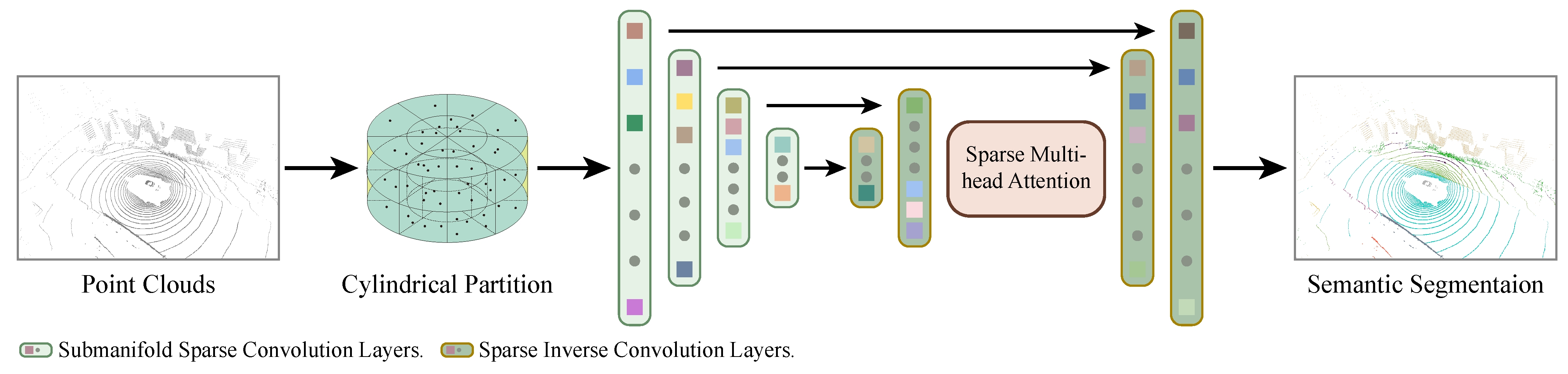
3.1. Network Architecture

In this section, we describe the whole network architecture of SVASeg for LiDAR point cloud semantic segmentation. As illustrated in Figure 1, the whole network is an encoder–decoder architecture which mainly contains four encoding layers, four decoding layers and a sparse voxel-based multi-head attention module. For each encoding layer, four submanifold sparse convolution layers are used to encode and down-sample the input sparse features. For the decoding layer, we firstly use four sparse inverse convolution layers to recover the spatial resolutions of the sparse features. The decoded features and corresponding encoded features are fused together by concatenation to further refine the fused features and improve its discrimination. Specially, after two successive decoding layers, a sparse voxel-based multi-head attention module (described in Section 3.2) is applied to the sparse features to capture the contextual information and enlarge the receptive fields for better LiDAR semantic segmentation.
For the whole pipeline, our SVASeg takes a LiDAR point cloud as input. Then, following the studies [18,20], the raw point clouds are transformed into a cylinder coordinate system and further voxelized into the cylindrical partitions as the input sparse features. Subsequently, the feature encoder and decoder are used to process the sparse features and generate sparse semantic features. Then, those sparse semantic features are converted to a dense cylindrical representation F d e n s e R B × C × H × W × L , where B is batch size; C denotes the number of feature dimensions; and H, W and L indicate the radius, angle and height, respectively. Finally, the point-wise semantic predictions can be obtained by applying a simple argmax operation and the voxelized inverse indexes to the dense semantic features.
During training, the classical cross-entropy loss function L c e is used to supervise the learning of our network, SVASeg. The L c e is a voxel-wise loss and used to maximize the point accuracy. Following previous works [18,20], the lovasz–softmax loss function [48] is also taken as an auxiliary loss L a u x to maximize the intersection-over-union score. Therefore, the total training loss of our network is
L l o s s = L c e + L a u x .

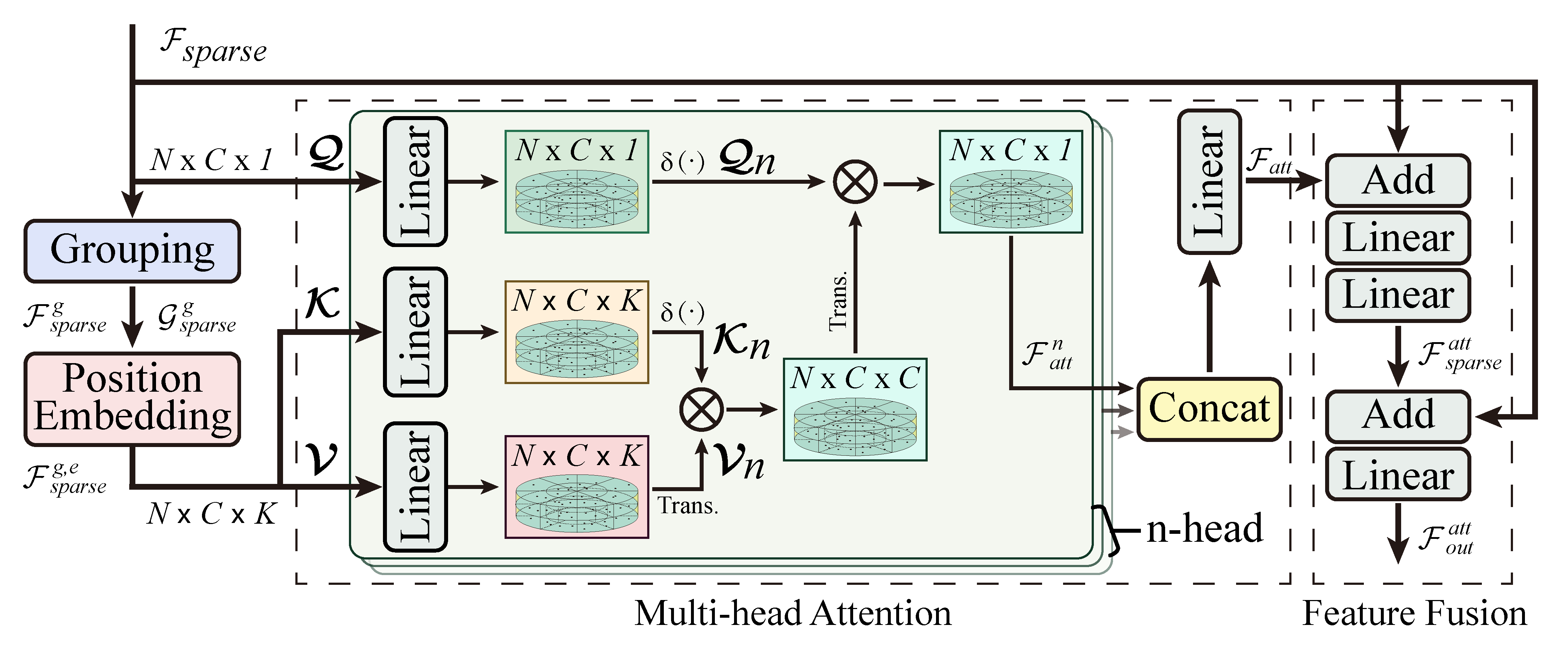
3.2. Sparse Voxel-Based Multi-Head Attention

The transformer has been widely used in various 2D vision tasks and achieves promising results, because it can build the long-range relationships between pixels by self-attention and multi-head attention. However, it is difficult to directly apply a standard tranformer module to non-empty voxels due to its sparsity. Inspired by VoTr [24] for 3D object detection, a multi-head attention module (depicted in Figure 2) is adapted to sparse non-empty voxels to capture the contextual information and enlarge the receptive fields for better LiDAR semantic segmentation.
Grouping. Given a voxel set V = { v i i = 1 , 2 , , N } with N non-empty voxels and its indices I and spatial shape S, we firstly build a hash table for each querying voxel v i according to the incrementation of voxel coordinate ( v i , x , v i , y , v i , z ) and a specific hash size K. For example, given the incrementation of voxel coordinate ( v i , x , v i , y , v i , z ) = { ( 0 , 0 , 0 ) , ( 1 , 0 , 0 ) , , ( 5 , 5 , 4 ) , ( 5 , 5 , 5 ) } , we can search K non-empty neighbor voxel indices for v i . The new indices can be obtained by ( v i , x ± v i , x , v i , y ± v i , y , v i , z ± v i , z ) , and the indices of K non-empty neighbor voxels are added into the hash table. In addition, the dimension K is also used for the position embedding. Afterwards, we can lookup the non-empty neighbor voxels V i = { v i j j = 1 , 2 , , K } from the hash table. Thus, the geometry coordinates G s p a r s e R N × 3 and the features F s p a r s e R N × C of the sparse voxels can be divided into different groups and generate G s p a r s e g R N × 3 × K and F s p a r s e g R N × C × K , respectively. Each group corresponds to a local region, and K is the number of non-empty voxels in the neighborhood of centroid voxels.
Position Embedding. In a transformer, position embedding can effectively capture the position information of each element. In this work, the relative position embedding is used because the multi-head attention will be performed in a local region. Specifically, the relative geometry coordiantes can be obtained as follows:
G s p a r s e r = G s p a r s e g ϕ G s p a r s e ,
where ϕ · extends an axis in the last of G s p a r s e . Afterwards, a linear projection function φ · is applied to the relative coordiantes G s p a r s e r to generate high-dimensional embedding features. The embedding features are further fused with the grouped sparse features:
F s p a r s e g , e = F s p a r s e g + φ G s p a r s e r .
Multi-head Attention. The multi-head attention is responsible for modeling the long-range relationships between non-empty voxels and aggregating the context information in a local region for better segmentation, which is a key component of the sparse voxel-based multi-head attention module. After getting the query features Q = φ F s p a r s e , key features K = F s p a r s e g , e and value features V = F s p a r s e g , e , Q , K and V are projected and generate corresponding multi-head features:
Q n = φ q Q , K n = φ k K , V n = φ v V ,
where φ q , φ k and φ v are the linear projection functions. n is the number of multi-head. Following the work [49], the voxel-based multi-head attention can by formulated as:
F a t t n = δ Q n d ( δ K n T d V n ) ,
where δ · is the softmax normalization function. d is the number of query feature channels. The features of all heads are fused together by using a concatenation operation and a linear fusion function φ f :
F a t t = φ f F a t t 1 , F a t t 2 , , F a t t n ,
where · is the concatenation operation. The sparse voxel-based multi-head attention is directly performed on sparse non-empty voxels, which is an efficient attention mechanism due to its extension from an approximate linear 2D transformer [49].
Feature Fusion. After aggregating the contextual information of sparse voxels by using the voxel-based multi-head attention, two shortcut connections are used to speed up the convergence of our segmentation network. Specifically, the attention features F a t t are firstly fused with the sparse features F s p a r s e by element-wise addition. Then, two linear fusion functions are applied to the fused features to refine it:
F s p a r s e a t t = φ f φ f F a t t + F s p a r s e .
Afterwards, the sparse features F s p a r s e are added with the F s p a r s e a t t , and a linear fusion function is applied to the fused features to further refine it once again and generate the final attention features F o u t a t t :
F o u t a t t = φ f F s p a r s e a t t + F s p a r s e .
The obtained attention features F o u t a t t will be further processed by the following sparse inverse convolution layers in the decoder structure.

4. Experiments

Our proposed SVASeg was evaluated on the large-scale LiDAR semantic segmentation datasets SemanticKITTI [26] and nuScenes [27] to demonstrate its effectiveness. We firstly provide a brief introduction to the dataset and evaluation metrics in Section 4.1. Then, Section 4.2 presents the implementation details of our method. Subsequently, we exhibit the detailed experiments and the comparisons with other methods on the SemanticKITTI and nuScense datasets in Section 4.3 and Section 4.4. Finally, we show ablation study experiments with various numbers of hash size in Section 4.5.

4.1. Datasets and Evaluation Metrics

The SemanticKITTI [26] dataset was collected from the KITTI Vision Benchmark and contains 22 sequences involving autonomous driving scenarios. According to the official settings, sequences from 00 to 10 should be used for training (19,130 frames) and validation (sequence 08, 4071 frames), and sequences from 11 to 21 are the test split (20,351 frames). All semantic labels on the testing split are unavailable. Each scan in the dataset contains more than 100,000 points with pointwise semantic labels of 28 classes. After merging similar categories and ignoring rare classes, a total of 19 classes remained for the task of LiDAR point cloud semantic segmentation.
The nuScenes [27] dataset is another large-scale dataset for autonomous driving which contains more than 1000 scenes collected from different areas of Boston and Singapore. This dataset has 28,130 training frames and 6019 validation frames. nuScenes provides up to 32 classes of annotations. After merging similar classes, a total of 16 classes remained for the LiDAR semantic segmentation. Furthermore, this dataset has the property of class imbalance. Specifically, cars and pedestrians are the most frequent categories, whereas bicycles and construction vehicles have limited training data. Moreover, the challenge of the nuScenes dataset also comes from the fact that it was collected at different locations and with different diverse weather conditions. Compared to the SemanticKITTI dataset, the point clouds of nuScenes are also less dense, because its sensor (Velodyne HDL-32E) has fewer beams and lower horizontal angular resolution.
Mean intersection over union ( m I o U ) is a standard evaluation metric for semantic segmentation tasks. In this work, the mIoU over all classes was taken as the evaluation metric to evaluate the LiDAR segmentation performance of our proposed approach. It can be formulated as
m I o U = 1 C i = 1 C I o U i ,
I o U i = p i i p i i + j i p i j + k i p k i ,
where p i j is the number of points that belong to class i and are predicted to be class j, and C is the number of classes.

4.2. Implementation Details

For the SemanticKITTI [26] and nuScenes [27] datasets, following the works [18,20], the LiDAR point clouds were split into cylindrical partitions with the size 480 × 360 × 32 , where three dimensions are the radius, angle and height, respectively. Then, we followed the procedure of [18] to construct a UNet-like structure [50] with submanifold sparse convolution and sparse inverse convolution. Considering the balance between segmentation performance and computation and memory consumption, we only utilized a sparse voxel-based multi-head attention module after the second decoding layer. The number of specific hash size K was set to 32, the number of n-heads was set to 4, and 256 input channels were used for the sparse multi-head attention. During the training, the proposed SVASeg was trained along with the whole framework with the ADAM optimizer with initial learning rate set to 0.001, and batch size was set to 2 for 40 epochs on a single NVIDIA RTX3090 GPU. Our proposed SVASeg was implemented based on the deep learning framework PyTorch.

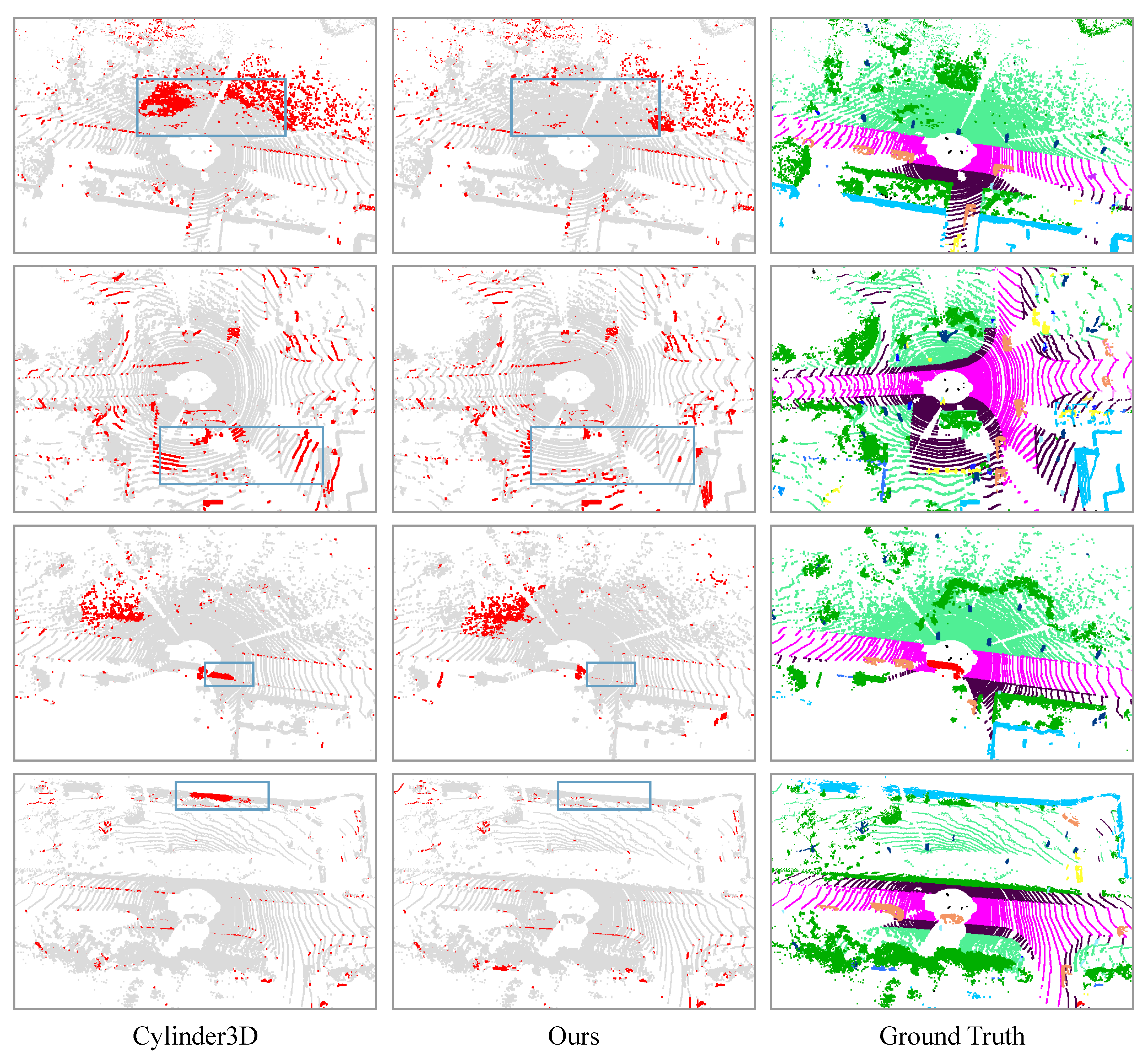
4.3. Evaluation on the SemanticKITTI Dataset

Following most previous works, we conducted experiments on SemanticKITTI [26] to evaluate the performance of our SVASeg. Table 1 reports the segmentation results of our SVASeg and other LiDAR segmentation methods on the validation set of the SemanticKITTI dataset. From Table 1, we can see that our proposed method outperforms the point-based methods (e.g., RandLANet [1]) and projection-based methods (e.g., SqueezeSegV3 [11] and SalsaNext [10]) with a large margin. Compared to the voxel-based method Cylinder3D [18], the multi-view fusion-based method AMVNet [38] and the multi-modality fusion-based method PMF [51], our approach achieved better segmentation results. Qualitative results of LiDAR segmentation are presented in Figure 3.
We also submit our segmentation results on the SemanticKITTI evaluation server. Table 2 provides the detailed class-wise quantitative results of our SVASeg and other state-of-the-art methods on the SemanticKITTI LiDAR semantic segmentation challenge. From Table 2, we can see that our proposed SVASeg achieved better segmentation performance than most state-of-the-art methods and dominated greatly in many categories. Specifically, compared to the point-based methods, including PointNL [31], STPC [32], RandLANet [1] and KPConv [5], our method outperformed the point-based methods and significantly improved the performances of LiDAR semantic segmentation. Compared to the projection-based methods, including RangeNet++ [34], SqueezeSegV3 [11], KPRNet [12], SalsaNext [10] and Lite-HDSeg [36], our proposed SVASeg achieved an about 1.4∼13.0% performance gain in terms of mIoU due to the 3D geometric information lost in projection-based methods. Compared to some voxel-based methods (e.g., PolarNet [13], MinkNet42 [21] and PCSCNet [37]) and multi-view fusion-based methods (e.g., FusionNet [41], TORANDONet [19] and SPVCNN [17]), the proposed method also performs better than these LiDAR semantic segmentation methods. The sparse voxel-based multi-head attention module is a plug-and-play module, which could be applied to other voxel-based methods to achieve further performance improvements. These results demonstrate the effectiveness and superiority of our proposed SVASeg.

4.4. Evaluation on the nuScenes Dataset

Besides evaluation on the large scale outdoor dataset SemanticKITTI [26], we also conducted experiments on another large-scale autonomous driving dataset, nuScenes [27], to further evaluate the performance of our method. Table 3 reports the LiDAR semantic segmentation results on the validation set of nuScenes. RangeNet++ [34] and Salsanext [10] use KNN as post-processing to further improve the LiDAR segmentation performance. From Table 3, we can see that our SVASeg achieves better performance than other LiDAR segmentation methods. Specifically, the proposed method outperforms the state-of-the-art projection-based methods (e.g., RangeNet++ and Salsanext) by about 6∼12% mIoU. Compared to ( A F ) 2 -S3Net [55], PolarNet [13] and Cylinder3D [18], SVASeg achieved 11.5 mIoU, 2.7 mIoU and 1.1 mIoU performance gains, respectively. Compared to the SemanticKITTI dataset, the points in the nuScenes dataset are very sparse (35k points/frame), especially bicycles, traffic-cones, etc. Therefore, the LiDAR segmentation task is more challenging. From Table 3, we can see that our proposed SVASeg also shows its effectiveness in those sparse categories.

4.5. Ablation Studies

In this sub-section, we show ablation experiments on the validation set of SemanticKITTI [26] to investigate the effect of different hash size K for grouping in the sparse voxel-based multi-head attention (SMHA) module. For a fairer and clearer comparison, we used the same configuration as in Section 4.2 for all models. Detailed experiment results are presented in Table 4. We first removed the SMHA module from SVASeg, which was taken as our baseline method. It achieved 65.2 mIoU on the validation set of SemanticKITTI. From Table 4, we can see that increasing the specific hash size K can improve the LiDAR segmentation performance, which indicates the SMHA can capture richer context information and enlarge the receptive fields for better segmentation. We also incorporated the proposed SMHA with Cylinder3D for LiDAR semantic segmentation. From Table 4, it can be observed that SMHA can effectively improve the segmentation performance, demonstrating the effectiveness of our SMHA.
Table 5 illustrates a comparison of the memory consumption, model size, time performance and performance on the validation set of the SemanticKITTI dataset. All experiments were conducted on a single GTX 3090Ti GPU with the same environment. Note that the time unit is milliseconds, and the memory and model size units are MB. Compared with the baseline model, the SHMA module only added 108 M memory consumption, 2 M parameters and 8 ms running time, which shows the SMHA maintains a comparable computational overhead to the convolutional method.

5. Conclusions

In this paper, a sparse voxel-based attention network was proposed for 3D LiDAR point cloud semantic segmentation (SVASeg). SVASeg mainly consists of four encoding layers, four decoding layers and a sparse voxel-based multi-head attention module. The encoding and decoding layers are implemented by using the submanifold sparse convolution and sparse inverse convolution, respectively, which are used to learn high-level semantic features from the input sparse voxels. The sparse voxel-based multi-head attention module is used to enlarge the receptive fields and capture rich contextual information for better segmentation, which only focuses on the non-empty voxel positions in a given local region. Extensive experimental results on the SemanticKITTI and nuScenes datasets showed the effectiveness and superiority of our SVASeg. In the future, the shift window-based transformer can be applied to SVASeg to further reduce the computational consumption and improve the performance of LiDAR semantic segmentation.

Author Contributions

Conceptualization, L.Z., L.L. and W.T.; methodology, L.Z. and S.X.; software, L.Z. and D.M.; validation, L.Z., S.X., W.T. and D.M.; writing—original draft preparation, L.Z. and S.X.; writing—review and editing, L.Z., S.X., L.L. and W.T.; supervision, W.T. and L.L.; project administration, W.T. All authors have read and agreed to the published version of the manuscript.

Funding

This work was supported by the National Natural Science Foundation of China (Grant 61976227 and 62176096).

Data Availability Statement

Not applicable.

Acknowledgments

The authors are grateful to the editor and reviewers for their constructive comments, which significantly improved this work.

Conflicts of Interest

The authors declare no conflict of interest.

References

  1. Hu, Q.; Yang, B.; Xie, L.; Rosa, S.; Guo, Y.; Wang, Z.; Trigoni, N.; Markham, A. Randla-net: Efficient semantic segmentation of large-scale point clouds. In Proceedings of the IEEE Conference on Computer Vision and Pattern Recognition, Seattle, WA, USA, 13–19 June 2020; pp. 11108–11117. [Google Scholar]
  2. Liu, L.; Yu, J.; Tan, L.; Su, W.; Zhao, L.; Tao, W. Semantic Segmentation of 3D Point Cloud Based on Spatial Eight-Quadrant Kernel Convolution. Remote Sens. 2021, 13, 3140. [Google Scholar] [CrossRef]
  3. Xu, T.; Gao, X.; Yang, Y.; Xu, L.; Xu, J.; Wang, Y. Construction of a Semantic Segmentation Network for the Overhead Catenary System Point Cloud Based on Multi-Scale Feature Fusion. Remote Sens. 2022, 14, 2768. [Google Scholar] [CrossRef]
  4. Zhao, L.; Tao, W. JSNet: Joint Instance and Semantic Segmentation of 3D Point Clouds. Proc. Aaai Conf. Artif. Intell. 2020, 34, 12951–12958. [Google Scholar] [CrossRef]
  5. Thomas, H.; Qi, C.R.; Deschaud, J.E.; Marcotegui, B.; Goulette, F.; Guibas, L.J. KPConv: Flexible and Deformable Convolution for Point Clouds. In Proceedings of the IEEE International Conference on Computer Vision, Seoul, Korea, 27 October 2019–2 November 2019. [Google Scholar]
  6. Ballouch, Z.; Hajji, R.; Poux, F.; Kharroubi, A.; Billen, R. A Prior Level Fusion Approach for the Semantic Segmentation of 3D Point Clouds Using Deep Learning. Remote Sens. 2022, 14, 3415. [Google Scholar] [CrossRef]
  7. Qi, C.R.; Yi, L.; Su, H.; Guibas, L.J. Pointnet++: Deep hierarchical feature learning on point sets in a metric space. In Proceedings of the Advances in Neural Information Processing Systems, Long Beach, CA, USA, 4–9 December 2017. [Google Scholar]
  8. Wu, W.; Qi, Z.; Fuxin, L. PointConv: Deep Convolutional Networks on 3D Point Clouds. In Proceedings of the IEEE Conference on Computer Vision and Pattern Recognition, Long Beach, CA, USA, 15–20 June 2019. [Google Scholar]
  9. Gao, F.; Yan, Y.; Lin, H.; Shi, R. PIIE-DSA-Net for 3D Semantic Segmentation of Urban Indoor and Outdoor Datasets. Remote Sens. 2022, 14, 3583. [Google Scholar] [CrossRef]
  10. Cortinhal, T.; Tzelepis, G.; Aksoy, E.E. SalsaNext: Fast, uncertainty-aware semantic segmentation of LiDAR point clouds. In Proceedings of the International Symposium on Visual Computing, San Diego, CA, USA, 5–7 October 2020; pp. 207–222. [Google Scholar]
  11. Xu, C.; Wu, B.; Wang, Z.; Zhan, W.; Vajda, P.; Keutzer, K.; Tomizuka, M. Squeezesegv3: Spatially-adaptive convolution for efficient point-cloud segmentation. In Proceedings of the European Conference on Computer Vision, Glasgow, UK, 23–28 August 2020; pp. 1–19. [Google Scholar]
  12. Kochanov, D.; Nejadasl, F.K.; Booij, O. KPRNet: Improving projection-based LiDAR semantic segmentation. arXiv 2020, arXiv:2007.12668. [Google Scholar]
  13. Zhang, Y.; Zhou, Z.; David, P.; Yue, X.; Xi, Z.; Gong, B.; Foroosh, H. Polarnet: An improved grid representation for online lidar point clouds semantic segmentation. In Proceedings of the IEEE Conference on Computer Vision and Pattern Recognition, Seattle, WA, USA, 13–19 June 2020; pp. 9601–9610. [Google Scholar]
  14. Riegler, G.; Osman Ulusoy, A.; Geiger, A. Octnet: Learning deep 3d representations at high resolutions. In Proceedings of the IEEE Conference on Computer Vision and Pattern Recognition, Honolulu, HI, USA, 21–26 July 2017; pp. 3577–3586. [Google Scholar]
  15. Liu, Z.; Tang, H.; Lin, Y.; Han, S. Point-voxel cnn for efficient 3d deep learning. arXiv 2019, arXiv:1907.03739. [Google Scholar]
  16. Graham, B.; Engelcke, M.; van der Maaten, L. 3D Semantic Segmentation with Submanifold Sparse Convolutional Networks. In Proceedings of the IEEE Conference on Computer Vision and Pattern Recognition, Salt Lake City, UT, USA, 18–23 June 2018. [Google Scholar]
  17. Tang, H.; Liu, Z.; Zhao, S.; Lin, Y.; Lin, J.; Wang, H.; Han, S. Searching efficient 3d architectures with sparse point-voxel convolution. In Proceedings of the European Conference on Computer Vision, Glasgow, UK, 23–28 August 2020; pp. 685–702. [Google Scholar]
  18. Zhu, X.; Zhou, H.; Wang, T.; Hong, F.; Li, W.; Ma, Y.; Li, H.; Yang, R.; Lin, D. Cylindrical and asymmetrical 3d convolution networks for lidar-based perception. IEEE Trans. Pattern Anal. Mach. Intell. 2021. [Google Scholar] [CrossRef]
  19. Gerdzhev, M.; Razani, R.; Taghavi, E.; Bingbing, L. Tornado-net: Multiview total variation semantic segmentation with diamond inception module. In Proceedings of the 2021 IEEE International Conference on Robotics and Automation, Xi’an, China, 30 May–5 June 2021; pp. 9543–9549. [Google Scholar]
  20. Zhao, L.; Zhou, H.; Zhu, X.; Song, X.; Li, H.; Tao, W. LIF-Seg: LiDAR and Camera Image Fusion for 3D LiDAR Semantic Segmentation. arXiv 2021, arXiv:2108.07511. [Google Scholar]
  21. Choy, C.; Gwak, J.; Savarese, S. 4d spatio-temporal convnets: Minkowski convolutional neural networks. In Proceedings of the IEEE Conference on Computer Vision and Pattern Recognition, Long Beach, CA, USA, 15–20 June 2019; pp. 3075–3084. [Google Scholar]
  22. Liu, Z.; Lin, Y.; Cao, Y.; Hu, H.; Wei, Y.; Zhang, Z.; Lin, S.; Guo, B. Swin transformer: Hierarchical vision transformer using shifted windows. arXiv 2021, arXiv:2103.14030. [Google Scholar]
  23. Li, Z.; Wang, W.; Xie, E.; Yu, Z.; Anandkumar, A.; Alvarez, J.M.; Lu, T.; Luo, P. Panoptic SegFormer. arXiv 2021, arXiv:2109.03814. [Google Scholar]
  24. Mao, J.; Xue, Y.; Niu, M.; Bai, H.; Feng, J.; Liang, X.; Xu, H.; Xu, C. Voxel transformer for 3d object detection. In Proceedings of the IEEE International Conference on Computer Vision, Montreal, QC, Canada, 11–17 October 2021; pp. 3164–3173. [Google Scholar]
  25. Fan, L.; Pang, Z.; Zhang, T.; Wang, Y.X.; Zhao, H.; Wang, F.; Wang, N.; Zhang, Z. Embracing Single Stride 3D Object Detector with Sparse Transformer. arXiv 2021, arXiv:2112.06375. [Google Scholar]
  26. Behley, J.; Garbade, M.; Milioto, A.; Quenzel, J.; Behnke, S.; Stachniss, C.; Gall, J. Semantickitti: A dataset for semantic scene understanding of lidar sequences. In Proceedings of the IEEE International Conference on Computer Vision, Seoul, Korea, 27 October–2 November 2019; pp. 9297–9307. [Google Scholar]
  27. Caesar, H.; Bankiti, V.; Lang, A.H.; Vora, S.; Liong, V.E.; Xu, Q.; Krishnan, A.; Pan, Y.; Baldan, G.; Beijbom, O. nuScenes: A multimodal dataset for autonomous driving. In Proceedings of the IEEE Conference on Computer Vision and Pattern Recognition, Seattle, WA, USA, 13–19 June 2020; pp. 11621–11631. [Google Scholar]
  28. Cao, H.; Lu, Y.; Lu, C.; Pang, B.; Liu, G.; Yuille, A. Asap-net: Attention and structure aware point cloud sequence segmentation. arXiv 2020, arXiv:2008.05149. [Google Scholar]
  29. Yan, X.; Zheng, C.; Li, Z.; Wang, S.; Cui, S. Pointasnl: Robust point clouds processing using nonlocal neural networks with adaptive sampling. In Proceedings of the IEEE/CVF Conference on Computer Vision and Pattern Recognition, Seattle, WA, USA, 13–19 June 2020; pp. 5589–5598. [Google Scholar]
  30. Gan, L.; Zhang, R.; Grizzle, J.W.; Eustice, R.M.; Ghaffari, M. Bayesian spatial kernel smoothing for scalable dense semantic mapping. IEEE Robot. Autom. Lett. 2020, 5, 790–797. [Google Scholar] [CrossRef]
  31. Cheng, M.; Hui, L.; Xie, J.; Yang, J.; Kong, H. Cascaded non-local neural network for point cloud semantic segmentation. In Proceedings of the 2020 IEEE International Conference on Intelligent Robots and Systems, Las Vegas, NV, USA, 24 October–24 January 2020; pp. 8447–8452. [Google Scholar]
  32. Fang, Y.; Xu, C.; Cui, Z.; Zong, Y.; Yang, J. Spatial transformer point convolution. arXiv 2020, arXiv:2009.01427. [Google Scholar]
  33. Geng, X.; Ji, S.; Lu, M.; Zhao, L. Multi-scale attentive aggregation for LiDAR point cloud segmentation. Remote Sens. 2021, 13, 691. [Google Scholar] [CrossRef]
  34. Milioto, A.; Vizzo, I.; Behley, J.; Stachniss, C. Rangenet++: Fast and accurate lidar semantic segmentation. In Proceedings of the 2019 IEEE International Conference on Intelligent Robots and Systems, Macau, China, 3–8 November 2019; pp. 4213–4220. [Google Scholar]
  35. Duerr, F.; Pfaller, M.; Weigel, H.; Beyerer, J. LiDAR-based recurrent 3D semantic segmentation with temporal memory alignment. In Proceedings of the 2020 International Conference on 3D Vision, Fukuoka, Japan, 25–28 November 2020; pp. 781–790. [Google Scholar]
  36. Razani, R.; Cheng, R.; Taghavi, E.; Bingbing, L. Lite-hdseg: Lidar semantic segmentation using lite harmonic dense convolutions. In Proceedings of the 2021 IEEE International Conference on Robotics and Automation, Xi’an, China, 30 May 2021–5 June 2021; pp. 9550–9556. [Google Scholar]
  37. Park, J.; Kim, C.; Jo, K. PCSCNet: Fast 3D Semantic Segmentation of LiDAR Point Cloud for Autonomous Car using Point Convolution and Sparse Convolution Network. arXiv 2022, arXiv:2202.10047. [Google Scholar]
  38. Liong, V.E.; Nguyen, T.N.T.; Widjaja, S.; Sharma, D.; Chong, Z.J. AMVNet: Assertion-based Multi-View Fusion Network for LiDAR Semantic Segmentation. arXiv 2020, arXiv:2012.04934. [Google Scholar]
  39. Wang, Y.; Fathi, A.; Kundu, A.; Ross, D.; Pantofaru, C.; Funkhouser, T.; Solomon, J. Pillar-based object detection for autonomous driving. In Proceedings of the European Conference on Computer Vision, Glasgow, UK, 23–28 August 2020. [Google Scholar]
  40. Zhou, Y.; Sun, P.; Zhang, Y.; Anguelov, D.; Gao, J.; Ouyang, T.; Guo, J.; Ngiam, J.; Vasudevan, V. End-to-end multi-view fusion for 3d object detection in lidar point clouds. In Proceedings of the Conference on Robot Learning, PMLR, Virtual, 16–18 November 2020; pp. 923–932. [Google Scholar]
  41. Zhang, F.; Fang, J.; Wah, B.; Torr, P. Deep fusionnet for point cloud semantic segmentation. In Proceedings of the European Conference on Computer Vision, Glasgow, UK, 23–28 August 2020; pp. 644–663. [Google Scholar]
  42. Chen, K.; Oldja, R.; Smolyanskiy, N.; Birchfield, S.; Popov, A.; Wehr, D.; Eden, I.; Pehserl, J. MVLidarNet: Real-Time Multi-Class Scene Understanding for Autonomous Driving Using Multiple Views. arXiv 2020, arXiv:2006.05518. [Google Scholar]
  43. Dosovitskiy, A.; Beyer, L.; Kolesnikov, A.; Weissenborn, D.; Zhai, X.; Unterthiner, T.; Dehghani, M.; Minderer, M.; Heigold, G.; Gelly, S.; et al. An image is worth 16 × 16 words: Transformers for image recognition at scale. arXiv 2020, arXiv:2010.11929. [Google Scholar]
  44. Zhao, H.; Jiang, L.; Jia, J.; Torr, P.H.; Koltun, V. Point transformer. In Proceedings of the IEEE International Conference on Computer Vision, Montreal, QC, Canada, 10–17 October 2021; pp. 16259–16268. [Google Scholar]
  45. Mazur, K.; Lempitsky, V. Cloud transformers: A universal approach to point cloud processing tasks. In Proceedings of the IEEE International Conference on Computer Vision, Montreal, QC, Canada, 10–17 October 2021; pp. 10715–10724. [Google Scholar]
  46. Wang, J.; Chakraborty, R.; Stella, X.Y. Spatial transformer for 3D point clouds. IEEE Trans. Pattern Anal. Mach. Intell. 2021. [Google Scholar] [CrossRef] [PubMed]
  47. Guo, M.H.; Cai, J.X.; Liu, Z.N.; Mu, T.J.; Martin, R.R.; Hu, S.M. Pct: Point cloud transformer. Comput. Vis. Media 2021, 7, 187–199. [Google Scholar] [CrossRef]
  48. Berman, M.; Triki, A.R.; Blaschko, M.B. The lovász-softmax loss: A tractable surrogate for the optimization of the intersection-over-union measure in neural networks. In Proceedings of the IEEE Conference on Computer Vision and Pattern Recognition, Salt Lake City, UT, USA, 18–23 June 2018; pp. 4413–4421. [Google Scholar]
  49. Shen, Z.; Zhang, M.; Zhao, H.; Yi, S.; Li, H. Efficient attention: Attention with linear complexities. In Proceedings of the IEEE Winter Conference on Applications of Computer Vision, Waikoloa, HI, USA, 3–8 January 2021; pp. 3531–3539. [Google Scholar]
  50. Ronneberger, O.; Fischer, P.; Brox, T. U-net: Convolutional networks for biomedical image segmentation. In Proceedings of the International Conference on Medical Image Computing and Computer-Assisted Intervention, Munich, Germany, 5–9 October 2015; pp. 234–241. [Google Scholar]
  51. Zhuang, Z.; Li, R.; Jia, K.; Wang, Q.; Li, Y.; Tan, M. Perception-aware Multi-sensor Fusion for 3D LiDAR Semantic Segmentation. In Proceedings of the IEEE International Conference on Computer Vision, Montreal, QC, Canada, 10–17 October 2021; pp. 16280–16290. [Google Scholar]
  52. Rosu, R.A.; Schütt, P.; Quenzel, J.; Behnke, S. Latticenet: Fast point cloud segmentation using permutohedral lattices. arXiv 2019, arXiv:1912.05905. [Google Scholar]
  53. Li, S.; Chen, X.; Liu, Y.; Dai, D.; Stachniss, C.; Gall, J. Multi-scale interaction for real-time lidar data segmentation on an embedded platform. IEEE Robot. Autom. Lett. 2021, 7, 738–745. [Google Scholar] [CrossRef]
  54. Alonso, I.; Riazuelo, L.; Montesano, L.; Murillo, A.C. 3d-mininet: Learning a 2d representation from point clouds for fast and efficient 3d lidar semantic segmentation. IEEE Robot. Autom. Lett. 2020, 5, 5432–5439. [Google Scholar] [CrossRef]
  55. Cheng, R.; Razani, R.; Taghavi, E.; Li, E.; Liu, B. AF2-S3Net: Attentive Feature Fusion with Adaptive Feature Selection for Sparse Semantic Segmentation Network. arXiv 2021, arXiv:2102.04530. [Google Scholar]
Figure 1. The network architecture overview of our SVASeg. LiDAR point clouds are firstly voxelized into cylindrical partitions as sparse features. Then, multiple submanifold sparse convoluation layers, sparse inverse convolution layers and a sparse multi-head attention module are used to process the sparse features and generate the point-wise semantic predictions. The voxel-based sparse multi-head attention is described in Section 3.2.
Remotesensing 14 04471 g001
Figure 2. The sparse voxel-based multi-head attention. Q , K and V indicate the query features, key features and value features, respectively. N × C × K is the shape of K and V , where N, C and K indicate the number of all non-empty voxels, the feature dimension and the number of local non-empty neighbor voxels, respectively. δ · is the softmax normalization function. Trans. represents the transpose operation of a tensor in the last two dimensions. The n-head is a parameter of multi-head attention.
Remotesensing 14 04471 g002
Figure 3. Compared to Cylinder3D, our method had less error (shown in red) when recognizing the surface region on the SemanticKITTI dataset’s validation set, thanks to the voxel-based sparse multi-head attention module. Best viewed in color.
Remotesensing 14 04471 g003
Table 1. Experimental results of our proposed SVASeg and other LiDAR segmentation methods on the SemanticKITTI dataset validation set. All results were obtained from the literature. Best and second best results are bolded and underlined.
MethodsmIoUCarBicycleMotorcycleTruckOther-VehiclePersonBicyclistMotorcyclistRoadParkingSidewalkOther-GroundBuildingFenceVegetationTrunkTerrainPoleTraffic-Sign
#Points (k)-638444521014711271295214349748149676304169120391882812531764
RandLANet [1]50.092.08.012.874.846.752.346.00.093.432.773.40.184.043.583.757.373.148.027.3
RangeNet++ [34]51.289.426.548.433.926.754.869.40.092.937.069.90.083.451.083.354.068.149.834.0
SequeezeSegV3 [11]53.387.134.348.647.547.158.153.80.095.343.178.20.378.953.282.355.570.446.333.2
MinkowskiNet [21]58.595.023.950.455.345.965.682.20.094.343.776.40.087.957.687.467.771.563.543.6
SalsaNext [10]59.490.544.649.686.354.674.081.40.093.440.669.10.084.653.083.664.364.254.439.8
SPVNAS [17]62.396.544.863.159.964.372.086.00.093.942.475.90.088.859.188.067.573.063.544.3
PMF [51]63.995.447.862.968.475.278.971.60.096.443.580.50.188.760.188.672.775.365.543.0
Cylinder3D [18]64.996.461.578.266.369.880.893.30.094.941.578.01.487.550.086.772.268.863.042.1
AMVNet [38]65.295.648.865.488.754.870.886.20.095.553.983.20.1590.962.187.966.874.264.749.3
SVASeg (Ours)66.196.853.080.288.962.878.191.41.193.741.078.70.189.755.189.265.876.765.149.0
Table 2. Experimental results of our proposed SVASeg and state-of-the-art LiDAR segmentation methods on the SemanticKITTI dataset’s official leaderboard. All results were obtained from the literature or leaderboard.
MethodsmIoUCarBicycleMotorcycleTruckOther-VehiclePersonBicyclistMotorcyclistRoadParkingSidewalkOther-GroundBuildingFenceVegetationTrunkTerrainPoleTraffic-Sign
S-BKI [30]51.383.830.643.026.019.68.53.40.092.665.377.430.189.763.783.464.367.458.667.1
PointNL [31]52.292.142.637.49.820.049.257.828.390.548.372.519.081.650.278.554.562.741.755.8
RangeNet++ [34]52.291.425.734.425.723.038.338.84.891.865.075.227.887.458.680.555.164.647.955.9
LatticeNet [52]52.992.916.622.226.621.435.643.046.090.059.474.122.088.258.881.763.663.151.948.4
RandLANet [1]53.994.226.025.840.138.949.248.27.290.760.373.720.486.956.381.461.366.849.247.7
PolarNet [13]54.393.840.330.122.928.543.240.25.690.861.774.421.790.061.384.065.567.851.857.5
MinkNet42 [21]54.394.323.126.226.136.743.136.47.991.163.869.729.392.757.183.768.464.757.360.1
STPC [32]54.694.731.139.734.424.551.148.915.390.863.674.15.390.761.582.762.167.551.447.9
MINet [53]55.290.141.834.029.923.651.452.425.090.559.072.625.885.652.381.158.166.149.059.9
3D-MiniNet [54]55.890.542.342.128.529.447.844.114.591.664.274.525.489.460.882.860.866.748.056.6
SqueezeSegV3 [11]55.992.538.736.529.633.045.646.220.191.763.474.826.489.059.482.058.765.449.658.9
TemporalLidarSeg [35]58.294.150.045.728.137.156.847.39.291.760.175.927.089.463.383.964.666.853.660.5
KPConv [5]58.896.032.042.533.444.361.561.611.888.861.372.731.695.064.284.869.269.156.447.4
SalsaNext [10]59.591.948.338.638.931.960.259.019.491.763.775.829.190.264.281.863.666.554.362.1
FusionNet [41]61.395.347.537.741.834.559.556.811.991.868.877.130.892.569.484.569.868.560.466.5
PCSCNet [37]62.795.748.846.236.440.655.568.455.989.160.272.423.789.364.384.268.268.160.563.9
KPRNet [12]63.195.554.147.923.642.665.965.016.593.273.980.630.291.768.485.769.871.258.764.1
TORANDONet [19]63.194.255.748.140.038.263.660.134.989.766.374.528.791.365.685.667.071.558.065.9
SPVCNN [17]63.8-------------------
Lite-HDSeg [36]63.892.340.055.437.739.659.271.654.193.068.278.329.391.565.078.265.865.159.567.7
SVASeg (Ours)65.296.756.457.049.156.370.667.015.492.365.976.523.691.466.185.272.967.863.965.2
Table 3. Experimental results of our method and other methods on the nuScenes validation set. * is our reproduced Cylinder3D.
MethodsmIoUBarrierBicycleBusCarConstructionMotorcyclePedestrianTraffic-ConeTrailerTruckDriveableOtherSidewalkTerrainManmadeVegetation
#Points (k)-162921851613019481417112370256056048197212631136203166721948
( A F ) 2 -S3Net [55]62.260.312.682.380.020.162.059.049.042.267.494.268.064.168.682.982.4
RangeNet++ [34]65.566.021.377.280.930.266.869.652.154.272.394.166.663.570.183.179.8
PolarNet [13]71.074.728.285.390.935.177.571.358.857.476.196.571.174.774.087.385.7
PCSCNet [37]72.073.342.287.886.144.982.276.162.949.377.395.266.969.572.383.782.5
Salsanext [10]72.274.834.185.988.442.272.472.263.161.376.596.070.871.271.586.784.4
Cylinder3D * [18]74.074.536.689.588.047.976.578.163.059.780.396.370.874.575.087.586.7
SVASeg (Ours)74.773.144.588.486.648.280.577.765.657.582.196.570.574.774.687.386.9
Table 4. Ablation results on the validation set of SemanticKITTI.
 BaselineHash Size KCylinder3D
162432Original+SHMA
m I o U 65.265.766.066.164.965.6
Table 5. Results of model complexity. The units for memory, model size and time are MB, MB and milliseconds.
MethodMemoryModel SizeTime m I o U
Baseline304121410265.2
Baseline + SHMA314921611066.1
Publisher’s Note: MDPI stays neutral with regard to jurisdictional claims in published maps and institutional affiliations.

