Article

Assessment of Suitable Gridded Climate Datasets for Large-Scale Hydrological Modelling over South Korea

Department of Civil and Environmental Engineering, Kongju National University, Cheon-an 31080, Korea
*
Author to whom correspondence should be addressed.
Remote Sens. 2022, 14(15), 3535; https://doi.org/10.3390/rs14153535
Submission received: 15 June 2022 / Revised: 7 July 2022 / Accepted: 20 July 2022 / Published: 23 July 2022
(This article belongs to the Section Remote Sensing in Geology, Geomorphology and Hydrology)

Abstract

:
There is a large number of grid-based climate datasets available which differ in terms of their data source, estimation procedures, and spatial and temporal resolutions. This study evaluates the performance of diverse meteorological datasets in terms of representing spatio-temporal climate variabilities based on a national-scale domain over South Korea. Eleven precipitation products, including six satellite-based data (CMORPH, MSWEP, MERRA, PERSIANN, TRMM, and TRMM-RT) and five reanalysis-based data (ERA5, JRA-55, CPC-U, NCEP-DOE, and K-Hidra) and four temperature products (MERRA, ERA5, CPC-U, and NCEP-DOE) are investigated. In addition, the hydrological performance of forty-four input combinations of climate datasets are explored by using the Variable Infiltration Capacity (VIC) macroscale model. For this analysis, the VIC model is independently calibrated for each combination of input and the response to each combination is then evaluated with in situ streamflow data. Our results show that the gridded datasets perform differently particularly in representing precipitation variability. When a diverse combination of the datasets are used to represent spatio-temporal variability of streamflow through the hydrological model, K-Hidra and CPC-U performed best for precipitation and temperature, followed by the MERRA and ERA5 datasets, respectively. Lastly, we obtain only marginal improvement in the hydrological performance when utilizing multiple climate datasets after comparing it to a single hydrological simulation with the best performing climate dataset. Overall, our results indicate that the hydrological performance may vary considerably based on the selection of climate datasets, emphasizing the importance of regional evaluation studies for meteorological datasets.

1. Introduction

Suitability, defined here as the quality of being appropriate, of climate products is of prime importance for the reliability of hydro-climatological studies [1,2]. Although ground-based weather stations at many point locations have been installed to provide re-liable observations, spatial continuity in datasets is still lacking [3,4], making distributed climate datasets necessary. The use of these datasets has facilitated remarkable progress for spatially gridded climate datasets in terms of resolution scale and estimation accuracy during recent decades [5]. However, the datasets remain limited in their practical applications [6].
Gridded climate datasets can be divided into two types: reanalysis-based estimations (RBEs) and satellite-based estimations (SBEs) [7]. The fundamental idea behind RBEs is to combine multi-source metrological data in a physically consistent framework that encompasses many physical and dynamic processes in order to generate a synthesized estimate across a uniform grid with spatial homogeneity and temporal continuity [8]. Therefore, many essential climate variables are available through a physical framework and can be obtained after only a short delay. RBEs can also cover large terrestrial domain since they are derived from global system models [9]. However, RBEs suffer from substantial uncertainty in some locations (e.g., polar regions) due to insufficient gauge-based records.
Satellite systems represent the other invaluable tool to measure global climate datasets at regular intervals. Current primary sensing methods for SBEs can be classified into three categories: visible/infrared (IR) satellites [3], passive microwaves (PMW) [10], and active microwaves (AMW) [11]. SBEs have the advantage of representing homogeneous spatial coverage. Morover, owing to the combination algorithm from the outputs of multi-types of satellite sensors, rather than adopting measurements from single type of sensors [12], the algorithm offers the combined advantages of the high reliability of microwave sensing together with the wide coverage of IR sensing which leads to more accurate estimation results [9]. Based on these algorithms, several satellite products have been developed since the 1980s, such as Precipitation Estimation from Remotely Sensed Information using Artificial Neural Networks (PERSIANN) [13], National Oceanic and Atmospheric Administration/Climate Prediction Center (NOAA/CPC) morphing technique (CMORPH) [14], Tropical Rainfall Measuring Mission (TRMM) [10], and Naval Research Laboratory (NRL)-developed blended-satellite rainfall technique (NRL-Blend) [15]. However, the coverage of SBEs is often confined within 60° N/S since SBEs are limited by the effective observation range of geosynchronous satellites. Moreover, they can be limited by nonnegligible errors and biases due to deficiencies inherent in the algorithms.
Gridded climate datasets have been widely employed in various research fields in hydrology, including hydrological modeling, drought analysis and real-time flooding predictions [9,16,17,18,19]. Many studies have also been conducted to quantify uncertainty in RBEs and SBEs [20,21,22]. The reliability of gridded climate datasets is generally assessed by comparing them with in situ measurements [23,24,25,26], or by quantifying error as a result of forcing in hydrological modeling [27,28,29] although more attention should be paid to the hydrological evaluation approach [30,31].
Simulating the rainfall-runoff process using hydrological models is essential for assessing climate datasets since non-linearity in the rainfall-runoff process can amplify or dampen bias in input datasets and lead to diverse patterns in hydrological responses [32]. In particular, with the advent of distributed hydrological models, spatial-temporal representation of climate datasets takes on further importance in hydrological modeling [33]. Without a diagnosis through hydrological modeling, adopting climate datasets has the potential to foster unfortunate consequences for water resources management [34]. In this viewpoint, recognizing proper climate datasets is imperative for data selection in water resources management [35,36].
While previous studies have evaluated the suitability of gridded climate datasets in hydrological simulation, some limitations have been observed. First, some studies have assessed only a few precipitation datasets or considered only a single product [30,37,38,39,40]. Moreover, in many cases, the impact of temperature datasets has not been evaluated in combination with precipitation datasets [9,30,41,42]. Because temperature is the primary driving variable for evapotranspiration and snow processes, its influence is vital. Temperature often dynamically impacts the hydrologic response when precipitation datasets are simultaneously considered. Another limitation is that some studies adopt simple lumped models, thereby requiring averaging the values for their input over large areas, potentially leading to increased bias effect [41,43,44]. In other cases, the hydrologic model is neither re-calibrated nor tailored to each climate dataset [27,45], although the process of calibration is crucial for reliable input evaluation [46]. Lastly, to the best of our knowledge, no study has yet explored which climate gridded datasets would be most suitable for the entirety of the South Korean landmass through large-scale hydrological modeling.
Multiple diverse climate datasets can be simultaneously employed to accurately represent hydrological responses. Using this premise, previous studies have demonstrated that utilizing the mean of multiple climate datasets, which is referred to as average of ensemble input, may lead to reliable hydrological responses by properly representing their spatial distribution [47,48]. Moreover, some studies have suggested that obtaining simulations with different forcing data and averaging the simulated streamflow, which is referred to as average of ensemble output, may improve the reliability of hydrological response [49]. Given the practical usefulness of these approaches in hydrological modeling, there is limited empirical analysis for our study area that evaluates these approaches’ suitability in improving the hydrological simulations.
Knowing this research gap, this study additionally explores the suitability of different combinations and ensembles of 11 precipitation datasets (5 RBEs and 6 SBEs products) and 4 temperature datasets using a fully distributed hydrological model. To be specific, 44 (=11 × 4) combinations of forcing data are tested with the Variable Infiltration Capacity (VIC) model by recalibrating the model for each combination. In particular, the following research questions are addressed in a case study of large-scale hydrological modeling over South Korea: (1) Which dataset closely represents spatial- and temporal climate variability over the study area the most when compared to in situ measurements? (2) How well do different combinations of gridded rainfall and temperature datasets create hydrological simulations? In this analysis, we explore the best combination of the gridded rainfall and temperature datasets to represent hydrological responses over the study area. (3) Does a single simulation with the best performing dataset outperform the ensemble-based simulations (i.e., averages of ensemble input and output)? These questions are recast as hypotheses, tested through extensive hydrological experiments and evaluated over a large domain study area using high-performance computing.

2. Materials and Methods

South Korea, a country in East Asia occupying the southern half of the Korean Peninsula, is employed as the study area (Figure 1). Because the country is located in a transitional zone with diverse influencing factors, each season has markedly different climate conditions that make different dominant contributions. For example, summers are comprised of hot and humid conditions generated by the Maritime Pacific High whereas winter climate is influenced by the Siberian high-pressure system [50]. Humid conditions lead to substantial precipitations in summers. To be specific, two-thirds of annual precipitation occurs in the summer whereas precipitation in winter represents less than 10% of annual precipitation. Summers are also affected by the generation of extraordinarily high rainfall and concomitant floods from typhoons passing very close or moving over the peninsula [51].
The country consists of heterogeneous topographic features, also providing nontrivial impacts on temporal and spatial distributions of climate variables [52]. The western and southern parts of South Korea are occupied by low- and developed-lands while the eastern and northern parts are mostly mountainous, including the Taebaek mountain range (TMR). The orographic effects created in the mountainous regions lead to asymmetrical gradients of spatial distribution in precipitation variability. Moreover, temperature variations are often related to longitudinal gradients across the study area. To sum up, the diverse meteorological and topographic features significantly contribute to changes in climate variables, potentially leading to diverse output in the climate datasets.

2.1. Meteorological Grid-Based Datasets

This study evaluates the performance of 11 precipitation products, consisting of 6 satellite-based datasets (CMORPH, MSWEP, MERRA, PERSIANN, TRMM, and TRMM-RT) and 5 reanalysis-based datasets (ERA5, JRA-55, CPC-U, NCEP-DOE, and K-Hidra), and 4 temperature sets (MERRA, ERA5, CPC-U, and NCEP-DOE). These datasets are selected based on the availability of sufficient length of data over the region in South Korea in recent years. While the other datasets have been updated for most recent years, two datasets (TRMM, and TRMM-RT) are available only until the year 2019. Therefore, our comparisons are conducted in a common period (2001–2019). Also, while SBEs have multiple versions, the ground-corrected versions are selected to avoid the inherent systematic biases found in SBEs [1,48]. For the temperature sets, two temperatures (i.e., minimum and maximum temperatures) are simultaneously employed to evaluate the performance of each dataset. In our analysis, all datasets are linearly interpolated to a 0.1° × 0.1° spatial resolution for the purpose of comparison. A summary of the primary information of the gridded meteorological datasets including spatial and temporal resolutions is described in Table 1. For further information on each dataset, we refer the interested reader to the references suggested in Table 1.

2.2. Observed Hydrometeorological Datasets

This study uses four observational datasets including daily precipitation, maximum and minimum temperatures and streamflow. Three historical climate datasets (precipitation, maximum and minimum temperatures) are acquired from two data sources. First, the Automated Synoptic Observing System (ASOS)-based observations offered by the Korean Meteorological Administration (KMA) are employed. These observations provide continuous daily records from 60 stations covering the South Korean territory (see Figure 1). Next, the observations from 297 stations are obtained from the Automatic Weather System (AWS). The 297 stations are selected based on the criterion that they have no more than 347 missing values (i.e., 5% of the entire period) in the daily measurements over the study period (2001–2019). To infill missing values at the AWS stations, the elastic net model, a penalized regression using ridge [62] and the Least Absolute Shrinkage and Selection Operator (LASSO) [63], are utilized following [58]. They have recently shown that the elastic net model algorithm is the most effective in dealing with the missing values of climate data over the Korean Peninsula. In addition, we note that for those datasets gathered from all 357 stations, elementary and extended quality investigations are performed by KMA based on the World Meteorological Organization (WMO) guide [64] and other methods [65].
Moreover, daily streamflow observations at 26 gauges are gathered from the Water Resources Management Information System (WAMIS) (http://www.wamis.go.kr/ accessed on 1 June 2022). Two screening procedures are applied in the gauge selection: (1) only gauges located upstream of reservoirs and dams, or tributaries without regulation are selected to minimize the effect of regularization affected by anthropogenic activity, and (2) all gauges are recorded continuously for 12 years of daily streamflow over the period from January 2008 to December 2019. Lastly, a 30-m resolution digital elevation model (DEM) is obtained by “ALOS World 3D–30 m (AW3D30)” released by the Japan Aerospace Exploration Agency (Tokyo, Japan) [66] while the land cover data and soil types are acquired for the nominal year of 2010 from the Moderate Resolution Imaging Spectroradiometer (MODIS) [67] and the Harmonized World Soil Database v1.2 [68], respectively (see Figure 1).

3. Methodology

3.1. Evaluation of Gridded Climate Datasets

We first assess the performance of the grid-based products relative to the station-based observations. To do so, all datasets are linearly interpolated to each of the 357 stations by using the Inverse Distance Weighting (IDW) method, where the weights are defined by the inverse of the squared distance and normalized. Following [69,70], the unified interpolation method is used although some studies have reported that the selection of the interpolation method could be critical in the interpolated outputs [71,72]. From the analyses, we can recognize spatial patterns of expected differences in precipitation and two temperatures (maximum and minimum temperatures) to identify the performance of the local realizations between the products. The analyses are conducted to investigate a multiple aspect by computing annual root mean square errors (RMSEs) and mean biases (MBs) from the gridded climate variables to those at the observation stations. To be specific, the MB considers average bias for the entire period being evaluated while the RMSE considers the combined effects of both bias and variance. A similar analysis is conducted to explore the differences in the four seasons: winter (December–February), spring (March–May), summer (June–August), and fall (September–November). In both analyses, the metrics are scaled (i.e., relative root mean square error [rRMSE] (Equation (1)) and relative mean bias [rMB] (Equation (2)) to identify which season has relatively more significant bias for the individual grid datasets as follows:
E r R M S E = 100 O i i = 1 T G i O i 2 T
E r M B = G i O i O i
where G i and O i indicate the grid-based and observed station-based climate outputs at time step i; · is the averaging operator; T is the total number of time steps. In E r R M S E , the value is multiplied by 100 to display the percent error.

3.2. Evaluation Using Hydrological Modeling

3.2.1. Hydrological Model Setup

The Variable Infiltration Capacity (VIC) macroscale model [73] that represents surface and subsurface hydrologic processes on spatially distributed grid cells is adopted in this study. The VIC model simulates the physical exchange of water and energy among the soil, vegetation and atmosphere, while accounting for vegetation heterogeneity, multiple soil layers with variable infiltration and non-linear base flow. To be specific, the soil column is divided into the top, upper, and lower layers. The topsoil column is an additional thin soil layer on the top of the upper soil layer (S1), in order to respond to rainfall events and enhance the description of the dynamic change of surface soil water and the diffusion between soil layers. The evapotranspiration is computed using the Penman-Monteith equation [74] for the three items, namely canopy evaporation, vegetation transpiration, and soil evaporation. The runoff generation is parameterized by the Xinanjiang variable infiltration curve, which accounts for both the saturation excess and infiltration excess mechanisms [75]. The non-linear Arno model is employed to describe the baseflow release from the lowest soil layer. A large-scale routing scheme [76] is used to route the produced runoff and baseflow in each grid cell to the basin outlet through a river-channel network. More details about the VIC modeling processes can be found in [77]. In this study, we develop the VIC model version 4.2 in water balance mode since we focus on streamflow generation mechanisms.
The VIC model is developed at a daily time step with spatial resolution of 0.1° × 0.1°, which is comparable to the grid size of the meteorological datasets (see Figure 1). The final set of parameters (see Table 2) is calibrated over 6 years from January 2008 to December 2013 and validated over 6 years from January 2014 to December 2019. A multisite pooled calibration strategy is adopted by simultaneously controlling streamflow sequences in 26-gauge stations to infer a unique parameter set over the study area. To achieve this, the Kling-Gupta efficiency (KGE) [78] is employed as the objective function. The KGE measure provides a potentially improved balance between mean bias, variability bias and correlation when compared with the Nash-Sutcliffe efficiency (NSE):
E K G E = 1 N n = 1 N 1 ρ 1 2 + δ 1 2 + γ 1 2
where ρ is the Pearson correlation coefficient, δ is the ratio of the means, γ is the ratio of the coefficients of the variation between the observed and simulated flows and N is the number of streamflow stations (N = 26 in this study). The E K G E values theoretically range from negative infinity (extremely poor performance) to one (perfect performance), and values < 0 indicates that the mean of observation data serves as a better predictor than the simulated outputs [72].
The optimization processes are conducted individually by using the Dynamically Dimensioned Search (DDS) algorithm [79] with 10,000 iterations for each of the 44 dataset combinations. The optimization processes are repeated twice for each combination, and we then employ a parameter set with the best E K G E score to reduce the possibility of considering a parameter set obtained from a local minimum.

3.2.2. Evaluation in Hydrological Modeling

The performance of the climate products is evaluated through the VIC model. This analysis is based on the fundamental idea that higher reliability in the climate products leads to more accurate hydrological modeling performance. The analysis also requires coherency among the forcing variables (precipitation, maximum and minimum temperatures) and can thus identify the best combination of the datasets, which is invaluable for water management. For this analysis, in addition to E K G E , Nash-Sutcliffe efficiency ( E N S E ) is used to evaluate the model performance for streamflow simulation:
E N S E = 1 i = 1 T q i s i m q i o b s 2 i = 1 T q i o b s q i o b s 2
where q i s i m and q i s i m are the observed and simulated streamflows at time i. Similar to KGE, values < 0 indicates that the mean value from observed data is a better predictor than the simulated results.
In addition, two variants of E N S E , logged transformed Nash-Sutcliffe efficiency ( E l o g N S E ) [80] and modified Nash-Sutcliffe efficiency ( E a b s N S E ) [81], are employed for capturing prediction accuracy for the low and high flows.

4. Results

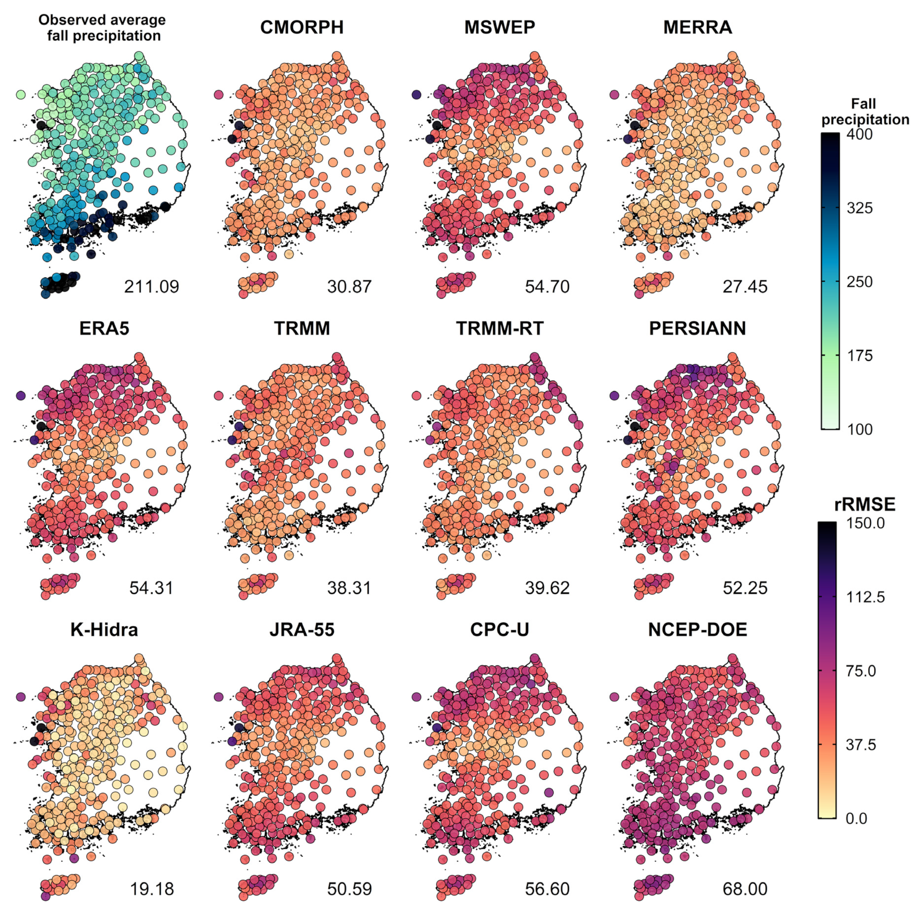
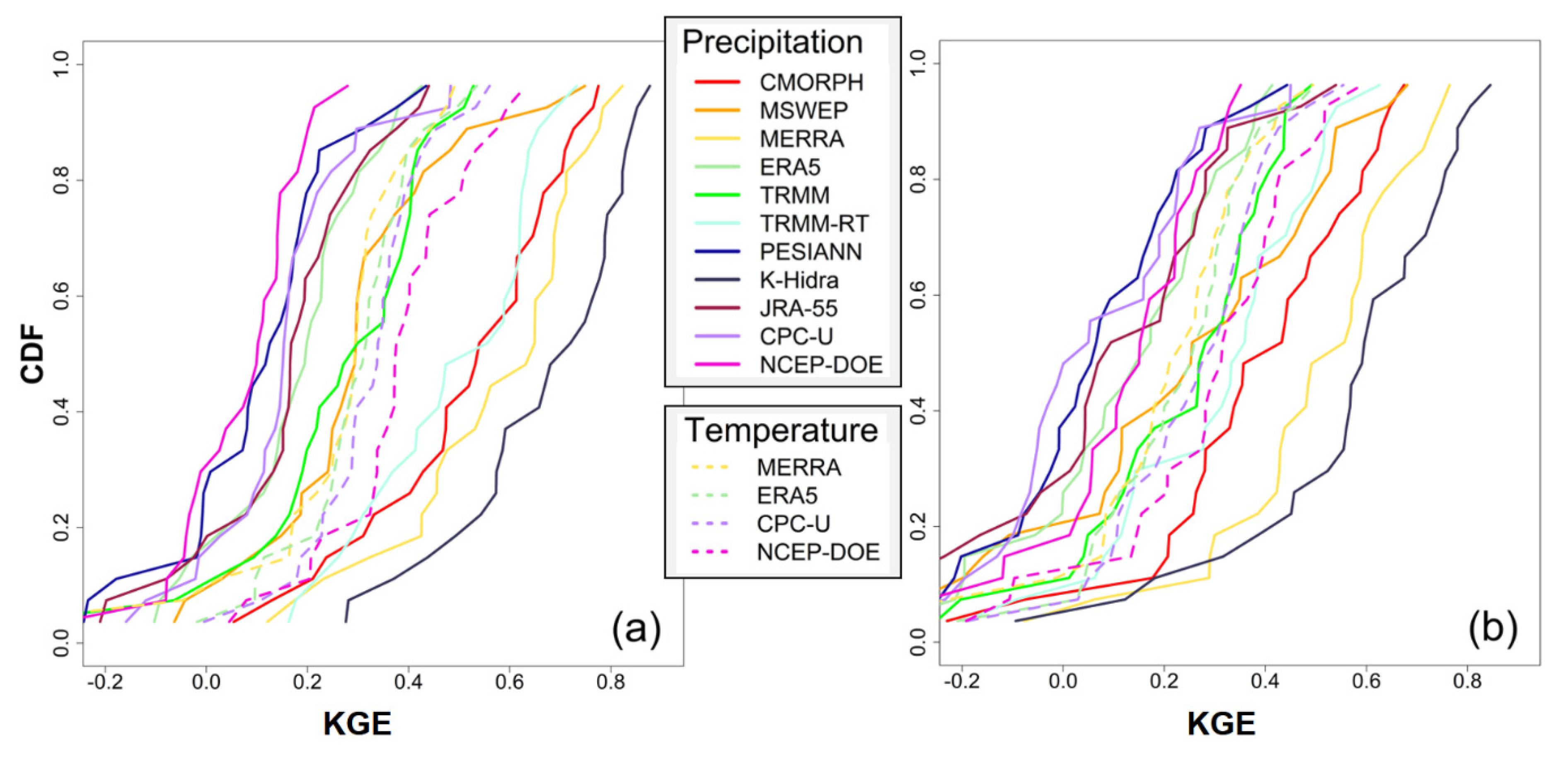
4.1. Evaluation of Gridded Climate Datasets

In this section, we first integrate the grid-based climate products into annual and seasonal scales, the obtained time series are then evaluated along with the corresponding station-based time series. Figure 2 (Figure 3) presents the annual precipitation (maximum and minimum temperatures) at the 357 observed stations (top left) and the results of rRMSE from each of the gridded precipitation (maximum and minimum temperatures) products. Similarly, Figure S1 (Figure S2) shows the results of rMB from each of the gridded precipitation (temperature) products. Here, we note that a positive value for the rMB metric informs that the value from the grid-based products is larger than the station-based observed value on average, vice versa.
Model performance vary for the annual scale. Annual precipitations of the four grid-based products are less than the observations, with TRMM-RT being the least (see Figure S1). The underestimations are apparent in the southern coastal region, including Jeju Island, the largest island of South Korea. On the other hand, seven grid-based datasets produce greater precipitation than the observations, with PERSIANN being the greatest. However, despite the general performance of each model, the majority of them exhibited considerable overestimations in the northwestern region. Based on the rRMSE metric, K-Hidra and MERRA produce the lowest rRMSE values (13.41 and 15.06), particularly with the smallest biases over the central region of our study area, whereas PERSIANN, MSWEP and NCEP-DOE yield the largest rRMSE values (27.02, 25.55, and 52.91). The spatial patterns of the maximum and minimum temperatures vary substantially de-pending on the dataset and variable of interest. For instance, maximum temperatures of ERA5 produce severe bias in the southern area whereas ERA5 offers the most reliable maximum temperatures in the northern region. Similarly, NCEP-DOE offers the most re-liable maximum temperatures while it yields substantial bias for minimum temperatures over the northern region. Overall, CPC-U performs the best for both maximum and mini-mum temperatures followed by the ERA5 dataset although the ERA5 dataset produces less maximum temperature and greater minimum temperature (see Figure S2).
To further investigate grid-based climate products on the seasonal scale, Figure 4 and Figure 5 show spatial patterns of seasonal precipitation rRMSE for spring (MAM) and fall (SON). Also, spatial patterns of seasonal precipitation metrics for other seasons and those for temperatures are presented in the supporting information (see Figures S3–S8). Overall, results for seasonal analyses are similar to those obtained for the annual scale. K-Hidra and MERRA show the best performance in seasonal precipitation with less bias for all seasons compared to the other products. Interestingly, less relative biases for precipitation are often found in spring when compared to fall. For example, the median E r R M S E for K-Hidra is 16.93 and 19.18 while TRMM is 29.06 and 38.31 for the spring and fall seasons, respectively. However, the relatively large biases for fall may not indicate that the datasets exhibited substantial under- or over-estimations for the seasonal scales except for the NCEP-DOE dataset (see Figure S7). For both minimum and maximum temperatures, CPC-U and ERA5 show the best performance. Different from its reliable performance concerning precipitation, MERRA yields considerable biases across all seasons with the biases being the most severe in winter. The results suggest that the combinations of the MERRA precipitation dataset with the different temperature products may provide more reliable hydrologic simulations in representing spatial- and temporal variability over the study area, which is addressed in the following section.

4.2. Evaluation of Hydrological Modeling

In this section, the performances in the hydrological model simulations are illustrated by using the results of all 44 combinations of precipitation and temperature datasets. Figure 6 shows the mean results of E K G E and E N S E for daily streamflow simulations over the calibration and validation periods. Moreover, the details of each separated result are provided in the supporting information (see Figures S9 and S10).
In Figure 6, similar performance patterns are obtained in both results of E K G E and E N S E of daily streamflow simulations. This suggests that using a single metric to analyze the patterns may be acceptable and thus E K G E is retained for describing the remaining results. Several insights emerge from the figure. First, there is considerable variation in performance across datasets. For example, the combination of MERRA precipitation and ERA5 temperatures leads to substantially reliable performance for E K G E with 0.52 while the combination of CPC-U precipitation and MERRA temperatures yields a relatively poor E K G E with −0.02 in the validation period. It informs that the choice of forcing datasets is indeed quite relevant in hydrological modeling. Second, the choice of precipitation dataset plays a crucial role whereas the choice of temperatures provides less impact on hydrological performance. In particular, all four-temperature datasets yield similar performance although MERRA is consistently the worst of the four. Third, the combination of K-Hidra precipitation and CPC-U temperatures outperforms all other combinations. It is followed by the combination of K-Hidra precipitation and ERA5 temperatures. Also, the MERRA precipitation-based simulations perform well. Their superiorities are also observed when the evaluations are focused on low and high flows (see Figure S11). Summing up, these results support that higher reliability in the climate products leads to more accurate hydrological performance since K-Hidra and MERRA show the best performance in representing spatial and temporal behavior of precipitation over the study area (see Section 4.1).
Presented in Figure 7 are the results of E K G E of all 26 gauges for the precipitation-focused aggregation (i.e., average of E K G E for four temperature-based simulations with a specific precipitation dataset) and temperature-focused aggregation (i.e., average of E K G E for eleven precipitation-based simulations with a specific temperature dataset) over the calibration and validation periods, respectively. Again, the results confirm those found in Figure 6, particularly for the first and second insights. There are considerable variations in eleven precipitation-focused aggregations while less variations are observed in four temperature-focused aggregation. Both indicate the choice of precipitation dataset is more important that the temperature choice. Moreover, the results underline the outperformance of K-Hidra and MERRA in contrast to the relatively poor performance of the PERSIANN and CPC-U precipitation datasets, which is also found in Figure 6.

4.3. Evaluation of Hydrological Performance by Combining Multiple Datasets

The spatial distribution of E K G E for the simulations from forcing datasets in different combinations is presented in Figure 8. Here, six ensemble-based simulations are considered, including the average of all ensemble input (i.e., utilizing the mean of the eleven precipitation and four temperature datasets), the average of reliable ensemble input (i.e., utilizing the mean of the four best precipitation [K-Hidra, MERRA, TRMM, and CMORPH] and two best temperature datasets [ERA5 and CPC-U]), the average of highly reliable ensemble input (i.e., utilizing the mean of two best precipitation [K-Hidra and MERRA] and the CPC-U temperature datasets), the average of all ensemble output with forty-four combinations of climate forcing, the average of reliable ensemble output from the eight combinations (i.e., = four precipitation × two temperatures), and the average of highly reliable ensemble output from the two combinations (i.e., = two precipitation × one temperatures) of climate forcing. The ensemble simulations are independently calibrated and their accuracies are then evaluated over the validation period (see Figure 8). We also present the spatial distribution of E K G E obtained by the hydrologic simulation with the combination of K-Hidra precipitation and CPC-U temperatures in the top-left as a baseline single-based simulation. All the other maps illustrate the difference in KGE values between each ensemble-based simulation and baseline simulation. A red color informs a better performance for the ensemble-based simulations; blue, a worse performance.
The average of all ensemble input generally shows improved model performance (the mean of E K G E = 0.47) when compared to that of all ensemble output (the mean of E K G E   = 0.42), informing that utilizing multiple input may generate more stable climate estimates, and leads to a better streamflow simulation. However, a single-based simulation with the best performing dataset shows higher accuracy (the mean of E K G E = 0.60), which is contrary to the previous work showing that ensemble-based simulations improve model performance [49].
Perhaps, our results are at odds with those of previous studies due to the substantial bias in some datasets. To further investigate the hypothesis that a single-based simulation would outperform an ensemble-based simulation, the number of datasets used for ensemble simulations are decreased to bolster the performance in the ensemble-based results by using only a part of the datasets (i.e., the average of marginally and highly reliable ensemble simulations). The reliable ensemble-based simulations for input and output produced 0.47 and 0.48 as the mean of E K G E , indicating they are less accurate than a single-based simulation. Although highly reliable ensemble-based simulations for input (the mean of E K G E = 0.61) and output (the mean of E K G E = 0.59) show higher performance than other ensemble-based simulations, their accuracies differ a little from that of a single-based simulation. Although there is a small improvement in performance by taking the mean of the ensemble results, the required additional increased computational burden makes this strategy much less appealing, informing that ensemble-based simulations may not be effective for hydrological modeling over our study area.

5. Conclusions

The performance of hydrological modeling is fundamentally rooted in the quality of climate forcing data. While station-based observations have traditionally been employed in a number of applications, they are often limited in both temporal and spatial scales. To be specific, station-based observations suffer from some obstacles such as missing data, measured errors and changes in geographical locations of weather stations including their displacement. To mitigate these limitations, gridded climate datasets have recently received increasing attention. This study contributes to evaluating a number of climate datasets (i.e., eleven precipitation datasets and four temperature datasets) by combining gridded rainfall and temperature datasets to identify which climate gridded datasets would be most suitable for use in streamflow estimation over the study area.
Our results indicate that significant differences exist among the gridded datasets. For example, K-Hidra produced the lowest rRMSE value (13.41) for the annual scale in comparison with the corresponding station-based time series, whereas PERSIANN and NCEP-DOE yielded large rRMSE values (27.02 and 52.91). The results confirm that some datasets represent the variability of local climate better than others. The differences are further verified when the datasets are employed in a hydrological model. The differences may be related to the spatial resolution of the original satellite products. For example, K-Hidra has relatively fine spatial resolution whereas NCEP-DOE is developed with coarse spatial resolution. In addition, the importance of dataset selection varies depending on the variable. While precipitation datasets are the primary drivers of reliability for simulations, less variation from the four temperature datasets (MERRA, ERA5, CPC-U, and NCEP-DOE) is observed. This could likely be attributed to the relatively small spatial and temporal variability in temperature, at least when compared to those for precipitation. Significant differences in the performance of the hydrological model also encourage the exploration of different climate datasets to choose the most suitable one before the regional-scale hydrological modeling.
Among all the datasets evaluated in this study, K-Hidra and CPC-U represent the best datasets for precipitation and temperature, respectively, over the study area. There are possible reasons for the superior performance of both K-Hidra and CPC-U in representing the regional variability of precipitation and temperature. These datasets are based on reanalysis-based estimations, which are known to be more reliable than the satellite-based products [82,83]. In particular, K-Hidra is the closest relative (in terms of data construction) to the chosen reference stations over South Korea. Other studies have mentioned its high quality for our study area [84,85]. Also, from the results, we find that a reliable precipitation product is not necessarily the best for representing temperature (e.g., MERRA). Accordingly, the hydrological simulations generated using the combination of different datasets for forcing are more reliable over the study area and may be conducive to a distributed hydrological modeling over the study area, including climate change assessment.
Previous studies have addressed that if significant differences in available datasets exist, one cogent approach is to consider combining forced datasets or combining simulated outputs using an ensemble approach. This study explores the possible superiority of an ensemble-based approach for integrating hydrological modeling over the wide study area. We find that combining forcing datasets or combining simulated streamflow may prove less effective when compared to a single-based simulation with the best per-forming dataset. However, the results may be limited since this study just explores a simple averaging approach for generating an ensemble simulation while a number of diverse techniques (e.g., the Bayesian model averaging [86]) have been introduced in the field of hydro-climatology. However, such exploration is beyond the scope of this work.
In spite of efforts to implement a comprehensive assessment of the meteorological datasets, the results obtained may be subject to some uncertainties and limitations. First, the original gridded datasets are composed of different spatial and temporal resolutions. For example, the spatial and temporal resolutions of MSWEP are 0.10° and a three-hourly basis, respectively, whereas CPC-U has 0.50° and a daily basis as its spatial and temporal resolutions. As denoted in [87], analysis from sub-daily modeling would be favorable particularly for small basins although some of the datasets (e.g., PERSIANN) utilized were limited to a daily time step. Our interpolation processes for comparison purposes might induce additional uncertainties for climate datasets. Second, our evaluations for climate datasets are relatively straightforward. To further obtain the insightful differences among the datasets, additional categorical-based statistics may be required, similar to the analysis in [88]. Third, the hydrological performance of the grid dataset is related to deficiencies or structures in hydrological modeling. From this aspect, the final parameter set of our hydrologic model could be limited by the possibility of obtaining equally reliable model performance from different parameter sets (i.e., equifinality) [89]. Moreover, a multisite pooled calibration strategy is adopted for our hydrologic modeling by maximizing the KGE metric. We initially considered a multiscale parameter regionalization (MPR) scheme [90] to represent seamless spatial patterns of hydrological processes but did not utilize it since the performance remarkably decreased (not shown). The multiple calibration scheme-based approaches deserve investigation in future research. Accordingly, the representation of other metrics (e.g., NSE, peak flow reproduction and variance of streamflow) and their combined metrics along with utilization of other distributed hydrological models, merit consideration in analyzing the hydrological performance of grid datasets.
The findings of this study provide a vital insight into the utility of meteorological datasets for regional hydrological applications. Overall, our results emphasize the importance of selecting suitable climate datasets in regional hydrological modeling. As future research, we will further seek to determine suitable data uncertainty bounds when provided with multiple datasets for hydrological modelling based on the approach in [50]. Regarding this research initiative, combining multiple datasets for model calibration will also be feasible to pursue a robust modeling parametrization.

Supplementary Materials

The following supporting information can be downloaded at: https://www.mdpi.com/article/10.3390/rs14153535/s1, Figure S1: Spatial patterns of rMB for annual precipitation of the grid datasets from observations. The median values of rMB metric at 356 stations are also presented for each sub-figure; Figure S2: Spatial patterns of rMB for annual maximum (top) and minimum (bottom) temperatures of four grid datasets (each column) from observations. The median value of rMB metric at 356 stations is also presented for each sub-figure; Figure S3: Spatial patterns of rRMSE for summer (JJA) precipitation of the grid datasets from observations. The median values of rRMSE metric across 356 stations are also presented for each sub-figure; Figure S4: As in Figure 4 but for winter (DJF) precipitation; Figure S5: Spatial patterns of MB for spring precipitation of the grid datasets from observations. The median values of MB metric at 356 stations are also presented for each sub-figure; Figure S6: Spatial patterns of MB for summer precipitation of the grid datasets from observations. The median values of MB metric at 356 stations are also presented for each sub-figure; Figure S7: Spatial patterns of MB for fall precipitation of the grid datasets from observations. The median values of MB metric at 356 stations are also presented for each sub-figure; Figure S8: Spatial patterns of MB for winter precipitation of the grid datasets from observations. The median values of MB metric at 356 stations are also presented for each sub-figure; Figure S9: Kling-Gupta efficiency of daily streamflow over the calibration period (2008–2013) for forty-four combinations of eleven precipitation datasets (y-axis) and four temperature datasets (subplots on x-axis) used as forcing in the VIC model. Each boxplot has 26 values for each streamflow gauging station; Figure S10: Kling-Gupta efficiency of daily streamflow over the calibration period (2014–2019) for forty-four combinations of eleven precipitation datasets (y-axis) and four temperature datasets (subplots on x-axis) used as forcing in the VIC model. Each boxplot has 26 values for each streamflow gauging station; Figure S11: Average of the logged transformed (E_logNSE) and modified (E_absNSE) Nash-Sutcliffe efficiencies for the 26 daily streamflow simulations during (left) the calibration period and (right) the validation period for forty-four combinations of 11 precipitation datasets (y-axis) and 4 temperature datasets (x-axis) employed as forcing in hydrological modeling.

Author Contributions

Conceptualization, K.-H.A.; methodology, D.-G.L.; software, D.-G.L.; validation, D.-G.L.; formal analysis, D.-G.L.; investigation, D.-G.L.; resources, D.-G.L.; data curation, D.-G.L.; writing—original draft preparation, review and editing, K.-H.A.; visualization, D.-G.L.; supervision, K.-H.A.; project administration, K.-H.A.; funding acquisition, K.-H.A. All authors have read and agreed to the published version of the manuscript.

Funding

This work was supported by the National Research Foundation of Korea (NRF) grant funded by the Korea government (MSIT) (No. 2019R1C1C1002438). Also, this work was partially supported by the research grant from the Kongju National University in 2022.

Data Availability Statement

Not applicable.

Conflicts of Interest

The authors declare no conflict of interest.

References

  1. Dembélé, M.; Schaefli, B.; Van De Giesen, N.; Mariéthoz, G. Suitability of 17 Gridded Rainfall and Temperature Datasets for Large-Scale Hydrological Modelling in West Africa. Hydrol. Earth Syst. Sci. 2020, 24, 5379–5406. [Google Scholar] [CrossRef]
  2. Zandler, H.; Haag, I.; Samimi, C. Evaluation Needs and Temporal Performance Differences of Gridded Precipitation Products in Peripheral Mountain Regions. Sci. Rep. 2019, 9, 15118. [Google Scholar] [CrossRef] [Green Version]
  3. Hou, A.Y.; Kakar, R.K.; Neeck, S.; Azarbarzin, A.A.; Kummerow, C.D.; Kojima, M.; Oki, R.; Nakamura, K.; Iguchi, T. The Global Precipitation Measurement Mission. Bull. Am. Meteorol. Soc. 2014, 95, 701–722. [Google Scholar] [CrossRef]
  4. Urita, S.; Saito, H.; Matsuyama, H. Temporal and Spatial Discontinuity of Radar/Raingauge-Analyzed Precipitation That Appeared in Relation to the Modification of Its Spatial Resolution. Hydrol. Res. Lett. 2011, 5, 37–41. [Google Scholar] [CrossRef] [Green Version]
  5. Shen, Y.; Xiong, A. Validation and Comparison of a New Gauge-Based Precipitation Analysis over Mainland China. Int. J. Climatol. 2016, 36, 252–265. [Google Scholar] [CrossRef]
  6. Sarachi, S.; Hsu, K.; Sorooshian, S. A Statistical Model for the Uncertainty Analysis of Satellite Precipitation Products. J. Hydrometeorol. 2015, 16, 2101–2117. [Google Scholar] [CrossRef]
  7. Sun, Q.; Miao, C.; Duan, Q.; Ashouri, H.; Sorooshian, S.; Hsu, K.-L. A Review of Global Precipitation Data Sets: Data Sources, Estimation, and Intercomparisons. Rev. Geophys. 2018, 56, 79–107. [Google Scholar] [CrossRef] [Green Version]
  8. Bosilovich, M.G.; Chen, J.; Robertson, F.R.; Adler, R.F. Evaluation of Global Precipitation in Reanalyses. J. Appl. Meteorol. Climatol. 2008, 47, 2279–2299. [Google Scholar] [CrossRef]
  9. Zhang, L.; Chen, X.; Lai, R.; Zhu, Z. Performance of Satellite-Based and Reanalysis Precipitation Products under Multi-Temporal Scales and Extreme Weather in Mainland China. J. Hydrol. 2021, 605, 127389. [Google Scholar] [CrossRef]
  10. Huffman, G.J.; Bolvin, D.T.; Nelkin, E.J.; Wolff, D.B.; Adler, R.F.; Gu, G.; Hong, Y.; Bowman, K.P.; Stocker, E.F. The TRMM Multisatellite Precipitation Analysis (TMPA): Quasi-Global, Multiyear, Combined-Sensor Precipitation Estimates at Fine Scales. J. Hydrometeorol. 2007, 8, 38–55. [Google Scholar] [CrossRef]
  11. Kidd, C.; Huffman, G. Global Precipitation Measurement. Meteorol. Appl. 2011, 18, 334–353. [Google Scholar] [CrossRef]
  12. Prakash, S.; Mitra, A.K.; AghaKouchak, A.; Liu, Z.; Norouzi, H.; Pai, D. A Preliminary Assessment of GPM-Based Multi-Satellite Precipitation Estimates over a Monsoon Dominated Region. J. Hydrol. 2018, 556, 865–876. [Google Scholar] [CrossRef] [Green Version]
  13. Sorooshian, S.; Hsu, K.-L.; Gao, X.; Gupta, H.V.; Imam, B.; Braithwaite, D. Evaluation of PERSIANN System Satellite-Based Estimates of Tropical Rainfall. Bull. Am. Meteorol. Soc. 2000, 81, 2035–2046. [Google Scholar] [CrossRef] [Green Version]
  14. Joyce, R.J.; Janowiak, J.E.; Arkin, P.A.; Xie, P. CMORPH: A Method That Produces Global Precipitation Estimates from Passive Microwave and Infrared Data at High Spatial and Temporal Resolution. J. Hydrometeorol. 2004, 5, 487–503. [Google Scholar] [CrossRef]
  15. Turk, F.J.; Mostovoy, G.V.; Anantharaj, V.G. Soil Moisture Sensitivity to NRL-Blend High-Resolution Precipitation Products: Analysis of Simulations with Two Land Surface Models. IEEE J. Sel. Top. Appl. Earth Obs. Remote Sens. 2009, 3, 32–48. [Google Scholar] [CrossRef]
  16. Alazzy, A.A.; Lü, H.; Chen, R.; Ali, A.B.; Zhu, Y.; Su, J. Evaluation of Satellite Precipitation Products and Their Potential Influence on Hydrological Modeling over the Ganzi River Basin of the Tibetan Plateau. Adv. Meteorol. 2017, 2017, 3695285. [Google Scholar] [CrossRef] [Green Version]
  17. Berg, P.; Donnelly, C.; Gustafsson, D. Near-Real-Time Adjusted Reanalysis Forcing Data for Hydrology. Hydrol. Earth Syst. Sci. 2018, 22, 989–1000. [Google Scholar] [CrossRef] [Green Version]
  18. Lee, D.-G.; Ahn, K.-H. A Stacking Ensemble Model for Hydrological Post-Processing to Improve Streamflow Forecasts at Medium-Range Timescales over South Korea. J. Hydrol. 2021, 600, 126681. [Google Scholar] [CrossRef]
  19. Wu, H.; Adler, R.F.; Tian, Y.; Huffman, G.J.; Li, H.; Wang, J. Real-Time Global Flood Estimation Using Satellite-Based Precipitation and a Coupled Land Surface and Routing Model. Water Resour. Res. 2014, 50, 2693–2717. [Google Scholar] [CrossRef] [Green Version]
  20. Buarque, D.C.; de Paiva, R.C.D.; Clarke, R.T.; Mendes, C.A.B. A Comparison of Amazon Rainfall Characteristics Derived from TRMM, CMORPH and the Brazilian National Rain Gauge Network. J. Geophys. Res. Atmos. 2011, 116, D19105. [Google Scholar] [CrossRef]
  21. He, Z.; Yang, L.; Tian, F.; Ni, G.; Hou, A.; Lu, H. Intercomparisons of Rainfall Estimates from TRMM and GPM Multisatellite Products over the Upper Mekong River Basin. J. Hydrometeorol. 2017, 18, 413–430. [Google Scholar] [CrossRef]
  22. Le Coz, C.; van de Giesen, N. Comparison of Rainfall Products over Sub-Saharan Africa. J. Hydrometeorol. 2020, 21, 553–596. [Google Scholar] [CrossRef]
  23. Caroletti, G.N.; Coscarelli, R.; Caloiero, T. Validation of Satellite, Reanalysis and Rcm Data of Monthly Rainfall in Calabria (Southern Italy). Remote Sens. 2019, 11, 1625. [Google Scholar] [CrossRef] [Green Version]
  24. Gupta, V.; Jain, M.K.; Singh, P.K.; Singh, V. An Assessment of Global Satellite-Based Precipitation Datasets in Capturing Precipitation Extremes: A Comparison with Observed Precipitation Dataset in India. Int. J. Climatol. 2020, 40, 3667–3688. [Google Scholar] [CrossRef]
  25. Xu, R.; Tian, F.; Yang, L.; Hu, H.; Lu, H.; Hou, A. Ground Validation of GPM IMERG and TRMM 3B42V7 Rainfall Products over Southern Tibetan Plateau Based on a High-Density Rain Gauge Network. J. Geophys. Res. Atmos. 2017, 122, 910–924. [Google Scholar] [CrossRef]
  26. Wang, W.; Lu, H. Evaluation and Comparison of Newest GPM and TRMM Products over Mekong River Basin at Daily Scale. In Proceedings of the 2016 IEEE International Geoscience and Remote Sensing Symposium (IGARSS), Beijing, China, 10–15 July 2016; IEEE: Piscataway, NJ, USA, 2016; pp. 613–616. [Google Scholar]
  27. Nanding, N.; Wu, H.; Tao, J.; Maggioni, V.; Beck, H.E.; Zhou, N.; Huang, M.; Huang, Z. Assessment of Precipitation Error Propagation in Discharge Simulations over the Contiguous United States. J. Hydrometeorol. 2021, 22, 1987–2008. [Google Scholar] [CrossRef]
  28. Nkiaka, E.; Nawaz, N.; Lovett, J.C. Evaluating Global Reanalysis Datasets as Input for Hydrological Modelling in the Sudano-Sahel Region. Hydrology 2017, 4, 13. [Google Scholar] [CrossRef] [Green Version]
  29. He, Z.; Hu, H.; Tian, F.; Ni, G.; Hu, Q. Correcting the TRMM Rainfall Product for Hydrological Modelling in Sparsely-Gauged Mountainous Basins. Hydrol. Sci. J. 2017, 62, 306–318. [Google Scholar] [CrossRef]
  30. Camici, S.; Ciabatta, L.; Massari, C.; Brocca, L. How Reliable Are Satellite Precipitation Estimates for Driving Hydrological Models: A Verification Study over the Mediterranean Area. J. Hydrol. 2018, 563, 950–961. [Google Scholar] [CrossRef]
  31. Poméon, T.; Jackisch, D.; Diekkrüger, B. Evaluating the Performance of Remotely Sensed and Reanalysed Precipitation Data over West Africa Using HBV Light. J. Hydrol. 2017, 547, 222–235. [Google Scholar] [CrossRef]
  32. Wang, N.; Liu, W.; Sun, F.; Yao, Z.; Wang, H.; Liu, W. Evaluating Satellite-Based and Reanalysis Precipitation Datasets with Gauge-Observed Data and Hydrological Modeling in the Xihe River Basin, China. Atmos. Res. 2020, 234, 104746. [Google Scholar] [CrossRef]
  33. Hrachowitz, M.; Clark, M.P. HESS Opinions: The Complementary Merits of Competing Modelling Philosophies in Hydrology. Hydrol. Earth Syst. Sci. 2017, 21, 3953–3973. [Google Scholar] [CrossRef] [Green Version]
  34. Zambrano-Bigiarini, M.; Nauditt, A.; Birkel, C.; Verbist, K.; Ribbe, L. Temporal and Spatial Evaluation of Satellite-Based Rainfall Estimates across the Complex Topographical and Climatic Gradients of Chile. Hydrol. Earth Syst. Sci. 2017, 21, 1295–1320. [Google Scholar] [CrossRef] [Green Version]
  35. Maggioni, V.; Massari, C. On the Performance of Satellite Precipitation Products in Riverine Flood Modeling: A Review. J. Hydrol. 2018, 558, 214–224. [Google Scholar] [CrossRef]
  36. Laiti, L.; Mallucci, S.; Piccolroaz, S.; Bellin, A.; Zardi, D.; Fiori, A.; Nikulin, G.; Majone, B. Testing the Hydrological Coherence of High-Resolution Gridded Precipitation and Temperature Data Sets. Water Resour. Res. 2018, 54, 1999–2016. [Google Scholar] [CrossRef] [Green Version]
  37. Bhattacharya, T.; Khare, D.; Arora, M. A Case Study for the Assessment of the Suitability of Gridded Reanalysis Weather Data for Hydrological Simulation in Beas River Basin of North Western Himalaya. Appl. Water Sci. 2019, 9, 110. [Google Scholar] [CrossRef] [Green Version]
  38. Blacutt, L.A.; Herdies, D.L.; de Gonçalves, L.G.G.; Vila, D.A.; Andrade, M. Precipitation Comparison for the CFSR, MERRA, TRMM3B42 and Combined Scheme Datasets in Bolivia. Atmos. Res. 2015, 163, 117–131. [Google Scholar] [CrossRef] [Green Version]
  39. Jiang, Q.; Li, W.; Fan, Z.; He, X.; Sun, W.; Chen, S.; Wen, J.; Gao, J.; Wang, J. Evaluation of the ERA5 Reanalysis Precipitation Dataset over Chinese Mainland. J. Hydrol. 2021, 595, 125660. [Google Scholar] [CrossRef]
  40. Tarek, M.; Brissette, F.P.; Arsenault, R. Evaluation of the ERA5 Reanalysis as a Potential Reference Dataset for Hydrological Modelling over North America. Hydrol. Earth Syst. Sci. 2020, 24, 2527–2544. [Google Scholar] [CrossRef]
  41. Kim, J.P.; Jung, I.W.; Park, K.W.; Yoon, S.K.; Lee, D. Hydrological Utility and Uncertainty of Multi-Satellite Precipitation Products in the Mountainous Region of South Korea. Remote Sens. 2016, 8, 608. [Google Scholar] [CrossRef] [Green Version]
  42. Qi, W.; Zhang, C.; Fu, G.; Sweetapple, C.; Zhou, H. Evaluation of Global Fine-Resolution Precipitation Products and Their Uncertainty Quantification in Ensemble Discharge Simulations. Hydrol. Earth Syst. Sci. 2016, 20, 903–920. [Google Scholar] [CrossRef] [Green Version]
  43. Shawul, A.A.; Chakma, S. Suitability of Global Precipitation Estimates for Hydrologic Prediction in the Main Watersheds of Upper Awash Basin. Environ. Earth Sci. 2020, 79, 53. [Google Scholar] [CrossRef]
  44. Tang, X.; Zhang, J.; Gao, C.; Ruben, G.B.; Wang, G. Assessing the Uncertainties of Four Precipitation Products for Swat Modeling in Mekong River Basin. Remote Sens. 2019, 11, 304. [Google Scholar] [CrossRef] [Green Version]
  45. Tramblay, Y.; Thiemig, V.; Dezetter, A.; Hanich, L. Evaluation of Satellite-Based Rainfall Products for Hydrological Modelling in Morocco. Hydrol. Sci. J. 2016, 61, 2509–2519. [Google Scholar] [CrossRef] [Green Version]
  46. Stisen, S.; Højberg, A.; Troldborg, L.; Refsgaard, J.; Christensen, B.; Olsen, M.; Henriksen, H. On the Importance of Appropriate Precipitation Gauge Catch Correction for Hydrological Modelling at Mid to High Latitudes. Hydrol. Earth Syst. Sci. 2012, 16, 4157–4176. [Google Scholar] [CrossRef] [Green Version]
  47. Cornes, R.C.; van der Schrier, G.; van den Besselaar, E.J.; Jones, P.D. An Ensemble Version of the E-OBS Temperature and Precipitation Data Sets. J. Geophys. Res. Atmos. 2018, 123, 9391–9409. [Google Scholar] [CrossRef] [Green Version]
  48. Schreiner-McGraw, A.P.; Ajami, H. Impact of Uncertainty in Precipitation Forcing Data Sets on the Hydrologic Budget of an Integrated Hydrologic Model in Mountainous Terrain. Water Resour. Res. 2020, 56, e2020WR027639. [Google Scholar] [CrossRef]
  49. Zhu, Q.; Gao, X.; Xu, Y.-P.; Tian, Y. Merging Multi-Source Precipitation Products or Merging Their Simulated Hydrological Flows to Improve Streamflow Simulation. Hydrol. Sci. J. 2019, 64, 910–920. [Google Scholar] [CrossRef]
  50. Ahn, K.-H.; Kim, Y.-O. Incorporating Climate Model Similarities and Hydrologic Error Models to Quantify Climate Change Impacts on Future Riverine Flood Risk. J. Hydrol. 2019, 570, 118–131. [Google Scholar] [CrossRef]
  51. Alcantara, A.L.; Ahn, K.-H. Probability Distribution and Characterization of Daily Precipitation Related to Tropical Cyclones over the Korean Peninsula. Water 2020, 12, 1214. [Google Scholar] [CrossRef]
  52. Tsai, C.-L.; Kim, K.; Liou, Y.-C.; Lee, G.; Yu, C.-K. Impacts of Topography on Airflow and Precipitation in the Pyeongchang Area Seen from Multiple-Doppler Radar Observations. Mon. Weather Rev. 2018, 146, 3401–3424. [Google Scholar] [CrossRef]
  53. Xie, P.; Joyce, R.; Wu, S.; Yoo, S.-H.; Yarosh, Y.; Sun, F.; Lin, R. Reprocessed, Bias-Corrected CMORPH Global High-Resolution Precipitation Estimates from 1998. J. Hydrometeorol. 2017, 18, 1617–1641. [Google Scholar] [CrossRef]
  54. Beck, H.E.; Van Dijk, A.I.; Levizzani, V.; Schellekens, J.; Miralles, D.G.; Martens, B.; Roo, A. de MSWEP: 3-Hourly 0.25 Global Gridded Precipitation (1979–2015) by Merging Gauge, Satellite, and Reanalysis Data. Hydrol. Earth Syst. Sci. 2017, 21, 589–615. [Google Scholar] [CrossRef] [Green Version]
  55. Gelaro, R.; McCarty, W.; Suárez, M.J.; Todling, R.; Molod, A.; Takacs, L.; Randles, C.A.; Darmenov, A.; Bosilovich, M.G.; Reichle, R.; et al. The Modern-Era Retrospective Analysis for Research and Applications, Version 2 (MERRA-2). J. Clim. 2017, 30, 5419–5454. [Google Scholar] [CrossRef] [PubMed]
  56. Hersbach, H.; Bell, B.; Berrisford, P.; Hirahara, S.; Horányi, A.; Muñoz-Sabater, J.; Nicolas, J.; Peubey, C.; Radu, R.; Schepers, D.; et al. The ERA5 Global Reanalysis. Q. J. R. Meteorol. Soc. 2020, 146, 1999–2049. [Google Scholar] [CrossRef]
  57. Ashouri, H.; Hsu, K.-L.; Sorooshian, S.; Braithwaite, D.K.; Knapp, K.R.; Cecil, L.D.; Nelson, B.R.; Prat, O.P. PERSIANN-CDR: Daily Precipitation Climate Data Record from Multisatellite Observations for Hydrological and Climate Studies. Bull. Am. Meteorol. Soc. 2015, 96, 69–83. [Google Scholar] [CrossRef] [Green Version]
  58. Noh, G.-H.; Ahn, K.-H. New Gridded Rainfall Dataset over the Korean Peninsula: Gap Infilling, Reconstruction, and Validation. J. Int. Climatol. 2021, 42, 435–452. [Google Scholar] [CrossRef]
  59. Kobayashi, S.; Ota, Y.; Harada, Y.; Ebita, A.; Moriya, M.; Onoda, H.; Onogi, K.; Kamahori, H.; Kobayashi, C.; Endo, H.; et al. The JRA-55 Reanalysis: General Specifications and Basic Characteristics. J. Meteorol. Soc. Jpn. Ser. II 2015, 93, 5–48. [Google Scholar] [CrossRef] [Green Version]
  60. Chen, M.; Shi, W.; Xie, P.; Silva, V.B.; Kousky, V.E.; Wayne Higgins, R.; Janowiak, J.E. Assessing Objective Techniques for Gauge-Based Analyses of Global Daily Precipitation. J. Geophys. Res. Atmos. 2008, 113, D04110. [Google Scholar] [CrossRef]
  61. Kanamitsu, M.; Ebisuzaki, W.; Woollen, J.; Yang, S.-K.; Hnilo, J.; Fiorino, M.; Potter, G. Ncep–Doe Amip-Ii Reanalysis (r-2). Bull. Am. Meteorol. Soc. 2002, 83, 1631–1644. [Google Scholar] [CrossRef]
  62. Hoerl, A.E.; Kennard, R.W. Ridge Regression: Biased Estimation for Nonorthogonal Problems. Technometrics 1970, 12, 55–67. [Google Scholar] [CrossRef]
  63. Tibshirani, R. Regression Shrinkage and Selection via the Lasso. J. R. Stat. Soc. Ser. B Methodol. 1996, 58, 267–288. [Google Scholar] [CrossRef]
  64. WMO. Guide to the Global Observing System, 2010th ed.; Updated in 2017; WMO: Geneva, Switzerland, 2010; ISBN 978-92-63-10488-5. [Google Scholar]
  65. Durre, I.; Menne, M.J.; Gleason, B.E.; Houston, T.G.; Vose, R.S. Comprehensive Automated Quality Assurance of Daily Surface Observations. J. Appl. Meteorol. Climatol. 2010, 49, 1615–1633. [Google Scholar] [CrossRef] [Green Version]
  66. Pellarin, T.; Román-Cascón, C.; Baron, C.; Bindlish, R.; Brocca, L.; Camberlin, P.; Fernández-Prieto, D.; Kerr, Y.H.; Massari, C.; Panthou, G.; et al. The Precipitation Inferred from Soil Moisture (PrISM) near Real-Time Rainfall Product: Evaluation and Comparison. Remote Sens. 2020, 12, 481. [Google Scholar] [CrossRef] [Green Version]
  67. Sulla-Menashe, D.; Friedl, M.A. User Guide to Collection 6 MODIS Land Cover (MCD12Q1 and MCD12C1) Product. USGS Rest. VA USA 2018, 1, 18. [Google Scholar]
  68. Wieder, W.; Boehnert, J.; Bonan, G.; Langseth, M. Regridded Harmonized World Soil Database v1.2. ORNL DAAC 2014. [Google Scholar] [CrossRef]
  69. Chen, C.; Li, Z.; Song, Y.; Duan, Z.; Mo, K.; Wang, Z.; Chen, Q. Performance of Multiple Satellite Precipitation Estimates over a Typical Arid Mountainous Area of China: Spatiotemporal Patterns and Extremes. J. Hydrometeorol. 2020, 21, 533–550. [Google Scholar] [CrossRef]
  70. Falck, A.S.; Maggioni, V.; Tomasella, J.; Vila, D.A.; Diniz, F.L. Propagation of Satellite Precipitation Uncertainties through a Distributed Hydrologic Model: A Case Study in the Tocantins–Araguaia Basin in Brazil. J. Hydrol. 2015, 527, 943–957. [Google Scholar] [CrossRef]
  71. Kurtzman, D.; Navon, S.; Morin, E. Improving Interpolation of Daily Precipitation for Hydrologic Modelling: Spatial Patterns of Preferred Interpolators. Hydrol. Process. Int. J. 2009, 23, 3281–3291. [Google Scholar] [CrossRef]
  72. Gilewski, P. Impact of the Grid Resolution and Deterministic Interpolation of Precipitation on Rainfall-Runoff Modeling in a Sparsely Gauged Mountainous Catchment. Water 2021, 13, 230. [Google Scholar] [CrossRef]
  73. Liang, X.; Lettenmaier, D.P.; Wood, E.F.; Burges, S.J. A Simple Hydrologically Based Model of Land Surface Water and Energy Fluxes for General Circulation Models. J. Geophys. Res. Atmos. 1994, 99, 14415–14428. [Google Scholar] [CrossRef]
  74. Shuttleworth, W.J. Evaporation Models in Hydrology. In Land Surface Evaporation; Springer: Berlin/Heidelberg, Germany, 1991; pp. 93–120. [Google Scholar]
  75. Zhenghui, X.; Fengge, S.; Xu, L.; Qingcun, Z.; Zhenchun, H.; Yufu, G. Applications of a Surface Runoff Model with Horton and Dunne Runoff for VIC. Adv. Atmos. Sci. 2003, 20, 165–172. [Google Scholar] [CrossRef]
  76. Lohmann, D.; Raschke, E.; Nijssen, B.; Lettenmaier, D. Regional Scale Hydrology: I. Formulation of the VIC-2L Model Coupled to a Routing Model. Hydrol. Sci. J. 1998, 43, 131–141. [Google Scholar] [CrossRef]
  77. Gao, H.; Tang, Q.; Shi, X.; Zhu, C.; Bohn, T.; Su, F.; Pan, M.; Sheffield, J.; Lettenmaier, D.; Wood, E. Water Budget Record from Variable Infiltration Capacity (VIC) Model. In Algorithm Theoretical Basis Document, version 1.2; Department of Civil and Environmental Engineering, University of Washington: Seattle, WA, USA, 2009. [Google Scholar]
  78. Gupta, H.V.; Kling, H.; Yilmaz, K.K.; Martinez, G.F. Decomposition of the Mean Squared Error and NSE Performance Criteria: Implications for Improving Hydrological Modelling. J. Hydrol. 2009, 377, 80–91. [Google Scholar] [CrossRef] [Green Version]
  79. Tolson, B.A.; Shoemaker, C.A. Dynamically Dimensioned Search Algorithm for Computationally Efficient Watershed Model Calibration. Water Resour. Res. 2007, 43, 1–16. [Google Scholar] [CrossRef]
  80. Ahn, K.-H.; Palmer, R.; Steinschneider, S. A Hierarchical Bayesian Model for Regionalized Seasonal Forecasts: Application to Low Flows in the Northeastern United States. Water Resour. Res. 2017, 53, 503–521. [Google Scholar] [CrossRef]
  81. Krause, P.; Boyle, D.; Bäse, F. Comparison of Different Efficiency Criteria for Hydrological Model Assessment. Adv. Geosci. 2005, 5, 89–97. [Google Scholar] [CrossRef] [Green Version]
  82. Massari, C.; Camici, S.; Ciabatta, L.; Brocca, L. Exploiting Satellite-Based Surface Soil Moisture for Flood Forecasting in the Mediterranean Area: State Update versus Rainfall Correction. Remote Sens. 2018, 10, 292. [Google Scholar] [CrossRef] [Green Version]
  83. Tarek, M.; Brissette, F.P.; Arsenault, R. Large-Scale Analysis of Global Gridded Precipitation and Temperature Datasets for Climate Change Impact Studies. J. Hydrometeorol. 2020, 21, 2623–2640. [Google Scholar] [CrossRef]
  84. Noh, G.-H.; Ahn, K.-H. Long-Lead Predictions of Early Winter Precipitation over South Korea Using a SST Anomaly Pattern in the North Atlantic Ocean. Clim. Dyn. 2022, 58, 3455–3469. [Google Scholar] [CrossRef]
  85. Qiu, L.; Im, E.-S. Added Value of High-Resolution Climate Projections over South Korea on the Scaling of Precipitation with Temperature. Environ. Res. Lett. 2021, 16, 124034. [Google Scholar] [CrossRef]
  86. Ahn, K.-H.; Merwade, V. The Effect of Land Cover Change on Duration and Severity of High and Low Flows. Hydrol. Process. 2017, 31, 133–149. [Google Scholar] [CrossRef]
  87. Bevelhimer, M.S.; McManamay, R.A.; O’connor, B. Characterizing Sub-Daily Flow Regimes: Implications of Hydrologic Resolution on Ecohydrology Studies. River Res. Appl. 2015, 31, 867–879. [Google Scholar] [CrossRef]
  88. Haile, A.T.; Rientjes, T.; Gieske, A.; Gebremichael, M. Multispectral Remote Sensing for Rainfall Detection and Estimation at the Source of the Blue Nile River. Int. J. Appl. Earth Obs. Geoinf. 2010, 12, S76–S82. [Google Scholar] [CrossRef]
  89. Silvestro, F.; Gabellani, S.; Rudari, R.; Delogu, F.; Laiolo, P.; Boni, G. Uncertainty Reduction and Parameter Estimation of a Distributed Hydrological Model with Ground and Remote-Sensing Data. Hydrol. Earth Syst. Sci. 2015, 19, 1727–1751. [Google Scholar] [CrossRef] [Green Version]
  90. Samaniego, L.; Kumar, R.; Attinger, S. Multiscale Parameter Regionalization of a Grid-Based Hydrologic Model at the Mesoscale. Water Resour. Res. 2010, 46, W05523. [Google Scholar] [CrossRef] [Green Version]
Figure 1. Locations of the selected 356 climate stations, 26 streamflow gauges, and 0.1° × 0.1° grids for hydrological modeling used in this study alongside the maps of three datasets (topography, soil types and land covers).
Remotesensing 14 03535 g001
Figure 2. Spatial patterns of rRMSE for annual precipitation of the grid datasets from observations. The median values of rRMSE metric across 356 stations are also presented for each sub-figure.
Remotesensing 14 03535 g002
Figure 3. Spatial patterns of rRMSE for annual maximum (top) and minimum (bottom) temperatures of four grid datasets (each column) from observations. The median value of rRMSE metric at 356 stations is also presented for each sub-figure.
Remotesensing 14 03535 g003
Figure 4. Spatial patterns of rRMSE for spring (MAM) precipitation of the grid datasets from observations. The median values of rRMSE metric across 356 stations are also presented for each sub-figure.
Remotesensing 14 03535 g004
Figure 5. As in Figure 4 but for fall (SON) precipitation.
Remotesensing 14 03535 g005
Figure 6. Average of the Kling-Gupta efficiency and Nash-Sutcliffe efficiency for the 26 daily stream-flow simulations during (left) the calibration period and (right) the validation period for forty-four combinations of 11 precipitation datasets (y-axis) and 4 temperature datasets (x-axis) employed as forcing in hydrological modeling. Gray color indicates averaging value is less than zero value for each metric.
Remotesensing 14 03535 g006
Figure 7. Cumulative density functions of Kling-Gupta efficiency of all streamflow gauges for the precipitation-focused aggregation (solid line) and temperature-focused aggregation (dotted line) over (a) the calibration and (b) the validation periods.
Remotesensing 14 03535 g007
Figure 8. Spatial patterns of KGE differences between simulated streamflow from the six ensemble scenarios (described in the top of each figure) and the best-performing single simulation (top left) over the validation period.
Remotesensing 14 03535 g008
Table 1. List of meteorological grid datasets used in this study.
SymbolFull NameData SourceAdopted VariableSpatial
Resolution
Temporal
Resolution
References
CMORPHClimate Predition Center (CPC) MORPHing technique (CMORPH) bias corrected V1.0S, AP 0.25 ° Daily[53]
MSWEPMulti-Source Weighted Ensemble Precipitation (MSWEP) V2.2S, A, RP 0.10 ° 3-h[54]
MERRAModern-Era Retrospective Analysis for Research and Application 2 (rainfall: M2T1NXFLX_V5.12.4; temperature: M2SDNXSLV_ V5.12.4)S, A, RP, Tmax, Tmin 0.625 ° × 0.5 ° Hourly[55]
ERA5European Centre for Medium-range Weather Forecasts Reanalysis 5 (ERA5) hourly dataRP, Tmax, Tmin 0.25 ° Hourly[56]
TRMMTRMM Multi-satellite Precipitation Analysis (TMPA) 3B42 V7S, AP 0.25 ° 3-h[10]
TRMM-RTTRMM Multi-satellite Precipitation Analysis (TMPA) 3B42 Real Time V7SP 0.25 ° 3-h[10]
PERSIANNPrecipitation Estimation from Remotely Sensed Information using Artificial Neural Networks
(PERSIANN) Climate Data Record (CDR) V1.0
S, AP 0.25 ° Daily[57]
K-HidraKorean High-resolution Daily Rainfall (K-Hidra) V2020A, RP 0.25 ° Daily[58]
JRA-55Japanese 55-year Reanalysis (rainfall: fcst_phy2m125)RP 1.25 ° 3-h[59]
CPC-UClimate Predition Center (CPC) global unified daily dataA, RP, Tmax, Tmin 0.50 ° Daily[60]
NCEP-DOENational Centers for Environmental Prediction (NCEP)–Department of Energy (DOE) reanalysis 2 projectA, RP, Tmax, Tmin 2.50 ° 6-h[61]
Abbreviation: A: gauge; S: satellite; R: reanalysis; P: precipitation; Tmax: maximum temperature; Tmin: minimum temperature.
Table 2. Adjusted parameters of the VIC hydrological model in calibration.
No.ParameterDescriptionFeasible Range
1bVariable infiltration curve parameter0.0~0.5
2DsFraction of Dsmax where non-linear baseflow begins0.0~1.0
3DmMaximum velocity of baseflow0.0~30
4WsFraction of maximum soil moisture where non-linear baseflow occurs0.0~1.0
5S1Depth of the second layer of soil (m)0.0~1.5
6S2Depth of the third layer of soil (m)0.0~2.0
7VeloWave velocity in the linearized Saint-Venant equation (m/s)0.0~5.0
8DiffDiffusivity in the linearized Saint-Venant equation (m2/s)100~900
9NumGrid Unit Hydrograph parameter (number of linear reservoirs)0.0~20
10StoGrid Unit Hydrograph parameter (reservoir storage constant)0.0~20
Publisher’s Note: MDPI stays neutral with regard to jurisdictional claims in published maps and institutional affiliations.

