SAR Tomography Based on Atomic Norm Minimization in Urban Areas

Abstract

Synthetic aperture radar (SAR) tomography (TomoSAR) is a powerful tool for the three-dimensional (3D) reconstruction of buildings in urban areas. At present, the compressed sensing (CS) technique has been widely used in the TomoSAR inversion of urban areas because of the sparsity of the backscattering power of buildings along the elevation direction. However, this algorithm discretizes the elevation and assumes that the scatterers are located on predetermined finite grids. In fact, scatterers can lie anywhere in the elevation direction, regardless of grid point constraints. The phenomenon of scatterer positioning errors due to elevation discretization is called the off-grid effect, which will affect the height estimation accuracy of TomoSAR. To overcome this problem, we proposed a TomoSAR reconstruction algorithm based on atomic norm minimization (Tomo-ANM) in this paper. Tomo-ANM employs ANM, a continuous compressed sensing technique, to obtain scatterer positions on the continuous dictionary, thus eliminating the off-grid effect. Baseline compensation is necessary to obtain the data of virtual uniform baselines or the samples of uniform data during preprocessing. A fast realization of ANM, IVDST, is utilized to accelerate the process. Tomo-ANM was tested through simulation experiments, and the results confirmed the validity of eliminating the influence of off-grid effects and exhibited an improved location accuracy and detection rate in less time compared with the on-grid TomoSAR algorithm SL1MMER. Real data experiments based on eight staring spotlight TerraSAR-X images showed that Tomo-ANM can improve the accuracy of building height estimation by 4.83% relative to its real height.

1. Introduction

Synthetic aperture radar (SAR) is an active microwave remote sensing sensor and can provide high-resolution two-dimensional (2D) images of a scene. However, due to the oblique side-looking imaging geometry of SAR, the 2D images are actually projections of an illuminated three-dimensional (3D) scene onto a range-azimuth plane, which causes layover and foreshortening effects. This affects SAR image interpretation, especially in urban areas. Synthetic aperture radar tomography (TomoSAR) is a proven and powerful technique to solve this problem [1]. By extending the synthetic aperture principle into the elevation direction, 3D-focused images can be reconstructed using data stacks of several acquisitions from slightly different incident angles.

In general, TomoSAR inversion is a line spectral problem, where we need to recover the elevation and reflectivity of scatterers—in other words, frequencies and amplitudes of signals in an azimuth-range pixel. There are various methods for TomoSAR inversion, which can be divided into three groups. Nonparametric spectral estimation, such as beamforming [2,3] and Capon [3,4], is fast and robust but has a low resolution. Parametric spectral estimation, such as multiple signal classification (MUSIC) [3,5,6] and truncated singular value decomposition (TSVD) [7], can obtain a better resolution but needs prior information, such as the number of scatterers. Considering that there are always only a few scatterers distributed in an azimuth-range pixel in urban areas, compressed sensing (CS) theory was introduced into TomoSAR inversion [8,9]. In the case of non-uniform incomplete sampling, the CS algorithm can better solve problems such as high sidelobes to achieve super-resolution capability, and has been widely used in the SAR field, such as SAR imaging [10,11]. Compared with the spectral estimation methods, CS can maintain spatial resolution by processing pixels directly instead of a covariance matrix, thus protecting the structure of buildings from destruction. Moreover, the super resolution of the elevation dimension can be obtained through the CS technique with several and uneven baselines [12]. Therefore, the CS technique, especially $L_1$ norm minimization, is the most common method used in urban TomoSAR inversion.

The conventional TomoSAR inversion methods mentioned above are considered on-grid methods using a discretized TomoSAR model, because they assume scatterers are located exactly on predetermined finite fixed grids. Therefore, the elevation is discretized into L grids beforehand, $\mathbf{s}=[s_1,s_2,s_3,\cdots ,s_L]$, and scatterer positions are obtained on one of the L grids. However, the physical truth does not always conform to the above assumption, and scatterers in the azimuth-range pixel may lie on any position of the unambiguous elevation. Therefore, the discretized TomoSAR model will inevitably lead to location bias or detection errors owing to discretization, which is called the off-grid effect or basis mismatch [13] in CS theory. Figure 1 shows the off-grid effect in the TomoSAR elevation direction. The blue line represents a building, and we give three examples of scatterers on the building that may generate strong scattering. The elevation direction s is divided into grids. The green points are the real positions of scatterers. However, since true positions are not exactly located on the grids, the grids adjacent to true positions will be used as the result of estimated locations. Thus, there is a positioning error between the true and estimated positions of scatterers, shown by the red line in Figure 1. By increasing the number of grids and reducing the space between grids, the off-grid effect can be alleviated to some extent. However, a sampling grid that is too dense increases computation dramatically and results in a high coherence dictionary, which does not meet the incoherent property in CS theory and degrades the recovery performance [14]. For TomoSAR, the off-grid effect is also a common problem. Considering the complicated backscattering properties between the buildings and surroundings in urban areas, the estimated building heights can be inaccurate because of the discretization of elevation in the TomoSAR model.

To overcome the off-grid effect in CS theory, the first gridless sparse method was introduced [15], motivated by the concept of the atomic norm, where it is proved that the frequencies can be exactly recovered from noiseless complete data if they are appropriately separated. The atomic norm minimization (ANM) was proposed in [14] to identify unknown frequencies from incomplete data. Different from the discretized CS scheme, ANM assumes frequencies distributed in an infinite dictionary and can recover sparse signals precisely in a continuous space. Because of its good performance, the ANM algorithm has been applied to sparse SAR imaging [16], DOA [17], space–time adaptive processing (STAP) [18,19], and downward-looking sparse linear array three-dimensional SAR imaging [20].

In this paper, we propose a TomoSAR imaging algorithm based on ANM, referred to as Tomo-ANM. Two problems need to be solved to implement ANM on TomoSAR. Firstly, ANM applies to uniform acquisitions or samples from uniform acquisitions. For baselines that do not fit the above distributions, which is almost inevitable in airborne and spaceborne cases, ANM does not work well. Therefore, the uneven baselines are compensated using a sector interpolation approach [21] before TomoSAR inversion. Secondly, the solution of ANM is a non-convex problem and can be worked out as a semidefinite programming (SDP) problem, which, however, incurs high computational complexity. This becomes important for preventing the practical application of ANM to TomoSAR. The alternating direction method of multipliers (ADMM) is a first-order algorithm commonly used to accelerate SDP [22,23], which is a well-established method for large-scale problems. In this paper, we employed a fast algorithm for ANM, i.e., the iterative Vandermonde decomposition and shrinkage-thresholding (IVDST) [24] algorithm, to avoid the SDP solution and improve computational efficiency. By using ANM, Tomo-ANM can eliminate the off-grid effect completely and obtain a better location accuracy and detection rate than $L_1$ norm minimization in less time.

This paper is organized as follows. In Section 2, the tomographic SAR model and ANM basic theory are outlined, and the TomoSAR reconstruction algorithm based on ANM is proposed. In Section 3 and Section 4, simulation and real data experiments are provided to prove the effectiveness of the proposed method, respectively. We also discuss the performance of Tomo-ANM under different samples, compare two fast realizations of ANM, and discuss the parameter settings of Tomo-ANM in Section 5. Finally, conclusions are summarized in Section 6.

2. Methodology

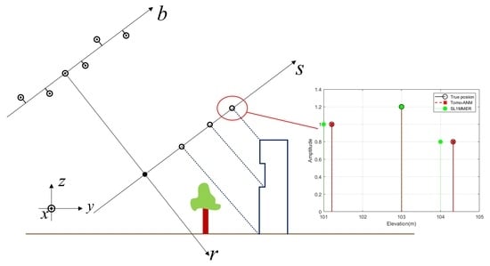
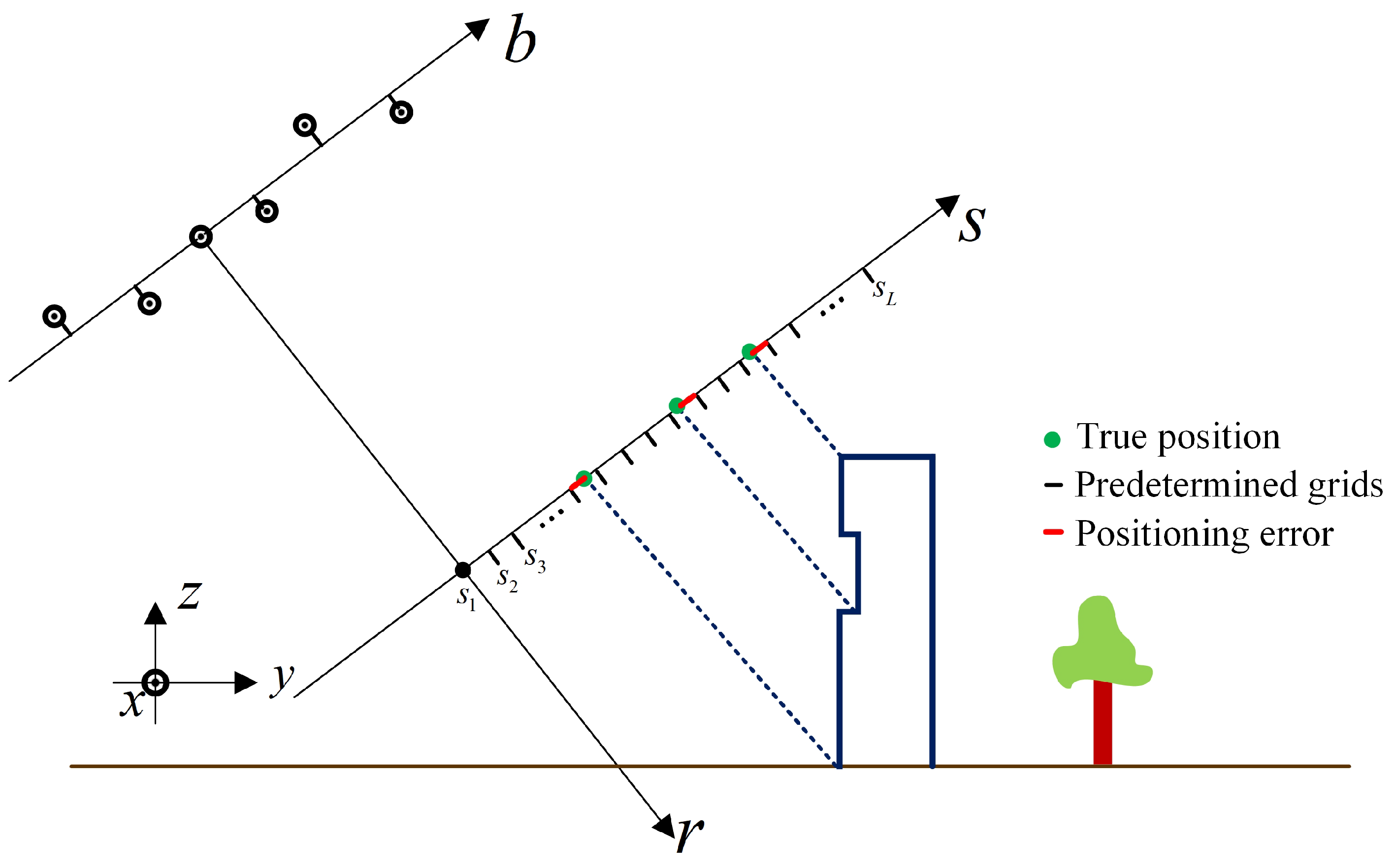
2.1. Tomographic SAR Imaging Model

In this paper, we consider N complex SAR datasets of the interested areas taken from $M(M>N)$ uniformly distributed acquisitions with slightly different incident angles. After the co-registration and phase calibration steps, the focused complex-valued measurement at the azimuth-range pixel $(x_0,r_0)$ for the nth acquisition is

$$y_n={\int }_{\mathrm{\Delta }s}\gamma \left(s\right)exp(-j2\pi {\xi }_{n}s)ds,n=1,2,\cdots ,N$$

(1)

where $\gamma \left(s\right)$ is the reflectivity along elevation s and $\mathrm{\Delta }s$ is the range of elevation. ${\xi }_n=2b_n/\lambda r_0$ is spatial frequency, where $b_n$ represents the perpendicular baseline and $\lambda$ is the wavelength.

Generally, to obtain true positions of different scatterers in the same azimuth-range pixel, the elevation s should be discretized by $s_l(l=1,2,\cdots ,L)$. TomoSAR model (1) becomes

$$y_n=\sum _{l=1}^L\gamma \left(s_l\right)exp(-j2\pi {\xi }_n{s}_l),l=1,2,\cdots ,L.$$

(2)

Inthe presence of noise $\mathbf{w}$, the TomoSAR signal model (2) can be approximated by

$$\mathbf{Y}=\mathbf{R}\mathbf{\gamma }+\mathbf{w}$$

(3)

where $\mathbf{Y}$ is the measurement vector of length N, $\mathbf{R}$ is the $N\times L$ measurement matrix with $R_{n,l}=exp(-j2\pi {\xi }_n{s}_l)$, $\mathbf{\gamma }=[\gamma \left(s_1\right),\gamma \left(s_2\right),\cdots ,\gamma \left(s_L\right)]$ represents reflectivity vector on sampled elevation, and $\mathbf{w}$ is a complex Gaussian vector with zeros mean $\mathbf{w}\sim N(0,{\sigma }^2{\mathbf{I}}_N)$. Considering the sparsity of buildings in urban areas, $\mathbf{\gamma }$ can be inversed by $l_0$ norm:

$$\underset{\mathbf{\gamma }}{min}{\parallel \mathbf{\gamma }\parallel }_{0}s.t.\mathbf{Y}=\mathbf{R}\mathbf{\gamma }$$

(4)

However, the $l_0$ norm is an NP-hard problem. If matrix $\mathbf{R}$ fulfills the RIP and incoherence properties, $l_1$ norm has the same solution as $l_0$ norm. In the presence of noise, the discretized signal model can be solved by the $l_1$ norm minimization:

$$\widehat{\mathbf{\gamma }}=arg\underset{\gamma }{min}{\parallel \mathbf{Y}-\mathbf{R}\mathbf{\gamma }\parallel }_2^2+{\lambda }_K{\parallel \mathbf{\gamma }\parallel }_1$$

(5)

where ${\lambda }_K$ is the regularization parameter. In this case, elevation s is discretized into L grids, and scatterer positions are assumed on these grids, which is not true in most cases.

In real urban scenes, scatterers are continuously distributed in the elevation direction, so s belongs to a continuous dictionary. If it is assumed that K targets lie in an azimuth-range pixel, the Equation (1) can be expressed as

$$y_n=\sum _{k=1}^K\gamma \left(s_k\right)exp(-j2\pi {\xi }_n{s}_k),s_k\in [0,H]$$

(6)

where $H=\lambda r_0/\left(2\mathrm{\Delta }b\right)$ is the unambiguous elevation and $\mathrm{\Delta }b$ is the aperture of perpendicular baselines. In this case, $s_k$ is completely not constrained by the grid and can be located in any position within the unambiguous elevation H. The reflectivity $\gamma \left(s_k\right)$ and the position of scatterers $s_k$ can be inversed by continuous compressed sensing.

2.2. Atomic Norm Minimization Theory

In this section, we introduce the theory of atomic norm minimization (ANM) algorithm, which is a continuous compressed sensing technique.

Continuous compressed sensing recovers K sinusoidal signals which compose the data matrix $\mathbf{G}\in {\mathbb{C}}_{M\times 1}$ from noisy and incomplete samples $\mathbf{Z}\in {\mathbb{C}}_{N_e\times 1}$ where $\left[N_e\right]\subset \left[M\right]$. The element in $\mathbf{Z}$ is

$$z_m=\sum _{k=1}^K{c}_{k}exp\left(j2\pi m{f}_k\right)+w_m{f}_k\in [0,1],m\in \left[N_e\right]$$

(7)

Defining atomic set $𝒜=\left\{\mathbf{a}\right(f,\varphi ):f\in [0,1],\varphi \in [0,2\pi \left)\right\}$ with atoms ${\left[\mathbf{a}(f,\varphi )\right]}_m=exp(j2\pi mf+j\varphi ),m\in \left[M\right]$, the atomic norm is

$$\begin{array}{cc}\hfill {\parallel \mathbf{G}\parallel }_{𝒜}& =inf\{t>0:\mathbf{G}\in t\mathrm{conv}(𝒜\left)\right\}\hfill \\ & =inf\left\{\sum _k\left|c_k\right|:\mathbf{G}=\sum _k\left|c_k\right|\mathbf{a}(f_k,{\varphi }_k)\right\}.\hfill \end{array}$$

(8)

where $\mathrm{conv}(𝒜)$ is a convex hull of $𝒜$. Different from conventional CS theory, the frequency $f_k$ takes continuous value in $[0,1]$ and the atomic set $𝒜$ can be seen as a infinite dictionary. As described in [25], a natural algorithm for estimating the missing samples is the atomic norm minimization

$$\underset{\mathbf{G}}{min}{\parallel \mathbf{G}\parallel }_{𝒜}s.t.g_m=z_m,m\in \left[N_e\right]$$

(9)

where $g_m$ is the mth element of $\mathbf{G}$. Define ${\mathbf{G}}_{\left[N_e\right]}$ as a subset of $\mathbf{G}$ indexed by $\left[N_e\right]$. In the presence of noise, $\mathbf{G}$ can be recovered by

$$\underset{\mathbf{G}}{min}\frac{1}{2}\parallel \mathbf{Z}-{\mathbf{G}}_{\left[N_e\right]}{\parallel }_2^2+\tau {\parallel \mathbf{G}\parallel }_{𝒜}$$

(10)

which can be solved by the semi-definite program (SDP)

$$\underset{\mathbf{u},\mathbf{G},x}{min}\frac{\tau }{2}(u_1+x)+\frac{1}{2}\parallel \mathbf{Z}-{\mathbf{G}}_{\left[N_e\right]}\parallel s.t.\left[\begin{array}{cc}x& \mathbf{G}\\ {\mathbf{G}}^{\mathrm{H}}& T\left(\mathbf{u}\right)\end{array}\right]⪰0.$$

(11)

where $\tau$ is a regularization parameter, $\mathrm{H}$ is the conjugate transpose, and $\mathbf{T}\left(\mathbf{u}\right)\in {\mathbb{C}}_{M\times M}$ denotes a Hermitian Toeplitz matrix with vector $\mathbf{u}$ as first column:

$$\mathbf{T}\left(\mathbf{u}\right)=\left[\begin{array}{cccc}{u}_1& u_2& \cdots & u_M\\ u_2^{\mathrm{H}}& u_1& \cdots & u_{M-1}\\ ⋮& ⋮& \ddots & ⋮\\ u_M^{\mathrm{H}}& u_{M-1}^{\mathrm{H}}& \cdots & u_1\end{array}\right]$$

(12)

where $u_i$ denotes the ith entry of $\mathbf{u}$. The frequencies composing $\mathbf{G}$ are encoded in $\mathbf{T}\left(\mathbf{u}\right)$ and can be estimated by the Vandermonde decomposition. According to Carathéodory–Toeplitz theory, any positive semidefinite Toeplitz matrix $\mathbf{T}\left(\mathbf{u}\right)$ can be represented as follows:

$$\mathbf{T}\left(\mathbf{u}\right)=\mathbf{V}\mathbf{D}{\mathbf{V}}^{\mathrm{H}}$$

(13)

where

$$\begin{array}{cc}\hfill \mathbf{V}& =[a(f_1,0),a(f_2,0),\cdots ,a(f_r,0)]\hfill \end{array}$$

(14)

$$\begin{array}{cc}\hfill \mathbf{D}& =diag\left([d_1,d_2,\cdots ,d_r]\right)\hfill \end{array}$$

(15)

$d_i$ are real positive numbers, and r is the rank of $\mathbf{T}\left(\mathbf{u}\right)$.

The SDP problem or its dual problem [14], which has the same solution as (11), can be solved with a standard SDP solver, such as SDPT3 in the Matlab CVX toolbox. However, SDP problems solved by the interior point method [26] would lead to a high computational complexity for large-scale problems [22,23]. In [24], a fast algorithm named iterative Vandermonde decomposition and shrinkage-thresholding (IVDST) based on the accelerated proximal gradient (APG) technique are proposed to escape the SDP problem in ANM. Considering key structural features inherent in ANM, IVDST imposes low-rank and positive-semidefinite (PSD) properties over Vandermonde–Toeplitz structural matrices through iterative shrinkage-thresholding. IVDST can reduce computational complexity by an order of 1.5 to achieve comparable estimation accuracy [24]. In this paper, we choose IVDST as a fast realization of ANM.

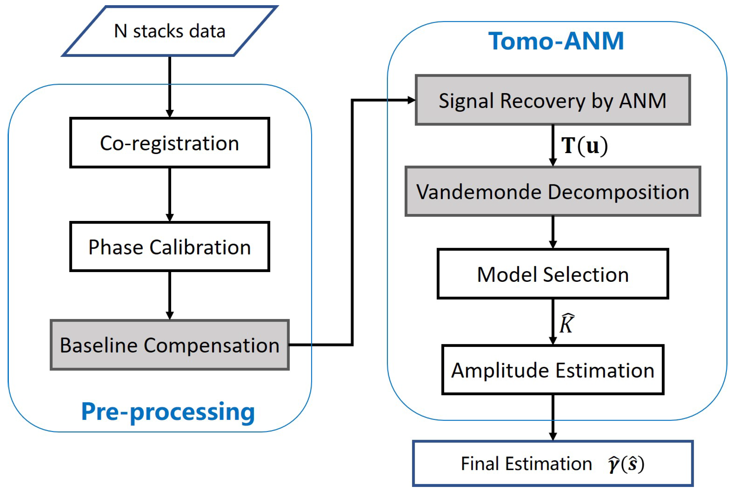
2.3. TomoSAR Algorithm Based on Atomic Norm Minimization

To invert the TomoSAR model in Equation (6), we propose a TomoSAR algorithm based on ANM, which we refer to as Tomo-ANM for convenience. The flowchart is shown in Figure 2. In the preprocessing stage, apart from the co-registration and phase calibration step, the baseline compensation step compensates randomly distributed baselines as uniform baselines or samples of uniform baselines, which is a necessary condition for using an ANM algorithm. In the TomoSAR inversion stage, the complete denoising signal is first recovered by ANM. Vandemonde decomposition is used to obtain the possible position of scatterers. We then estimate the model order—the number of scatterers—within one pixel. Finally, amplitudes of scatterers need to be reestimated by the linear inversion algorithm.

For the sake of representation, we give some definitions:

${\mathbf{b}}_{random}$: the input randomly distributed baselines;

${\mathbf{Y}}_{random}$: input N complex data;

${\mathbf{R}}_{random}$: the measurement matrix corresponding to ${\mathbf{b}}_{random}$;

${\mathbf{b}}_{\left[N\right]}$: N baselines sampled from M uniform baselines ${\mathbf{b}}_{\left[M\right]}$;

${\mathbf{Y}}_{\left[N\right]}$: incomplete noisy samples of uniform baselines data with index $\left[N\right]$;

${\mathbf{R}}_{\left[N\right]}$: the measurement matrix corresponding to ${\mathbf{b}}_{\left[N\right]}$;

${\mathbf{b}}_{\left[M\right]}$: M uniform baselines;

${\mathbf{Y}}_{\left[M\right]}$: complete denoising data of uniform baselines with index $\left[M\right]$;

${\mathbf{R}}_{\left[M\right]}$: the measurement matrix corresponding to ${\mathbf{b}}_{\left[M\right]}$.

It should be noted that $\mathbf{Y}$ in Equation (3) refers to ${\mathbf{Y}}_{random}$. A schematic diagram is given in Figure 3 to describe the data at different stages.

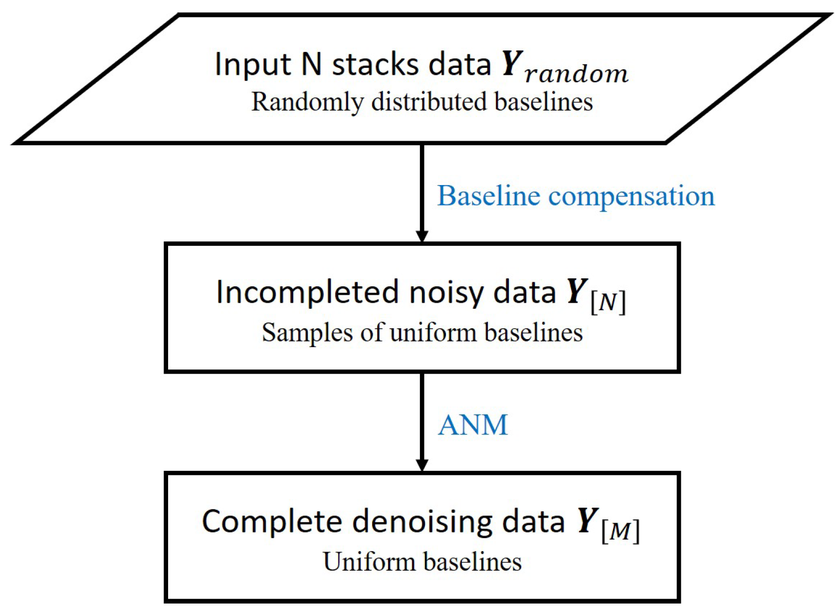
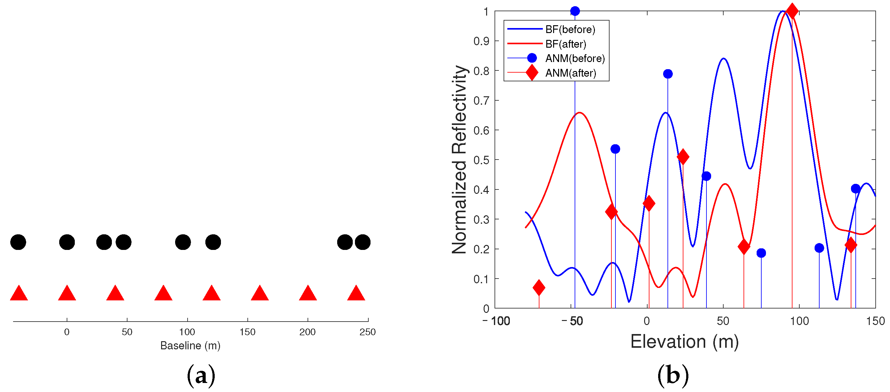
2.3.1. Baseline Compensation

In actual airborne or spaceborne cases, the N stacks TomoSAR data are usually acquired by repeat passes. Thus, the baselines are inevitably randomly distributed. The baseline compensation step compensates ${\mathbf{Y}}_{random}$ as ${\mathbf{Y}}_{\left[N\right]}$, which is the input of the ANM algorithm.

In this paper, a sector interpolation approach [21] is used to virtualize data for specific baseline position $\left[N\right]$. The compensation process can be expressed as

$${\mathbf{Y}}_{\left[N\right]}=\mathbf{H}{\mathbf{Y}}_{random}$$

(16)

where $\mathbf{H}$ is an $N\times N$ transformation matrix $(N\ge 3)$ and $\mathbf{H}$ can be found by

$$\mathbf{H}=arg\underset{\mathbf{H}}{min}\parallel vec\left\{{\mathbf{R}}_{\left[N\right]}\right\}-\mathbf{A}·vec\left\{{\mathbf{R}}_{random}\right\}{\parallel }^2$$

(17)

where $vec\{·\}$ is the vec-operator which stacks the columns of a matrix, $\mathbf{A}=diag\{\mathbf{H},\mathbf{H},\cdots ,\mathbf{H}\}$ with $\mathbf{H}$ repeated M times. The minimization problem (17) can be solved by using conventional rules for the overdetermined equation systems. In addition, the choice of ${\mathbf{b}}_{\left[N\right]}$ and ${\mathbf{b}}_{\left[M\right]}$ needs to be determined by the distribution of actual baselines ${\mathbf{b}}_{random}$.

2.3.2. Signal Recovery by ANM

The ANM algorithm can recover complete denoising signal ${\mathbf{Y}}_{\left[M\right]}$ with M uniform baselines using ${\mathbf{Y}}_{\left[N\right]},\left[N\right]\in \left[M\right]$. As we can see, there is little difference between Equation (6) to be solved and the CCS model (7). After some simple transformation, we can obtain

$$\begin{array}{cc}\hfill y_n& =\sum _{k=1}^K\gamma \left(s_k\right)exp(-j2\pi {\xi }_n{s}_k)\hfill \\ \hfill & =\sum _{k=1}^K\gamma \left(s_k\right)exp(-j2\pi ·\frac{2b_n}{\lambda r_0}·\frac{\lambda r_0}{2\mathrm{\Delta }b}·\frac{s_k}{H})\hfill \\ \hfill & =\sum _{k=1}^K\gamma \left(s_k\right)exp(-j2\pi ·\frac{b_n}{\mathrm{\Delta }b}·\frac{s_k}{H})\hfill \end{array}$$

(18)

$$\begin{array}{cc}\hfill & =\sum _{k=1}^K\gamma \left(f_k\right)exp(-j2\pi n{f}_k)f_k\in [0,1],n\in \left[N\right],\left[N\right]\in \left[M\right].\hfill \end{array}$$

(19)

Now, Equation (19) has the same form as Equation (7), which means that the TomoSAR model (6) can be solved by ANM naturally, and the complete denoising signal ${\mathbf{Y}}_{\left[M\right]}$ can be recovered from ${\mathbf{Y}}_{\left[N\right]}$ using ANM.

2.3.3. Vandemonde Decomposition

By implementing ANM, we can not only obtain recovery signal, but also obtain $\mathbf{T}\left(\mathbf{u}\right)$, which contains the frequency information of signals.

The Vandemonde decomposition of $\mathbf{T}\left(\mathbf{u}\right)$ can be computed efficiently via a subspace algorithm. We would not choose the general MUSIC or ESPERIST algorithms, which discretize the elevation into grids to obtain a measurement matrix. The root-music algorithm is a good choice for us, as it uses a polynomial method to find roots instead of the spectrum search in the MUSIC algorithm. It is not limited by the grid and can obtain more accurate results under a complete and denoising signal.

After ${\widehat{f}}_k$ is obtained, the possible elevation recovered by Vandermonde decomposition is

$${\widehat{s}}_k={\widehat{f}}_k·H.$$

(20)

where H is the unambiguous elevation.

2.3.4. Model Selection and Amplitude Estimation

Model selection, which is based on information theoretic criteria (ITC), is used to estimate the most likely number $\widehat{K}$ of point scatterers along elevation inside an azimuth-range pixel. It seeks a trade-off between model fit and complexity. In this paper, the Bayesian information criterion (BIC), an effective model selection method for TomoSAR [12,27], is chosen to estimate the proper model $\widehat{K}$. The BIC principle can be expressed as [28,29]

$$BIC\left(K\right)=-2lnp\left(\mathbf{Y}\right|\widehat{\mathbf{\theta }}\left(K\right),K)+3KlnN$$

(21)

where $\widehat{\mathbf{\theta }}\left(K\right)$ denotes the vector of amplitudes, phases, and elevation of the Kth scatterer; $p\left(\mathbf{Y}\right|\widehat{\mathbf{\theta }}\left(K\right),K)$ is the likelihood function. The number of scatterers $\widehat{K}$ and corresponding elevation $\widehat{\mathbf{s}}$ is obtained as $BIC\left(K\right)$ reaches minimization.

The previous step obtains the elevation position $\widehat{\mathbf{s}}$ under infinite dictionary. The amplitude estimation can be realized by the least-squares algorithm:

$$\widehat{\mathbf{\gamma }}\left(\widehat{\mathbf{s}}\right)={\left({\mathbf{R}}^{\mathrm{H}}\left(\widehat{\mathbf{s}}\right)\mathbf{R}\left(\widehat{\mathbf{s}}\right)\right)}^{-1}{\mathbf{R}}^{\mathrm{H}}\left(\widehat{\mathbf{s}}\right)\mathbf{Y}$$

(22)

where $\mathbf{R}\left(\widehat{\mathbf{s}}\right)$ is a $N\times \widehat{K}$ matrix with ${\mathbf{R}}_{n,\widehat{k}}\left(\widehat{\mathbf{s}}\right)=exp(-j2\pi {\xi }_n{\widehat{s}}_k)$.

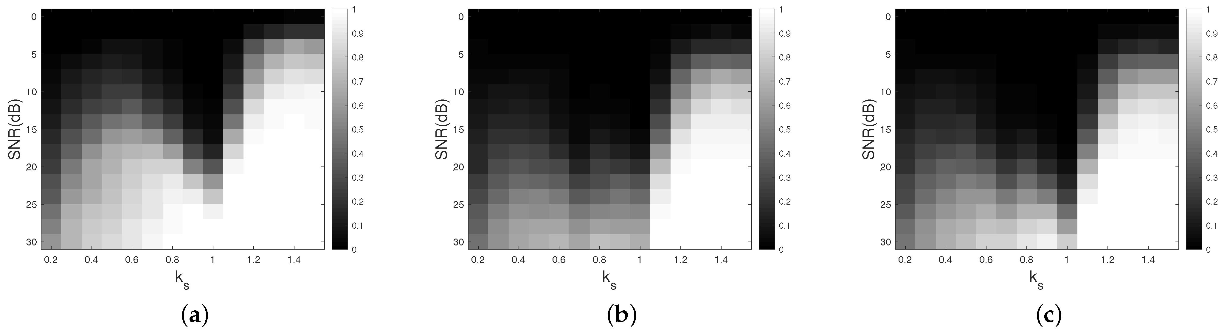
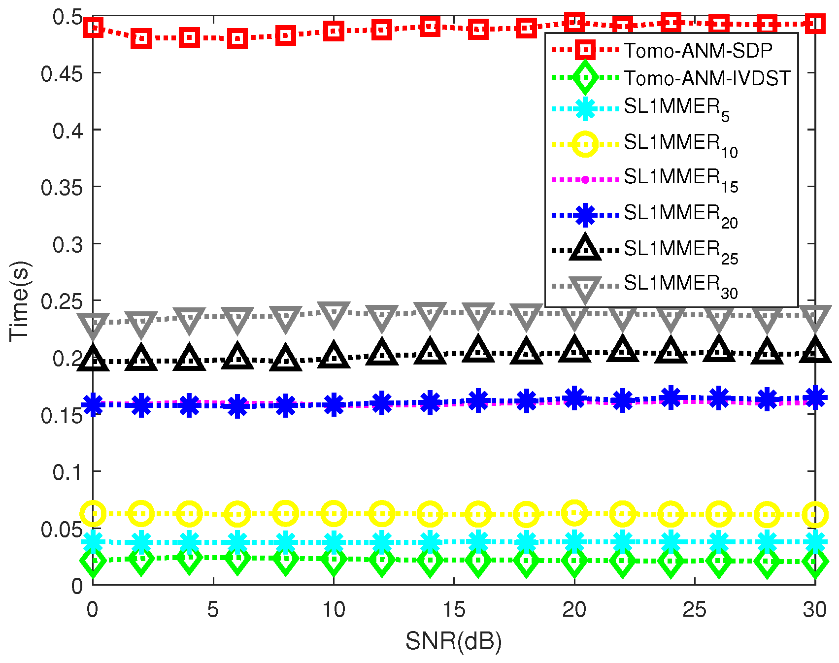
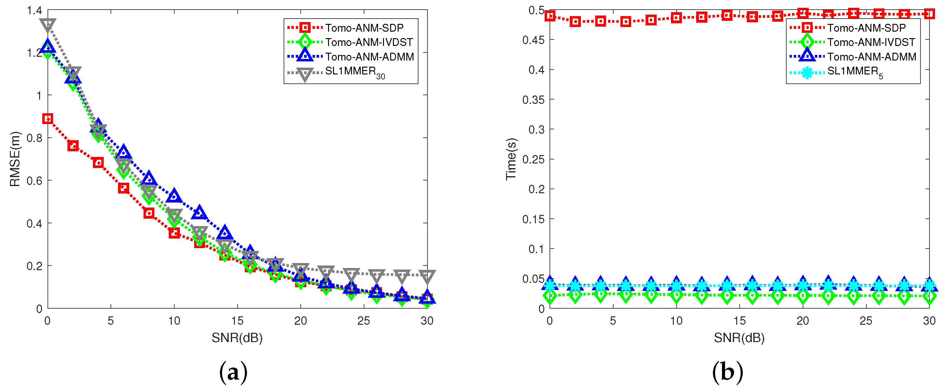
3. Simulation Results

In this section, we investigated the advantages of the proposed method by some simulation experiments. In order to show the elimination of the off-grid effect in our method, we chose SL1MMER, a typical complete framework for TomoSAR inversion proposed in [12], as a comparison. The first step of SL1MMER is “scaled down by $L_1$ norm”, which is realized by on-grid $L_1$ norm minimization.

The wavelength and slant range were set to 0.031 m and 588,303.75 m, respectively, which are equal to the parameters used in Section 4. We chose 20 samples from 32 full uniform data, with baselines shown in Figure 4. The minimum baseline is 15 m, while the maximum is 465 m. From that, the Rayleigh resolution and unambiguous height can be obtained:

$$\begin{array}{c}\hfill {\rho }_s=\frac{\lambda r}{2\mathrm{\Delta }{b}_{max}}=19.00\mathrm{m}.\end{array}$$

(23)

$$\begin{array}{c}\hfill H=\frac{\lambda r}{2\mathrm{\Delta }{b}_{min}}=607.91\mathrm{m}.\end{array}$$

(24)

Let $k_s=|s_2-s_1|/{\rho }_s$ denote the distance between two scatterer elevations $s_1$ and $s_2$. Considering the great impact of the grid density on the on-grid algorithm, we studied the performances of the SL1MMER algorithm under different numbers of grids. SL1MMER${}_{num}$ represents a grid with $num·M$ points, where M is the number of full data acquisition.

First, the removal of the off-grid effect by the Tomo-ANM algorithm is shown in Figure 5. We provide the detection results of five scatterers along the elevation direction. The black circles represent true locations, the red boxes denote the Tomo-ANM results, and the green dots show the SL1MMER detection results. Five scatterers are randomly distributed between 100 m and 105 m. The SL1MMER algorithm sets the grid interval as 1 m, and the estimation results are located at grids adjacent to the truth positions, thus producing a positioning error. Regardless of noise, Tomo-ANM can accurately obtain the scatterer positions and eliminate the off-grid effect completely. The validity of Tomo-ANM was preliminarily illustrated. Four experiments were then implemented.

Super-Resolution Capability: The super-resolution capability of Tomo-ANM, SL1MMER${}_{20}$, and SL1MMER${}_{30}$ was tested under 10 dB and 5 dB SNRs. We set two scatterers with the same amplitudes and phases, one of which was fixed at 90 m, while the other was on the right with a varying distance ($k_s=1.2,0.8,0.4$) from the first point. Both scatterers were off-grid. The results are shown in Figure 6. The top row shows the positioning results under 10 dB, and the bottom under 5 dB. From left to right, the distance between scatterers decreases. The results before model selection and amplitude estimation are shown. As we can see, the SL1MMER algorithm can only locate grids adjacent to the true position, while Tomo-ANM can position them more accurately and is not influenced by predefined grids. Regardless of the accuracy, which will be discussed next, under a 10 dB SNR, Tomo-ANM and SL1MMER can distinguish two scatterers fairly well at all distances, even when $k_s=0.4$. When the SNR is worse, $SNR=$ 5 dB in this example, scatterers can still be located well when $k_s=1.2$ and $0.8$, but with slightly more bias relative to the true position compared with $SNR=$ 10 dB. At $SNR=$ 5 dB and $k_s=0.4$, neither method can recover the two scatterers. Therefore, ANM can completely eliminate the off-grid effect and has a super-resolution capability that is no worse than that of SL1MMER.

Location Accuracy: The location accuracy of one scatterer of Tomo-ANM and SL1MMER was investigated. The SNR was set to 0:2:30 dB, and the grid density of SL1MMER was set to $num$ = 5:5:30. The elevation of the scatterer was randomly distributed in $[0,H]$, and the amplitude and phase were fixed. For each parameter setting, 1000 Monte Carlo experiments were performed. The RMSE (root mean square error) was used to measure accuracy. Results are shown in Figure 7. The accuracy of SL1MMER improves as grid density increases. For example, the RMSE falls from $0.94$ to $0.16$ m when the number of grids increases from 5 M to 30 M for $SNR=30$ dB. This proves that the off-grid effect can be alleviated to some extent in this way. The RMSE decreases quickly (from $1.33$ to $0.19$ m using $SL1MME{R}_{30}$) when the SNR changes from 0 to 20 dB, but nearly remains unchanged (from $0.19$ to $0.16$ m using $SL1MME{R}_{30}$) when the SNR is higher than 20 dB. This is because, when the SNR is good enough, the performance of SL1MMER is mainly constrained by all grids. When it comes to Tomo-ANM, the RMSE is always lower than SL1MMER under any SNR, and the difference reaches a minimum of $0.05$ m using $SL1MME{R}_{30}$ when the SNR is 16 dB. It then degrades slowly, even when the SNR exceeds 20 dB. This demonstrates that Tomo-ANM has nothing to do with grids and can obtain more accurate results than SL1MMER.

Detection Rate: The detection rate of the two scatterers using Tomo-ANM and SL1MMER was studied. The SNR was set to 0:2:30 dB, the grid density was set to $num=20,30$, and the distance between the two scatterers was set to $k_s=$ 0.2:0.1:1.5. The elevation was randomly distributed in $[0,H]$, and the amplitudes and phases were equal and fixed. We first judged whether the number of scatterers was consistent with the fact. On the premise that the number of scatterers is correct, $RMSE<threshold$ is regarded as a successful recovery; otherwise, recovery fails. In this paper, $threshold=1$ m, which is nearly 1/19${\rho }_s$. Monte Carlo experiments were performed 1000 times for each parameter setting, and the times of successful recovery were recorded to obtain the detection probability graph shown in Figure 8. The slight drop in the detection rate around $k_s=1$ is caused by the interference of the two strong scatterers. The interference effect becomes stronger when the amplitude of the scatterers becomes closer [30]. As we can see, with a higher grid density, SL1MMER${}_{30}$ performs slightly better than SL1MMER${}_{20}$. The most striking difference is that, when $K_s=0.9$ and $SNR=30$ dB, the detection rate of $SL1MME{R}_{20}$ is $72.8\%$, while that of $SL1MME{R}_{30}$ is $94.8\%$. Compared to the better-performing $SL1MME{R}_{30}$, the detection rate of Tomo-ANM is higher than SL1MMER regardless of the $K_s$ and $SNR$. For example, the detection rate of $SL1MME{R}_{30}$ is only $26.5\%$, while that of Tomo-ANM is $77.6\%$ when $K_s=1$ and $SNR=24$ dB. When $K_s=1.1$, Tomo-ANM can achieve a detection probability of more than $90\%$ when the SNR is greater than 20 dB, while $SL1MME{R}_{30}$ needs an SNR greater than 24 dB to achieve the same performance. When $K_s=1.2$, Tomo-ANM can achieve a detection probability of more than $90\%$ with an SNR greater than 14 dB, while $SL1MME{R}_{30}$ requires an SNR greater than 18 dB to achieve the same result. Therefore, Tomo-ANM performs better than SL1MMER when detecting two scatterers.

Time Consumption: The time consumption of ANM and SL1MMER was shown and analyzed. For convenience, Tomo-ANM-SDP denotes ANM realization by the SDPT3 tool, while Tomo-ANM-IVDST does so by IVDST. The $L_1$ norm minimization of SL1MMER was implemented by the iterative shrinkage-thresholding (IST) algorithm. To assess the computational efficiency of different methods, we recorded statistics on the average running time of 200 independent points under different SNRs. Only the inversion process was timed, excluding the model selection and amplitude correction steps. The simulation was performed on MATLAB 2019b on a computer equipped with an Intel Core i7 CPU @ 2.60 GHz. The results are displayed in Figure 9. There is little difference in the time of each algorithm under different SNRs, so the average time is used for time comparison below. It can be seen that the ANM algorithm implemented by SDPT3 takes an average of 0.49 s, which is the longest time. The running time of the SL1MMER algorithm increases from $0.04$ to $0.24$ s with the increase in grid density from 5 M to 30 M. There is a sudden increase when the grid density reaches 15 times. The ANM algorithm implemented by IVDST takes an average of 0.02 s, which is the shortest time and even slightly faster than the SL1MMER${}_5$ algorithm, which takes 0.04 s on average. It should be noted that the computational efficiency of Tomo-ANM-IVDST is related to parameter settings, which we discuss in Section 5.3. The computational complexity is highly related to the full data size. According to [24], the overall computational complexity of SDP is $\mathcal{O}\left(N^{3.5}\right)$ using the advanced solver SDPT3, where N represents the size of the full data, while the computational complexity of IVDST is only $\mathcal{O}\left(N^2\right)$. As shown in Figure 9, the computational efficiency improvement caused by an order of 1.5 in computational complexity reduction is considerable.

On the basis of the above simulation results, Tomo-ANM can obtain a super-resolution capability comparable to SL1MMER, has an improved location accuracy and detection rate, and is less time-consuming.

4. Real Data Results

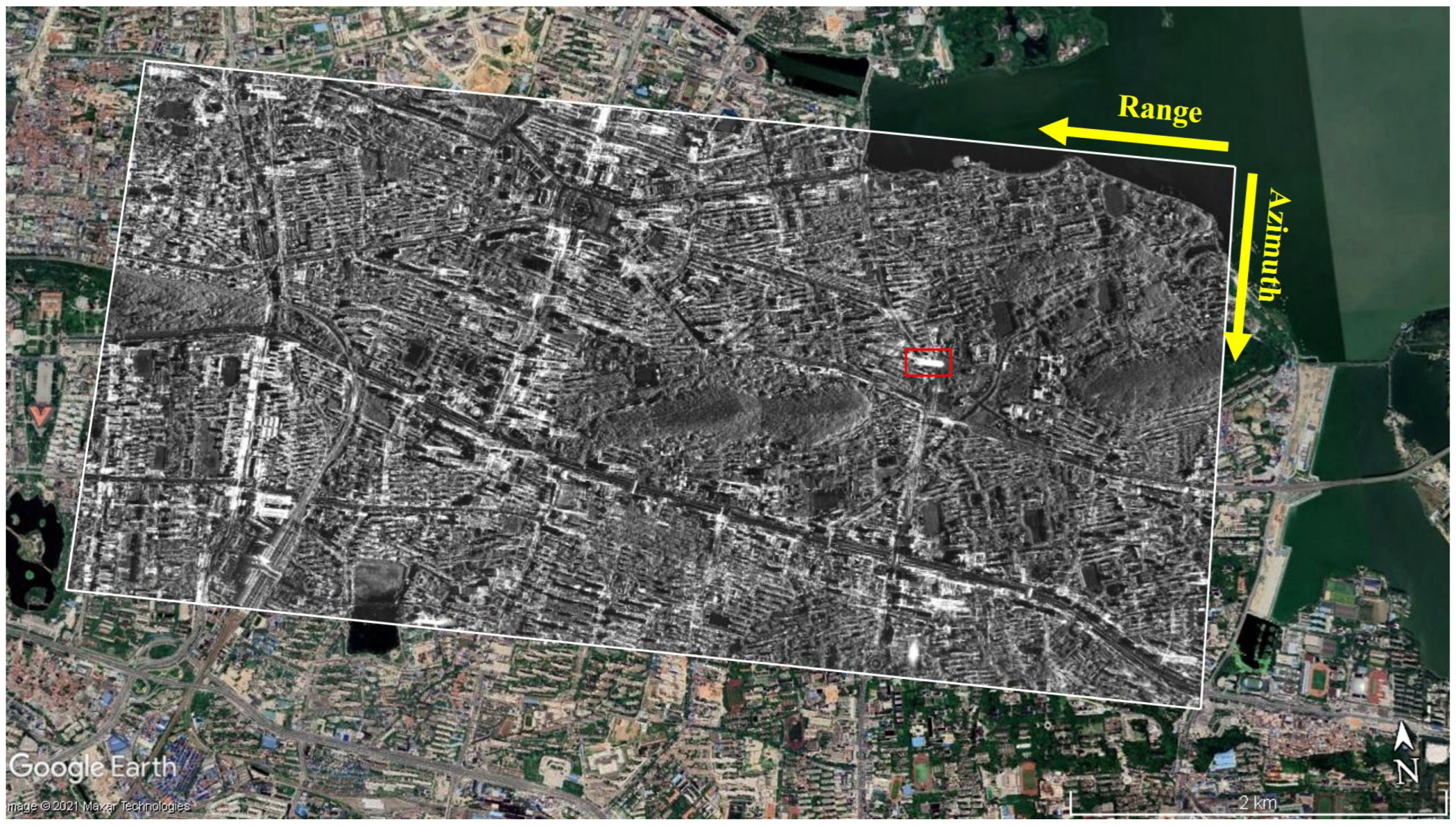
This section is devoted to demonstrating the advantages of our method, proposed in Section 2.3, in the TomoSAR inversion of urban areas using spaceborne data. We selected a high-rise building as the experimental target and verified the superiority of Tomo-ANM in removing the off-grid effect and in obtaining the building height more accurately compared with the on-grid SL1MMER algorithm.

4.1. Datasets

We utilized eight stacks staring spotlight TerraSAR-X data of the urban area of Wuhan, China, where there are many high-rise buildings. Figure 10 shows a TerraSAR image, acquired on July 2015, overlaid on Google Maps. The building marked by a red rectangle is investigated. The system parameters are shown in

Table 1. System parameters of TerraSAR-X images.

Imaging Mode	Wavelength (m)	Slant Range (m)	Incidence Angle	Range Resolution (m)	Azimuth Resolution (m)
ST	0.031	588,303.75	30.83${}^{\circ }$	0.59	0.23

. The time baseline is from June 2014 to January 2016, and the total space perpendicular baseline aperture is 285.98 m. Baseline information is reported in

Table 2. Baseline information of eight TerraSAR images.

Acquisition Date	Space Baseline (m)
28 June 2014 5 October 2014 24 May 2015 15 June 2015 29 July 2015 20 August 2015 25 October 2015 10 January 2016	245.43 30.76 230.73 121.32 0 46.90 96.25 −40.55

. Before we implement the TomoSAR inversion, some preprocessing steps, including co-registration, phase calibration, and baseline compensation, need to be carried out. Details and results of baseline compensation are given in the next section.

4.2. Results

We used images of Hubei Science and Technology Venture Building, labeled by the red box in Figure 10, to conduct the following real data experiments. Viewed from the top, the Hubei Science and Technology Venture Building is a hexagonal building, as shown in Figure 11. According to the relationship between the SAR incident direction and the building orientation, it is obvious in Figure 11a that two surfaces can be illuminated and imaged on the slant-range plane of SAR. Figure 11b is a street-view photo of Hubei Science and Technology Venture Building from Baidu Map. There are many glass windows distributed on the two illuminated surfaces of the building. At an appropriate SAR incident angle, the glasses could form strong backscattering, while the backscattering of the connected wall is relatively weak, thus forming four bright glass walls and three dark gaps in the SAR image, shown in Figure 11c.

In addition, the building has a total of 26 floors. According to multiple onsite measurements of the handheld laser rangefinder at different angles, the building height is 99 m [27].

4.2.1. Baseline Compensation

The baseline compensation step virtualizes the data at uniform baselines or the sampling data of uniform baselines based on the existing non-uniform baselines and data. In this paper, we employed the sector interpolation approach [21], explained in detail in Section 2.3.1. When determining the uniform baselines ${\mathbf{b}}_{\left[M\right]}$ to be compensated, the minimum baseline and baseline aperture of the real non-uniform perpendicular baseline should be taken into full consideration, so as to make the virtual baseline position close to the original baseline position as much as possible and maximize the use of existing data.

In this case, we set the uniform baselines as −40:40:240 m, shown in Figure 12a. Thus, the Rayleigh resolution and unambiguous height are 28.55 m and 228.45 m, respectively. A point, marked in red in Figure 11c, in the middle and upper part of the building was selected to demonstrate the necessity of baseline compensation. For the convenience of presentation, we first give the spectrum inversion results of beamforming before and after baseline composition, shown by the blue and red line in Figure 12b, respectively. In both cases, the position of the scatterer at about 100 m is obtained, but the maximum sidelobe amplitude is suppressed after baseline compensation. The ANM algorithm requires uniform baselines or sampling of uniform baselines. If non-uniform baseline data are directly input into the ANM inversion algorithm, it will obtain wrong results due to uneven baselines, shown by the blue circle in Figure 12b. After using the sector interpolation approach to compensate baselines, the correct elevation position can be retrieved, shown by the red diamond in Figure 12b. Hence, baseline compensation is a necessary step for Tomo-ANM.

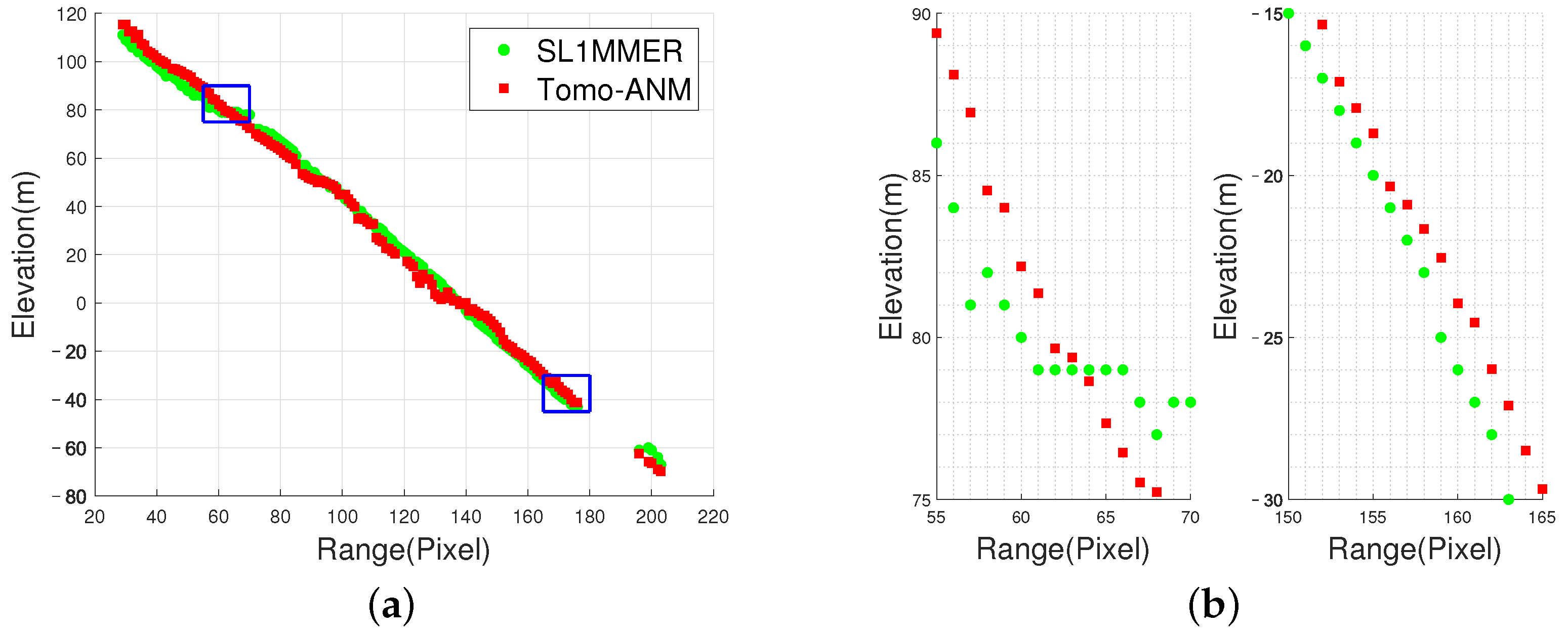
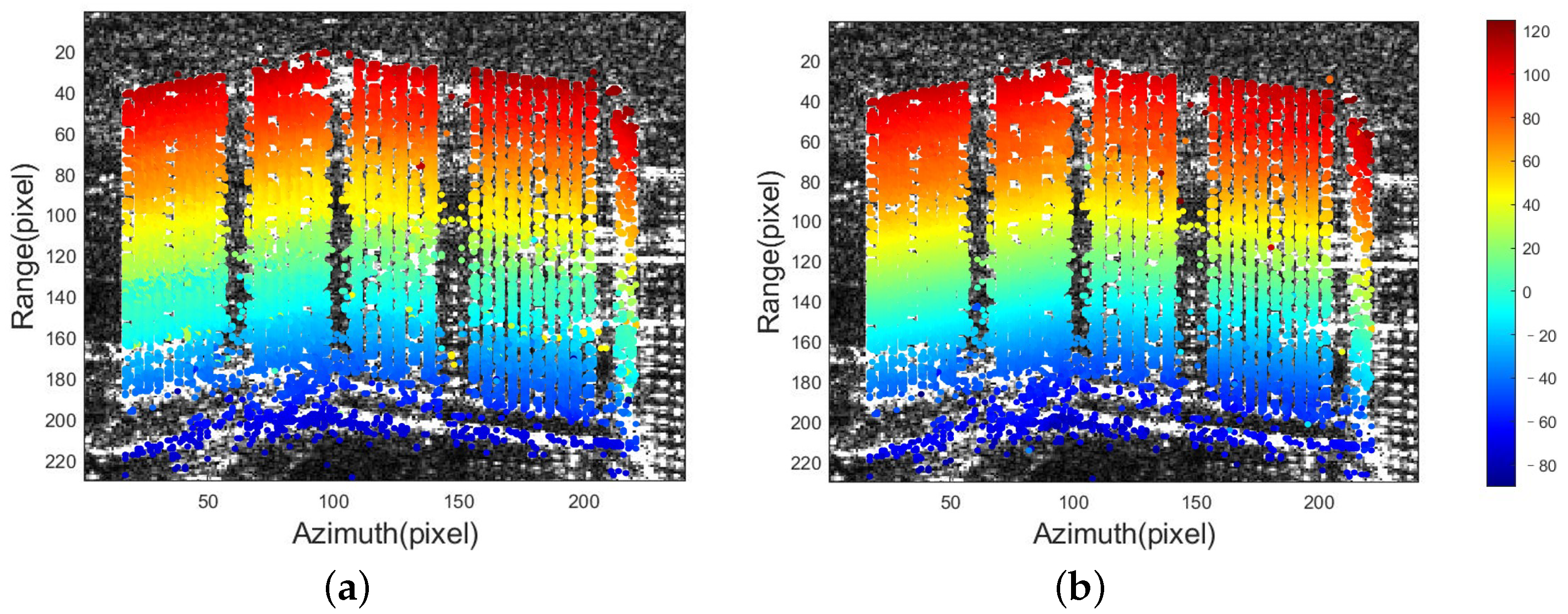
4.2.2. Tomographic Profiles

In order to observe the influence of the off-grid effect, we selected a line target with an azimuth number of 69, shown in Figure 11c with a blue line, to display the tomographic profiles. For SL1MMER, the grid interval was set as 1 m, which is nearly 1/19 of the Rayleigh resolution. Figure 13 shows the reconstruction profiles of the test line in the elevation and range direction. SAR illuminates from the left to the right of the scene. The roof is at a near distance, while the floor is at a far distance. The height changes continuously and increases gradually from the floor to the roof. The results of Tomo-ANM and SL1MMER in Figure 13a are both consistent with the above description, i.e., our expectations. To better show the reconstruction details, we provide an enlargement of the blue box in Figure 13a,b, using the same markers as Figure 13a. It can be seen that the results of the SL1MMER algorithm (green points) are firmly restricted by the grids with 1 m intervals shown by the dashed line in the background, especially at range pixels 60 to 66, which affects the fine characterization of the target’s 3D structure. Tomo-ANM profiles are distributed continuously in the entire elevation space and are not constrained by the grid; thus, they can better ensure the continuity of the building facade and achieve the fine characterization of targets.

By comparing the two tomographic profiles shown in Figure 13, due to the off-grid effect, the on-grid TomoSAR inversion–SL1MMER profiles are influenced by the grids, while the Tomo-ANM profiles, using continuous dictionary, eliminate the off-grid effect completely and can better position the scatterers.

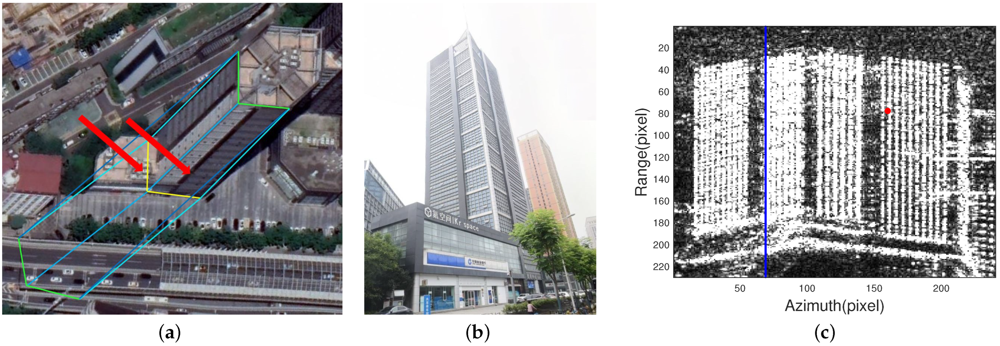
4.2.3. Height Estimation of the Building

To demonstrate the validity and potential of the Tomo-ANM method for urban area analysis, we implemented tomographic inversion on the whole test building in Figure 11c. Figure 14 shows the reconstruction results overlaid on an amplitude image, with different colors representing elevation values. Note that the elevation value shown is at an elevation direction perpendicular to the azimuth-range plane and does not transform from the elevation coordinate to the height coordinate perpendicular to the ground. By comparing Figure 14a,b intuitively, it is obvious that both algorithms can recover the general elevation change of the building, and the elevation trend is correct.

We chose five pairs of points from the reconstruction results of the building for height estimation. Each pair of points is one point on the roof and one on the floor. For the convenience of comparing the results with the real building height, the elevation values of each pair were converted into height values. The building height estimated by each pair of points and the final building height estimation of each method are given in

Table 3. Height estimation of different methods.

	Height 1 (m)	Height 2 (m)	Height 3 (m)	Height 4 (m)	Height 5 (m)	Average Height (m)	Estimation Error
Tomo-ANM-SDP	96.28	96.02	96.32	96.95	97.52	96.62	$2.40\%$
Tomo-ANM-IVDST	96.10	94.56	97.33	94.26	96.25	95.70	$3.33\%$
SL1MMER	92.25	93.79	92.25	90.20	90.71	91.84	$7.23\%$

. Based on comparisons with the true height of the building, 99 m, the building height estimated by the Tomo-ANM-SDP algorithm is 96.62 m and has only a $2.40\%$ error, which is the most accurate elevation estimation result. The estimation error of Tomo-ANM-IVDST is $3.33\%$, which shows comparable estimation accuracy [24] with Tomo-ANM-SDP. The height estimated by SL1MMER is 91.84 m, and the estimation error is $7.23\%$, $4.83\%$ higher than Tomo-ANM-SDP. Therefore, using Tomo-ANM improves the accuracy of building height estimation in the tomographic reconstruction in urban areas, because the off-grid effect is eliminated.

The running time of Tomo-ANM-SDP, Tomo-ANM-IVDST, and SL1MMER of the whole building are 1.4 h, 1.4 min, and 8.1 min, respectively.

5. Discussion

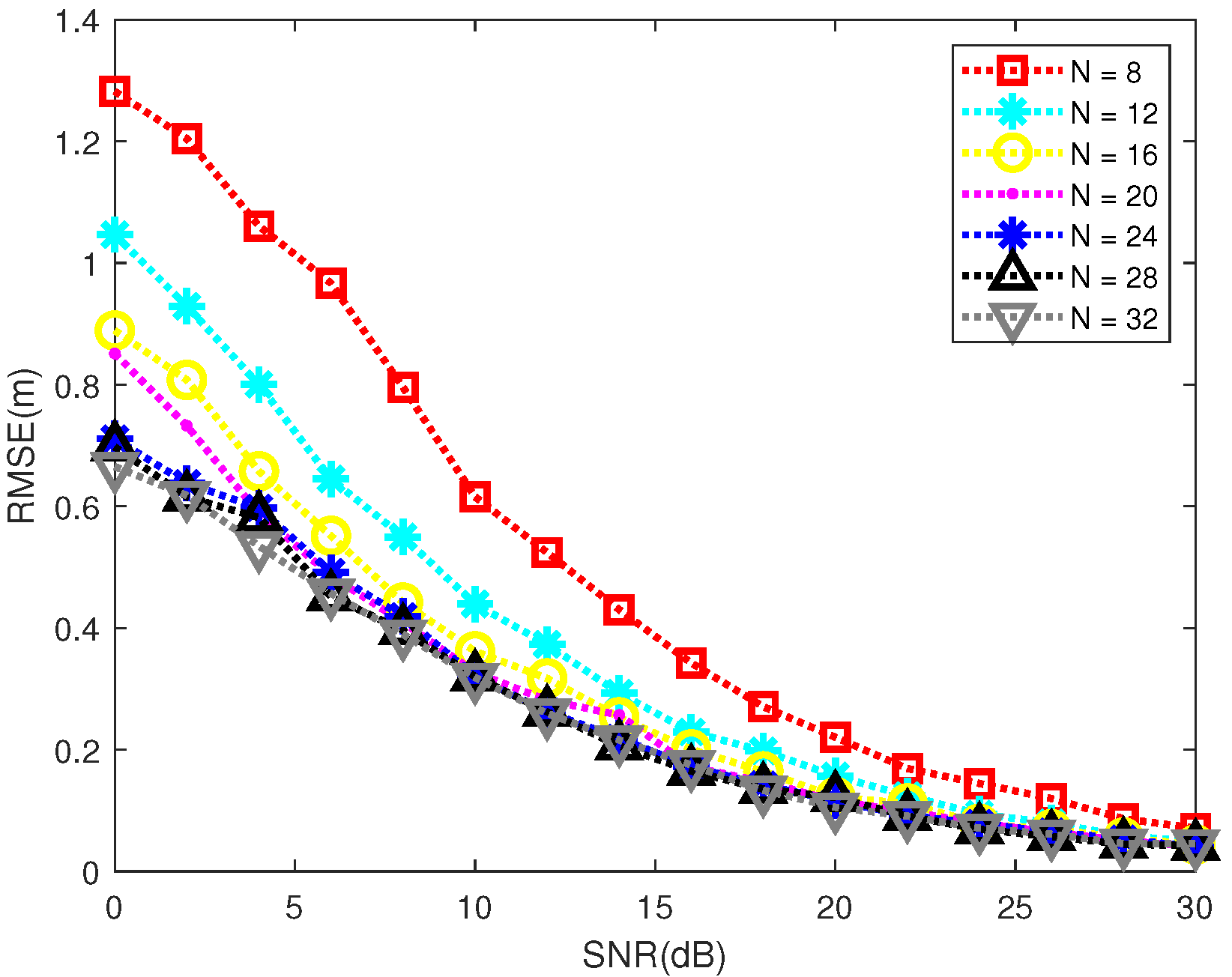
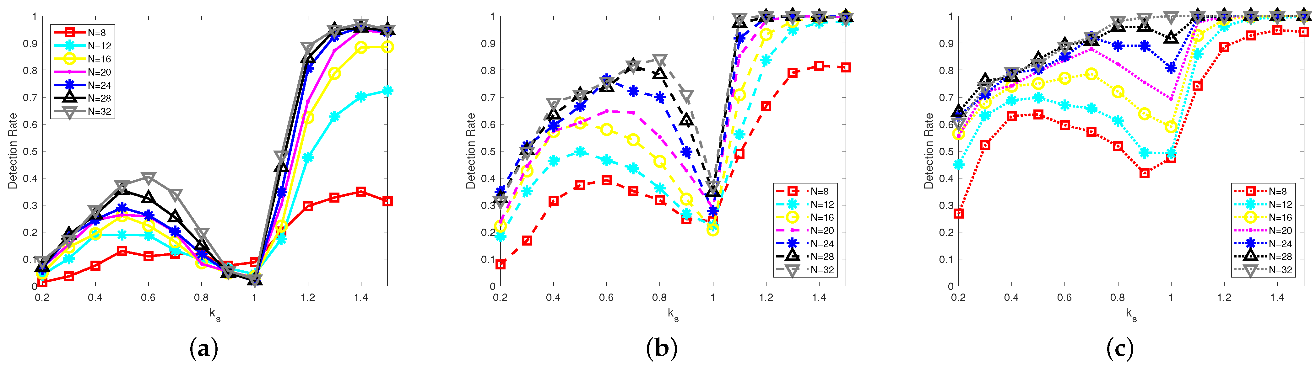
5.1. Performance of Tomo-ANM under Different Samples

As mentioned above, ANM can recover a denoising complete signal ${\mathbf{Y}}_{\left[M\right]}$ from a noisy incomplete signal ${\mathbf{Y}}_{\left[N\right]}$. In this section, we discuss the location accuracy and detection rate of Tomo-ANM under different samples N. The parameter settings were the same as those in Section 3, and N = 8:4:32 when full sample M = 32. For every parameter setting, 1000 Monte Carlo experiments were carried out. Results are shown in Figure 15 and Figure 16.

Figure 15 displays the change in RMSE with the SNR under different sample numbers N. The accuracy of Tomo-ANM under every N increases with the increase in SNR. This is consistent with the conclusion in Section 3. With the increase in the sampling rate, the positioning increases in accuracy. The RMSE decreases from $1.28$ to 0.67 m, while N changes from 8 to 32 with SNR set to 0 dB. When N is greater than 20, the positioning accuracies are very close to each other. Even at $N=8$, the positioning accuracy with a good SNR, 0.07 m at 30 dB, is very competitive. Figure 16 shows the performance of the detection rate of the two scatterers under different N and SNR values. The horizontal axis is the normalized distance, and the vertical axis is the detection rate. The performance under three SNRs (10 dB, 20 dB, 30 dB) is presented by different line types, respectively, in Figure 16a–c, and the performance of different sample numbers N was studied under each SNR. There is still a drop around $k_s=1$. When N is fixed at 8 and $k_s=1.6$, the detection rate is $30.8\%$ at 10 dB, $83.4\%$ at 20 dB, and $94.2\%$ at 30 dB; that is to say, the better the SNR, the higher the detection rate. Under the same SNR, the higher the sample number N is, the better the detection rate is. For instance, detection rate increases from $65\%$ to $100\%$ as N grows from 8 to 32 when $k_s=1.2$. Likewise, when N is greater than 20, the detection rates are close at different $k_s$ values except when $k_s$ is around 1.

Therefore, the performance of Tomo-ANM, both in positioning accuracy and detection rate, decreases with a decrease in the sample number N. However, when N is greater than 20, that is, when the sampling rate is greater than 62.5%, the performance of Tomo-ANM is relatively close, and there is no great improvement as N increases in most cases.

5.2. Comparison between IVDST and ADMM

As stated in Section 1, ADMM is a mature algorithm widely used in SDP acceleration [22,23,31,32]. In this section, we made a simple comparison of two fast implementations of ANM, IVDST, and ADMM. The parameter settings were the same as those in Section 3. Results are shown in Figure 17.

Figure 17a displays the location accuracy of Tomo-ANM-IVDST and Tomo-ANM-ADMM, with Tomo-ANM-SDP and SL1MMER${}_{30}$ as a contrast. When $SNR<$ 10 dB, the position accuracy of Tomo-ANM-IVDST is slightly better (0.02 m lower for $SNR=10$ dB) than that of the on-grid algorithm SL1MMER${}_{30}$. When $SNR>$ 10 dB, the accuracy of Tomo-ANM-IVDST gradually becomes better than SL1MMER${}_{30}$ and is close to that of Tomo-ANM-SDP. The RMSE values of Tomo-ANM-IVDST and Tomo-ANM-SDP are the same, 0.04 m, when $SNR=30$ dB. For Tomo-ANM-ADMM, the accuracy is superior or close to SL1MMER${}_{30}$ when $SNR<$ 4 dB. When SNR is between 6 dB and 14 dB, the accuracy of Tomo-ANM-ADMM is slightly inferior (0.08 m higher at $SNR=12$ dB) to SL1MMER${}_{30}$. When $SNR>$ 20 dB, the accuracy of Tomo-ANM-ADMM is comparable to that of Tomo-ANM-SDP. To sum up, the location accuracy of Tomo-ANM-IVDST is always superior to Tomo-ANM-ADMM. The accuracy of both fast realizations is comparable to Tomo-ANM-SDP at a high SNR. Figure 17b shows the running time of Tomo-ANM-IVDST and Tomo-ANM-ADMM, with Tomo-ANM-SDP and SL1MMER${}_5$ as a reference. As we can see, both algorithms can significantly reduce running time relative to Tomo-ANM-SDP. The time consumption of Tomo-ANM-ADMM (0.04 s on average) is equivalent to that of SL1MMER${}_5$, while Tomo-ANM-IVDST is slightly more effective than SL1MMER${}_5$. It is worth noting that the time of Tomo-ANM-ADMM is closely related to the parameter setting. In order to obtain reliable results, 30–50 iterations are carried out in this paper.

For further verification, we also compared the two fast algorithms on the real data. The same five pairs of points as in Section 4.2.3 were selected for building height estimation. The results and running time are shown in

Table 4. Height estimation of Tomo-ANM-IVDST and Tomo-ANM-ADMM.

	Height Estimation (m)	Estimation Error	Running Time (min)
Tomo-ANM-IVDST	95.70	$3.33\%$	1.4
Tomo-ANM-ADMM	94.10	$4.95\%$	1.7

. It can be seen that the building height estimation result of Tomo-ANM-IVDST (95.70 m) is slightly better than Tomo-ANM-ADMM (94.10 m) and takes less time.

By comparison, Tomo-ANM-IVDST can achieve better location accuracy in less time than Tomo-ANM-ADMM. This is why we choose IVDST as the fast implementation of ANM in this paper.

5.3. Parameter Settings of Tomo-ANM

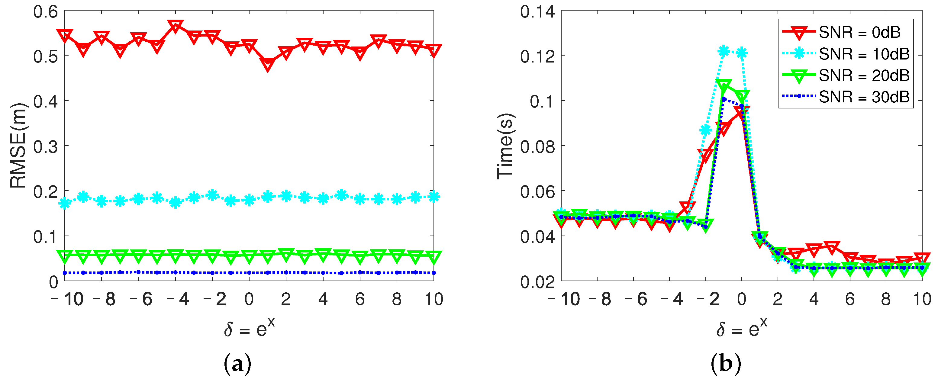
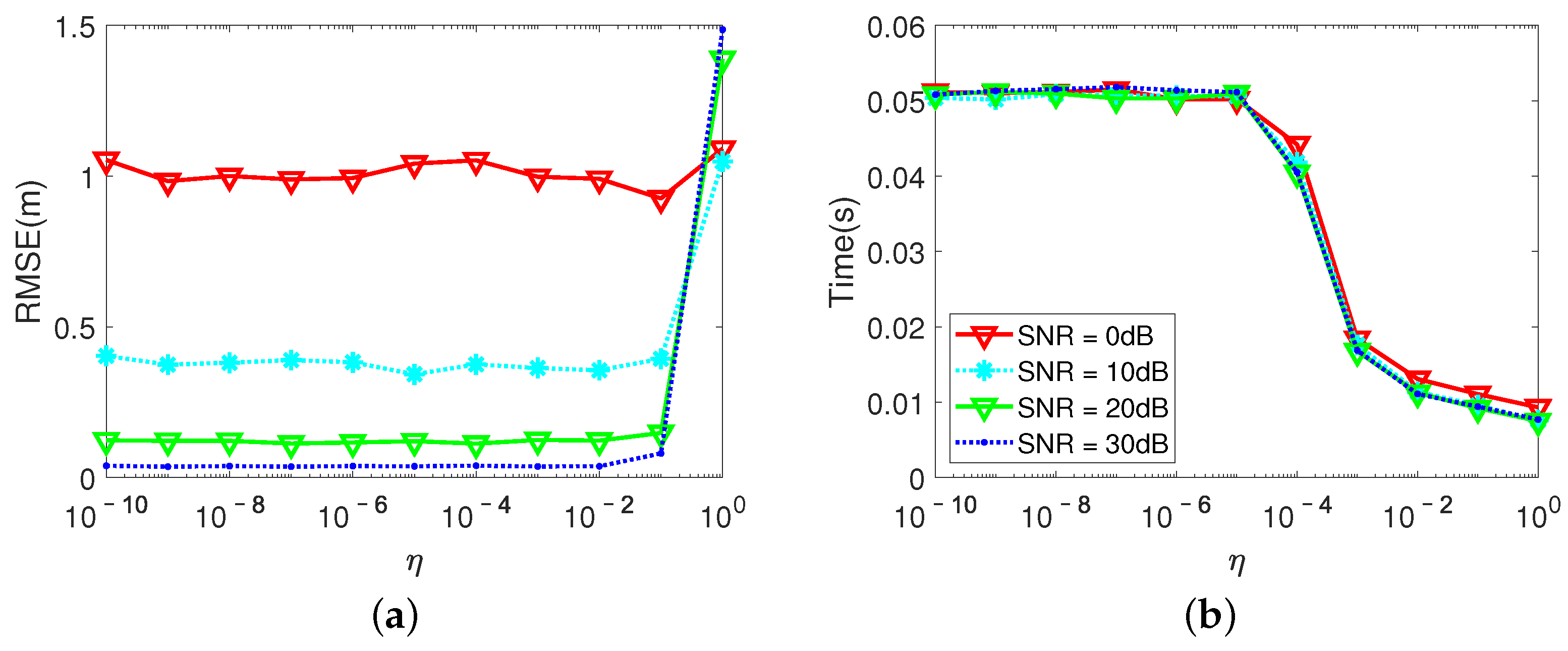
There is one parameter to be input in the Tomo-ANM-SDP, and three parameters in the Tomo-ANM-IVDST. These parameters need to be set manually at present. In this section, we discuss the range and impact of Tomo-ANM parameter settings.

5.3.1. Tomo-ANM-SDP

In Section 2.2, we introduced the theory of ANM in detail. The regularization parameter $\tau$ needs to be input. According to the authors in [22], the choice of regularization parameter is dictated by the noise model. They show the lower and higher bound of $\tau$ under Gaussian noise. The lower bound whenever $N⩾5$ is

$$\sigma \sqrt{Nlog\left(N\right)-\frac{N}{2}log\left(4\pi log\left(N\right)\right)}$$

(25)

The upper bound for $N>3$ is

$$\sigma (1+\frac{1}{log\left(N\right)})\sqrt{Nlog\left(N\right)+Nlog\left(4\pi log\right(N\left)\right)}$$

(26)

where $\sigma$ is the noise variance. In the simulation experiment, $\tau$ can be selected according to the above range. However, when processing the real data, it is necessary to obtain appropriate parameters through multiple attempts since the noise variance $\sigma$ is difficult to exactly estimate from the incomplete noisy data [33].

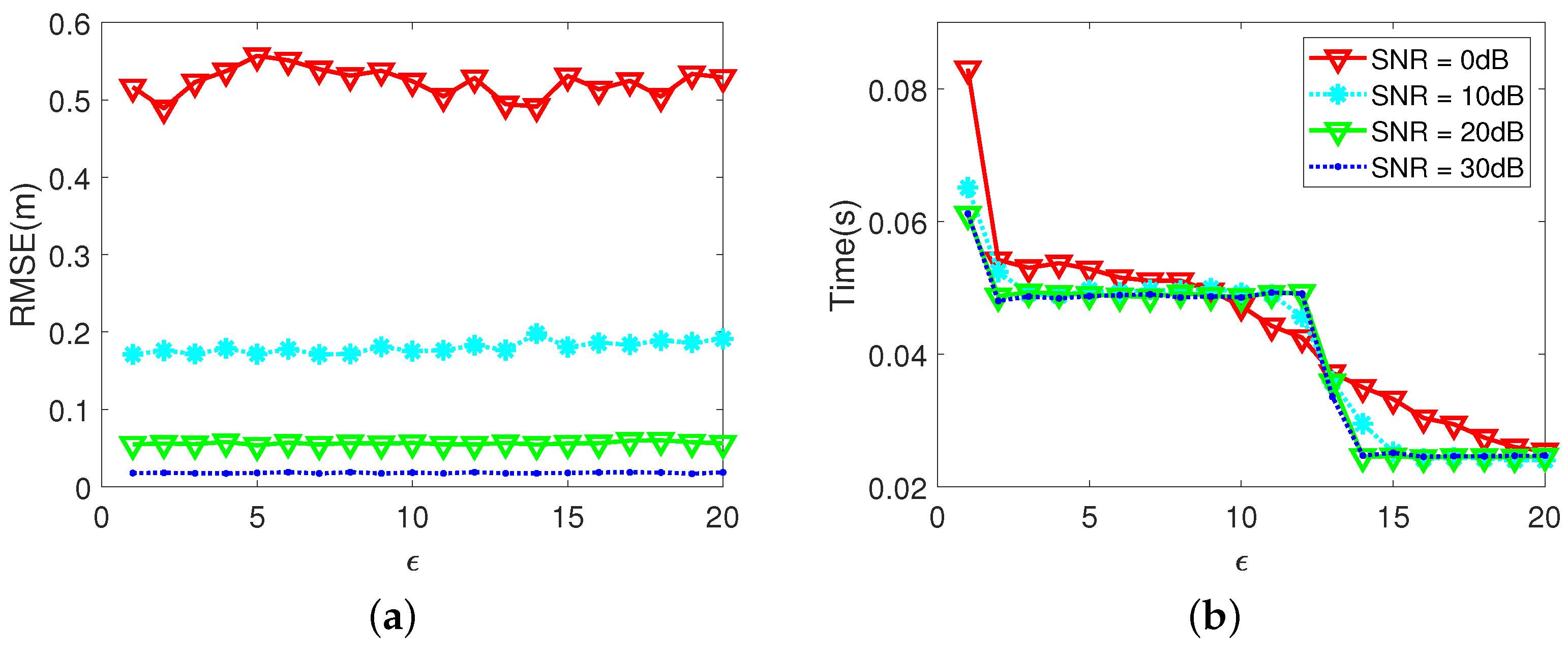
5.3.2. Tomo-ANM-IVDST

As mentioned in Section 2.2, IVDST is an iterative and shrinkage-thresholding algorithm. Three parameters need to be set before iterations [24]. They are stepsize $\delta$, shrinkage-threshold $ϵ$, and stopping criterion $\eta$. The parameter setting of the system is the same as Section 3. Three hundred Monte Carlo experiments are implemented for each parameter setting, and the maximum number of iterations was set to 30.

Stepsize $\delta$ represents the change in variables along the gradient direction from one iteration to the next. In this paper, the change in stepsize was set to $\delta =e^x$ with $x=-$10:1:10. The RMSE and time were obtained, as shown in Figure 18a,b. It can be seen that the accuracy of Tomo-ANM-IVDST under different SNRs almost does not change with $\delta$. Overall, the time consumption decreases with the increase in $\delta$, from 0.04 s when $\delta =e^{-10}$ to 0.02 s when $\delta =e^{10}$. The computational efficiency is similar for different SNRs. It is worth noting that when stepsize $\delta$ is around $e^{-1},e^0$, the time consumption surges to more than 0.1 s. Checking the number of iterations, we found that some experiments reached the maximum number of iterations we set. This is because the change in objective function is not monotonically decreasing, but it increases slowly after reaching the minimum value. These stepsize values were not set reasonably, resulting in the value of the objective function fluctuating near the minimum value and failing to reach the stop condition. Fortunately, the accuracy of Tomo-ANM-IVDST is not greatly affected. Therefore, the stepsize $\delta$ setting affects the time consumption, which needs to be adjusted by several times to obtain the appropriate value.

The shrinkage-threshold $ϵ$ is used to shrink the small diagonal values of $\Lambda$, which denotes a diagonal matrix obtained by SVD decomposition of $\mathbf{T}\left(\mathbf{u}\right)$, thus enforcing low-rankness on $\mathbf{T}$. We set $ϵ=$ 1:1:20 in this paper, and the results of the RMSE and time under different SNRs are shown in Figure 19a,b. Still, the accuracy of Tomo-ANM-IVDST is not affected by $ϵ$. The time decreases from $0.06$ to 0.02 s when $ϵ$ changes from 1 to 20 at 30 dB. That is to say, setting $ϵ$ to a small value would increase the running time. Reasonably increasing the value of $ϵ$ can improve computation speed. However, if $ϵ$ is too large, it may affect the determination of the number of scatterers. Therefore, $ϵ$ needs to be set appropriately according to the value of the singular values of the $\mathbf{T}$ matrix and the number of possible scatterers.

The stopping criterion $\eta$ is a predefined precision of the residual $\parallel {\mathbf{T}}_{i+1}-{\mathbf{T}}_i{\parallel }_F/{\parallel {\mathbf{T}}_i\parallel }_F$, where i represents iteration times. To better illustrate the impact of the change in $\eta$, we set $\eta$ so that it changes from ${10}^{-10}$ to ${10}^0$. In practice, $\eta ={10}^0$ is usually not set because reliable results cannot be obtained. The results of the RMSE and time consumption are shown in Figure 20a,b. As we can see, when $\eta \le {10}^{-2}$, the accuracy of Tomo-ANM-IVDST under different SNRs performs well and does not change very much. However, there is a large increase (from $0.04$ to 1.49 m at $SNR=30$ dB) when $\eta$ increases from ${10}^{-2}$ to ${10}^0$. Looser stop criterions lead to lower positioning accuracy. In Figure 20b, time consumption at different SNRs is almost the same. Time decreases from $0.05$ to 0.01 s while $\eta$ changes from ${10}^{-10}$ to ${10}^0$ at 30 dB. A sudden decrease (from $0.05$ to 0.01 s) occurs when $\eta$ increases from ${10}^{-5}$ to ${10}^{-2}$ at 30 dB, which means looser stop criterions can be achieved with fewer iterations. Note that the number of iterations reaches the maximum we set when $\eta \le {10}^{-5}$, so the running time is limited. It actually takes longer to reach the stop criterion. Combined with the accuracy performance, $\eta$ can be selected for a higher accuracy obtained in a shorter time. In this paper, $\eta$ can be ${10}^{-2}$ or ${10}^{-3}$. The choice of $\eta$ needs to be determined after many attempts.

To sum up, the parameter settings of Tomo-ANM require multiple attempts to obtain appropriate values. Parameter settings have a great impact on accuracy and time consumption, especially for Tomo-ANM-IVDST. In the future, we will try to study the adaptive selection of ANM parameters to facilitate its application in tomography.

6. Conclusions

In order to eliminate the off-grid effect, this paper proposes an SAR tomography algorithm based on ANM, a continuous compressed sensing algorithm, named Tomo-ANM. To meet the baseline requirements of ANM, we first performed baseline compensation to obtain uniform baselines or uniform baseline sampling data. Next, the noisy incomplete data were restored to noise-free complete data by the ANM algorithm, and the generated matrix $\mathbf{T}\left(\mathbf{u}\right)$ contained the signal frequency information. The possible scatterer elevation positions can be found by Vandermonde decomposition of the $\mathbf{T}\left(\mathbf{u}\right)$ matrix. The final estimation result was obtained through model selection and amplitude estimation. To increase the computational speed, a fast ANM algorithm named IVDST was employed.

Simulation experiments implied that Tomo-ANM can eliminate the off-grid effect completely and obtain a super-resolution capability comparable to SL1MMER. Compared with the conventional on-grid algorithm, Tomo-ANM can obtain more accurate single-scatterer positioning accuracy and higher double-scatterer detection probability. The fast ANM algorithm IVDST can reduce computational complexity by an order of 1.5 and greatly improve the algorithm availability. We also used eight stacks TerraSAR staring spotlight data to conduct real data experiments. The results showed that, compared with the on-grid algorithm, Tomo-ANM can eliminate the off-grid effect, so as to better position scatterers and obtain more accurate building height estimation results.

We analyzed the effect of the sampling rate on ANM, and the results showed that a sampling rate of 62.5% can guarantee good results, while increasing sampling on this basis cannot achieve any significant improvement in most cases. Moreover, we choose IVDST as ANM’s fast realization for its superior performance in comparison to ADMM. Parameter settings have a great impact on the performance of Tomo-ANM, especially Tomo-ANM-IVDST. At present, we can only manually select appropriate parameters after multiple attempts. Next, we will consider studying adaptive parameter selection.

This paper is an attempt to use a continuous compressed sensing algorithm for TomoSAR inversion, which preliminarily illustrates the availability and effectiveness of continuous compressed sensing in tomographic reconstruction. Many other continuous compressed sensing algorithms also have good characteristics. For example, better super-resolution capabilities can be obtained through reweighted atomic norm minimization (RAM) [34,35], and gridless SPICE (GLS) [23] can be used to eliminate the dependence on noise level parameter estimation. It is worth looking into what role these algorithms will play in TomoSAR 3D scene reconstruction and what effect they will have.

References

1. Reigber, A.; Moreira, A. First demonstration of airborne SAR tomography using multibaseline L-band data. IEEE Trans. Geosci. Remote Sens. 2000, 38, 2142–2152. [Google Scholar] [CrossRef]
2. She, Z.; Gray, D.; Bogner, R.; Homer, J. Three-dimensional SAR imaging via multiple pass processing. In Proceedings of the IEEE 1999 International Geoscience and Remote Sensing Symposium. IGARSS’99 (Cat. No.99CH36293), Hamburg, Germany, 28 June–2 July 1999; Volume 5, pp. 2389–2391. [Google Scholar] [CrossRef]
3. Sauer, S.; Ferro-Famil, L.; Reigber, A.; Pottier, E. Three-Dimensional Imaging and Scattering Mechanism Estimation Over Urban Scenes Using Dual-Baseline Polarimetric InSAR Observations at L-Band. IEEE Trans. Geosci. Remote Sens. 2011, 49, 4616–4629. [Google Scholar] [CrossRef] [Green Version]
4. Lombardini, F.; Reigber, A. Adaptive spectral estimation for multibaseline SAR tomography with airborne L-band data. In Proceedings of the IGARSS 2003—2003 IEEE International Geoscience and Remote Sensing Symposium (IEEE Cat. No.03CH37477), Toulouse, France, 21–25 July 2003; Volume 3, pp. 2014–2016. [Google Scholar] [CrossRef]
5. Gini, F.; Lombardini, F. Multibaseline cross-track SAR interferometry: A signal processing perspective. IEEE Aerosp. Electron. Syst. Mag. 2005, 20, 71–93. [Google Scholar] [CrossRef]
6. Guillaso, S.; Reigber, A. Scatterer characterisation using polarimetric SAR tomography. In Proceedings of the 2005 IEEE International Geoscience and Remote Sensing Symposium, IGARSS’05, Seoul, Korea, 29 July 2005; Volume 4, pp. 2685–2688. [CrossRef]
7. Fornaro, G.; Lombardini, F.; Serafino, F. Three-dimensional multipass SAR focusing: Experiments with long-term spaceborne data. IEEE Trans. Geosci. Remote Sens. 2005, 43, 702–714. [Google Scholar] [CrossRef]
8. Zhu, X.X.; Bamler, R. Tomographic SAR Inversion by L1 -Norm Regularization—The Compressive Sensing Approach. IEEE Trans. Geosci. Remote Sens. 2010, 48, 3839–3846. [Google Scholar] [CrossRef] [Green Version]
9. Budillon, A.; Evangelista, A.; Schirinzi, G. Three-Dimensional SAR Focusing From Multipass Signals Using Compressive Sampling. IEEE Trans. Geosci. Remote Sens. 2011, 49, 488–499. [Google Scholar] [CrossRef]
10. Dong, X.; Zhang, Y. A Novel Compressive Sensing Algorithm for SAR Imaging. IEEE J. Sel. Top. Appl. Earth Obs. Remote Sens. 2014, 7, 708–720. [Google Scholar] [CrossRef]
11. Kang, M.S.; Kim, K.T. Compressive Sensing Based SAR Imaging and Autofocus Using Improved Tikhonov Regularization. IEEE Sens. J. 2019, 19, 5529–5540. [Google Scholar] [CrossRef]
12. Zhu, X.X.; Bamler, R. Super-Resolution Power and Robustness of Compressive Sensing for Spectral Estimation With Application to Spaceborne Tomographic SAR. IEEE Trans. Geosci. Remote Sens. 2012, 50, 247–258. [Google Scholar] [CrossRef]
13. Chi, Y.; Scharf, L.L.; Pezeshki, A.; Calderbank, A.R. Sensitivity to Basis Mismatch in Compressed Sensing. IEEE Trans. Signal Process. 2011, 59, 2182–2195. [Google Scholar] [CrossRef]
14. Tang, G.; Bhaskar, B.N.; Shah, P.; Recht, B. Compressed Sensing Off the Grid. IEEE Trans. Inf. Theory 2013, 59, 7465–7490. [Google Scholar] [CrossRef] [Green Version]
15. Candès, E.J.; Fernandez-Granda, C. Towards a Mathematical Theory of Super-Resolution. Commun. Pure Appl. Math. 2012, 67, 906–956. [Google Scholar] [CrossRef] [Green Version]
16. Lei, Y.; Zhou, J.; Xiao, H. Super-resolution radar imaging using fast continuous compressed sensing. Electron. Lett. 2015, 51, 2043–2045. [Google Scholar] [CrossRef]
17. Tang, W.G.; Jiang, H.; Pang, S.X. Grid-Free DOD and DOA Estimation for MIMO Radar via Duality-Based 2D Atomic Norm Minimization. IEEE Access 2019, 7, 60827–60836. [Google Scholar] [CrossRef]
18. Feng, W.; Guo, Y.; Zhang, Y.; Gong, J. Airborne radar space time adaptive processing based on atomic norm minimization. Signal Process. 2018, 148, 31–40. [Google Scholar] [CrossRef]
19. Su, Y.; Wang, T.; Tao, F.; Li, Z. A Grid-Less Total Variation Minimization-Based Space-Time Adaptive Processing for Airborne Radar. IEEE Access 2020, 8, 29334–29343. [Google Scholar] [CrossRef]
20. Bao, Q.; Han, K.; Lin, Y.; Zhang, B.; Liu, J.; Hong, W. Imaging method for downward-looking sparse linear array three-dimensional synthetic aperture radar based on reweighted atomic norm. J. Appl. Remote Sens. 2016, 10, 015008. [Google Scholar] [CrossRef]
21. Lombardini, F.; Pardini, M. 3-D SAR Tomography: The Multibaseline Sector Interpolation Approach. IEEE Geosci. Remote Sens. Lett. 2008, 5, 630–634. [Google Scholar] [CrossRef]
22. Bhaskar, B.N.; Tang, G.; Recht, B. Atomic Norm Denoising With Applications to Line Spectral Estimation. IEEE Trans. Signal Process. 2013, 61, 5987–5999. [Google Scholar] [CrossRef] [Green Version]
23. Yang, Z.; Xie, L. On Gridless Sparse Methods for Line Spectral Estimation From Complete and Incomplete Data. IEEE Trans. Signal Process. 2015, 63, 3139–3153. [Google Scholar] [CrossRef] [Green Version]
24. Wang, Y.; Tian, Z. IVDST: A Fast Algorithm for Atomic Norm Minimization in Line Spectral Estimation. IEEE Signal Process. Lett. 2018, 25, 1715–1719. [Google Scholar] [CrossRef]
25. Chandrasekaran, V.; Recht, B.; Parrilo, P.A.; Willsky, A.S. The Convex Geometry of Linear Inverse Problems. Found. Comput. Math. 2012, 12, 805–849. [Google Scholar] [CrossRef]
26. Tütüncü, R.H.; Toh, K.C.; Todd, M.J. SDPT3—A MATLAB Software Package for Semidefinite-Quadratic-Linear Programming, Version 3.0. 2001. Available online: https://www.researchgate.net/profile/Kim-Chuan-Toh/publication/2387024_SDPT3_-_a_MATLAB_software_package_for_semidefinite-quadratic-linear_programming_version_30/links/0deec51d3ef2f1859f000000/SDPT3-a-MATLAB-software-package-for-semidefinite-quadratic-linear-programming-version-30.pdf (accessed on 10 January 2021).
27. Peng, X.; Wang, C.; Li, X.; Du, Y.; Fu, H.; Yang, Z.; Xie, Q. Three-Dimensional Structure Inversion of Buildings with Nonparametric Iterative Adaptive Approach Using SAR Tomography. Remote Sens. 2018, 10, 1004. [Google Scholar] [CrossRef] [Green Version]
28. Schwarz, G. Estimating the Dimension of a Model. Ann. Stat. 1978, 6, 461–464. [Google Scholar] [CrossRef]
29. Wax, M.; Kailath, T. Detection of signals by information theoretic criteria. IEEE Trans. Acoust. Speech Signal Process. 1985, 33, 387–392. [Google Scholar] [CrossRef] [Green Version]
30. Wei, L.; Feng, Q.; Liu, S.; Bignami, C.; Tolomei, C.; Zhao, D. Minimum Redundancy Array—A Baseline Optimization Strategy for Urban SAR Tomography. Remote Sens. 2020, 12, 3100. [Google Scholar] [CrossRef]
31. Li, Z.; Wang, T. ADMM-Based Low-Complexity Off-Grid Space-Time Adaptive Processing Methods. IEEE Access 2020, 8, 206646–206658. [Google Scholar] [CrossRef]
32. Wei, Z.; Wang, W.; Dong, F.; Liu, Q. Gridless One-Bit Direction-of-Arrival Estimation Via Atomic Norm Denoising. IEEE Commun. Lett. 2020, 24, 2177–2181. [Google Scholar] [CrossRef]
33. Bao, Q.; Peng, X.; Wang, Z.; Lin, Y.; Hong, W. DLSLA 3-D SAR Imaging Based on Reweighted Gridless Sparse Recovery Method. IEEE Geosci. Remote Sens. Lett. 2016, 13, 841–845. [Google Scholar] [CrossRef]
34. Yang, Z.; Xie, L. Enhancing Sparsity and Resolution via Reweighted Atomic Norm Minimization. IEEE Trans. Signal Process. 2016, 64, 995–1006. [Google Scholar] [CrossRef]
35. Liu, N.; Li, X.; Li, F.; Hong, W. Sar Tomography Based on Reweighted Atomic Norm Minimization. In Proceedings of the 2021 IEEE International Geoscience and Remote Sensing Symposium IGARSS, Brussels, Belgium, 11–16 July 2021; pp. 3097–3100. [Google Scholar] [CrossRef]
Figure 1. Diagram of the off-grid effect in TomoSAR elevation direction.
Remotesensing 14 03439 g001
Figure 2. Flowchart of the proposed method.
Remotesensing 14 03439 g002
Figure 3. Data description at different stages.
Remotesensing 14 03439 g003
Figure 4. Baselines distribution in simulation experiments.
Remotesensing 14 03439 g004
Figure 5. Removal of the off-grid effect by Tomo-ANM.
Remotesensing 14 03439 g005
Figure 6. Super-resolution capability comparisons between Tomo-ANM, SL1MMER 20 and SL1MMER 30 under different SNRs and normalized distances. (a) S N R = 10 dB , k s = 1.2 . (b) S N R = 10 dB , k s = 0.8 . (c) S N R = 10 dB , k s = 0.4 . (d) S N R = 5 dB , k s = 1.2 . (e) S N R = 5 dB , k s = 0.8 . (f) S N R = 5 dB , k s = 0.4 .
Remotesensing 14 03439 g006
Figure 7. Location accuracy (RMSE) of single scatterer under different SNRs.
Remotesensing 14 03439 g007
Figure 8. Detection rate of Tomo-ANM and SL1MMER under different SNRs and normalized distances. (a) Tomo-ANM. (b) SL1MMER 20 . (c) SL1MMER 30 .
Remotesensing 14 03439 g008
Figure 9. Running time of single scatterer of different methods under different SNRs.
Remotesensing 14 03439 g009
Figure 10. Display of the TerraSAR-X data. SAR image in the white box overlaid on Google Earth optical image. Range and azimuth direction are indicated by yellow arrows. The high-rise building marked by a red rectangle is investigated next.
Remotesensing 14 03439 g010
Figure 11. The optical and SAR image of Hubei Science and Technology Venture Building. (a) The imaging geometry of the building. (b) Street-view image from Baidu Map. (c) SAR image of Hubei Science and Technology Venture Building. The red point was selected to demonstrate the necessity of baseline compensation in Section 4.2.1. And the blue line was chosen to display the tomographic profiles in Section 4.2.2.
Remotesensing 14 03439 g011
Figure 12. The baseline compensation step. (a) Baselines before (black circle) and after (red triangle) baseline compensation. (b) The beamforming spectrum and ANM results along elevation before and after baseline compensation.
Remotesensing 14 03439 g012
Figure 13. Tomographic profiles of a line target. (a) The Tomo-ANM and SL1MMER profiles of line azimuth 69. (b) Partial enlargement of the blue rectangle in (a).
Remotesensing 14 03439 g013
Figure 14. Tomographic reconstruction results of Hubei Science and Technology Venture Building. The color represents different elevation. (a) Tomo-ANM. (b) SL1MMER.
Remotesensing 14 03439 g014
Figure 15. The location accuracy of Tomo-ANM under different samples N and SNRs.
Remotesensing 14 03439 g015
Figure 16. The detection rate of Tomo-ANM under different samples N. (a) S N R = 10 dB. (b) S N R = 20 dB. (c) S N R = 30 dB.
Remotesensing 14 03439 g016
Figure 17. Simple comparisons between Tomo-ANM-IVDST and Tomo-ANM-ADMM. Results of Tomo-ANM-SDP and SL1MMER are shown as a reference. (a) Location accuracy. (b) Time consumption.
Remotesensing 14 03439 g017
Figure 18. Performance of Tomo-ANM-IVDST under different stepsize δ and SNRs. (a) Location accuracy. The legend is the same as in (b). (b) Time consumption.
Remotesensing 14 03439 g018
Figure 19. Performance of Tomo-ANM-IVDST under different shrinkage-threshold ϵ and SNRs. (a) Location accuracy. The legend is the same as in (b). (b) Time consumption.
Remotesensing 14 03439 g019
Figure 20. Performance of Tomo-ANM-IVDST under different stopping criterion η and SNRs. (a) Location accuracy. The legend is the same as in (b). (b) Time consumption.
Remotesensing 14 03439 g020