
Automatic Supraglacial Lake Extraction in Greenland Using Sentinel-1 SAR Images and Attention-Based U-Net
 ,
,
Abstract
:1. Introduction
2. Materials and Methods
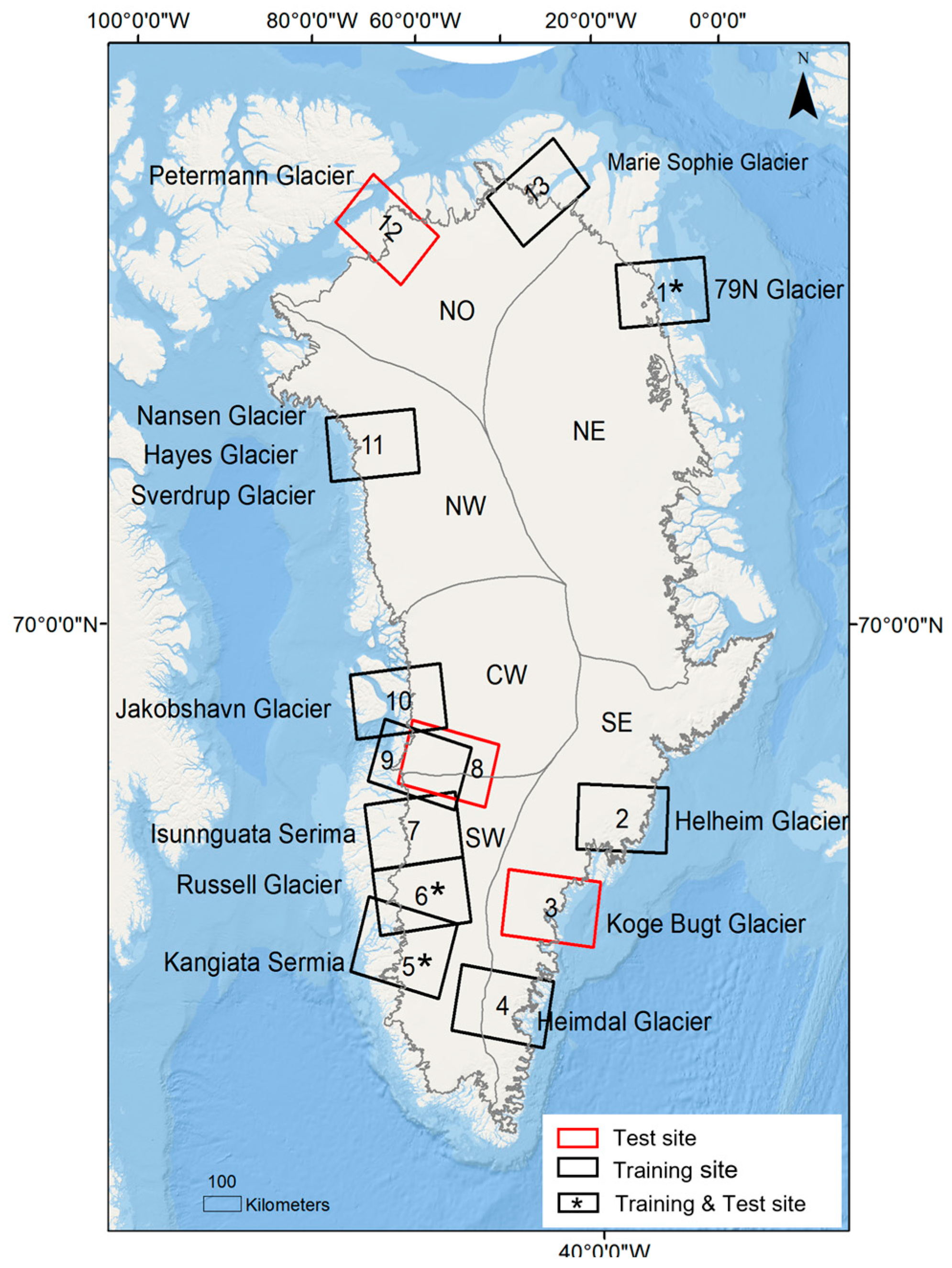
2.1. Study Sites
2.2. Datasets
2.2.1. Sentinel-1 SAR Data
2.2.2. Auxiliary Data
- Sentinel-2 data
- 2.
- DEM data
- 3.
- Coastline data
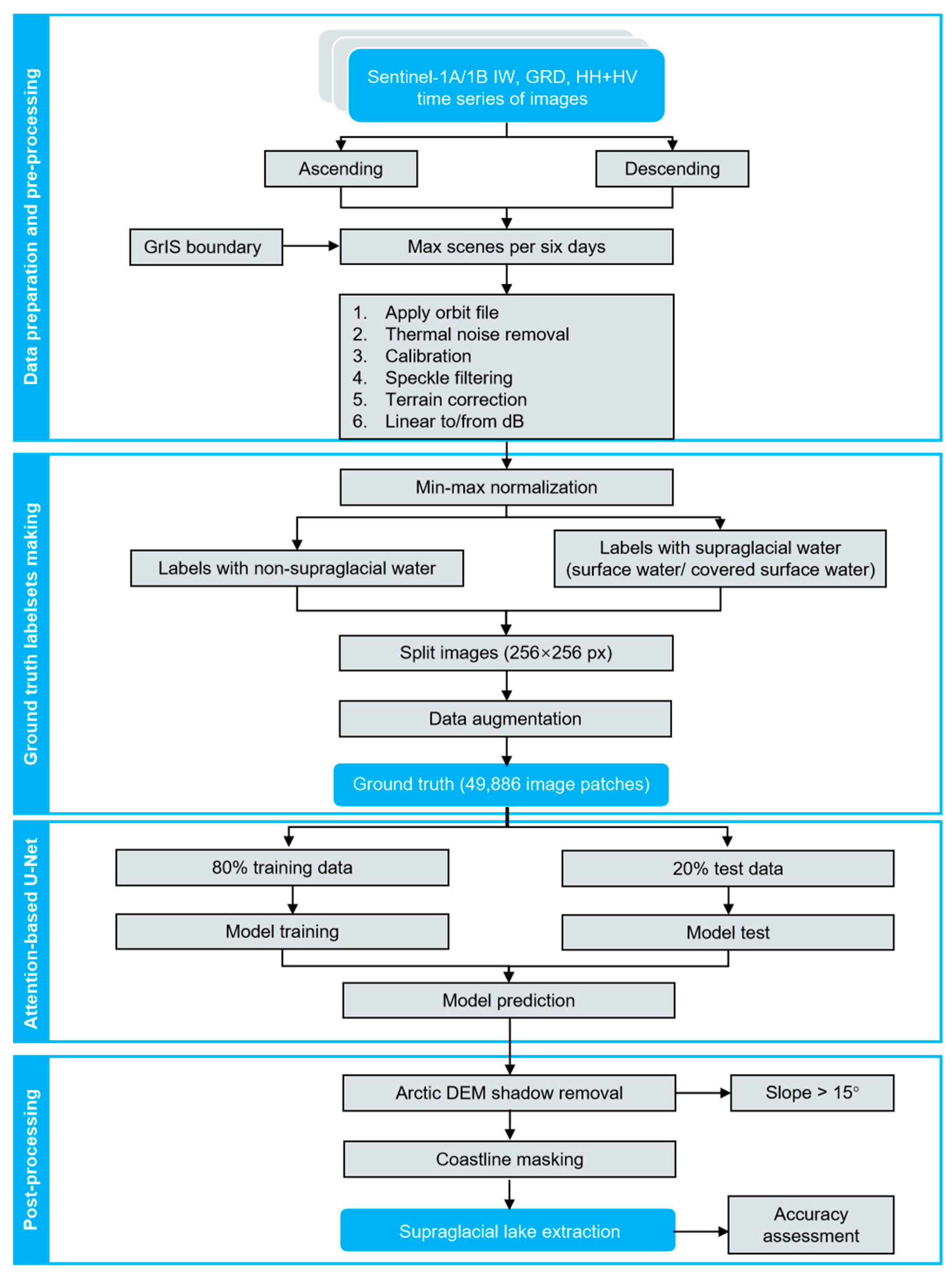
2.3. Method
2.3.1. Data Preprocessing
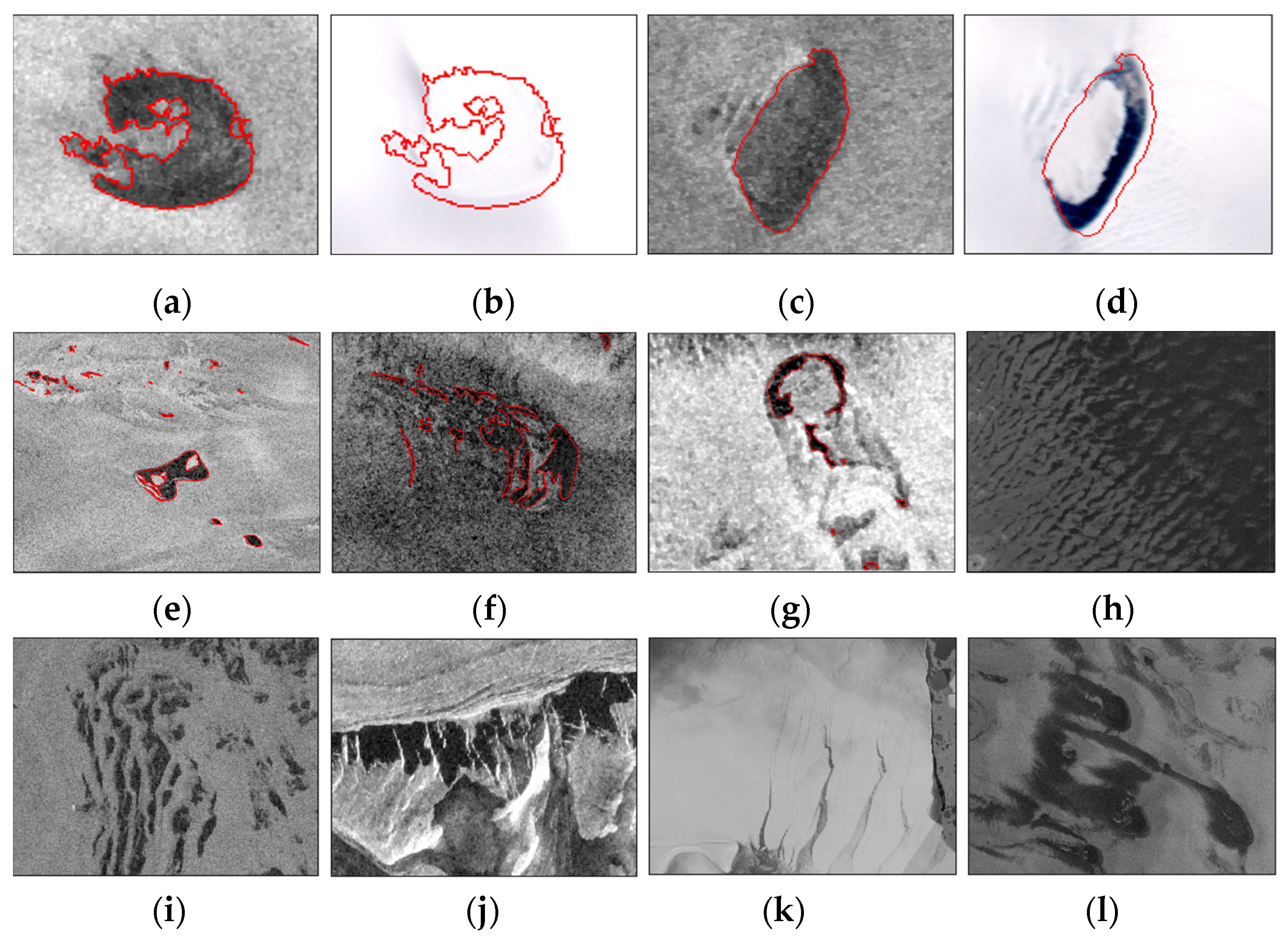
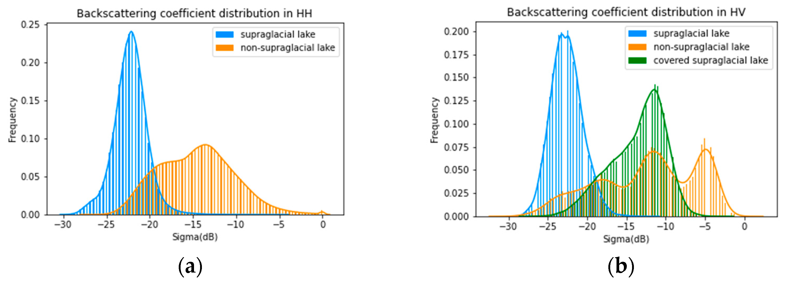
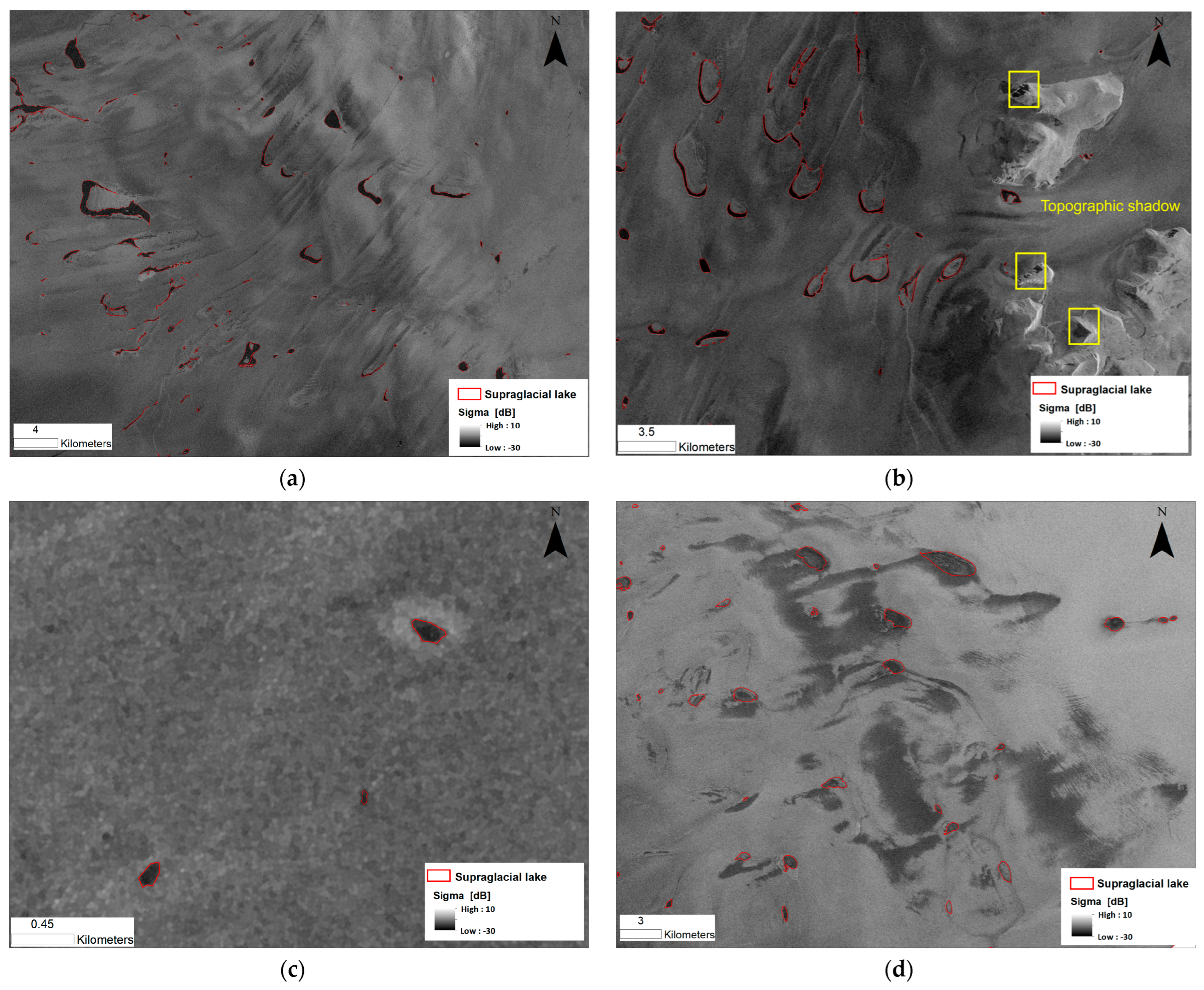
2.3.2. Supraglacial Lake in SAR
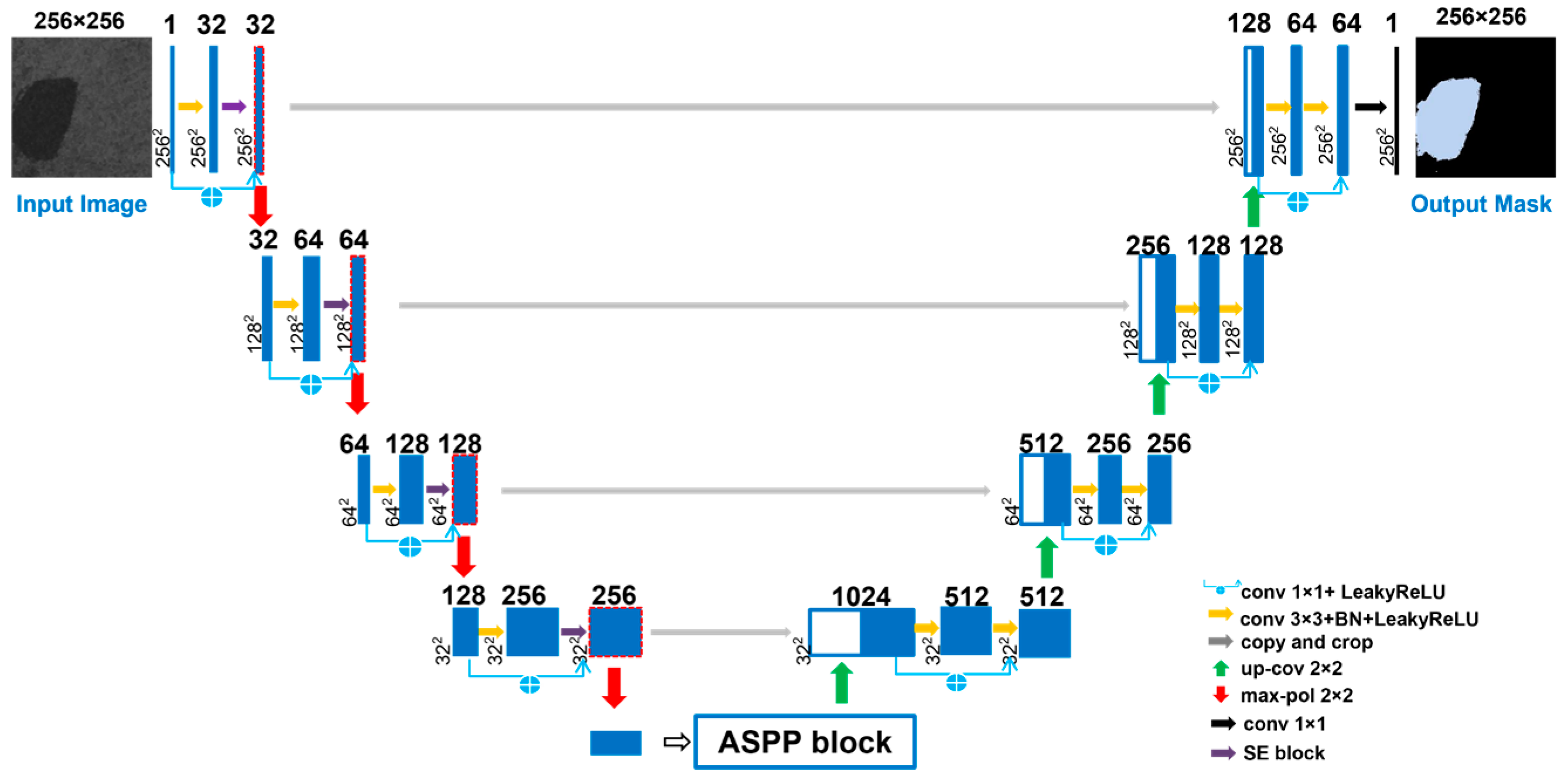
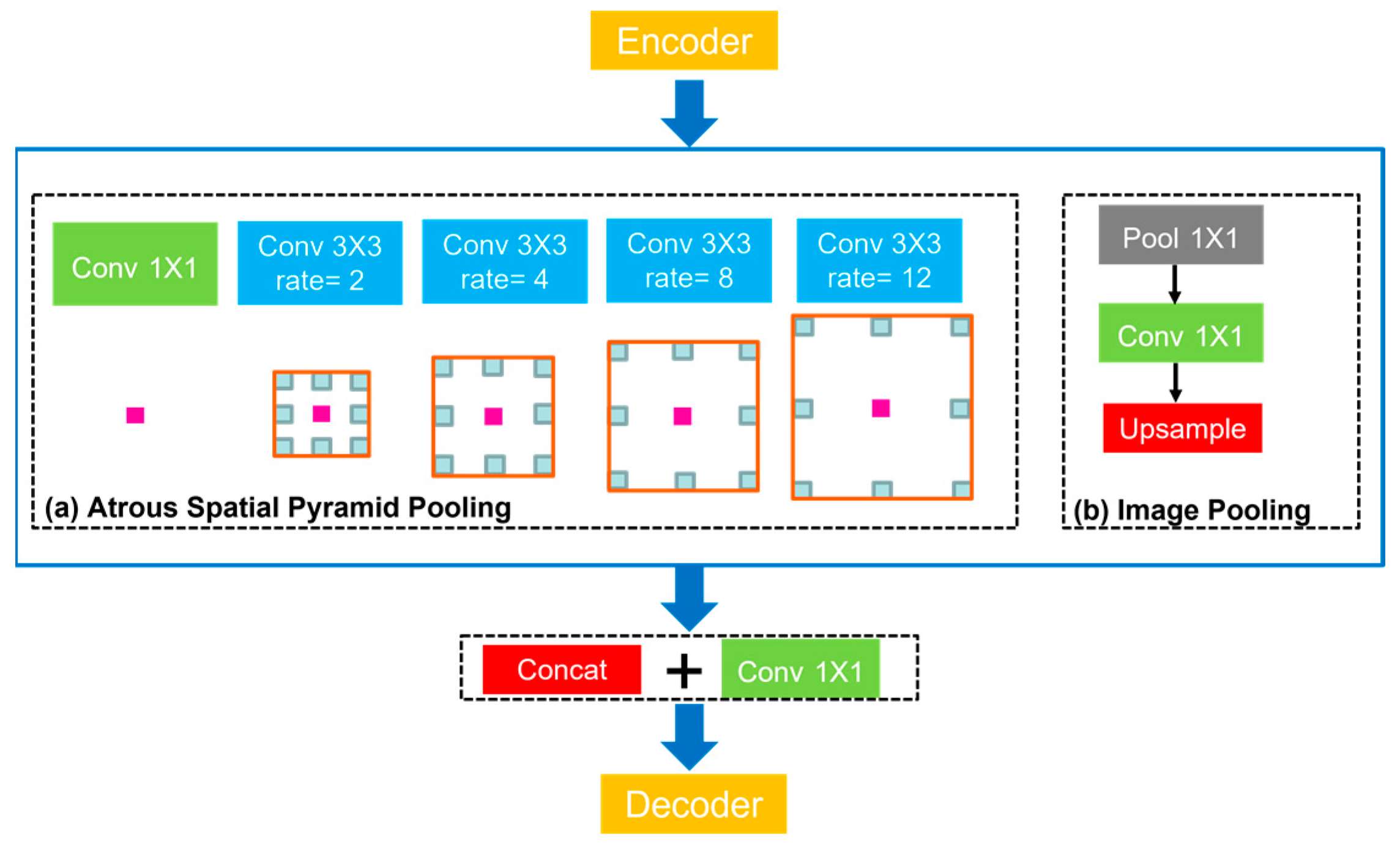
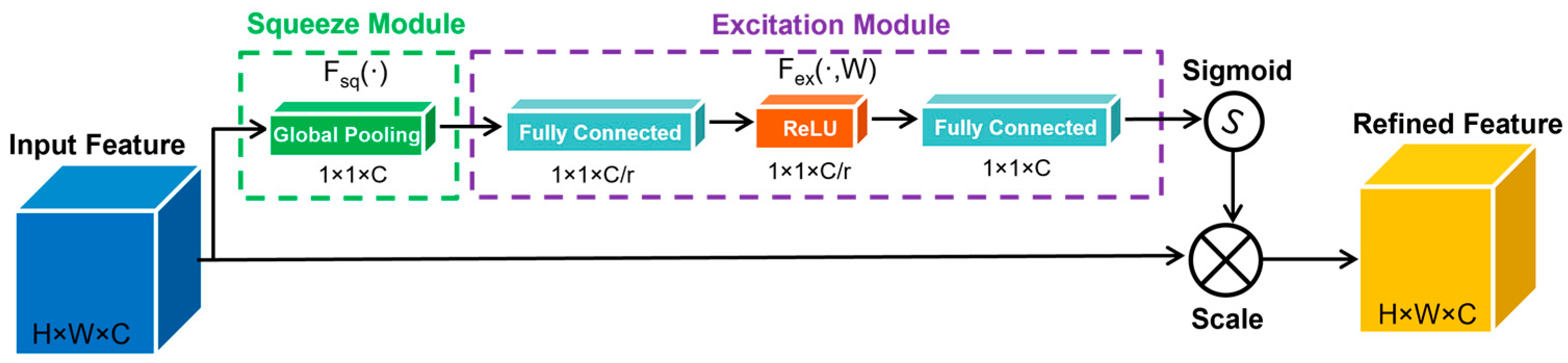
2.3.3. Attention-Based U-Net Architecture
2.3.4. Loss Function
2.3.5. Post-Processing
2.3.6. Accuracy Assessment
3. Results
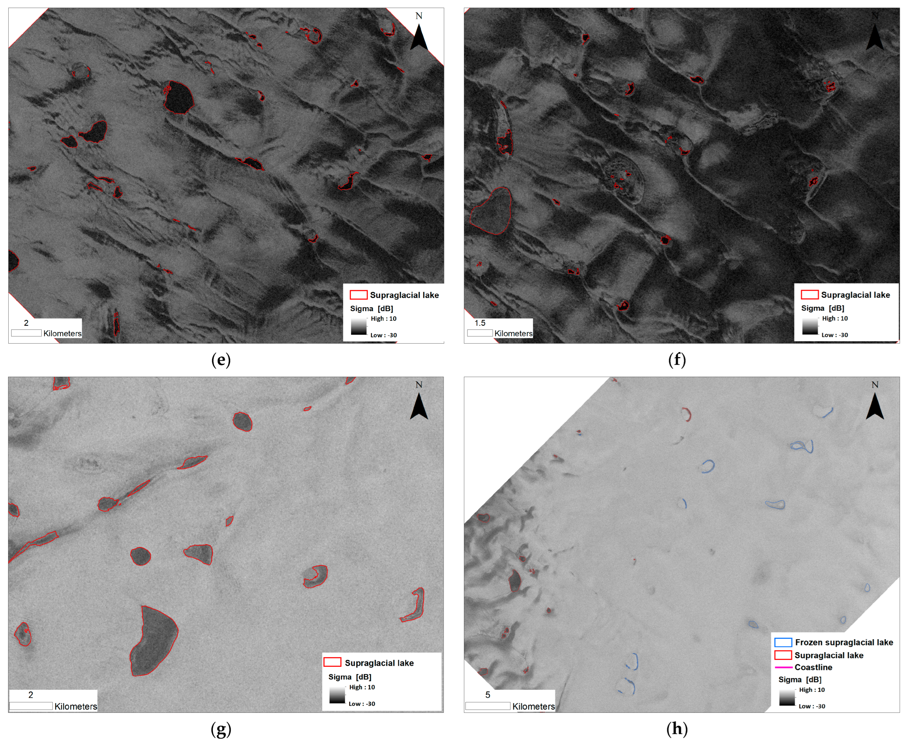
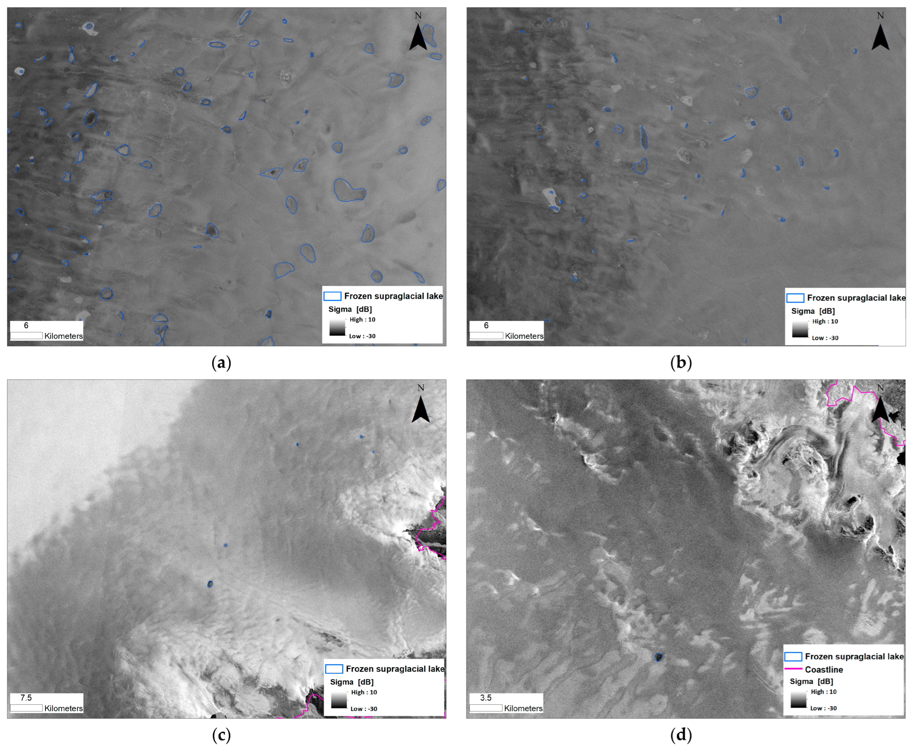
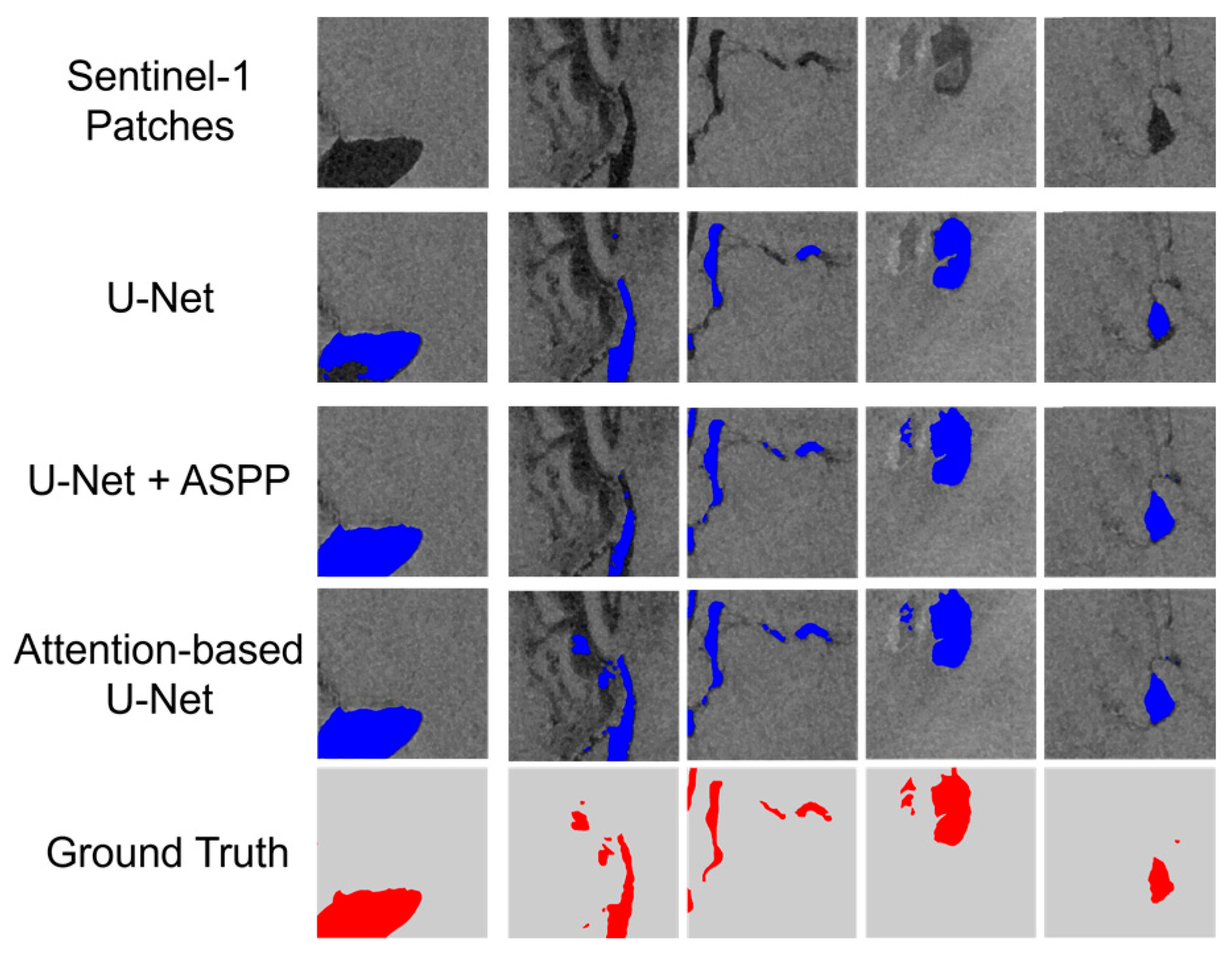
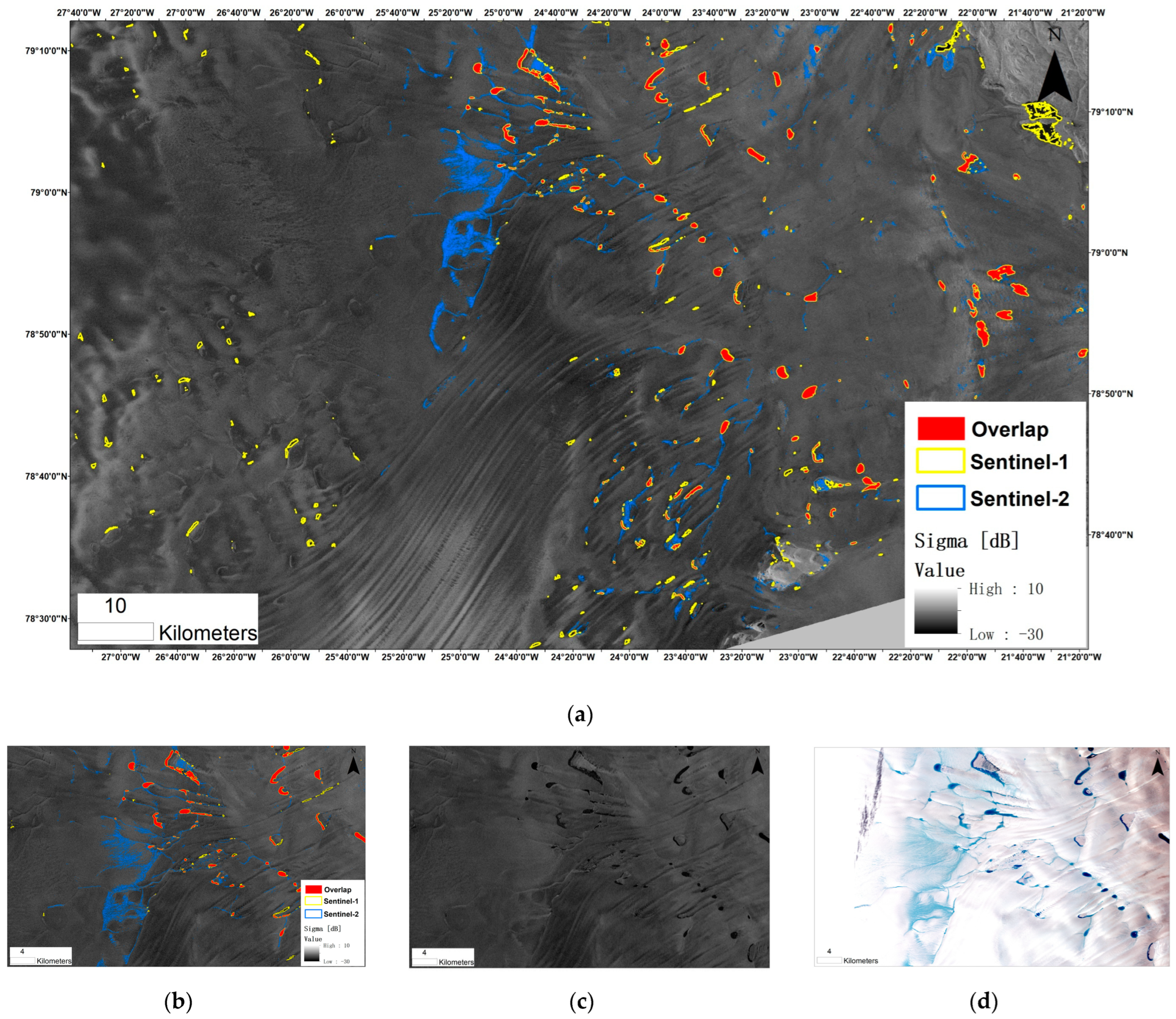
3.1. Automatic Extraction of Supraglacial Lakes
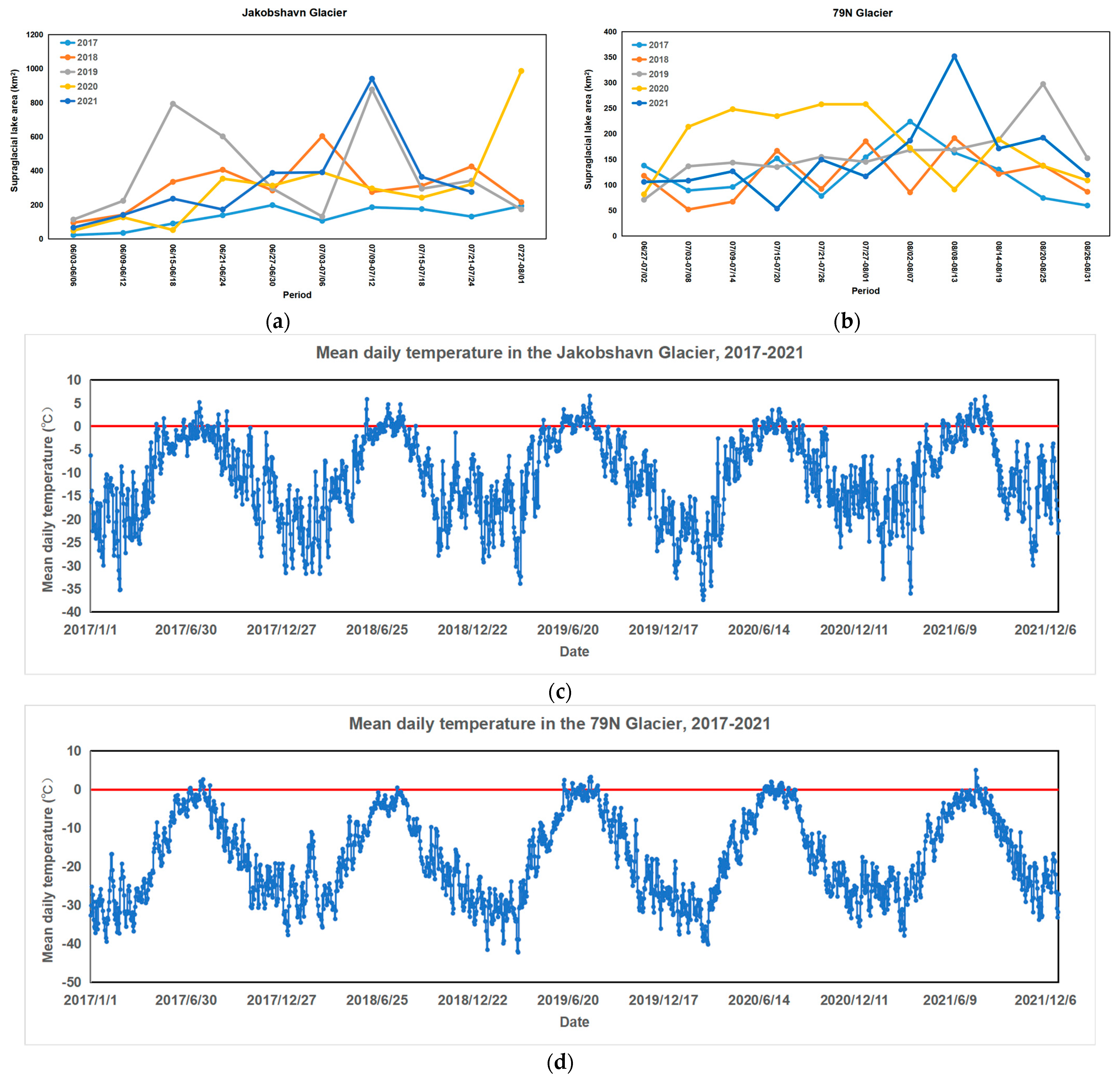
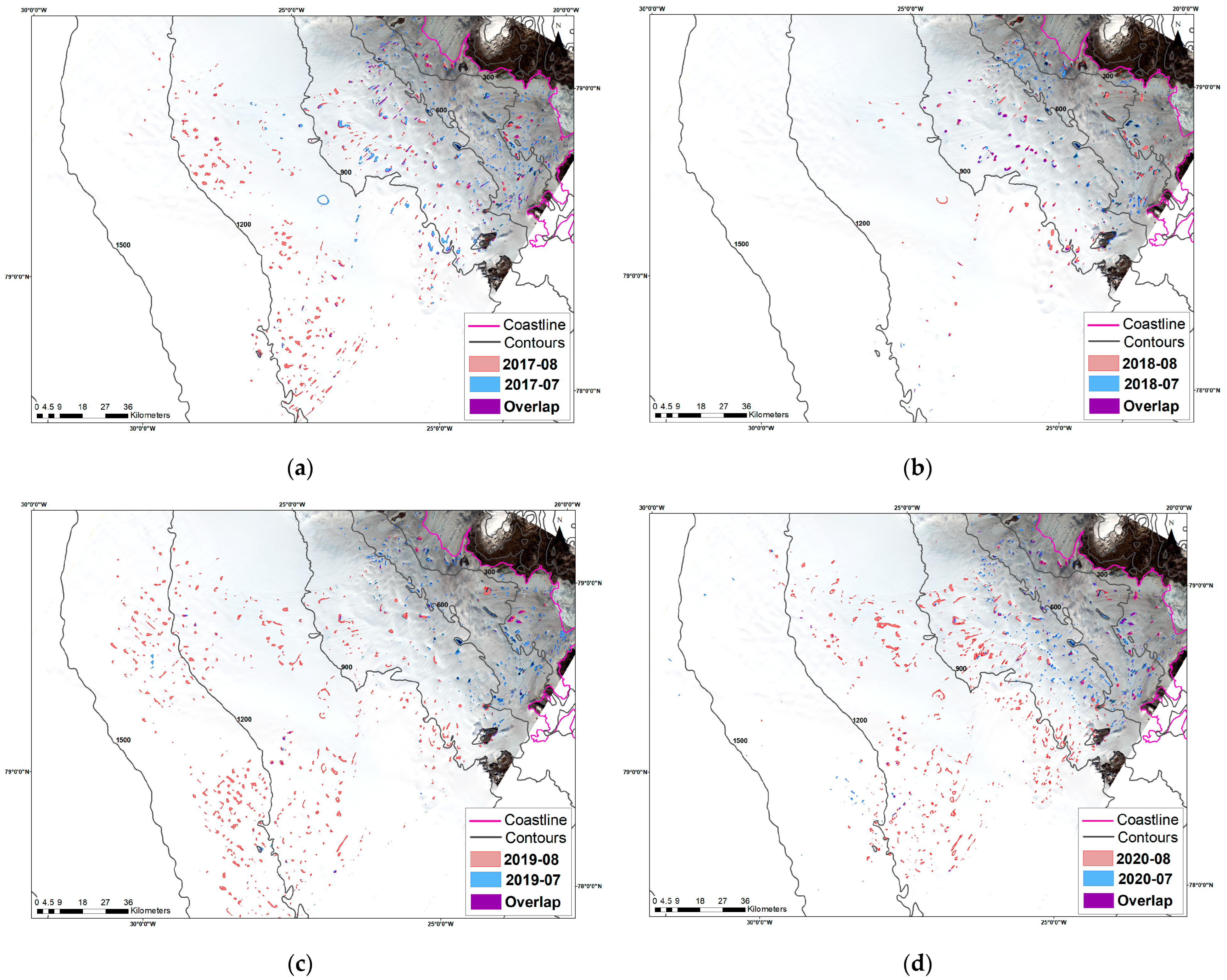
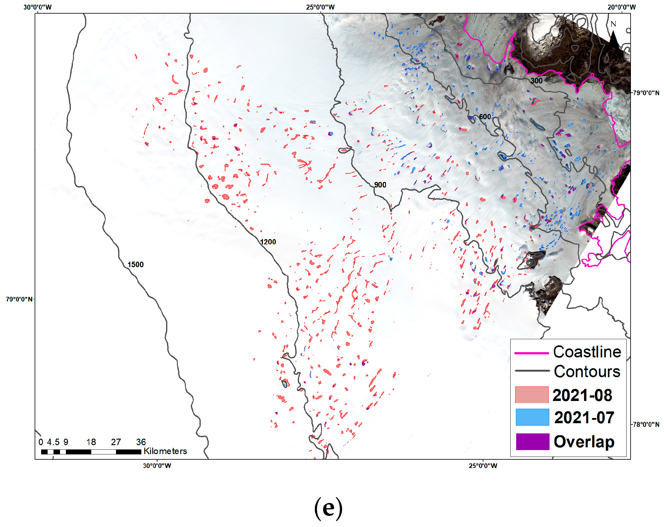
3.2. Spatiotemporal Change Analysis of Supraglacial Lakes
4. Discussion
4.1. Extraction of Supraglacial Lakes
4.2. Spatiotemporal Change Analysis
5. Conclusions
Author Contributions
Funding
Data Availability Statement
Acknowledgments
Conflicts of Interest
References
- Morlighem, M.; Williams, C.N.; Rignot, E.; An, L.; Arndt, J.E.; Bamber, J.L.; Catania, G.; Chauché, N.; Dowdeswell, J.A.; Dorschel, B.; et al. BedMachine v3: Complete Bed Topography and Ocean Bathymetry Mapping of Greenland from Multibeam Echo Sounding Combined with Mass Conservation. Geophys. Res. Lett. 2017, 44, 11051–11061. [Google Scholar] [CrossRef] [PubMed] [Green Version]
- Legg, S. IPCC, 2021: Climate Change 2021-the Physical Science basis. Interaction 2021, 49, 44–45. [Google Scholar] [CrossRef]
- Mouginot, J.; Rignot, E.; Bjørk, A.A.; Broeke, M.V.D.; Millan, R.; Morlighem, M.; Noël, B.; Scheuchl, B.; Wood, M. Forty-six years of Greenland Ice Sheet mass balance from 1972 to 2018. Proc. Natl. Acad. Sci. USA 2019, 116, 9239–9244. [Google Scholar] [CrossRef] [PubMed] [Green Version]
- King, M.D.; Howat, I.M.; Jeong, S.; Noh, M.J.; Wouters, B.; Noël, B.; Broeke, M.R.V.D. Seasonal to decadal variability in ice discharge from the Greenland Ice Sheet. Cryosphere 2018, 12, 3813–3825. [Google Scholar] [CrossRef] [Green Version]
- Yang, K.; Smith, L.C.; Fettweis, X.; Gleason, C.J.; Lu, Y.; Li, M. Surface meltwater runoff on the Greenland ice sheet estimated from remotely sensed supraglacial lake infilling rate. Remote Sens. Environ. 2019, 234, 111459. [Google Scholar] [CrossRef] [Green Version]
- Stevens, L.A.; Behn, M.D.; McGuire, J.J.; Das, S.B.; Joughin, I.; Herring, T.; Shean, D.E.; King, M.A. Greenland supraglacial lake drainages triggered by hydrologically induced basal slip. Nature 2015, 522, 73–76. [Google Scholar] [CrossRef]
- Lai, C.-Y.; Stevens, L.A.; Chase, D.L.; Creyts, T.T.; Behn, M.D.; Das, S.B.; Stone, H.A. Hydraulic transmissivity inferred from ice-sheet relaxation following Greenland supraglacial lake drainages. Nat. Commun. 2021, 12, 3955. [Google Scholar] [CrossRef]
- Arthur, J.F.; Stokes, C.; Jamieson, S.S.; Carr, J.R.; Leeson, A.A. Recent understanding of Antarctic supraglacial lakes using satellite remote sensing. Prog. Phys. Geogr. Earth Environ. 2020, 44, 837–869. [Google Scholar] [CrossRef]
- Doyle, S.H.; Hubbard, A.L.; Dow, C.F.; Jones, G.A.; Fitzpatrick, A.; Gusmeroli, A.; Kulessa, B.; Lindback, K.; Pettersson, R.; Box, J.E. Ice tectonic deformation during the rapid in situ drainage of a supraglacial lake on the Greenland Ice Sheet. Cryosphere 2013, 7, 129–140. [Google Scholar] [CrossRef] [Green Version]
- Chudley, T.R.; Christoffersen, P.; Doyle, S.H.; Bougamont, M.; Schoonman, C.M.; Hubbard, B.; James, M.R. Supraglacial lake drainage at a fast-flowing Greenlandic outlet glacier. Proc. Natl. Acad. Sci. USA 2019, 116, 25468–25477. [Google Scholar] [CrossRef]
- Langley, E.S.; Leeson, A.A.; Stokes, C.R.; Jamieson, S.S.R. Seasonal evolution of supraglacial lakes on an East Antarctic outlet glacier. Geophys. Res. Lett. 2016, 43, 8563–8571. [Google Scholar] [CrossRef]
- Sundal, A.; Shepherd, A.; Nienow, P.; Hanna, E.; Palmer, S.; Huybrechts, P. Evolution of supra-glacial lakes across the Greenland Ice Sheet. Remote Sens. Environ. 2009, 113, 2164–2171. [Google Scholar] [CrossRef]
- Everett, A.; Murray, T.; Selmes, N.; Rutt, I.C.; Luckman, A.; James, T.D.; Clason, C.; O’Leary, M.; Karunarathna, H.; Moloney, V.; et al. Annual down-glacier drainage of lakes and water-filled crevasses at Helheim Glacier, southeast Greenland. J. Geophys. Res. Earth Surf. 2016, 121, 1819–1833. [Google Scholar] [CrossRef] [Green Version]
- Williamson, A.G.; Arnold, N.S.; Banwell, A.; Willis, I.C. A Fully Automated Supraglacial lake area and volume Tracking (“FAST”) algorithm: Development and application using MODIS imagery of West Greenland. Remote Sens. Environ. 2017, 196, 113–133. [Google Scholar] [CrossRef]
- Stokes, C.R.; Sanderson, J.E.; Miles, B.; Jamieson, S.S.R.; Leeson, A. Widespread distribution of supraglacial lakes around the margin of the East Antarctic Ice Sheet. Sci. Rep. 2019, 9, 13823. [Google Scholar] [CrossRef] [Green Version]
- Moussavi, M.; Pope, A.; Halberstadt, A.; Trusel, L.; Cioffi, L.; Abdalati, W. Antarctic Supraglacial Lake Detection Using Landsat 8 and Sentinel-2 Imagery: Towards Continental Generation of Lake Volumes. Remote Sens. 2020, 12, 134. [Google Scholar] [CrossRef] [Green Version]
- Hochreuther, P.; Neckel, N.; Reimann, N.; Humbert, A.; Braun, M. Fully Automated Detection of Supraglacial Lake Area for Northeast Greenland Using Sentinel-2 Time-Series. Remote Sens. 2021, 13, 205. [Google Scholar] [CrossRef]
- Dirscherl, M.; Dietz, A.; Kneisel, C.; Kuenzer, C. A Novel Method for Automated Supraglacial Lake Mapping in Antarctica Using Sentinel-1 SAR Imagery and Deep Learning. Remote Sens. 2021, 13, 197. [Google Scholar] [CrossRef]
- Dirscherl, M.C.; Dietz, A.J.; Kuenzer, C. Seasonal evolution of Antarctic supraglacial lakes in 2015–2021 and links to environmental controls. Cryosphere 2021, 15, 5205–5226. [Google Scholar] [CrossRef]
- Chen, F. Comparing Methods for Segmenting Supra-Glacial Lakes and Surface Features in the Mount Everest Region of the Himalayas Using Chinese GaoFen-3 SAR Images. Remote Sens. 2021, 13, 2429. [Google Scholar] [CrossRef]
- Jiang, D.; Li, X.; Xiang, Q.; Ma, M.; Hong, W.; Wu, Y. Automated extraction for Supraglacial lake in Greenland using Sentinel-1 SAR Imagery. In Proceedings of the 2021 IEEE International Geoscience and Remote Sensing Symposium IGARSS, Brussels, Belgium, 11–16 July 2021; IEEE: Piscataway, NJ, USA, 2021; pp. 5501–5504. [Google Scholar] [CrossRef]
- Miles, K.E.; Willis, I.C.; Benedek, C.L.; Williamson, A.G.; Tedesco, M. Toward Monitoring Surface and Subsurface Lakes on the Greenland Ice Sheet Using Sentinel-1 SAR and Landsat-8 OLI Imagery. Front. Earth Sci. 2017, 5, 58. [Google Scholar] [CrossRef] [Green Version]
- Schröder, L.; Neckel, N.; Zindler, R.; Humbert, A. Perennial Supraglacial Lakes in Northeast Greenland Observed by Polarimetric SAR. Remote Sens. 2020, 12, 2798. [Google Scholar] [CrossRef]
- Benedek, C.L.; Willis, I.C. Winter drainage of surface lakes on the Greenland Ice Sheet from Sentinel-1 SAR imagery. Cryosphere 2021, 15, 1587–1606. [Google Scholar] [CrossRef]
- Koenig, L.S.; Lampkin, D.J.; Montgomery, L.N.; Hamilton, S.L.; Turrin, J.B.; Joseph, C.A.; Moutsafa, S.E.; Panzer, B.; Casey, K.A.; Paden, J.D.; et al. Wintertime storage of water in buried supraglacial lakes across the Greenland Ice Sheet. Cryosphere 2015, 9, 1333–1342. [Google Scholar] [CrossRef] [Green Version]
- Rignot, E.; Echelmeyer, K.; Krabill, W. Penetration depth of interferometric synthetic-aperture radar signals in snow and ice. Geophys. Res. Lett. 2001, 28, 3501–3504. [Google Scholar] [CrossRef] [Green Version]
- Seroussi, H.; Morlighem, M.; Rignot, E.; Larour, E.; Aubry, D.; Ben Dhia, H.; Kristensen, S.S. Ice flux divergence anomalies on 79°N Glacier, Greenland. Geophys. Res. Lett. 2011, 38, L09501. [Google Scholar] [CrossRef] [Green Version]
- Turton, J.V.; Hochreuther, P.; Reimann, N.; Blau, M.T. The distribution and evolution of supraglacial lakes on 79°N Glacier (north-eastern Greenland) and interannual climatic controls. Cryosphere 2021, 15, 3877–3896. [Google Scholar] [CrossRef]
- Lemos, A.; Shepherd, A.; McMillan, M.; Hogg, A.E. Seasonal Variations in the Flow of Land-Terminating Glaciers in Central-West Greenland Using Sentinel-1 Imagery. Remote Sens. 2018, 10, 1878. [Google Scholar] [CrossRef] [Green Version]
- Rowley, N.A.; Fegyveresi, J.M. Generating a supraglacial melt-lake inventory near Jakobshavn, West Greenland, using a new semi-automated lake-mapping technique. Polar Geogr. 2019, 42, 89–108. [Google Scholar] [CrossRef]
- Macdonald, G.J.; Banwell, A.F.; MacAyeal, D.R. Seasonal evolution of supraglacial lakes on a floating ice tongue, Petermann Glacier, Greenland. Ann. Glaciol. 2018, 59, 56–65. [Google Scholar] [CrossRef] [Green Version]
- Geudtner, D.; Torres, R.; Snoeij, P.; Davidson, M.; Rommen, B. Sentinel-1 System capabilities and applications. In Proceedings of the 2014 IEEE International Geoscience and Remote Sensing Symposium (IGARSS), Quebec City, QC, Canada, 13–18 July 2014; IEEE: Piscataway, NJ, USA, 2014; pp. 1457–1460. [Google Scholar] [CrossRef]
- Center, P.G.; Porter, C.; Morin, P.; Howat, I.; Noh, M.; Bates, B.; Bojesen, M. ArcticDEM. In Harvard Dataverse; JSTOR: New York, NY, USA, 2018; Volume 1, p. 201. [Google Scholar] [CrossRef]
- He, K.; Zhang, X.; Ren, S.; Sun, J. Deep residual learning for image recognition. In Proceedings of the 2016 IEEE Conference on Computer Vision and Pattern Recognition (CVPR), Las Vegas, NV, USA, 27–30 June 2016; pp. 770–778. [Google Scholar] [CrossRef] [Green Version]
- Hu, J.; Shen, L.; Sun, G. Squeeze-and-Excitation Networks. In Proceedings of the IEEE Conference on Computer Vision and Pattern Recognition (CVPR), Salt Lake City, UT, USA, 18–23 June 2018; pp. 7132–7141. [Google Scholar]
- Wang, J.; Lv, P.; Wang, H.; Shi, C. SAR-U-Net: Squeeze-and-excitation block and atrous spatial pyramid pooling based residual U-Net for automatic liver segmentation in Computed Tomography. Comput. Methods Programs Biomed. 2021, 208, 106268. [Google Scholar] [CrossRef] [PubMed]
- Hu, J.; Huang, H.; Chi, Z.; Cheng, X.; Wei, Z.; Chen, P.; Xu, X.; Qi, S.; Xu, Y.; Zheng, Y. Distribution and Evolution of Supraglacial Lakes in Greenland during the 2016–2018 Melt Seasons. Remote Sens. 2021, 14, 55. [Google Scholar] [CrossRef]
- Box, J.E.; Wehrlé, A.; van As, D.; Fausto, R.S.; Kjeldsen, K.K.; Dachauer, A.; Ahlstrøm, A.P.; Picard, G. Greenland Ice Sheet Rainfall, Heat and Albedo Feedback Impacts from the Mid-August 2021 Atmospheric River. Geophys. Res. Lett. 2022, 49, e2021GL097356. [Google Scholar] [CrossRef]
- How, P.; Messerli, A.; Mätzler, E.; Santoro, M.; Wiesmann, A.; Caduff, R.; Langley, K.; Bojesen, M.H.; Paul, F.; Kääb, A.; et al. Greenland-wide inventory of ice marginal lakes using a multi-method approach. Sci. Rep. 2021, 11, 4481. [Google Scholar] [CrossRef] [PubMed]
- Lampkin, D.J.; Koenig, L.; Joseph, C.; Box, J.E. Investigating Controls on the Formation and Distribution of Wintertime Storage of Water in Supraglacial Lakes. Front. Earth Sci. 2020, 8, 370. [Google Scholar] [CrossRef]
- Law, R.; Arnold, N.; Benedek, C.; Tedesco, M.; Banwell, A.; Willis, I. Over-winter persistence of supraglacial lakes on the Greenland Ice Sheet: Results and insights from a new model. J. Glaciol. 2020, 66, 362–372. [Google Scholar] [CrossRef]
- Selmes, N.; Murray, T.; James, T. Characterizing supraglacial lake drainage and freezing on the Greenland Ice Sheet. Cryosphere Discuss. 2013, 7, 475–505. [Google Scholar] [CrossRef]


| ID | Acquisition Date | Path | Study Region | Flight Direction | Type |
|---|---|---|---|---|---|
| S1-01 | 10 August 2020 | 207 | NE | Descending | Training/Test |
| S1-02 | 27 August 2021 | 141 | SE | Descending | Training |
| S1-03 | 18 October 2021 | 112 | SE | Descending | Test |
| S1-04 | 29 September 2021 | 10 | SE | Descending | Training |
| S1-05 | 7 July 2017 | 54 | SW | Descending | Training/Test |
| S1-06 | 12 February 2021 | 90 | SW | Ascending | Training/Test |
| S1-07 | 17 July 2020 | 90 | SW | Ascending | Training |
| S1-08 | 21 February 2019 | 54 | CW | Descending | Test |
| S1-09 | 7 August 2020 | 127 | CW | Descending | Training |
| S1-10 | 28 August 2020 | 90 | CW | Ascending | Training |
| S1-11 | 11 February 2019 | 90 | NW | Descending | Training |
| S1-12 | 2 January 2019 | 26 | NO | Descending | Test |
| S1-13 | 27 September 2021 | 74 | NO | Ascending | Training |
| Method | A | R | P | F1 |
|---|---|---|---|---|
| U-Net | 0.979 | 0.845 | 0.849 | 0.839 |
| U-Net + ASPP | 0.993 | 0.979 | 0.954 | 0.966 |
| Attention-based U-Net | 0.994 | 0.988 | 0.956 | 0.971 |
Publisher’s Note: MDPI stays neutral with regard to jurisdictional claims in published maps and institutional affiliations. |
© 2022 by the authors. Licensee MDPI, Basel, Switzerland. This article is an open access article distributed under the terms and conditions of the Creative Commons Attribution (CC BY) license (https://creativecommons.org/licenses/by/4.0/).
Share and Cite
Jiang, D.; Li, X.; Zhang, K.; Marinsek, S.; Hong, W.; Wu, Y. Automatic Supraglacial Lake Extraction in Greenland Using Sentinel-1 SAR Images and Attention-Based U-Net. Remote Sens. 2022, 14, 4998. https://doi.org/10.3390/rs14194998
Jiang D, Li X, Zhang K, Marinsek S, Hong W, Wu Y. Automatic Supraglacial Lake Extraction in Greenland Using Sentinel-1 SAR Images and Attention-Based U-Net. Remote Sensing. 2022; 14(19):4998. https://doi.org/10.3390/rs14194998
Chicago/Turabian StyleJiang, Di, Xinwu Li, Ke Zhang, Sebastián Marinsek, Wen Hong, and Yirong Wu. 2022. "Automatic Supraglacial Lake Extraction in Greenland Using Sentinel-1 SAR Images and Attention-Based U-Net" Remote Sensing 14, no. 19: 4998. https://doi.org/10.3390/rs14194998